Covariance matrix entanglement criterion for an arbitrary set of operators

Abstract

We generalize entanglement detection with covariance matrices for an arbitrary set of observables. A generalized uncertainty relation is constructed using the covariance and commutation matrices, then a criterion is established by performing a partial transposition on the operators. The method is highly efficient and versatile in the sense that the set of measurement operators can be freely chosen, do not need to be complete, and there is no constraint on the commutation relations. The method is particularly suited for systems with higher dimensionality since the computations do not scale with the dimension of the Hilbert space — rather they scale with the number of chosen observables which can always be kept small. We illustrate the approach by examining the entanglement between two spin ensembles, and show that it detects entanglement in a basis independent way.

I Introduction

Entanglement is a key resource for many quantum information technologies and detecting its presence is a fundamental experimental task. Numerous methods for the detection and quantification of entanglement have been studied in great depth for bipartite and multipartite systems horod ; guhne2009entanglement ; eisert2007quantitative ; vedral2008quantifying ; plenio2005introduction . For systems with small Hilbert space dimension, one standard approach is to reconstruct the density matrix and perform a positive partial transpose (PPT) test to check for separability peres ; Horodecki19961 ; HORODECKI1997333 ; PhysRevLett.95.090503 ; vidal2002computable . However, this requires full tomography of the density matrix, which for systems with large Hilbert space may be impractical or even impossible to measure. In this case what is most desirable (e.g. from an experimental point of view) are simple criteria that can be evaluated based on a small number of observables. In this sense, criteria such as those given by Duan and co-workers Duan , Hillery-Zubairy hillery , entanglement witness horedecki1996separability ; PhysRevA.62.052310 ; szangolies2015detecting ; singh2016entanglement , mutually unbiased bases PhysRevA.86.022311 , and others toth2006detection ; PhysRevA.92.022339 ; wu2005entanglement ; PhysRevA.95.052305 ; de2011multipartite ; altepeter2005experimental are quite valuable as they can detect entanglement without full tomography of the density matrix.

For continuous variables, a powerful method to detect entanglement has been developed based on the covariance matrix simon ; Duan ; braunstein ; adesso2007entanglement ; wang2007quantum ; werner . In the approach, one has observables corresponding to the quadrature pairs in two subsystems (labeled by $A$ and $B$) $\xi=(x_{A},p_{A},x_{B},p_{B})$ where $[x,p]=i$. Defining the covariance matrix, one may determine a sufficient condition for entanglement simon ; Duan . Despite its great success for optical systems, for other systems, it has been more challenging to define analogous quantities. Generalization to nonlinear systems guhne2007nonlinear and necessary and sufficient inseparability conditions for symmetric qubits have been performed (usha, ; gittsov, ). In particular, a more general framework for finite systems and a generalized set of measurement operators was performed by Gühne, Eisert, and co-workers, with several entanglement criteria defined accordingly guhne2007 ; PhysRevA.81.032333 . While this allows for a more generalized application of the approach, the approach requires a complete set of observables to construct the covariance matrix li2008separability . For a large but finite systems, such as two atomic spin ensembles or Bose-Einstein condensates, this makes it difficult to apply in practice, since measurements scaling as the square of the dimension of the Hilbert space are needed polzik ; andrew ; eisert . What would be more desirable is to have a covariance matrix approach that is based on a finite set of freely choosable measurements, and applicable to any system, both finite and infinite.

In this paper, we generalize the covariance matrix approach to an arbitrary set of measurement operators, that satisfy arbitrary commutation relations. The situation that is most relevant to our formalism is as follows. Consider that a set of correlations $\langle\xi_{j}\xi_{k}\rangle$ and expectation values $\langle\xi_{j}\rangle$ has been measured (e.g. from an experiment), where $\xi_{j}$ are an arbitrary set of $N$ known observables. The task is then to take this data and determine whether entanglement is present between two subsystems, $A$ and $B$. In the situation we consider, we assume that an arbitrary entanglement witness operator is not in general constructable using the $\xi_{j}$ operators, hence the question is how best to extract the information regarding entanglement from the given correlations. Our approach is to construct a covariance matrix and a commutation matrix, which together can be used to determine the presence of entanglement. Since the number of observables $N$ is typically quite small, this is a highly efficient procedure for detecting entanglement since it only requires diagonalization of a $N\times N$ matrix. This is in contrast to alternative entanglement detection methods which can require computations scaling with the Hilbert space dimension $D\gg N$, which can potentially be large.

II Covariance and commutator matrix

We start with defining a set of $N$ observables (Hermitian operators) $\xi_{n}$ on the composite system $A$ and $B$, with $n\in[1,N]$. The dimension of the Hilbert space of the composite system is $D$. All these operators can be collected in a vector

$$\xi=({\cal\xi}_{1},{\cal\xi}_{2}\dots,{\cal\xi}_{N})$$ (1)

where these operators are general so that they could come from either subsystem $A$, $B$, or both. The $N\times N$ covariance matrix is defined in the standard way

$$V_{jk}\equiv\frac{1}{2}\langle\{\xi_{j},\xi_{k}\}\rangle-\langle\xi_{j}\rangle\langle\xi_{k}\rangle,$$ (2)

which is a real symmetric matrix and $\{X,Y\}=XY+YX$ is the anticommutator. The $N\times N$ commutation matrix for $j,k\in[1,N]$ is defined as

$$\Omega_{jk}\equiv-i\langle[\xi_{j},\xi_{k}]\rangle,$$ (3)

which is a real antisymmetric matrix .

The matrix inequation

$$V+\frac{i}{2}\Omega\geq 0$$ (4)

succinctly summarizes the uncertainty relation between the operators $\xi_{j}$ simon ; simonearlypaper . For the purposes of the relation (4) there is no role played by the subsystems $A,B$ and hence we may consider $\xi$ to contain an arbitrary set of $N$ operators. The meaning of (4) is in terms of the semi-positive nature of the matrix, i.e. that it has no negative eigenvalues. In Ref. simonearlypaper this was shown for the case of quadratures. We show here that in fact this generalizes to arbitrary number and type of operators. To see the power of the relation (4) consider the generalized uncertainty relation for an arbitrary number of operators. The Schrodinger uncertainty relation gives the relationship bounding the product of the variances between two operators $\xi_{1},\xi_{2}$

$${\cal I}_{12}\equiv \sigma^{2}_{\xi_{1}}\sigma^{2}_{\xi_{2}}-\left|\frac{\langle\{\xi_{1},\xi_{2}\}\rangle}{2}-\langle\xi_{1}\rangle\langle\xi_{2}\rangle\right|^{2}-\left|\frac{\langle[\xi_{1},\xi_{2}]\rangle}{2i}\right|^{2}\geq 0,$$

where $\sigma^{2}_{\xi}\equiv\langle\xi^{2}\rangle-\langle\xi\rangle^{2}$. Following the same procedure , one can straightforwardly derive the Schrodinger uncertainty relations for $N$ operators $\xi_{1},\dots,\xi_{N}$. For example, for $N=1$ one obtains ${\cal I}_{1}\equiv\sigma^{2}_{\xi_{1}}\geq 0$ and for $N=3$ we obtain

$${\cal I}_{123}\equiv \sigma^{2}_{\xi_{1}}\sigma^{2}_{\xi_{2}}\sigma^{2}_{\xi_{3}}-\langle{f_{1}}|f_{1}\rangle|\langle{f_{2}}|f_{3}\rangle|^{2}-\langle{f_{2}}|f_{2}\rangle|\langle{f_{3}}|f_{1}\rangle|^{2}$$

$$-\langle{f_{1}}|f_{2}\rangle\langle{f_{2}}|f_{3}\rangle\langle{f_{3}}|f_{1}\rangle-\langle{f_{2}}|f_{1}\rangle\langle{f_{3}}|f_{2}\rangle\langle{f_{1}}|f_{3}\rangle$$

$$-\langle{f_{3}}|f_{3}\rangle|\langle{f_{1}}|f_{2}\rangle|^{2}\geq 0$$ (5)

where $|f_{i}\rangle=(\xi_{i}-\langle\xi_{i}\rangle)|\Psi\rangle$.

The remarkable feature of (4) is that it contains information about all the Schrodinger uncertainty relations as described above. Taking for example the $N=3$ case, the first order invariant of (4) yields ${\cal I}_{1}+{\cal I}_{2}+{\cal I}_{3}\geq 0$, i.e. the sum of the variances of the operators is non-negative. The second order invariant (sum of principle minors) yields ${\cal I}_{12}+{\cal I}_{23}+{\cal I}_{13}\geq 0$, which is the sum of the standard Schrodinger uncertainty relation between all operator pairs. Finally, the third order invariant (i.e. the determinant) yields ${\cal I}_{123}\geq 0$, which is the three operator Schrodinger uncertainty relation. In the $N$-operator case, (4) summarizes the $1,2,\dots,N$-operator Schrodinger uncertainty relation via the matrix invariants in a highly succinct way.

While this connection to the uncertainty relation is beautiful, we should show explicitly that (4) is true for an arbitrary set of operators. In fact there is a simple way to show this in general without alluding to the uncertainty relation. Let us first write

$$V+\frac{i}{2}\Omega=\begin{pmatrix}\langle{f_{1}}|f_{1}\rangle&\ldots&\langle{f_{1}}|f_{N}\rangle\\ \vdots&\ddots&\vdots\\ \langle{f_{N}}|f_{1}\rangle&\ldots&\langle{f_{N}}|f_{N}\rangle\\ \end{pmatrix}.$$ (6)

This an overlap matrix, which is positive definite, immediately implying that $V+\frac{i}{2}\Omega>0$ for pure states overlap . Overlap matrices typically assume that none of the matrix elements are zero. Here we relax the condition and allow for the possibility that $\langle{f_{j}}|f_{k}\rangle=0$. This gives the additional possibility that the matrix can possess a zero eigenvalue, which shows the positive semi-definite nature of (4). For mixed states, we may use the fact that any density matrix can be diagonalized into a mixture of pure states $\rho=\sum_{l}p_{l}|\Psi_{l}\rangle\langle\Psi_{l}|$ and the concavity property of covariance matrices gitts to show that (4) is true for mixed states .

The matrix formalism is convenient as it automatically takes into account of symmetries that may be present in the operators $\xi_{j}$. The uncertainty relations are in terms of invariants of the matrix, hence they are guaranteed to be unchanged under these symmetry operations. For example, for the quantum optical case with operators $\xi=(x_{A},p_{A},x_{B},p_{B})$, symplectic transformations Sp(4) can be used to obtain another set of observables $\xi^{\prime}=(x_{A}^{\prime},p_{A}^{\prime},x_{B}^{\prime},p_{B}^{\prime})$ (simonearlypaper, ). The uncertainty relations are guaranteed to be unchanged under such a transformation. For the case of a spin ensemble that we examine later, we use observables $\xi=(S_{x},S_{y},S_{z})$, which can be rotated under a basis transformation under SO(3) to $\xi^{\prime}=(S_{x}^{\prime},S_{y}^{\prime},S_{z}^{\prime})$. Using a symmetrical set of operators, the particular basis that is used for the measurements becomes irrelevant.

III Entanglement detection

Now that we have established (4), we may see how this can be used in relation to detecting entanglement. We use the Peres-Horodecki criterion (peres, ; HORODECKI1997333, ; Horodecki19961, ) by performing a partial transpose (PT) operation on the density matrix operator. This PT operation on the density matrix operator will have a corresponding effect on the covariance matrix $V\rightarrow\text{PT}(V)$, which depends upon the particular operators that are used in $\xi$. The commutation matrix also is affected in the general case according to $\Omega\rightarrow\text{PT}(\Omega)$. Denoting the PT transposed density matrix as $\rho^{T_{B}}$, The PT transposition operation is defined as making the replacement $\rho\rightarrow\rho^{T_{B}}$ in all averages:

$$[\text{PT}(V)]_{jk} =\frac{1}{2}\text{Tr}(\rho^{T_{B}}\{\xi_{j},\xi_{k}\})-\text{Tr}(\rho^{T_{B}}\xi_{j})\text{Tr}(\rho^{T_{B}}\xi_{k})$$

$$[\text{PT}(\Omega)]_{jk} =-i\text{Tr}(\rho^{T_{B}}[\xi_{j},\xi_{k}]).$$ (7)

For a separable state, the PT operation should give a valid density matrix with positive eigenvalues. Thus the new covariance and commutation matrix necessarily satisfies

$$\text{PT}(V)+\frac{i}{2}\text{PT}(\Omega)\geq 0$$ (8)

if it is a separable bipartite state. Violation of (8) guarantees non-separability and thus entanglement in the bipartite system.

The usefulness of the above argument hinges upon the simple evaluation of (7). The partial transposed operator is not available by direct measurement, hence we require an equivalent expression in terms of the original density matrix. Due to the fact that $\text{Tr}(\rho^{T_{B}}X)=\text{Tr}(\rho X^{T_{B}})$, we have

$$[\text{PT}(V)+\frac{i}{2}\text{PT}(\Omega)]_{jk} =\langle(\xi_{j}\xi_{k})^{T_{B}}\rangle-\langle\xi_{j}^{T_{B}}\rangle\langle\xi_{k}^{T_{B}}\rangle,$$ (9)

For the quantum optical case the PT operation on the operators gives the transformation $\xi^{T_{B}}=(x_{A},p_{A},x_{B},-p_{B})$ braunstein . We note that for two operators both on $B$ the transpose requires interchange of the order $(X_{B}Y_{B})^{T_{B}}=Y_{B}^{T_{B}}X_{B}^{T_{B}}$. Simon’s well-known criteria in terms of the submatrices of $V$ (Eq. (17) of Ref. simon ) is equivalent then to finding the eigenvalues of the left hand side of (8), and checking for any negative eigenvalues.

This generalizes the covariance matrix formalism to an arbitrary set of operators. We summarize the procedure here for convenience: (I) Choose a set of observables (1) and calculate the partial transpose operators $(\xi_{j}\xi_{k})^{T_{B}}$ and $\xi_{j}^{T_{B}}$. (II) Perform measurements such that the $N\times N$ matrix (9) can be constructed. (III) Evaluate eigenvalues of (9), any negative value indicates entanglement. A violation of (8) is only a sufficient condition for entanglement, hence it is possible that an entangled system can yield positive eigenvalues. Thus the choice of operators is in this sense important. Specifically, it is important to obtain a non-zero $\text{PT}(\Omega)$ as the positivity of $\text{PT}(V)$ alone is guaranteed. On the other hand there is a great flexibility in the procedure as all the available measurements can be put into the covariance matrix, and it is not necessary to put the variables in a particular basis that is suitable for detecting entanglement.

IV Examples

We illustrate our covariance matrix based entanglement criteria by looking at some examples. Towards this end we consider states of Werner form

$$\hat{\rho}=\frac{1-\mu}{D}I+\mu|\Psi\rangle\langle\Psi|,$$ (10)

where $\mu$ is the mixing parameter and $|\Psi\rangle$ is a pure state. For the first example we consider two qubits in a Bell state $|\Psi\rangle=(|0\rangle|0\rangle+|1\rangle|1\rangle)/\sqrt{2}$ with $D=4$, for which the $N=3$ operators are $\xi=\{\sigma_{A}^{x}\sigma_{B}^{x},\sigma_{A}^{y}\sigma_{B}^{y},\sigma_{A}^{z}\sigma_{B}^{z}\}$. A PT operation changes the sign of only $(\sigma_{B}^{y})^{T_{B}}=-\sigma_{B}^{y}$ and leaves all the other Pauli operators invariant. Since the product of two Pauli operators give either the identity or another Pauli operator, the only correlations to be measured are $\langle\xi_{j}\rangle$ up to a sign. The resulting eigenvalue spectrum of (9) is shown in Fig. 1(a). One negative eigenvalue is present for $1/3\leq\mu\leq 1$, detecting the full range of entangled Werner-Bell states nielsen2001separable .

As mentioned in the introduction the main motivation of our work is to detect entanglement in high dimensional systems using only a limited number of correlations. We thus next consider a Werner state (10) of two entangled spin ensembles $A$ and $B$

$$|\Psi\rangle=e^{iS^{z}_{A}S^{z}_{B}t}|S^{x}_{A}=M\rangle|S^{x}_{B}=M\rangle$$ (11)

where $S^{x,y,z}=\sum_{l=1}^{M}\sigma_{l}^{x,y,z}$, with $M$ being the number of qubits in the ensemble (taken to be the same for both). Here, $|S^{x}_{A,B}=M\rangle$ are maximally polarized spin states in the $S^{x}$ direction and the symmetric Hilbert space dimension is $D=(M+1)^{2}$. Entanglement in one busch2014 ; sorensen ; korbiczspin and two spin ensembles byrnes2013 ; kurkjian2013spin ; burlak2009entanglement ; Byrnes2015102 ; ilookeke2014 ; pyrkov14 ; giovannetti2003characterizing has been well-studied in the context of quantum metrology and information. The pure state (11) is entangled at all times except for the disentangling times at $t=\pi n/2$ for integer $n$ byrnes2013 ; kurkjian2013spin . Although several entanglement criteria have been introduced for such spin systems busch2014 ; sorensen ; korbiczspin ; byrnes2013 ; kurkjian2013spin , up to now no general procedure for entanglement detection using covariance matrices has been developed.

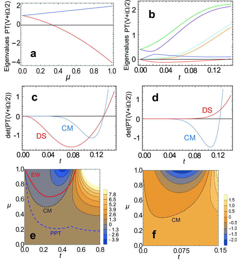
Figure 1: Covariance matrix detection of entanglement for spin systems. (a) Eigenvalues of the matrix (9) for the Werner-Bell state (10) with operators $\xi=\{\sigma_{A}^{x}\sigma_{B}^{x},\sigma_{A}^{y}\sigma_{B}^{y},\sigma_{A}^{z}\sigma_{B}^{z}\}$. (b) Eigenvalues, (c) determinant of the matrix (9) for the state (11) with $\mu=1$ and $M=20$ with operators (12). In (c), the covariance matrix (CM) result is compared to the Duan-Simon (DS) approach Duan ; simon . (d) Same as (c) but with using spin variables ${S^{x}}^{\prime}=(S^{x}+S^{y})/\sqrt{2},{S^{y}}^{\prime}=(S^{y}-S^{x})/\sqrt{2},{S^{z}}^{\prime}=S^{z}$. (e) The determinant of (9) for the mixed state (10) for the state (11) with $M=2$. The boundary for the PPT criterion and the entanglement witness (EW) is shown for comparison, where entanglement is detected above the line. (f) Same as (e) but for $M=20$.

We consider the scenario where only second order correlations of the total spin operators can be measured. The $N=6$ operators we consider are

$$\xi=(S^{x}_{A},S^{y}_{A},S^{z}_{A},S^{x}_{B},S^{y}_{B},S^{z}_{B}).$$ (12)

Similar to the qubit example considered above we find that only $(S^{y}_{B})^{T_{B}}=-S^{y}_{B}$ undergoes a sign change under a partial transpose, and other spin operators are invariant. The eigenvalue spectrum of the pure state (11) is given in Fig 1(b) for $M=20$. From our results we observe that there is one negative eigenvalue in the time range $0<t\lesssim 0.13$, thus in this case entanglement is detected only for a limited time range. This is expected as only second order correlations are used, not the full information of the density matrix. From the observation that there is only one negative eigenvalue, an equivalent method of detecting entanglement is to evaluate the determinant (the product of all eigenvalues) of the matrix (9), and test for positivity. The determinant approach is shown in Fig 1(c), where we observe that the same region of entanglement as shown in Fig 1(b) is detected.

We compare the performance of our method by performing a Holstein-Primakoff approximation where the spin operators are treated as approximate position and momentum operators $x_{A,B}\approx S^{y}_{A,B}/\sqrt{2M},p_{A,B}\approx S^{z}_{A,B}/\sqrt{2M}$. This can then be applied to continuous variable methods such as the criterion of Duan, Simon, and co-workers Duan ; simon . From the results in Fig 1(c), we find that the Duan-Simon criteria detects the same region of entanglement as our covariance method. This can be explained by the fact that when the operators are chosen to be field quadratures, our formulation reduces to Simon’s criterion (simon, ), and thus are equivalent. While we have a $6\times 6$ matrix rather than a $4\times 4$ in Simon’s criterion, the position and momentum operators $x_{A,B},p_{A,B}$ are already optimized for the correlations that are produced by the state, and the additional two operators do not add further information. On the other hand, the measured operators may be quite different from the optimal operators in an experiment, due to the incomplete knowledge of the state, or potential calibration errors. A quantum state is characterized in a typical experiment by measuring the various correlations between observables. In such cases another choice of operators $x_{A,B}^{\prime},p_{A,B}^{\prime}$ will then sub-optimally detect entanglement using the Duan-Simon approach as can be seen from Fig. 1(d). In contrast our criterion still continues to detect entanglement since no information of the optimal basis needs to be input to the covariance matrix. This comes about due to the symmetric set of operators (12) which span the same operator space under SO(3) rotations.

Turning to mixed states, a comparison between PPT criteria, our covariance matrix method and the entanglement witness method horedecki1996separability ; PhysRevA.62.052310 ; szangolies2015detecting ; singh2016entanglement for $M=2$ is shown in Fig. 1(e). The entanglement witness approach numerically optimizes a witness operator $W=\sum_{ij}c_{ij}a_{i}\otimes b_{i}$ over coefficients $c_{ij}$, where $a_{i},b_{i}\in\{I,S^{x}_{A,B},S^{y}_{A,B},S^{z}_{A,B}\}$ . We see that the covariance matrix method and the entanglement witness method detect a smaller region of entanglement in contrast to the PPT criterion. This is expected again because the PPT criterion uses the full density matrix, but the other two methods use only a limited set of correlators. We find that the covariance matrix method can detect entanglement in a larger region of the state space than the entanglement witness approach, and in particular is more efficient in detecting entanglement when the state is more mixed (i.e. smaller $\mu$). Further we notice that even for this small Hilbert space dimension $D=9$, computing the entanglement witness is numerically intensive, due to the constrained optimization involved in the procedure. This is in contrast to our method which requires evaluating a determinant of (9) which can be done in a time polynomially scaling with $N$.

For larger systems $M=20$, the covariance matrix method continues to detect entanglement for times in the region $0<t\lesssim 1/2\sqrt{M}$ jing18 . A comparison to the PPT criterion shows that to the accuracy of the plot the full range $0\lesssim\mu\leq 1$, $0<t\leq 0.15$ exhibits entanglement. The reason for the large region of entanglement is that for systems in a larger Hilbert space, the amount of entanglement is accordingly larger, and are of a form that is relatively robust byrnes2013 . Again the limited region of entanglement detection is the price to be paid of only the low order correlations. Despite the increased complexity of the state, our method continues to detects a large portion of the parameter space. We find that in this case the dimension of the Hilbert space already makes the entanglement witness method unreliable due to incomplete optimization. This is again due to the complexity of the optimization which scales with the Hilbert space dimension $D$, rather than the number of operators $N$ chosen.

V Conclusions

In summary, we have generalized the covariance matrix approach for detecting entanglement in bipartite systems. Our approach allows for an arbitrary number and type of operators to be used to form a covariance matrix. The symmetric formulation of the criteria (8) in terms of matrix invariances automatically takes into account of symmetries that are present in the problem. This means that it is not necessary to construct suitable observables that are sensitive to the particular entangled state that is being detected, and one can work in a basis-independent way. This suggests that the larger the number of observables that are included in the covariance matrix, better the chance of detecting the entanglement as it includes further correlations that may be relevant to entanglement. We expect that the most promising application of the approach will be to high dimensional systems where complete tomography of the state is impossible or impractical. In this case, one would like to detect entanglement using only partial information of the state, with a limited set of observables. Our method is highly efficient in the sense that the complexity of calculating the entanglement is related to the number of operators chosen $N$, rather than the dimension of the Hilbert space $D$. We expect that the system can be applied to many different systems beyond those explored here, such as in quantum many-body systems where only a limited number of correlation functions are available.

VI acknowledgments

We thank Bartosz Regula for motivating this work, and Jonathan Dowling, Yumang Jing for discussions. This work is supported by the Shanghai Research Challenge Fund; New York University Global Seed Grants for Collaborative Research; National Natural Science Foundation of China (61571301); the Thousand Talents Program for Distinguished Young Scholars (D1210036A); and the NSFC Research Fund for International Young Scientists (11650110425); NYU-ECNU Institute of Physics at NYU Shanghai; the Science and Technology Commission of Shanghai Municipality (17ZR1443600); and the China Science and Technology Exchange Center (NGA-16-001).

VII APPENDIX

VII.1 Symmetries of the matrices $V$ and $\Omega$

In this section we show the symmetry properties of the matrices $V$ and $\Omega$. We first show that $V$ is a real symmetric matrix:

$$V_{jk}^{*} =\frac{1}{2}\langle\{\Delta\xi_{j},\Delta\xi_{k}\}^{\dagger}\rangle$$

$$=\frac{1}{2}\langle\left(\Delta\Delta\xi_{k}^{\dagger}\Delta\xi_{j}^{\dagger}+\xi_{j}^{\dagger}\Delta\xi_{k}^{\dagger}\right)\rangle$$

$$=\frac{1}{2}\langle\{\Delta\xi_{j},\Delta\xi_{k}\}\rangle$$

$$=V_{jk}=V_{kj},$$ (13)

where we have used the fact that the chosen operators are Hermitian $\xi_{n}^{\dagger}=\xi_{n}$.

Next, we show that $\Omega$ is a real antisymmetric matrix:

$$\Omega_{jk}^{*} =i\langle[\xi_{j},\xi_{k}]^{\dagger}\rangle$$

$$=i\langle\left(\xi_{k}^{\dagger}\xi_{j}^{\dagger}-\xi_{j}^{\dagger}\xi_{k}^{\dagger}\right)\rangle$$

$$=i\langle[\xi_{k},\xi_{j}]\rangle$$

$$=-\Omega_{kj}=\Omega_{jk},$$ (14)

which proves the statement. We note that the matrices are defined in the $N\times N$ space of the chosen operators $\xi_{n}$, and not in the Hilbert space of the operators. Thus while the quantity $-i[\xi_{j},\xi_{k}]$ is Hermitian, the matrix $\Omega_{jk}$ is not.

It then follows that the quantity in (4) of the main text is a Hermitian matrix:

$$\left(V+\frac{i}{2}\Omega\right)^{\dagger}=V^{T}-\frac{i}{2}\Omega^{T}=V+\frac{i}{2}\Omega.$$ (15)

One can view $V$ as being the real part and $\Omega/2$ as being the imaginary parts of the Hermitian matrix.

VII.2 Validity of (4) for mixed states

In this section we show that (4) in the main text holds for mixed states. Taking a general mixed state

$$\rho=\sum_{l}p_{l}|\Psi_{l}\rangle\langle\Psi_{l}|,$$ (16)

and using the fact that

$$V_{jk}+\frac{i}{2}\Omega_{jk}=\langle\xi_{j}\xi_{k}\rangle-\langle\xi_{j}\rangle\langle\xi_{k}\rangle$$ (17)

we have

$$V_{jk}+\frac{i}{2}\Omega_{jk}= \sum_{l}p_{l}\langle\Psi_{l}|\xi_{j}\xi_{k}|\Psi_{l}\rangle$$

$$-\sum_{l}\sum_{l^{\prime}}p_{l}p_{l^{\prime}}\langle\Psi_{l}|\xi_{j}|\Psi_{l}\rangle\langle\Psi_{l^{\prime}}|\xi_{k}|\Psi_{l^{\prime}}\rangle.$$ (18)

Given a positive semi-definite matrix, all the principal submatrices are also positive semi-definite. Even though our operators $\xi_{i}$ do not form the complete basis in Hilbert space, they do correspond to one of the principal submatrices of the matrix formed by complete set of operators. This enables us to use Eq. (29) of Gittsovich et.al.gitts and the second term can be bounded as a matrix inequality in the labels $j,k$ as

$$V_{jk}+\frac{i}{2}\Omega_{jk} \geq\sum_{l}p_{l}\left(\langle\Psi_{l}|\xi_{j}\xi_{k}|\Psi_{l}\rangle-\langle\Psi_{l}|\xi_{j}|\Psi_{l}\rangle\langle\Psi_{l}|\xi_{k}|\Psi_{l}\rangle\right).$$ (19)

The quantity in the brackets is the pure state result as shown in (8) of the main text. Since this is a positive semi-definite matrix, the probabilistic sum can be bounded by zero, which yields (4) for mixed states.

VII.3 Generalized uncertainty relations

We start with defining a phase space vector $\xi=(\xi_{1},\xi_{2},..\xi_{N})$ such that

$$[\xi_{a},\xi_{b}]=i\Omega_{ab},$$ (20)

where $a,b=1,2,..N$. Here $\Omega_{ab}$ is the $N$ ${\times}$ $N$ dimensional commutation matrix. We give a general formalism for $N$ arbitrary operators $\{\hat{\xi}_{i}\}$. Defining

$$|f_{i}\rangle=(\hat{\xi_{i}}-\langle\hat{\xi_{i}}\rangle)|\Psi\rangle,$$ (21)

the variance in various operators is

$$\sigma^{2}_{i} =\langle\Psi|(\hat{\xi_{i}}-\langle{\hat{\xi_{i}}}\rangle)^{2}|\Psi\rangle=\langle{f_{i}}|f_{i}\rangle.$$ (22)

The product of all such operators is then given as

$$\prod_{i}\sigma^{2}_{i} =\prod_{i}\langle{f_{i}}|f_{i}\rangle.$$ (23)

Given a set of $N$ state vectors $\{|f_{i}\rangle;i=1,2,..,N\}$, we can use the Gram-Schmidt procedure arfken to obtain a set of $N$ orthogonal (but unnormalized) state vectors as

$$|f^{\perp}_{i}\rangle=|f_{i}\rangle-\sum_{j=1}^{i-1}\frac{\langle{f}^{\perp}_{j}|f_{i}\rangle}{\langle{f}^{\perp}_{j}|f^{\perp}_{j}\rangle}|f^{\perp}_{j}\rangle$$ (24)

Now using the positivity of norm of the orthogonal states, (23) gives for $N=1$

$$\sigma^{2}_{\xi_{1}}\geqslant 0.$$ (25)

For $N=2$, we use the Cauchy Schwarz inequality which is defined as

$$\langle{f_{1}}|f_{1}\rangle\langle{f_{2}}|f_{2}\rangle\geqslant|\langle{f_{1}}|f_{2}\rangle|^{2}$$ (26)

to obtain Schrodinger’s uncertainty relation,

$$\sigma^{2}_{\xi_{1}}\sigma^{2}_{\xi_{2}}\geqslant \mathinner{\!\left\lvert\frac{1}{2}\langle\{\hat{\xi_{1}},\hat{\xi_{2}}\}\rangle-\langle\hat{\xi_{1}}\rangle\langle\hat{\xi_{2}}\rangle\right\rvert}^{2}+\mathinner{\!\left\lvert\frac{1}{2i}\langle[\hat{\xi_{1}},\hat{\xi_{2}}]\rangle\right\rvert}^{2}$$ (27)

For $N=3$, we obtain the three operator uncertainty relation which in terms of the state vectors can be given as

$$\sigma^{2}_{\xi_{1}}\sigma^{2}_{\xi_{2}}\sigma^{2}_{\xi_{3}}\geqslant \langle{f_{1}}|f_{1}\rangle|\langle{f_{2}}|f_{3}\rangle|^{2}+\langle{f_{1}}|f_{2}\rangle\langle{f_{2}}|f_{3}\rangle\langle{f_{3}}|f_{1}\rangle$$

$$+\langle{f_{2}}|f_{2}\rangle|\langle{f_{3}}|f_{1}\rangle|^{2}+\langle{f_{2}}|f_{1}\rangle\langle{f_{3}}|f_{2}\rangle\langle{f_{1}}|f_{3}\rangle$$

$$+\langle{f_{3}}|f_{3}\rangle|\langle{f_{1}}|f_{2}\rangle|^{2}$$ (28)

which gives the expression in the main text.

VII.4 Entanglement witness approach

In this section we detail how to calculate the boundary as shown in Fig. 1(e) using an entanglement witness horedecki1996separability ; PhysRevA.62.052310 approach. The method we follow is an optimization approach as described in Ref. szangolies2015detecting . We assume the situation where only the correlations $\langle a_{i}\otimes b_{j}\rangle$ are available, where the operators on the $A$ and $B$ subsystems are

$$a_{i} \in\{I_{A},S_{A}^{x},S_{A}^{y},S_{A}^{z})$$

$$b_{i} \in\{I_{B},S_{B}^{x},S_{B}^{y},S_{B}^{z})$$ (29)

respectively. We then define the quantity

$$W=\sum_{ij=0}^{3}c_{ij}a_{i}\otimes b_{i}$$ (30)

where $c_{ij}$ are real coefficients. The procedure is then

$$\text{Minimize }\langle W\rangle\hskip 8.53581pt$$

Subject to: (1) $$W=P+Q^{T_{A}}$$

(2) $$P\geq 0$$

(3) $$Q\geq 0$$

(4) $$\text{Tr}(W)=1.$$ (31)

The only term with non-zero trace in (30) is the coefficient of $I_{A}\otimes I_{B}$, and the normalization condition is satisfied if

$$c_{00}=\frac{1}{(N+1)^{2}}.$$ (32)

The remaining coefficients $c_{ij}$ are found by a simulated annealing random search procedure.

References

- (1) Horodecki, R., Horodecki, P., Horodecki, M. & Horodecki, K. Quantum entanglement. Reviews of Modern Physics 81, 865 (2009).
- (2) Gühne, O. & Tóth, G. Entanglement detection. Physics Reports 474, 1–75 (2009).
- (3) Eisert, J., Brandão, F. G. & Audenaert, K. M. Quantitative entanglement witnesses. New Journal of Physics 9, 46 (2007).
- (4) Vedral, V. Quantifying entanglement in macroscopic systems. Nature 453, 1004–1007 (2008).
- (5) Plenio, M. B. & Virmani, S. An introduction to entanglement measures. arXiv preprint quant-ph/0504163 (2005).
- (6) Peres, A. Separability criterion for density matrices. Phys. Rev. Lett. 77, 1413–1415 (1996).
- (7) Horodecki, M., Horodecki, P. & Horodecki, R. Separability of mixed states: necessary and sufficient conditions. Physics Letters A 223, 1 – 8 (1996).
- (8) Horodecki, P. Separability criterion and inseparable mixed states with positive partial transposition. Physics Letters A 232, 333 – 339 (1997).
- (9) Plenio, M. B. Logarithmic negativity: A full entanglement monotone that is not convex. Phys. Rev. Lett. 95, 090503 (2005).
- (10) Vidal, G. & Werner, R. F. Computable measure of entanglement. Physical Review A 65, 032314 (2002).
- (11) Duan, L.-M., Giedke, G., Cirac, J. I. & Zoller, P. Inseparability criterion for continuous variable systems. Phys. Rev. Lett. 84, 2722–2725 (2000).
- (12) Hillery, M. & Zubairy, M. S. Entanglement conditions for two-mode states. Physical review letters 96, 050503 (2006).
- (13) Horedecki, M., Horodecki, P. & Horodecki, R. Separability of mixed states: necessary and sufficient conditions phys. Phys. Lett. A 223, 1–8 (1996).
- (14) Lewenstein, M., Kraus, B., Cirac, J. I. & Horodecki, P. Optimization of entanglement witnesses. Phys. Rev. A 62, 052310 (2000).
- (15) Szangolies, J., Kampermann, H. & Bruß, D. Detecting entanglement of unknown quantum states with random measurements. New Journal of Physics 17, 113051 (2015).
- (16) Singh, A., Dorai, K. et al. Entanglement detection on an nmr quantum-information processor using random local measurements. Physical Review A 94, 062309 (2016).
- (17) Spengler, C., Huber, M., Brierley, S., Adaktylos, T. & Hiesmayr, B. C. Entanglement detection via mutually unbiased bases. Phys. Rev. A 86, 022311 (2012).
- (18) Tóth, G. & Gühne, O. Detection of multipartite entanglement with two-body correlations. Applied Physics B 82, 237–241 (2006).
- (19) Laskowski, W. et al. Correlation-based entanglement criterion in bipartite multiboson systems. Phys. Rev. A 92, 022339 (2015).
- (20) Wu, L.-A., Bandyopadhyay, S., Sarandy, M. & Lidar, D. Entanglement observables and witnesses for interacting quantum spin systems. Physical Review A 72, 032309 (2005).
- (21) Jing, Y., He, Q. & Byrnes, T. Correlation-based entanglement criteria for bipartite systems. Phys. Rev. A 95, 052305 (2017).
- (22) de Vicente, J. I. & Huber, M. Multipartite entanglement detection from correlation tensors. Physical Review A 84, 062306 (2011).
- (23) Altepeter, J. et al. Experimental methods for detecting entanglement. Physical review letters 95, 033601 (2005).
- (24) Simon, R. Peres-horodecki separability criterion for continuous variable systems. Phys. Rev. Lett. 84, 2726–2729 (2000).
- (25) Braunstein, S. L. & van Loock, P. Quantum information with continuous variables. Rev. Mod. Phys. 77, 513 (2005).
- (26) Adesso, G. & Illuminati, F. Entanglement in continuous-variable systems: recent advances and current perspectives. Journal of Physics A: Mathematical and Theoretical 40, 7821 (2007).
- (27) Wang, X.-B., Hiroshima, T., Tomita, A. & Hayashi, M. Quantum information with gaussian states. Physics reports 448, 1–111 (2007).
- (28) Werner, R. F. & Wolf, M. M. Bound entangled gaussian states. Physical review letters 86, 3658 (2001).
- (29) Gühne, O. & Lütkenhaus, N. Nonlinear entanglement witnesses, covariance matrices and the geometry of separable states. In Journal of Physics: Conference Series, vol. 67, 012004 (IOP Publishing, 2007).
- (30) Devi, A. U., Uma, M., Prabhu, R. & Rajagopal, A. Constraints on the uncertainties of entangled symmetric qubits. Phys. Lett. A 364, 203–207 (2007).
- (31) Gittsovich, O., Gühne, O., Hyllus, P., Eisert, J. & Lvovsky, A. Covariance matrix criterion for separability. In AIP Conference Proceedings, vol. 1110, 63–66 (AIP, 2009).
- (32) Gühne, O., Hyllus, P., Gittsovich, O. & Eisert, J. Covariance matrices and the separability problem. Phys. Rev. Lett. 99, 130504 (2007).
- (33) Gittsovich, O. & Gühne, O. Quantifying entanglement with covariance matrices. Phys. Rev. A 81, 032333 (2010).
- (34) Li, M., Fei, S.-M. & Wang, Z.-X. Separability and entanglement of quantum states based on covariance matrices. Journal of Physics A: Mathematical and Theoretical 41, 202002 (2008).
- (35) Christensen, S. L. et al. Toward quantum state tomography of a single polariton state of an atomic ensemble. New Journal of Physics 15, 015002 (2013).
- (36) Lanyon, B. P. et al. Simplifying quantum logic using higher-dimensional hilbert spaces. Nature Physics 5, 134–140 (2009).
- (37) Gross, D., Liu, Y.-K., Flammia, S. T., Becker, S. & Eisert, J. Quantum state tomography via compressed sensing. Phys. Rev. Lett. 105, 150401 (2010).
- (38) Simon, R., Mukunda, N. & Dutta, B. Quantum-noise matrix for multimode systems: U( n ) invariance, squeezing, and normal forms. Phys. Rev. A 49, 1567–1583 (1994).
- (39) Szabo, A. & Ostlund, N. S. Modern quantum chemistry: introduction to advanced electronic structure theory (Courier Corporation, 2012).
- (40) Gittsovich, O., Gühne, O., Hyllus, P. & Eisert, J. Unifying several separability conditions using the covariance matrix criterion. Phys. Rev. A 78, 052319 (2008).
- (41) Nielsen, M. A. & Kempe, J. Separable states are more disordered globally than locally. Physical Review Letters 86, 5184 (2001).
- (42) Dalton, B., Heaney, L., Goold, J., Garraway, B. & Busch, T. New spin squeezing and other entanglement tests for two mode systems of identical bosons. New Journal of Physics 16, 013026 (2014).
- (43) Sørensen, A. S. & Mølmer, K. Entanglement and extreme spin squeezing. Phys. Rev. Lett. 86, 4431 (2001).
- (44) Korbicz, J., Cirac, J. I. & Lewenstein, M. Spin squeezing inequalities and entanglement of n qubit states. Phys. Rev. Lett. 95, 120502 (2005).
- (45) Byrnes, T. Fractality and macroscopic entanglement in two-component Bose-Einstein condensates. Phys. Rev. A 88, 023609 (2013).
- (46) Kurkjian, H., Pawłowski, K., Sinatra, A. & Treutlein, P. Spin squeezing and einstein-podolsky-rosen entanglement of two bimodal condensates in state-dependent potentials. Phys. Rev. A 88, 043605 (2013).
- (47) Burlak, G., Sainz, I. & Klimov, A. B. Entanglement enhancement for two spins assisted by two phase kicks. Phys. Rev. A 80, 024301 (2009).
- (48) Byrnes, T. et al. Macroscopic quantum information processing using spin coherent states. Optics Comm. 337, 102 – 109 (2015).
- (49) Ilo-Okeke, E. O. & Byrnes, T. Theory of single-shot phase contrast imaging in spinor Bose-Einstein condensates. Phys. Rev. Lett. 112, 233602 (2014).
- (50) Pyrkov, A. N. & Byrnes, T. New J. Phys. 16, 073038 (2014).
- (51) Giovannetti, V., Mancini, S., Vitali, D. & Tombesi, P. Characterizing the entanglement of bipartite quantum systems. Physical Review A 67, 022320 (2003).
- (52) Jing, Y., Fadel, M., Ivannikov, V., Treutlein, P. & Byrnes, T. Split spin-squeezed bose-einstein condensates. in preparation (2018).