The Early Stage of Molecular Cloud Formation by Compression of Two-phase Atomic Gases

Abstract

We investigate the formation of molecular clouds from atomic gas by using three-dimensional magnetohydrodynamic simulations, including non-equilibrium chemical reactions and heating/cooling processes. We consider super-Alfvénic head-on colliding flows of atomic gas possessing the two-phase structure that consists of HI clouds and surrounding warm diffuse gas. We examine how the formation of molecular clouds depends on the angle $\theta$ between the upstream flow and the mean magnetic field. We find that there is a critical angle $\theta_{\mathrm{cr}}$ above which the shock-amplified magnetic field controls the post-shock gas dynamics. If the atomic gas is compressed almost along the mean magnetic field ($\theta\ll\theta_{\mathrm{cr}}$), super-Alfvénic anisotropic turbulence is maintained by the accretion of the highly inhomogeneous upstream atomic gas. As a result, a greatly extended turbulence-dominated post-shock layer is generated. Around $\theta\sim\theta_{\mathrm{cr}}$, the shock-amplified magnetic field weakens the post-shock turbulence, leading to a dense post-shock layer. For $\theta\gg\theta_{\mathrm{cr}}$, the strong magnetic pressure suppresses the formation of cold dense clouds. Efficient molecular cloud formation is expected if $\theta$ is less than a few times $\theta_{\mathrm{cr}}$. Developing an analytic model and performing a parameter survey, we obtain an analytic formula for the critical angle as a function of the mean density, collision speed, and field strength of the upstream atomic gas. The critical angle is found to be less than $\sim 15^{\circ}$ as long as the field strength is larger than $1~{}\mu$G, indicating that the probability of occurrence of compression with $\theta<\theta_{\mathrm{cr}}$ is limited if shock waves come from various directions.

=1 The Friends of AASTeX Collaboration

1 Introduction

The formation of molecular clouds (MCs) is one of the fundamental building blocks in star formation. MCs are thought to form through shock compression of atomic gas. In galaxies, shock waves are frequently driven by several energetic phenomena, including supernova (SN) explosions (Chevalier, 1974; McKee & Ostriker, 1977; Koyama & Inutsuka, 2000), expansion of super-bubbles due to multiple SNe (McCray & Kafatos, 1987; Tomisaka et al., 1988; Dawson et al., 2011, 2013; Ntormousi et al., 2017), and galactic spiral waves (Wada et al., 2011; Grand et al., 2012; Baba et al., 2017).

Head-on colliding flows of warm neutral medium (WNM) have been considered to model the formation of MCs. The simple colliding flow model allows us to investigate the detailed physics working in the shocked regions using local numerical simulations with high resolution. Although the setup is simple, the shock compression generates a complex turbulent multi-phase structure consisting of shocked WNM and cold clouds condensed through the thermal instability (Koyama & Inutsuka, 2002; Audit & Hennebelle, 2005; Heitsch et al., 2005, 2006; Vázquez-Semadeni et al., 2006, 2007; Hennebelle & Audit, 2007; Hennebelle et al., 2007, 2008; Banerjee et al., 2009; Heitsch et al., 2009; Audit & Hennebelle, 2010; Vázquez-Semadeni et al., 2010, 2011; Clark et al., 2012). The turbulence is driven by various instabilities (Heitsch et al., 2008), including the thermal instability (Field, 1965; Balbus, 1986; Koyama & Inutsuka, 2000; Iwasaki & Tsuribe, 2008, 2009), the Kelvin-Helmholtz and Rayleigh-Taylor instabilities (Chandrasekhar, 1961), and the nonlinear thin-shell instability (Vishniac, 1994; Blondin & Marks, 1996; Heitsch et al., 2007; Folini et al., 2014). These simulation results successfully reproduce observational properties of the interstellar clouds (Hennebelle et al., 2007), such as the supersonic turbulence (Larson, 1979, 1981; Solomon et al., 1987; Heyer et al., 2009), the mass function of cold clumps (Kramer et al., 1998; Heithausen et al., 1998), and the angular correlation between filamentary atomic gases and magnetic fields (Clark et al., 2015; Inoue & Inutsuka, 2016).

Magnetic fields exert a great impact on the MC formation. Performing magnetohydrodynamic (MHD) simulations, Inoue & Inutsuka (2008, 2009) showed that interstellar clouds, which are the precursor of MCs, are formed only if the WNM is compressed almost along the magnetic field. Otherwise, the formation of dense clouds is prohibited by the shock-amplified magnetic field, and only HI clouds form (also see Hennebelle & Pérault, 2000; Heitsch et al., 2009; van Loo et al., 2010; Körtgen & Banerjee, 2015). If the WNM is compressed by shock waves from various directions with respect to magnetic fields, the MC formation is expected to be significantly delayed and HI clouds are formed in almost all compression events. Most simulations of the MC formation have focused on colliding flows parallel to the magnetic field (Hennebelle et al., 2008; Banerjee et al., 2009; Vázquez-Semadeni et al., 2011; Valdivia et al., 2016; Zamora-Avilés et al., 2018).

Although most authors have considered the MC formation directly from a typical atomic gas with a density of $\sim 1~{}\mathrm{cm}^{-3}$, there is some observational evidence that MCs grow through accretion of HI clouds with a density of $\sim 10~{}\mathrm{cm}^{-3}$ (Blitz et al., 2007; Fukui et al., 2009, 2017) and even through accretion of denser clouds containing molecules (Motte et al., 2014). In addition, recent global simulations of galaxies revealed that the direct precursor of MCs is not typical diffuse atomic gases but dense atomic gases with a mean density of $\sim 20~{}\mathrm{cm}^{-3}$ which have been piled up by dynamical disturbances (Dobbs et al., 2012; Bonnell et al., 2013; Baba et al., 2017). The formation of molecules requires a column density larger than $\sim 2\times 10^{21}~{}\mathrm{cm}^{-2}$ (van Dishoeck & Black, 1988). The accumulation length to form molecules is required to be larger than $650~{}\mathrm{pc}~{}(n/1~{}\mathrm{cm}^{-3})^{-1}$, where $n$ is the gas density (Hartmann et al., 2001; Pringle et al., 2001; McKee & Ostriker, 2007; Inoue & Inutsuka, 2009). This length may be too long to form MCs within a typical lifetime of a few tens of megayears estimated from observational results (Kawamura et al., 2009; Murray, 2011; Meidt et al., 2015). From the observational and theoretical points of view mentioned above, shock compression of gases denser than a typical atomic gas with a density of $\sim 1~{}\mathrm{cm}^{-3}$ is one plausible path from atomic gas to MCs. The dense atomic gases are generated by multiple episodes of shock compression (Inoue & Inutsuka, 2009; Inutsuka et al., 2015; Kobayashi et al., 2017, 2018).

Inoue & Inutsuka (2012) investigated the MC formation directly from collision of a dense atomic gas with a mean density of $\sim 5~{}\mathrm{cm}^{-3}$ along the magnetic field. They took into account the two-phase structure of the atomic gas (Field et al., 1969; Wolfire et al., 1995, 2003; Iwasaki & Inutsuka, 2014). They found that the collision of the highly inhomogeneous upstream gas drives super-Alfvénic anisotropic turbulence. MCs form on a timescale of $10$ Myr which is consistent with that estimated observationally by Kawamura et al. (2009).

Shock compression completely along the magnetic field considered in Inoue & Inutsuka (2012) is an extreme case. If the atomic gas is compressed from various directions randomly, shock compression misaligned to magnetic fields is more likely to occur. Although Hennebelle & Pérault (2000) and Inoue & Inutsuka (2009) have investigated the effect of field orientation on the cloud formation, their studies are restricted to the cases with colliding flows of the WNM with a density less than $1~{}\mathrm{cm}^{-3}$. Atomic gas intrinsically has the two-phase structure, and the resulting density inhomogeneity is expected to significantly affect the MC formation. In this paper, taking into account the realistic two-phase structure of atomic gas, we clarify how the MC formation depends on the angle between the upstream flow and magnetic field by performing three-dimensional magnetohydrodyamic simulations including simplified chemical reactions and cooling/heating processes.

This paper is organized as follows. Section 2 presents the basic equations, and methods for chemical reactions, heating/cooling processes, and simplified ray tracing. In Section 3, the results of a fiducial parameter set are presented. In Section 4, we introduce an analytic model that describes the simulation results. The results of a parameter survey are shown in Section 5. Astrophysical implications are discussed in Section 6. Finally, our results are summarized in Section 7.

2 Equations and Methods

2.1 Basic Equations

The basic equations are given by

$$\frac{\partial\rho}{\partial t}+\frac{\partial\left(\rho v_{\mu}\right)}{\partial x_{\mu}}=0,$$ (1)

$$\frac{\partial\rho v_{\mu}}{\partial t}+\frac{\partial}{\partial x_{\nu}}\left(\rho v_{\mu}v_{\nu}+T_{\mu\nu}\right)=0,$$ (2)

$$\frac{\partial E}{\partial t}+\frac{\partial}{\partial x_{\mu}}\left[\left(E\delta_{\mu\nu}+T_{\mu\nu}\right)v_{\nu}-\kappa\frac{\partial T}{\partial x_{\mu}}\right]=-{\cal L},$$ (3)

$$\frac{\partial B_{\mu}}{\partial t}+\frac{\partial}{\partial x_{\nu}}\left(v_{\nu}B_{\mu}-v_{\mu}B_{\nu}\right)=0,$$ (4)

and

$$T_{\mu\nu}=\left(P+\frac{B^{2}}{8\pi}\right)\delta_{\mu\nu}-\frac{B_{\mu}B_{\nu}}{4\pi},$$ (5)

where $\rho$ is the gas density, $v_{\mu}$ is the gas velocity, $B_{\mu}$ is the magnetic field, $E=\rho v^{2}/2+P/(\gamma-1)+B^{2}/8\pi$ is the total energy density, $T$ is the gas temperature, $\kappa$ is the thermal conductivity, and ${\cal L}$ is a net cooling rate per unit volume. The thermal conductivity for neutral hydrogen is given by $\kappa(T)=2.5\times 10^{3}~{}T^{1/2}$ cm^-1 K^-1 s^-1 (Parker, 1953).

Anisotropy of the thermal conduction is not important in our simulations because the ISM considered in this paper is weakly ionized. In the weakly ionized ISM, the main carriers of heat are neutral particles. The threshold temperature below which the effect of charged particles on the thermal conduction coefficient is negligible is approximately $5\times 10^{4}~{}\mathrm{K}$ (Parker 1953). In our simulations, the gas temperature increases to $\sim 10^{4}$ K through the shock compression and decreases due to radiative cooling, indicating that the gas temperature is lower than the threshold temperature throughout the computation box.

To solve the basic equations (1)-(4), we use Athena++ (Stone et al., 2019, in preparation) which is a complete rewrite of the Athena MHD code (Stone et al., 2008). The HLLD method is used as the MHD Riemann solver (Miyoshi & Kusano, 2005). Magnetic fields are integrated with the constrained transport method (Evans & Hawley, 1988; Gardiner & Stone, 2008).

Chemical reactions, heating/cooling processes, and ray tracing of far-ultraviolet (FUV) photons and cooling photons are newly implemented into Athena++ as shown in the next section. Because self-gravity is ignored in this paper, we focus on the early phase of the MC formation. The effect of self-gravity will be investigated in forthcoming papers.

2.2 Chemical Reactions and Heating/Cooling Processes

To treat the transition from atomic to molecular phases, non-equilibrium chemical reactions must be taken into account (Glover & Mac Low, 2007; Clark et al., 2012; Valdivia et al., 2016). We follow Inoue & Inutsuka (2012) for the chemical reactions, heating/cooling processes, and ray tracing of FUV and cooling photons. We reduce the number of chemical species, retaining H⁺, H, H₂, He⁺, He, and the most important species for cooling, C⁺, O, and CO. The elemental abundances of He, C, and O with respect to hydrogen nuclei are given by ${\cal A}_{\mathrm{He}}=0.1$, ${\cal A}_{\mathrm{C}}=1.5\times 10^{-4}$, and ${\cal A}_{\mathrm{O}}=3.2\times 10^{-4}$, respectively. In the formation of CO, we use a simplified treatment of the conversion of C⁺ to CO proposed by Nelson & Langer (1997). Glover & Clark (2012) showed that gas dynamics is not sensitive to the detailed chemistry, and the simplified method works reasonably well to capture the global behavior of the CO formation, although CO abundance is not very accurate. The FUV radiation field strength is set to $1.6\times 10^{-3}$ erg cm^-2 s^-1, corresponding to $G_{0}=1$ in the units of the Habing flux (Habing, 1968; Draine, 1978).

The detailed chemical reactions and cooling/heating processes are described in Inoue & Inutsuka (2012). One update is that the OI cooling is evaluated by using calculations of the populations of the three levels exactly.

The number density of the $i$th species, $n_{i}$, satisfies the following equation:

$$\frac{\partial n_{i}}{\partial t}+\frac{\partial\left(n_{i}v_{\mu}\right)}{\partial x_{\mu}}=F_{i}-D_{i},$$ (6)

where $F_{i}$ and $D_{i}$ are the formation and destruction rates of the $i$th species. The number density of electron is derived using charge neutrality, $n(e)=n(\mathrm{H}^{+})+n(\mathrm{He}^{+})+n(\mathrm{C}^{+})$. In this paper, the number density is referred to as that of hydrogen nuclei, $n=n(\mathrm{H})+n(\mathrm{H}^{+})+2n(\mathrm{H_{2}})$.

The density is given by

$$\rho=\sum_{i}m_{i}n_{i}=\mu m_{\mathrm{p}}n,$$ (7)

where $m_{i}$ is the mass of the $i$th species, $m_{\mathrm{p}}$ is the proton mass, and $\mu=1.4$ is the mean molecular weight. The equation of state is given by

$$P=n_{\mathrm{tot}}k_{\mathrm{B}}T,$$ (8)

where $n_{\mathrm{tot}}$ is the total number density of the gas particles, $n_{\mathrm{tot}}=\left(1+{\cal A}_{\mathrm{He}}+{\cal A}_{\mathrm{C}}+{\cal A}_{\mathrm{O}}\right)n+n(e)-n(\mathrm{H}_{2})-n(\mathrm{CO})$.

Since the timescale of the chemical reactions is much shorter than the dynamical and cooling timescales, a special treatment is required for solving the chemical reactions. We divide Equation (6) into the advection term and chemical reactions in an operation-splitting manner. First, we solve the advection of the chemical species coupled with equations (1)-(4). In order to keep consistency between equations (1) and (6) and to ensure the local conservation of the elemental abundances, we use the consistent multi-fluid advection algorithm (Plewa & Müller, 1999; Glover et al., 2010). After that the chemical reactions are solved. Inoue & Inutsuka (2008) and Inoue & Inutsuka (2012) developed the piecewise exact solution (PES) method. The PES method divides the chemical reactions into small sets of reactions, each of which has an analytic solution, and solves them in an operator-splitting manner. The advantage of the PES method is that iteration is not required. Comparing the results obtained using the PES method and an iterative implicit method with the Gauss-Seidel method, the difference is negligible at least in our simplified chemical network. Since the PES method takes a shorter calculation time than the iterative method, the PES method is adopted in this paper.

2.3 Initial and Boundary Conditions

As an initial condition, we prepare a two-phase atomic gas with a mean density of $\langle n_{0}\rangle$ as a precursor of MCs. To generate it, the following calculation is performed. A thermally unstable gas with a uniform density of $\langle n_{0}\rangle$ is set in a cubic simulation box of $(20~{}\mathrm{pc})^{3}$ in volume. We add a velocity perturbation that follows a power law with the Kolmogorov spectral index. There are two reasons why the Kolmogorov spectrum is used in the initial velocity dispersion. One is that Larson (1979) observationally discovered that there is a correlation between the velocity dispersion $\sigma$ of the atomic gas and the size of regions $l$, $\sigma=0.64~{}\mathrm{km~{}s^{-1}}\times(l/\mathrm{pc})^{0.37}$. The relation is quite similar to the Kolmogorov spectrum, which has the relation $\sigma\propto l^{1/3}$. The other is that the observed turbulence in the atomic gas is subsonic or transonic for the WNM. Theoretically, it is natural that subsonic turbulence follows the Kolmogorov spectrum, which is satisfied in incompressible turbulence. The spectrum of the initial velocity dispersion relates to the size distribution of the clumps of cold neutral medium (CNM), which may affect the efficiency of converting the upstream kinetic energy into the post-shock kinetic energy. The initial velocity dispersion is 10% of the initial sound speed. The initial magnetic field ${\bf B}_{0}$ is set to be uniform. The field strength is denoted by $B_{0}$, and the angle between ${\bf B}_{0}$ and the $x$-axis is denoted by $\theta$. Imposing periodic boundary conditions in all directions, we solve the basic equations until $t=8~{}$Myr which corresponds to several times of the cooling time of the initial unstable gas. In this calculation, we consider the optically thin cooling/heating processes and chemical reactions by ignoring the dust extinction and optical depth of the cooling photons. To save the computational time, the calculation is performed with a resolution of $128^{3}$.

Next we set an initial condition for the simulation of MC formation using the two-phase atomic gas obtained using the calculation shown above. The calculation domain is doubled in the $x$-direction, indicating that the volume is $(40~{}\mathrm{pc})\times(20~{}\mathrm{pc})^{2}$. The physical quantities are copied periodically in the $x$-direction. Fig. 1 shows the density slice at the $z=0$ plane of the initial condition for $\langle n_{0}\rangle=5~{}$cm^-3, $B_{0}=5~{}\mu$G, $\theta=45^{\circ}$, and $V_{0}=20$ km s^-1. A colliding flow profile $v_{x}(x,y,z)=-V_{0}\tanh(x/(1~{}\mathrm{pc}))$ is added in the initial profile. The Dirichlet boundary conditions are imposed at $x=\pm 20~{}$pc in a manner such that the initial distribution is continuously injected into the calculation domain with constant velocities of $V_{0}$ and $-V_{0}$ from $x=20~{}\mathrm{pc}$ and $x=-20~{}\mathrm{pc}$, respectively. Periodic boundary conditions are imposed at the $y$- and $z$-boundaries. The simulations are conducted on uniform $1024\times 512\times 512$ cells, leading to a grid size of 0.04 pc.

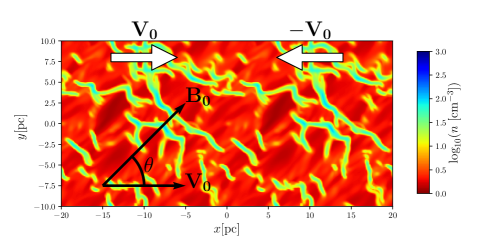
Figure 1: An example of the initial conditions: density cross section at the $z=0$ plane of the initial condition for $\langle n_{0}\rangle=5~{}$cm^-3, $B_{0}=5~{}\mu$G, and $\theta=45^{\circ}$

2.4 Methods for Estimating Column Densities and Optical Depths

In order to calculate the FUV flux at an arbitrary point, we need to integrate the column density along every ray path from the boundaries of the simulation box, summing over the contributions from each path. Since the exact radiation transfer is computationally expensive, a two-ray approximation in the $x$-direction is used (Inoue & Inutsuka, 2012). The FUV irradiation is calculated with two rays, which irradiate in the $x$-direction from the $x$-boundaries, $x=\pm 20$ pc. The flux of each ray is $G_{0}=0.5$. This approximation is justified by the geometry of the MC formation site. The compressed region has a sheet-like configuration extended in the $(y,z)$ plane. FUV photons penetrate mainly in the $x$-direction because the column densities in the $x$-direction are smaller than those along the $y$- and $z$-directions in the sheet structures.

The values of the local visual extinction at $(x,y,z)$ measured from the $x=20$ pc and $x=-20$ pc are given by

$$A_{\mathrm{V}}^{-}(x,y,z)=\frac{1}{N_{0}}\int_{-L}^{x}n(x^{\prime},y,z)dx^{\prime}\;\;\;$$ (9)

and

$$A_{\mathrm{V}}^{+}(x,y,z)=\frac{1}{N_{0}}\int_{x}^{L}n(x^{\prime},y,z)dx^{\prime},$$ (10)

respectively, where $N_{0}=1.9\times 10^{21}$ cm^-2 and $L=20$ pc.

The local column densities of C, H₂, and CO used in the chemical reactions and heating/cooling processes are calculated in a manner similar to that used in calculating the visual extinction. The two-ray approximation is also used for for the escape probabilities of the [OI] and [CII] cooling photons. The escape probabilities are calculated as follows: we estimate $\tau^{+}$ and $\tau^{-}$, which are the optical depths integrated from the left and right boundaries, respectively,

$$\tau^{\pm}(\mathrm{C^{+}},\mathrm{O})=\frac{N^{\pm}(\mathrm{C^{+}},\mathrm{O})}{N_{\tau}\delta v_{5}},$$ (11)

where $N_{\tau}=2.6\times 10^{17}~{}\mathrm{cm}^{-2}$ for the [OI] line and $N_{\tau}=1.5\times 10^{17}~{}\mathrm{cm}^{-2}$ for the [CII] line (Hollenbach & McKee, 1989), and $\delta v_{5}=\delta v/(1~{}\mathrm{km~{}s^{-1}})$ represents the Doppler shift effect. The OI and CII cooling processes are important in relatively low-density regions where the velocity dispersion along the $x$-direction is as high as $\sim 8$ km s^-1. Thus, $\delta v_{5}=8$ is adopted. The escape probability is evaluated as $\beta(\tau^{+})+\beta(\tau^{-})$, in which $\beta(\tau)$ is the escape probability in a semi-infinite medium (de Jong et al., 1980). The optical depth of the CO line cooling is evaluated in a similar way, but $\delta v_{5}=3$ is used because the high-density regions where CO forms have lower velocity dispersions.

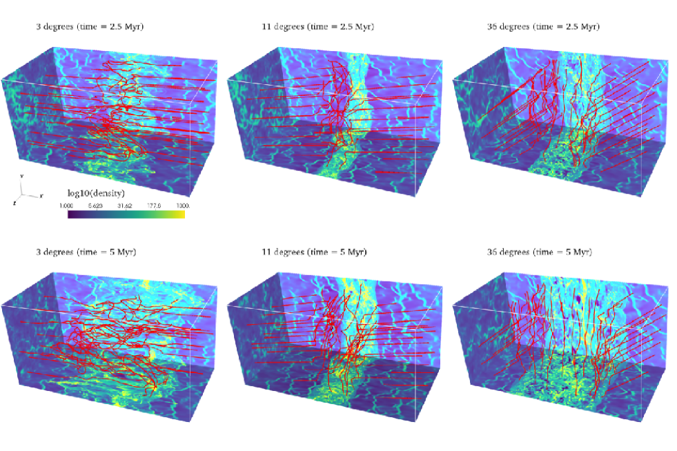
Figure 2: Density slices at the three orthogonal planes for $\Theta 3$ (left column), $\Theta 11$ (middle column), and $\Theta 36$ (right column). The upper and lower panels correspond to the results at $t=2.5$ Myr and $t=5$ Myr. The magnetic field lines are plotted as the red lines.

3 Results of a Fiducial Parameter Set

In this section, we investigate how the MC formation depends on $\theta$ in the fiducial model with a parameter set of $\langle n_{0}\rangle=5~{}\mathrm{cm}^{-3}$, $V_{0}=20$ km s^-1, $B_{0}=5~{}\mu$G. Super-shells are often observed as HI shells that have expansion speeds of $\sim 10-20~{}$km s^-1 and sizes of a few hundred parsecs (Heiles, 1979). Shock compressions with a velocity difference of $2V_{0}=40$ km s^-1 are expected in super-shells younger than $10~{}$Myr (McCray & Kafatos, 1987). The fiducial parameter set is motivated by collisions between adjacent expanding HI shells. Our setups are also relevant to the large-scale converging flows with a speed of a few tens of km s^-1 associated with the spiral arm formation (Wada et al., 2011). The field strength $B_{0}=5~{}\mu$G is close to the median value $\sim 6~{}\mu$G measured by observations of the Zeeman effect in CNM (Heiles & Troland, 2005; Crutcher et al., 2010). The median field strength is roughly consistent with other observations (Beck, 2001). Note that the median field strength of $\sim 6~{}\mu$G is not necessarily the most probable one since the probability distribution function (PDF) of the field strength is only loosely constrained by observations in the range $0<B_{0}<12~{}\mu$G. We explore the parameter space of ($\langle n_{0}\rangle$, $V_{0}$, $B_{0}$) in Section 5.

The upstream atomic gas has a two-phase structure as shown in Fig. 1. In this paper, we define WNM as the gas with a temperature higher than $10^{3}$ K. Typical densities of the CNM clumps and WNM are $\sim 40~{}\mathrm{cm}^{-3}$ and $\sim 2~{}\mathrm{cm}^{-3}$, respectively, indicating that the density contrast is as large as $\sim 20$. The density of the CNM is consistent with observations (Heiles & Troland, 2003). In our initial conditions, the CNM clumps make up roughly half of the total mass. Note that the warm gas, which we call WNM, is not in thermal equilibrium but still in a thermally unstable state. Indeed, observations have revealed that a substantial fraction of the atomic gas is in the unstable regime (Heiles & Troland, 2003; Kanekar et al., 2003; Roy et al., 2013). Theoretically, it is easy for the WNM to deviate from the thermal equilibrium state due to turbulence because the cooling/heating timescales are long (Gazol et al., 2001; Audit & Hennebelle, 2005). The Mach numbers of the colliding flow with respect to the WNM and CNM are $\sim 4$ and $\sim 18$, respectively. The Alfvén Mach number of the colliding flow for the WNM is $\sim 3$, while that for the CNM is $\sim 14$.

The results of three main models are shown: one is the case of an almost parallel field of $\theta=3^{\circ}$ which provides almost the same results as in the case of a completely parallel field case in Inoue & Inutsuka (2012), and the others are cases of oblique field in which the magnetic fields are tilted at $\theta=11^{\circ}$ and $36^{\circ}$ to the upstream flow. We name a model by attaching “$\Theta$” in front of a value of $\theta$ in degrees, i.e., models $\Theta 3$, $\Theta 11$, and $\Theta 36$.

A head-on colliding flow produces two shock fronts that propagate outward. The simulations are terminated at $t=5~{}$Myr because the shock fronts reach the $x$-boundaries for model $\Theta 3$. The termination time ($t=5$ Myr) is longer than the cooling times, which are approximately 1 Myr for the shocked warm gas and $10^{-2}$ Myr for the shocked CNM clumps (Equation (A3)). The termination time will be compared with the dynamical time in Section 3.3.

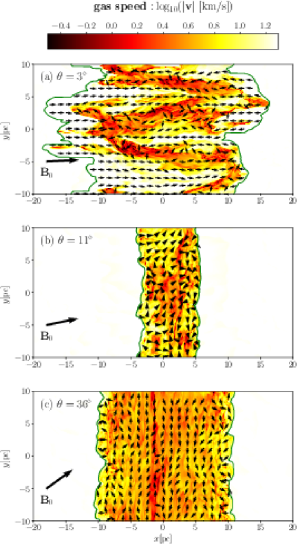
Figure 3: Gas speed slices in the $z=0$ plane at $t=5$ Myr for models (a) $\Theta 3$, (b) $\Theta 11$, and (c) $\Theta 36$. The velocity field is shown by the arrows only inside the post-shock layer. The two shock fronts whose positions are defined by the minimum and maximum of the $x$ coordinates where $P(x,y,z)/k_{\mathrm{B}}>5.8\times 10^{3}~{}\mathrm{K\cdot cm^{-3}}$ is satisfied. The positions of the identified shock fronts are shown by the green lines.

3.1 Main Features

Fig. 2 shows the density color maps in the three orthogonal planes at $t=2.5$ Myr and $t=5$ Myr for models $\Theta 3$, $\Theta 11$, and $\Theta 36$. The magnetic field lines are shown by the red lines. Unlike in WNM colliding flows, the CNM clumps exist in the upstream gas in the present models. A CNM clump is not decelerated completely when passing through a shock front, and plows the post-shock gas with a large $x$-momentum. The MHD interaction with the surrounding gas decelerates the CNM clump.

For model $\Theta 3$, since the CNM clumps move almost along the magnetic field, the Lorentz force does not contribute to their deceleration of the CNM clumps significantly. A CNM clump that enters into the post-shock layer from one of the shock fronts is not decelerated completely, and it collides with the shock front on the opposite side. Since the upstream CNM clumps accrete onto the post-shock layer from both the $\pm x$-directions, the shocked CNM clumps are moving in opposite directions along the $x$-axis in the post-shock layer. This ballistic-like motion of the CNM clumps pushes the shock fronts outward and significantly deforms them as shown in Fig. 2. The gas motion significantly widens the post-shock layer. These behaviors have been found by Inoue & Inutsuka (2012) and Carroll-Nellenback et al. (2014, without magnetic fields).

Note that if there were no radiative cooling, the CNM clumps would be quickly destroyed and mixed with the surrounding warm gas after passing through the shock fronts as shown in Klein et al. (1994). In our simulations, the radiative cooling, high density contrast, and magnetic fields extend the lifetime of the CNM clumps. The CNM clumps even grow through accretion of the surrounding warm gas due to radiative cooling. A detailed discussion is given in Appendix A.

The deformation of the shock fronts allows the kinetic energy of the upstream gas to remain almost unchanged after passing through them. The remaining kinetic energy is available to disturb the deep interior of the post-shock layer. Fig. 3a shows the gas velocity slice at the $z=0$ plane. The green lines indicate the two shock fronts whose positions are defined as the minimum and maximum of the $x$ coordinates where $P(x,y,z)/k_{\mathrm{B}}\geq P_{\mathrm{th}}$ is satisfied, where $P_{\mathrm{th}}$ is a threshold pressure that should be larger than the upstream mean pressure $P_{0}\sim 4.0\times 10^{3}$ K cm^-3. A value of $5.8\times 10^{3}$ K cm^-3 is adopted. We confirmed that the results are not sensitive to the choice of $P_{\mathrm{th}}$ as long as $P_{\mathrm{th}}$ is not far from $P_{0}$. In this figure, channel-flow-like fast WNM streams are visible in the post-shock layer. They are almost aligned to the $x$-axis, and their speeds are as fast as 10 km s^-1 which is comparable to the WNM sound speed. The CNM clumps are entrained by interaction with the surrounding warm gas, forming a filamentary structure elongated along the $x$-axis (also see Mellema et al., 2002; Cooper et al., 2009).

Magnetic fields are passively bent because the gas motion is super-Alfvénic, as will be shown in Section 3.2. The CNM clumps moving in opposite directions stretch the field lines preferentially in the direction of collision. As a result, the field lines are folded (Fig. 2). There are regions where the magnetic fields are flipped from the original orientation (Inoue & Inutsuka, 2012).

The middle column of Fig. 2 demonstrates that the small obliqueness of $\theta=11^{\circ}$ drastically changes the post-shock structure. Since the shock compression amplifies the tangential component of the magnetic field, the field lines are preferentially aligned to the $y$-axis although they have significant fluctuations. Since the shock-amplified tangential magnetic field pulls the CNM clumps back, they are decelerated before reaching the opposite side of the post-shock layer. The decelerated CNM clumps are accumulated in the central region. Unlike for model $\Theta 3$, there is no significant gas motion across the thickness of the post-shock layer (Fig. 3b). The post-shock layer therefore becomes much thinner than that for model $\Theta 3$.

When the magnetic field is further tilted at $\theta=36^{\circ}$ to the upstream flow, the results are almost the same as those for model $\Theta 11$ but the post-shock layer is thicker for model $\Theta 36$ (Fig. 2c). This is simply because it contains larger magnetic fluxes.

3.2 Transversely Averaged Momentum Flux in the Compression Direction

Figs. 2 and 3 suggest that the magnetic field controls the post-shock structures if the angle $\theta$ is large enough. To investigate the role of the magnetic fields in the post-shock structures quantitatively, we measure the momentum flux along the $x$-axis, which consists of the ram pressure ($P_{\mathrm{ram}}\equiv\rho v_{x}^{2}$), magnetic stress ($\Pi_{\mathrm{mag}}\equiv(B_{y}^{2}+B_{z}^{2}-B_{x}^{2})/8\pi$), and thermal pressure ($P_{\mathrm{th}}$). Note that the magnetic stress $\Pi_{\mathrm{mag}}$ is not the magnetic pressure but the $xx$ component of the Maxwell stress tensor. Since the magnetic tension contributes to $\Pi_{\mathrm{mag}}$, $\Pi_{\mathrm{mag}}$ can be negative if the magnetic tension is larger than the magnetic pressure. These quantities are useful for understanding quantitatively which pressures are dominant in the post-shock layers.

The transversely volume-weighted averaged momentum fluxes, which are denoted by $\langle P_{\mathrm{ram}}\rangle_{yz}$, $\langle\Pi_{\mathrm{mag}}\rangle_{yz}$, and $\langle P_{\mathrm{th}}\rangle_{yz}$, are plotted in Fig. 4 as functions of $x$ at two different epochs, of $t=2.5$ Myr and $t=5$ Myr for models $\Theta 3$, $\Theta 11$, and $\Theta 36$. In all the models, the transversely averaged total momentum flux ($\langle P_{\mathrm{tot}}\rangle_{yz}=\langle P_{\mathrm{ram}}\rangle_{yz}+\langle\Pi_{\mathrm{mag}}\rangle_{yz}+\langle P_{\mathrm{th}}\rangle_{yz}$) almost coincides with the upstream ram pressure $\langle\rho_{0}\rangle V_{0}^{2}$, indicating that the pressure balance is established along the $x$-axis. This implies that the average propagation speed of the shock fronts is negligible in the computation frame. Indeed, the average shock propagation speed along the $x$-axis is only a few km s^-1 in the computation frame, and hence the shock velocity with respect to the upstream gas does not differ from $V_{0}$ by more than $\sim 10$%.

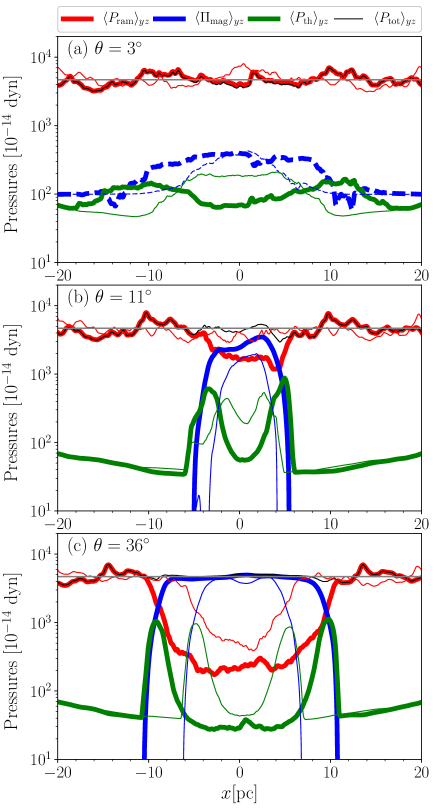
Figure 4: Transversely averaged $P_{\mathrm{ram}}$ (red), $\Pi_{\mathrm{mag}}$ (blue), and $P_{\mathrm{th}}$ (green) for models (a) $\Theta 3$, (b) $\Theta 11$, and (c) $\Theta 36$. The thin and thick lines represent the results at $t=2.5$ Myr and $t=5$ Myr, respectively. The blue dashed line shows that $\Pi_{\mathrm{mag}}$ is negative, indicating that the magnetic tension is larger than the magnetic pressure. The total pressures are shown by the black lines only at $t=5$ Myr. The horizontal gray line corresponds to the ram pressure of the atomic gas $\langle\rho_{0}\rangle V_{0}^{2}$.

For model $\Theta 3$, $\langle P_{\mathrm{ram}}\rangle_{yz}$ is much larger than the other pressures throughout the post-shock layer, regardless of time. This clearly shows that the gas motion is highly supersonic and super-Alfvénic. The transversely averaged magnetic stress $\langle\Pi_{\mathrm{mag}}\rangle_{yz}$ is always negative, or $\langle B_{x}^{2}\rangle>\langle B_{y}^{2}+B_{z}^{2}\rangle$ because the parallel component of the magnetic field is preferentially amplified by the channel-like fast gas flows biased in the collision direction (Fig. 3a). Amplification of the transverse field component does not work significantly.

For the oblique field models ($\Theta 11$ and $\Theta 36$), the post-shock layers can be divided into two regions. One is the warm surface layer, where all the pressures contribute equally to the total momentum flux. The other is the cold central layer, where $\langle P_{\mathrm{th}}\rangle_{yz}$ is low while $\langle\Pi_{\mathrm{mag}}\rangle_{yz}$ is high. A similar two-region structure was also found in WNM colliding flows perpendicular to the magnetic field (Heitsch et al., 2009).

The warm surface layers are formed by a continuous supply of the upstream WNM. After shock heating, it cools down by radiative cooling, and accretes onto the cold central layer. Thus, the thicknesses of the warm surface layers are roughly determined by the cooling length; this is estimated to be 2 pc, which is comparable to their thicknesses in Fig. 4. When a CNM clump enters the post-shock layer, it passes through a warm surface layer easily and collides with the cold central layer.

In the cold central layer, $\langle P_{\mathrm{ram}}\rangle_{yz}$ decreases with time both for models $\Theta 11$ and $\Theta 36$. This is because the cold central layer is “shielded” by the tangential magnetic field shown in Fig. 2 against the accretion of the CNM clumps. This accretion of the CNM clumps disturbs the gas near the surfaces of the cold central layer. The turbulence inside the cold central layer decays due to numerical dissipation and escaping cooling photons from the shock-heated regions, leading to a decrease in $\langle P_{\mathrm{ram}}\rangle_{yz}$ in the central layer. The time evolution of $\langle\Pi_{\mathrm{mag}}\rangle_{yz}$ in the central layer is different between models $\Theta 11$ and $\Theta 36$. For model $\Theta 11$, at $t=2.5$ Myr, $\langle P_{\mathrm{ram}}\rangle_{yz}$ plays an important role in the total pressure. Thus, the decrease in $\langle P_{\mathrm{ram}}\rangle_{yz}$ causes the post-shock layer to become denser, leading to an increase in $\langle\Pi_{\mathrm{mag}}\rangle_{yz}$ due to flux freezing (Fig. 4b). By contrast, for model $\Theta 36$, the post-shock layer is mainly supported by the magnetic stress at $t=2.5$ Myr. Since $\langle P_{\mathrm{ram}}\rangle_{yz}$ makes a negligible contribution to the pressure balance where $\langle\Pi_{\mathrm{mag}}\rangle_{yz}\sim\langle\rho_{0}\rangle V_{0}^{2}$, $\langle\Pi_{\mathrm{mag}}\rangle_{yz}$ is constant with time in the cold central layer (Fig. 4c).

3.3 Velocity Dispersion

In Section 3.2, we found that the ram pressure does not decrease for model $\Theta 3$ while it decreases with time for the oblique field models ($\Theta 11$ and $\Theta 36$). In this section, we examine the time evolution of the post-shock velocity dispersion.

Fig. 5 shows the mass-weighted and CO-density-weighted velocity dispersions, which are measured along the $x$-axis ($\delta v_{x}$) and averaged between the $y$- and $z$-components ($\delta v_{yz}\equiv\sqrt{(\delta v_{y}^{2}+\delta v_{z}^{2})/2}$) for models $\Theta 3$, $\Theta 11$, and $\Theta 36$. The CO-density-weighted velocity dispersions correspond to the velocity dispersions in the dense regions where $n>10^{3}~{}\mathrm{cm}^{-3}$ because CO forms only in the dense regions as shown in Section 6.3.

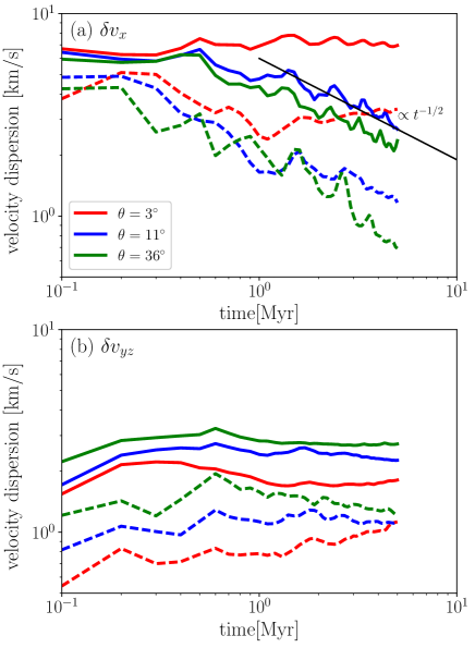
Figure 5: Time evolution of the mass-weighted (solid lines) and CO-density-weighted (dashed lines) velocity dispersions for models $\Theta 3$ (red), $\Theta 11$ (blue), and $\Theta 36$ (green). The top and bottom panels represent the velocity dispersions parallel to the $x$-axis and those averaged in the $y$- and $z$-components, $\delta v_{yz}\equiv\sqrt{(\delta v_{y}^{2}+\delta v_{z}^{2})/2}$, respectively. Equation (13) is shown by the black line in the top panel.

We investigate how many dynamical timescales are considered in the simulations. The dynamical time depends on the direction. In the $x$-direction, the dynamical time is given by $t_{\mathrm{dyn},x}=L_{x}/\delta v_{x}$, where $L_{x}$ is the width of the post-shock layer. By measuring $L_{x}$ from Fig. 3 and $\delta v_{x}$ from Fig. 5a at $t=5$ Myr, one obtains $t_{\mathrm{dyn},x}\sim 3~{}$Myr for models $\Theta 3$ and $\Theta 11$, and $6.5$ Myr for model $\Theta 36$. Thus, the post-shock gases are mixed well on the $x$-axis for models $\Theta 3$ and $\Theta 11$. The dynamical times with respect to the transverse direction are given by $({20~{}\mathrm{pc}})/\delta v_{yz}\sim 8~{}\mathrm{Myr}$ where $\delta v_{yz}$ is set to 2.5 km s^-1 from Fig. 5b for all the models. The simulations are terminated before the transverse dynamical time.

First, we examine the velocity dispersion parallel to the $x$-axis. Fig. 5a shows that in the early phase ($t<0.5~{}$Myr), $\delta v_{x}$ is as high as $6-7~{}$km s^-1. Fig. 6 indicates that $\delta v_{x}(t=0.5~{}\mathrm{Myr})$ is almost independent of $\theta$ although there are fluctuations. The efficiency $\epsilon$ for converting the kinetic energy of the upstream atomic gas into the post-shock kinetic energy parallel to the collision direction is expressed as

$$\epsilon\equiv\frac{\dot{M}_{\mathrm{tot}}t\delta v_{x}^{2}/2}{\dot{M}_{\mathrm{tot}}tV_{0}^{2}/2}=\left(\frac{\delta v_{x}}{V_{0}}\right)^{2}\sim 10\%,$$ (12)

where $\dot{M}_{\mathrm{tot}}=2\langle\rho_{0}\rangle V_{0}L^{2}$ is the mean mass accretion rate. Fig. 7 illustrates that the time evolution of the total post-shock kinetic energies parallel to the $x$-axis, which increase obeying $(\epsilon\dot{M}_{\mathrm{tot}}V_{0}^{2}/2)t$ for all the models in the early phase, where $\epsilon=10\%$. The efficiency $\epsilon=10\%$ is larger than those obtained from simulations considering WNM colliding flows (Heitsch et al., 2009; Körtgen & Banerjee, 2015; Zamora-Avilés et al., 2018). The upstream two-phase structure enhances the efficiency.

For $t>0.5$ Myr, we find a clear dependence of $\delta v_{x}$ on $\theta$ from Fig. 5a. The velocity dispersion parallel to the $x$-axis is almost constant or even slightly increases with time at least until $5$ Myr for model $\Theta 3$, while it decreases with time for models $\Theta 11$ and $\Theta 36$.

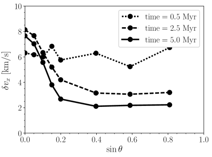
Figure 6: The velocity dispersions parallel to the $x$-axis measured at the three different epochs $t=0.5~{}$Myr (dotted), $t=2.5$ Myr (dashed), and $t=5~{}$Myr (solid) are plotted as a function of $\sin\theta$.

Why does $\delta v_{x}$ not decrease for model $\Theta 3$? One reason is that the gas flows are not fully turbulent, but rather laminar as shown in Fig. 3a. The gas flows are strongly biased in the collision direction, and the transverse motion is restricted ($\delta v_{yz}/\delta v_{x}\sim 0.3$ in Figs. 5a and 5b). Since translational coherent gas flow is unlikely to decay, $\delta v_{x}$ does not decrease.

Interestingly, for both of the models $\Theta 11$ and $\Theta 36$, the velocity dispersions parallel to the $x$-axis are closely approximated by

$$\delta v_{x}\sim\delta v_{x0}(t/t_{0})^{-1/2},$$ (13)

where $\delta v_{x0}=6~{}\mathrm{km~{}s^{-1}}$ and $t_{0}=1~{}\mathrm{Myr}$ although $\delta v_{x}$ is slightly smaller for model $\Theta 36$ than for model $\Theta 11$. In order to see the universality of the time evolution of $\delta v_{x}$ more clearly, we investigate the $\theta$-dependence of $\delta v_{x}$ using additional simulations with different field orientations. Fig. 6 shows $\delta v_{x}$ at the three different epochs as a function of $\sin\theta$. At both $t=2.5$ Myr and at $t=5~{}$Myr, $\delta v_{x}$ shows a decrease in the range of $0^{\circ}<\theta<11^{\circ}$, and the decreases suddenly slow down around $\theta\sim 11^{\circ}$. For angles larger than $\theta\sim 11^{\circ}$, $\delta v_{x}$ does not depend on $\theta$ sensitively.

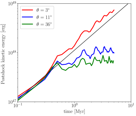
Figure 7: Time evolution of the total post-shock kinetic energies parallel to the $x$-axis for models $\Theta 3$ (red), $\Theta 11$ (blue), and $\Theta 36$ (green). The black line indicates the time evolution of the post-shock kinetic energy in the case where the fraction $\epsilon=10~{}\%$ of the upstream kinetic energy is converted into the post-shock kinetic energy $(\epsilon\dot{M}_{\mathrm{tot}}V_{0}^{2}/2)t$.

The time dependence of $\delta v_{x}\propto t^{-1/2}$ implies that the total kinetic energy parallel to the $x$-axis ($\dot{M}_{\mathrm{tot}}t\delta v_{x}^{2}/2$) is constant with time. Fig. 7 indicates that the total post-shock kinetic energies parallel to the $x$-axis are constant with time in the late phase ($t>0.5~{}$Myr) for models $\Theta 11$ and $\Theta 36$. This is probably explained if the rate of kinetic energy input from the shock fronts balances with dissipation rates.

The transverse velocity dispersion $\delta v_{yz}$ shows the opposite trend to $\delta v_{x}$; $\delta v_{yz}$ is larger for larger $\theta$ although the difference is small. The reason why model $\Theta 3$ gives the lowest $\delta v_{yz}$ is that the motion of the CNM clumps is not randomized in the post-shock layer (Fig. 3a). In contrast to $\delta v_{x}$, $\delta v_{yz}$ does not decrease even for models $\Theta 11$ and $\Theta 36$. There are several mechanisms to drive transverse velocity dispersion. Especially for larger angles (e.g., model $\Theta 36$), the presence of an upstream field component perpendicular to the collision direction drives a transverse flow behind the shock front following the MHD Rankine-Hugoniot relation (de Hoffmann & Teller, 1950). The transverse flow is generated even without any perturbation. In Fig. 3c, the gas is moving coherently in the $+y$-direction for $x<0$ and in the $-y$-direction for $x>0$. As long as a colliding flow is stationary, the transverse flow speed should remain approximately constant. Another mechanism is that the shock-amplified magnetic field bends the gas motion so that the gas flow is parallel to the transverse direction (Heitsch et al., 2009). The shock deformation due to the accretion of the CNM clumps generates a transverse flow along the magnetic field (Inoue & Fukui, 2013; Inoue et al., 2018). The thermal instability that develops preferentially along the magnetic field (Field, 1965) also contributes to the transverse velocity dispersion.

For all the models, the CO-density-weighted velocity dispersions are larger than $1$ km s^-1, indicating that the velocity dispersions in the cold dense gases are supersonic with respect to their sound speeds ($\sim 0.3~{}$km s^-1). Collision of the two-phase atomic gas drives stronger post-shock turbulence than that of the WNM (Inoue & Inutsuka, 2012; Carroll-Nellenback et al., 2014).

3.4 Mean Post-shock Densities

Fig. 8 shows the time evolution of the mean post-shock densities $\langle n_{\mathrm{sh}}\rangle$ which are derived by averaging densities over the identified post-shock layers.

In the early phase ($t<0.5~{}\mathrm{Myr}$), the mean post-shock densities are enhanced only by a factor of 8 and are comparable among the models because the super-Alfvénic collision of the inhomogeneous atomic gas drives strong velocity dispersions, regardless of $\theta$ (Fig. 5a).

Fig. 8 shows that only model $\Theta 11$ exhibits a rapid increase in $\langle n_{\mathrm{sh}}\rangle$ while the mean post-shock densities retain their initial values for the other models. For model $\Theta 11$, the obliqueness is large enough for the cold central layer to develop, but it is small enough for $\langle P_{\mathrm{ram}}\rangle$ to be a main contributor to the support of the post-shock layer against the upstream ram pressure. Thus, the decrease in $\langle P_{\mathrm{ram}}\rangle$ causes the post-shock layer to become denser, leading to the increase in $\langle n_{\mathrm{sh}}\rangle$. For model $\Theta 3$ ($\Theta 36$), the ram pressure (magnetic stress) suppresses further gas compression.

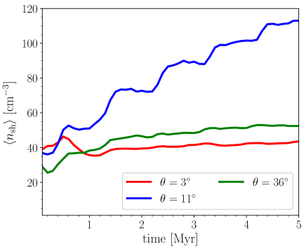
Figure 8: Time evolution of the mean post-shock densities for models $\Theta 3$ (red), $\Theta 11$ (blue), and $\Theta 36$ (green).

3.5 Density PDFs and Dense Gas Fractions

We found that the mean post-shock densities increase only for model $\Theta 11$ from Fig. 8. In the MC formation, how much dense gas forms is important because molecules are preferentially formed in dense gases. In this section, we investigate the density PDFs and the time evolution of the mass fraction of dense gases.

3.5.1 Density PDFs

The mass-weighted density probability distribution functions (PDFs) ${\cal P}$ are shown in Fig. 9 for models $\Theta 3$, $\Theta 11$, and $\Theta 36$. The definition of ${\cal P}$ is given by

$${\cal P}(X_{i})=\frac{1}{M_{\mathrm{tot}}\Delta X}\int_{|X-X_{i}|<\Delta X/2}\rho d^{3}x,$$ (14)

where $X\equiv\log_{10}n$ is divided into equally spaced bins whose widths are denoted by $\Delta X$, $i$ is the index of the bins, and $M_{\mathrm{tot}}=\dot{M}_{\mathrm{tot}}t$ is the total mass of the post-shock layer. At $t=2.5$ Myr, the PDFs for all the models have log-normal shapes, although the PDF for model $\Theta 11$ is slightly shifted toward higher densities than for the other PDFs. Therefore, model $\Theta 11$ has the highest mean density (Fig. 8).

For models $\Theta 3$ and $\Theta 36$, the PDFs show little time variation, as in the time evolution of $\langle n_{\mathrm{sh}}\rangle$ found in Fig. 8, although the high-density tails are slightly extended toward higher densities.

By contrast, model $\Theta 11$ shows significant time variation not only in $\langle n_{\mathrm{sh}}\rangle$ but also in the PDF. Interestingly, even without self-gravity, Fig. 9 shows that the mass fraction of the dense gas with $n>10^{3}~{}\mathrm{cm}^{-3}$ significantly increases with time. This implies that the gas is compressed not only in the collision direction but also along the field lines. The increase in $f_{>10^{3}}$ is caused by transverse flows generated behind a shock front and by gas condensation due to the thermal instability that tends to develop along magnetic fields (Field, 1965).

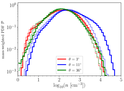
Figure 9: Mass-weighted probability distribution functions (PDFs) of gas density for models $\Theta 3$ (red), $\Theta 11$ (blue), and $\Theta 36$ (green). For each of the models, the thin and thick lines correspond to the results at $t=2.5$ Myr and $t=5$ Myr, respectively.

3.5.2 Time Evolution of Dense Gas Mass Fractions

To investigate the evolution of dense gases more clearly, we measure the mass fractions of the dense gases with $n>10^{2}~{}\mathrm{cm}^{-3}$ and $n>10^{3}~{}\mathrm{cm}^{-3}$, which are denoted by $f_{>10^{2}}$ and $f_{>10^{3}}$, respectively.

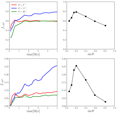
Figure 10: Time evolution of the mass fraction of dense gases with $n>10^{2}~{}\mathrm{cm}^{-3}$ (the top left panel) and with $n>10^{3}~{}\mathrm{cm}^{-3}$ (the bottom left panel). In both panels, the red, blue, and lines correspond to the results for models $\Theta 3$, $\Theta 11$, and $\Theta 36$, respectively. The mass fraction of dense gases with $n>10^{2}~{}\mathrm{cm}^{-3}$ (the top right panel) and $n>10^{3}~{}\mathrm{cm}^{-3}$(the bottom right panel) at $t=5~{}$Myr as a function of $\sin\theta$.

The top left panel of Fig. 10 shows the time evolution of $f_{>10^{2}}$ for models $\Theta 3$, $\Theta 11$, and $\Theta 36$. In all the models $f_{>10^{2}}$ does not depend on time sensitively. The dense gas mass with $n>10^{2}~{}\mathrm{cm}^{-3}$ increases at a constant rate.

Note that the fractional difference in $f_{>10^{2}}$ is only $30\%$ among the models, although $\langle n_{\mathrm{sh}}\rangle$ for model $\Theta 11$ is more than twice as large as than those for models $\Theta 3$ and $\Theta 36$ (Fig. 8). This indicates that the post-shock layers for models $\Theta 3$ and $\Theta 36$ contain wider and less-dense regions than model $\Theta 11$ while the total masses with $n>10^{2}~{}\mathrm{cm}^{-3}$ are comparable.

Using the results with various field orientations shown in Fig. 6, we plot $f_{>10^{2}}$ at $t=5$ Myr as a function of $\sin\theta$ in the top right panel in Fig. 10. The figure exhibits a weak $\theta$-dependence of $f_{>10^{2}}$. The mass fraction has a broad peak around $\theta\sim 11^{\circ}~{}(\sin\theta\sim 0.2)$ which gives the maximum mean density in Fig. 8.

By contrast, the mass fraction of denser gas ($n>10^{3}~{}\mathrm{cm}^{-3}$) is sensitive to $\theta$. The time evolution of the mass fraction of the dense gas with $n>10^{3}~{}\mathrm{cm}^{-3}$ is plotted in the bottom left panel of Fig. 10. While $f_{>10^{3}}$ is constant with time for models $\Theta 3$ and $\Theta 36$, $f_{>10^{3}}$ increases rapidly with time for model $\Theta 11$. This rapid increase is related to the development of the high-density tail in the density PDF for model $\Theta 11$ (Fig. 9).

The bottom right panel of Fig. 10 shows that $f_{>10^{3}}$ at $5~{}\mathrm{Myr}$ has a sharp peak around $\theta\sim 10^{\circ}$ $(\sin\theta\sim 0.2)$. For angles larger (smaller) than $\sim 10^{\circ}$, $f_{>10^{3}}$ rapidly decreases because of the magnetic stress (ram pressure).

3.6 The Formation of Molecules

At $t=5$ Myr, the mean accumulated column density reaches $2\langle n_{0}\rangle V_{0}t\sim 3.2\times 10^{21}~{}\mathrm{cm}^{-2}$, corresponding to a mean visual extinction of $2\langle n_{0}\rangle V_{0}t/N_{0}\sim 1.6$. Thus, H₂ and CO are expected to form in regions where FUV photons are shielded. For H₂, the self-shielding is effective if column densities of H₂ are larger than $\sim 10^{14}~{}$$\mathrm{cm}^{-2}$ (Draine & Bertoldi, 1996). Thus almost all the regions in the post-shock layers are self-shielded. By contrast, the formation of CO proceeds only when $A_{\mathrm{V}}$ exceeds unity, because it requires dust extinction.

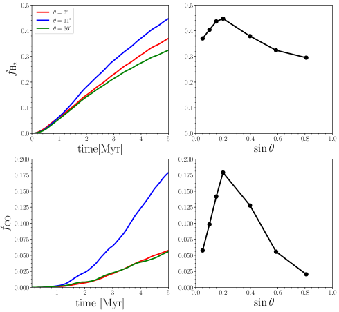
Figure 11: Time evolution of the H₂ fraction (the top left panel) and CO fraction (the bottom left panel) in the post-shock layers. In both panels, the red, blue, and green lines correspond to the results for models $\Theta 3$, $\Theta 11$, and $\Theta 36$, respectively. The H₂ fraction (the top right panel) and CO fraction (the bottom right panel) at $t=5~{}$Myr are plotted as functions of $\sin\theta$.

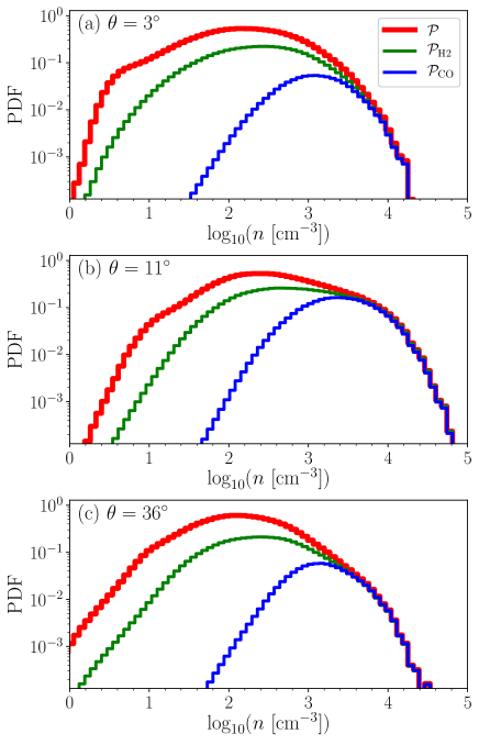
Figure 12: Mass-weighted probability distribution function of gas density (red lines) for the models (a) $\Theta 3$, (b) $\Theta 11$, and (c) $\Theta 36$. The green and blue lines indicate the H₂-density-weighted (${\cal P}_{\mathrm{H_{2}}}$) and CO-density-weighted (${\cal P}_{\mathrm{CO}}$) PDFs of gas density, respectively. In all the panels, the PDFs are calculated at $t=5$ Myr.

3.6.1 Formation of hydrogen molecules

The top left panel of Fig. 11 shows the time evolution of the mass fraction of H₂ in the accreted hydrogen nuclei, which is defined as

$$f_{\mathrm{H_{2}}}\equiv\frac{\displaystyle\int 2n(\mathrm{H_{2}})d^{3}x}{2\langle n_{0}\rangle V_{0}L^{2}t}.$$ (15)

The mass fraction of H₂ increases continuously with time, and the increase in $f_{\mathrm{H_{2}}}$ is faster for model $\Theta 11$ than for models $\Theta 3$ and $\Theta 36$. Although the self-shielding is effective, the H₂ formation on dust grains takes a relatively long time. A typical formation time of H₂ in the gas with a density of $n$ is estimated from $t_{\mathrm{form,H_{2}}}=(k_{\mathrm{H_{2}}}n)^{-1}\sim 15~{}\mathrm{Myr}\left(n/10^{2}~{}\mathrm{cm}^{-3}\right)^{-1}$, where $k_{\mathrm{H_{2}}}\sim 2\times 10^{-17}~{}\mathrm{cm^{3}~{}s^{-1}}$ is the H₂ formation rate assuming that the gas and dust temperatures are 100 K and 10 K, respectively (Hollenbach & McKee, 1979). Glover & Mac Low (2007) and Valdivia et al. (2016) reported that the density inhomogeneity promotes the H₂ formation because $t_{\mathrm{H_{2}}}$ is shorter for denser gases. In order to investigate the effect of the density inhomogeneity on the H₂ formation, we estimate an H₂ fraction by assuming that the post-shock layer has a spatially and temporally constant density of $n$. In the derivation of the H₂ fraction, we take into account the effect of mass accretion, which continuously supplies H₂-free atomic gas into the post-shock layer. The detailed derivation is presented in Appendix B. We obtain the H₂ fraction at $t_{\mathrm{f}}=5~{}$Myr which is given by

$$f_{\mathrm{H_{2},ave}}(n)=1-\frac{1-e^{-2k_{\mathrm{H_{2}}}nt_{\mathrm{f}}}}{2k_{\mathrm{H_{2}}}nt_{\mathrm{f}}}.$$ (16)

For model $\Theta 11$, $\langle n_{\mathrm{sh}}\rangle$ increases from $\sim 40~{}\mathrm{cm}^{-3}$ to $\sim 115~{}\mathrm{cm}^{-3}$ (Fig. 8). Thus, the H₂ fraction derived assuming the spatially constant post-shock density of $\langle n_{\mathrm{sh}}\rangle$ is expected to take a value between $f_{\mathrm{H_{2},ave}}(40~{}\mathrm{cm}^{-3})=0.1$ and $f_{\mathrm{H_{2},ave}}(115~{}\mathrm{cm}^{-3})=0.3$. For models $\Theta 3$ and $\Theta 36$, $\langle n_{\mathrm{sh}}\rangle$ remains a value of $\sim 40~{}\mathrm{cm}^{-3}$ from Fig. 8, leading to $f_{\mathrm{H_{2},ave}}(40~{}\mathrm{cm}^{-3})\sim 0.1$. Thus for all the models, the formation of H₂ proceeds faster than predicted by $f_{\mathrm{H_{2},ave}}(n=\langle n_{\mathrm{sh}}\rangle)$.

The comparison of $f_{\mathrm{H_{2}}}(t=t_{\mathrm{f}})$ with $f_{\mathrm{H_{2},ave}}$ suggests that the rapid formation of H₂ arises from the high density-inhomogeneity in the post-shock layers. In order to examine which density ranges are responsible for the H₂ formation, we plot the H₂-density-weighted PDFs $P_{\mathrm{H_{2}}}$ calculated at $t=5$ Myr for the three models in Fig. 12. $P_{\mathrm{H_{2}}}$ is defined by

$${\cal P}_{\mathrm{H_{2}}}(X_{i})=\frac{\displaystyle\int_{|X-X_{i}|<\Delta X/2}2\mu n(\mathrm{H_{2}})m_{\mathrm{H}}d^{3}x}{M_{\mathrm{tot}}\Delta X}.$$ (17)

For reference, the mass-weighted PDFs of gas density ${\cal P}$ are plotted in Fig. 12. If ${\cal P}_{\mathrm{H_{2}}}$ coincides with ${\cal P}$ at a density bin, all the hydrogen nuclei become H₂ in the corresponding density range. Fig. 12 illustrates that the formation of H₂ depends on density. The H₂ fraction is almost unity in the gas with a density larger than $10^{3}~{}\mathrm{cm}^{-3}$. This is because $t_{\mathrm{H_{2}}}(n>10^{3}~{}\mathrm{cm}^{-3}$) is less than $1.5$ Myr which is sufficiently short to form H₂. The density giving $t_{\mathrm{form,H_{2}}}=5~{}$Myr is approximately $300~{}\mathrm{cm}^{-3}$ which corresponds to the peak densities of ${\cal P}_{\mathrm{H_{2}}}$ for all the panels of Fig. 12.

The top right panel of Fig. 11 shows the $\theta$-dependence of $f_{\mathrm{H_{2}}}$ at $t=5$ Myr. The mass fraction of $\mathrm{H_{2}}$ does not depend on $\theta$ sensitively, and there is a broad peak around $\theta=11^{\circ}$. Even in models $\Theta 3$ and $\Theta 36$ having low $\langle n_{\mathrm{sh}}\rangle$, the H₂ fractions are comparable to that in model $\Theta 11$. The weak $\theta$-dependence of $f_{\mathrm{H_{2}}}$ comes from the fact that the H₂ formation occurs mainly in the dense gas with $n>10^{2}~{}\mathrm{cm}^{-3}$ whose mass fraction exhibits a weak $\theta$-dependence as shown in Fig. 10.

3.6.2 Formation of CO

Fig. 12 shows the CO-density-weighted PDFs of gas density ${\cal P}_{\mathrm{CO}}$ which is defined as

$${\cal P}_{\mathrm{CO}}(X_{i})=\frac{\displaystyle\int_{|X-X_{i}|<\Delta X/2}\mu n(\mathrm{CO})m_{\mathrm{H}}d^{3}x}{{\cal A}_{\mathrm{C}}M_{\mathrm{tot}}\Delta X}.$$ (18)

If ${\cal P}_{\mathrm{CO}}$ coincides with ${\cal P}$ in a bin, all the carbon nuclei are in the form of CO in the corresponding density range. Fig. 12 shows that CO formation proceeds preferentially in denser gases than H₂ formation. For $n<10^{3}~{}\mathrm{cm}^{-3}$, the CO fractions quickly decrease as density decreases for all the models because CO molecules are destroyed by FUV photons for low-density regions where $A_{\mathrm{V}}<1$.

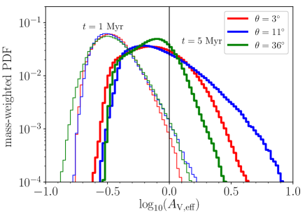
Figure 13: Mass-weighted probability distribution function of the effective visual extinction for the models $\Theta 3$ (red), $\Theta 11$ (blue), and $\Theta 36$ (green). The results at $t=1$ Myr and $t=5$ Myr are shown by the thin and thick lines for each model, respectively. The vertical line indicates $A_{\mathrm{V,eff}}=1$ above which dust extinction works effectively.

The bottom left panel of Fig. 11 shows the time evolution of the mass fraction of CO in the accreted C-bearing species, which is defined as

$$f_{\mathrm{CO}}=\frac{\int n(\mathrm{CO})d^{3}x}{2\langle n_{0}\rangle{\cal A}_{\mathrm{C}}V_{0}L^{2}t}.$$ (19)

The CO fractions remain extremely small in the early phase and begin to increase at points near $t\sim 1~{}$Myr for all the models (the bottom left panel of Fig. 11). This behavior of $f_{\mathrm{CO}}$ can be roughly understood from the time evolution of dust extinction. In order to characterize the dust extinction at each position, we define the effective visual extinction $A_{\mathrm{V,eff}}$ as

$$A_{\mathrm{V,eff}}=-\frac{1}{2.5}\ln\left[\frac{1}{2}\left(e^{-2.5A_{\mathrm{V}}^{-}}+e^{-2.5A_{\mathrm{V}}^{+}}\right)\right],$$ (20)

where the factor of $2.5$ comes from the dust extinction factor $e^{-2.5A_{\mathrm{V}}}$ of the CO photodissociation rate (Glover et al., 2010). In the initial conditions, the mean values of $A_{\mathrm{V,eff}}$ in the simulation box are 0.16 and their maximum values are $0.32$ for all the models, indicating that dust extinction does not work initially and the CO abundances are extremely low. As the atomic gas accumulates into the post-shock layer, the mean value of $A_{\mathrm{V,eff}}$ increases with time. In addition, spatial variations of $A_{\mathrm{eff}}$ are enhanced by shock compression. Fig. 13 shows the PDFs of $A_{\mathrm{eff}}$ in the post-shock layers for models $\Theta 3$, $\Theta 11$, and $\Theta 36$. Around $t=1$ Myr, the high $A_{\mathrm{V,eff}}$ tails of the PDFs start to exceed $A_{\mathrm{V,eff}}=1$ for all the models (Fig. 13). This indicates that the regions shielded by dust grains are formed at a epoch near $t\sim 1$ Myr. At that epoch, $f_{\mathrm{CO}}$ begins to grow (the bottom-left panel of Fig. 11).

Unlike the H₂ formation, the CO formation proceeds more rapidly for model $\Theta 11$ than for models $\Theta 3$ and $\Theta 36$. This is because the gas tends to have higher $A_{\mathrm{V,eff}}$ for model $\Theta 11$ than for models $\Theta 3$ and $\Theta 36$ as shown in the PDFs at $t=5~{}$Myr in Fig. 13. In addition, model $\Theta 11$ has a larger amount of the dense gas with $n>10^{3}~{}\mathrm{cm}^{-3}$ (Fig. 9). An increase in gas density promotes the CO formation.

Note that the fraction of CO is still less than 20% even for model $\Theta 11$ because we terminate the simulations at the relatively early epoch of $t=5~{}$Myr to ignore self-gravity. The CO formation is expected to proceed and a significant fraction of the gas will be fully molecular after $t=5~{}$Myr. The later evolution will be discussed in Section 6.

4 An Analytical Model Describing Time Evolution of the Post-shock Layers

Our results showed that there is a critical angle denoted by $\theta_{\mathrm{cr}}$ above which the shock-amplified magnetic field controls the post-shock layers. We define the critical angle $\theta_{\mathrm{cr}}$ as the angle above which the velocity dispersion parallel to the $x$-axis obeys $\delta v_{x0}(t/t_{0})^{-1/2}$. From Figs. 5a and 6, the critical angle is set to $11^{\circ}$ in the fiducial parameter set. In Sections 3.2-3.4, we found that the time evolution of the post-shock layer can be understood using the pressure balance between the pre- and post-shock gases. In this section, we establish a simple analytic model that describes the global time evolution of the post-shock layers.

4.1 Formulation

The pressure balance between the post- and pre-shock gases is given by

$$\langle P_{\mathrm{ram}}\rangle_{\mathrm{ana}}+\langle\Pi_{\mathrm{mag}}\rangle_{\mathrm{ana}}\sim\langle\rho_{0}\rangle V_{0}^{2},$$ (21)

where $\langle P_{\mathrm{ram}}\rangle_{\mathrm{ana}}\equiv\langle\rho_{\mathrm{sh}}\rangle\delta v_{x}^{2}$, $\langle\Pi_{\mathrm{mag}}\rangle_{\mathrm{ana}}=B_{\mathrm{sh\perp}}^{2}/8\pi$, and $B_{\mathrm{sh\perp}}$ is the mean transverse field strength. The effect of the parallel field component is omitted in Equation (21) because $V_{0}$ is super-Alfvénic. The effect of the radiative cooling is implicitly considered by ignoring the thermal pressure in Equation (21). The contribution of the thermal pressure to the total momentum flux is negligible for all the models (Fig. 4). The magnetic flux conservation across a shock front is given by

$$\frac{B_{\mathrm{sh\perp}}}{\langle\rho_{\mathrm{sh}}\rangle}=\frac{B_{0}\sin\theta}{\langle\rho_{0}\rangle}.$$ (22)

Combining Equation (21) with (22), one obtains

$$\frac{\langle\rho_{\mathrm{sh}}\rangle}{\langle\rho_{0}\rangle}=-\left(\frac{\delta v_{x}}{C_{\mathrm{A0\perp}}}\right)^{2}+\sqrt{\left(\frac{\delta v_{x}}{C_{\mathrm{A0\perp}}}\right)^{4}+2\left(\frac{V_{0}}{C_{\mathrm{A0\perp}}}\right)^{2}}$$ (23)

where $C_{\mathrm{A0\perp}}=B_{0}\sin\theta/\sqrt{4\pi\langle\rho_{0}\rangle}$ is the upstream Alfvén speed with respect to the transverse component of the upstream magnetic field.

Equations (21)-(23) imply that $\delta v_{x}$ is related to the post-shock structure. The ram pressure becomes equal to the magnetic stress when the velocity dispersion satisfies $\delta v_{x}=\delta v_{x,\mathrm{eq}}$, where

$$\delta v_{x,\mathrm{eq}} = \sqrt{\frac{V_{0}C_{\mathrm{A0\perp}}}{2}}$$ (24)

$$= 2.9~{}\mathrm{km~{}s^{-1}}~{}\left(\frac{V_{0}}{20~{}\mathrm{km~{}s^{-1}}}\right)^{1/2}\left(\frac{B_{0}\sin\theta}{5~{}\mu\mathrm{G}\times\sin 11^{\circ}}\right)^{1/2}$$

$$\hskip 85.35826pt\times\left(\frac{\langle n_{0}\rangle}{5~{}\mathrm{cm}^{-3}}\right)^{-1/4}$$

If $\delta v_{x}\gg\delta v_{x,\mathrm{eq}}$, the ram pressure dominates over the magnetic stress. In this case, Equation (23) is reduced to $\langle\rho_{\mathrm{sh}}\rangle/\langle\rho_{0}\rangle\sim\left(V_{0}/\delta v_{x}\right)^{2}$. If $\delta v_{x}\ll\delta v_{x,\mathrm{eq}}$, mainly the magnetic stress supports the post-shock layers. In this case, the mean post-shock density is given by

$$\frac{\langle\rho_{\mathrm{sh}}\rangle}{\langle\rho_{0}\rangle}\sim\frac{\langle\rho_{\mathrm{sh}}\rangle_{\mathrm{m}}}{\langle\rho_{0}\rangle}\equiv\frac{V_{0}\sqrt{8\pi\langle\rho_{0}\rangle}}{B_{0}\sin\theta}.$$ (25)

Equation (25) was derived by McKee & Hollenbach (1980) and Inoue & Inutsuka (2009).

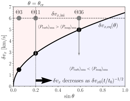
Figure 14: The critical velocity dispersion $\delta v_{x,\mathrm{eq}}$ for which the ram pressure is equal to the magnetic stress as a function of $\sin\theta$ (black solid line). The red and blue regions correspond to the $\langle P_{\mathrm{ram}}\rangle_{\mathrm{ana}}$-dominated and $\langle\Pi_{\mathrm{mag}}\rangle_{\mathrm{ana}}$-dominated regions, respectively. The velocity dispersion parallel to the $x$-axis in the very early phase is plotted as the horizontal dashed line. The dotted vertical line corresponds to the critical angle below which the turbulence is maintained. The three gray circles indicate the velocity dispersions in the early phases for models $\Theta 3$, $\Theta 11$, and $\Theta 36$. The velocity dispersions giving equality for models $\Theta 3$, $\Theta 11$, and $\Theta 36$ are shown by the three black circles. The gray arrows represent the time evolutions of $\delta v_{x}$ for the models until $t=5~{}$Myr.

Fig. 14 shows $\delta v_{x,\mathrm{eq}}$ as a function of $\sin\theta$. If $\delta v_{x}$ is larger (smaller) than $\delta v_{x,\mathrm{eq}}$, $\langle P_{\mathrm{ram}}\rangle_{\mathrm{ana}}$ ($\langle\Pi_{\mathrm{mag}}\rangle_{\mathrm{ana}}$) dominates in the post-shock layers. Let us consider the time evolution of the post-shock layers in this figure. In the early phase, the super-Alfvénic collision of the high density-inhomogeneous gas drives the longitudinal velocity dispersion as large as $\sim 6~{}$km s^-1 (the horizontal dashed line), regardless of $\theta$ (Fig. 5). The later evolution of $\delta v_{x}$ is determined by the critical angle of $\theta_{\mathrm{cr}}$ (the vertical dotted line). If $\theta$ is less than $\theta_{\mathrm{cr}}$, $\delta v_{x}$ does not decrease with time and remains the initial value of $\sim 6$ km s^-1. As long as $\theta\geq\theta_{\mathrm{cr}}$, we found that $\delta v_{x}$ decreases as $v_{x0}(t/t_{0})^{-1/2}$, regardless of $\theta$ as in Figs. 5a and 6. The gray arrows indicate the time evolutions of $\delta v_{x}$ until $t=5$ Myr for models $\Theta 11$ and $\Theta 36$. Fig. 14 clearly shows that the magnetic stress overtakes the ram pressure earlier for model $\Theta 36$ than for model $\Theta 11$ since the difference between $\delta v_{x}(t)$ and $\delta v_{x,\mathrm{eq}}$ indicates the significance of the ram pressure.

The analytic formula for the time evolution of $\delta v_{x}$ (Equation (13)) allows us to express Equations (21)-(23) as a function of time. At a given $\theta$, $\langle P_{\mathrm{ram}}\rangle_{\mathrm{ana}}$ becomes equal to $\langle\Pi_{\mathrm{mag}}\rangle_{\mathrm{ana}}$, and $\delta v_{x}$ reaches $\delta v_{x,\mathrm{eq}}$ when $t=t_{\mathrm{eq}}$, where

$$t_{\mathrm{eq}} = 4.4~{}\mathrm{Myr}\left(\frac{\delta v_{x0}/V_{0}}{0.3}\right)^{2}\left(\frac{V_{0}}{20~{}\mathrm{km~{}s^{-1}}}\right)$$ (26)

$$\hskip 28.45274pt\left(\frac{\langle n_{0}\rangle}{5~{}\mathrm{cm}^{-3}}\right)^{1/2}\left(\frac{B_{0}\sin\theta}{5~{}\mu\mathrm{G}\times\sin 11^{\circ}}\right)^{-1}.$$

4.2 Comparison with the Simulation Results

4.2.1 Mean Magnetic Stresses

Fig. 15 shows $\langle\Pi_{\mathrm{mag}}\rangle$ measured at $t=2.5$ Myr and $t=5~{}$Myr as a function of $\sin\theta$. The ram pressures are not plotted because $\langle P_{\mathrm{ram}}\rangle+\langle\Pi_{\mathrm{mag}}\rangle\sim\langle\rho_{0}\rangle V_{0}^{2}$ is satisfied.

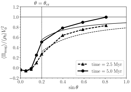
Figure 15: Dependence of $\langle\Pi_{\mathrm{mag}}\rangle$ on $\sin\theta$. The solid and dashed lines correspond to the magnetic stresses measured at $t=2.5$ Myr and $5.0$ Myr, respectively. The vertical axis is normalized by the upstream ram pressure. The dotted vertical line represents the critical angle.

The behavior of $\langle\Pi_{\mathrm{mag}}\rangle$ is determined by whether $\theta$ is larger than $\theta_{\mathrm{cr}}$ or not. If $\theta<\theta_{\mathrm{cr}}$, $\langle\Pi_{\mathrm{mag}}\rangle$ is almost independent of time and remains almost zero. For $\theta>\theta_{\mathrm{cr}}$, $\langle\Pi_{\mathrm{mag}}\rangle$ approaches $\langle\rho_{0}\rangle V_{0}^{2}$ as turbulence decays. The magnetic stresses for larger $\theta$ models reach $\langle\rho_{0}\rangle V_{0}^{2}$ earlier as shown in Fig. 14. At each epoch, the analytic estimate of the magnetic stress is plotted as the thin line. It is confirmed that the predictions from the analytic model are consistent with the simulation results, although there are some discrepancies. The analytic model slightly underestimates the magnetic stress for larger $\theta$ because of the weak negative dependence of $\delta v_{x}$ on $\theta$ found in Figs. 5a and 6.

We should note that, strictly speaking, $\langle\Pi_{\mathrm{mag}}\rangle$ remains almost zero not for $\theta<\theta_{\mathrm{cr}}$ but for $\theta<0.6\theta_{\mathrm{cr}}~{}(\sin\theta<0.12)$ in Fig. 15. A model with $\theta\leq 0.6\theta_{\mathrm{cr}}$ does not show a decrease in $\langle P_{\mathrm{ram}}\rangle$. For $\theta\geq\theta_{\mathrm{cr}}$, the shock-amplified magnetic field controls the post-shock dynamics and $\delta v_{x}$ decreases, obeying $\delta v_{x}\sim\delta v_{x0}(t/t_{0})^{-1/2}$. The angle range of $0.6\theta_{\mathrm{cr}}<\theta<\theta_{\mathrm{cr}}$ exhibits the transition between the layers regulated by ram pressure ($\langle\Pi_{\mathrm{mag}}\rangle\sim 0,~{}\langle P_{\mathrm{ram}}\rangle\sim\langle\rho_{0}\rangle V_{0}^{2}$) and those regulated by magnetic stress ($\delta v_{x}\sim\delta v_{x0}(t/t_{0})^{-1/2}$). Although the importance of $\langle\Pi_{\mathrm{mag}}\rangle$ increases with time in the total momentum flux, the ram pressure disturbs the post-shock layer significantly, leading to a slower decrease in $\delta v_{x}$ ($\delta v_{x}>\delta v_{x0}(t/t_{0})^{-1/2}$).

4.2.2 Mean Post-shock Densities

Fig. 16 shows $\langle n_{\mathrm{sh}}\rangle$ measured at three different epochs as a function of $\sin\theta$. The dashed line corresponds to $\langle n_{\mathrm{sh}}\rangle_{\mathrm{m}}$ as a function of $\sin\theta$ (Equation (23)). At a fixed $\theta$ the mean post-shock density approaches $\langle\rho_{\mathrm{sh}}\rangle_{\mathrm{m}}$ as $\delta v_{x}$ decreases, because the difference between $\langle n_{\mathrm{sh}}\rangle$ and $\langle n_{\mathrm{sh}}\rangle_{\mathrm{m}}$ indicates the significance of the ram pressure. The analytic estimates shown in Equation (23) at the three different epochs are plotted by the three thin lines. The mean post-shock densities predicted from Equation (23) are consistent with those derived from the simulation results at each epoch for $\theta\geq\theta_{\mathrm{cr}}$.

Note that the angle ($\theta\sim\theta_{\mathrm{cr}}$) that gives the maximum $\langle n_{\mathrm{sh}}\rangle$ does not depend on time, although $\langle n_{\mathrm{sh}}\rangle$ for larger $\theta$ reaches $\langle n_{\mathrm{sh}}\rangle_{\mathrm{m}}$ earlier. This is because $\langle n_{\mathrm{sh}}\rangle_{\mathrm{m}}\propto(\sin\theta)^{-1}$ is a decreasing function of $\theta$.

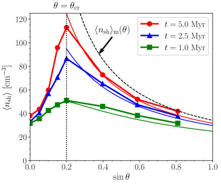
Figure 16: The mean post-shock densities at the three different epochs $t=5~{}$Myr (red), $t=2.5$ Myr (blue), and $t=1$ Myr (green) are plotted as a function of $\sin\theta$. At each epoch, the analytic estimation of $\langle n_{\mathrm{sh}}\rangle$ (Equation (23)) is plotted as the thin line with the same color. The dashed line indicates $\langle n_{\mathrm{sh}}\rangle_{\mathrm{sh}}$ given by Equation (25). The dotted vertical line represents the critical angle.

Although the magnetic stress starts to show a considerable growth at $\theta=0.6\theta_{\mathrm{cr}}$ in Fig. 15, $\langle n_{\mathrm{sh}}\rangle$ appears to increase smoothly for $\theta<\theta_{\mathrm{cr}}$ in Fig. 16. The smooth increase of $\langle n_{\mathrm{sh}}\rangle$ for $\theta\leq 0.6\theta_{\mathrm{cr}}$ is explained as follows. For $\theta\leq 0.6\theta_{\mathrm{cr}}$, $\delta v_{x}$ gradually decreases with $\theta$ (Fig. 6) although $\langle P_{\mathrm{ram}}\rangle\sim\langle\rho_{0}\rangle V_{0}^{2}$ is constant. From the relation $\langle P_{\mathrm{ram}}\rangle\propto\langle n_{\mathrm{sh}}\rangle\delta v_{x}^{2}$, $\langle n_{\mathrm{sh}}\rangle$ should increase with $\theta$ as shown in Fig. 16. Although $\langle n_{\mathrm{sh}}\rangle$ increases smoothly with $\theta$ for $\theta<\theta_{\mathrm{cr}}$, its manner of the time evolution of $\langle n_{\mathrm{sh}}\rangle$ suddenly changes at an angle near $\theta=0.6\theta_{\mathrm{cr}}$. Fig. 16 clearly shows that $\langle n_{\mathrm{sh}}\rangle$ increases with time for $\sin\theta=0.15~{}(\theta=0.75\theta_{\mathrm{cr}})$ while $\langle n_{\mathrm{sh}}\rangle$ does not increase significantly and is saturated around $60~{}\mathrm{cm}^{-3}$ for $\sin\theta=0.1~{}(\theta=0.5\theta_{\mathrm{cr}})$.

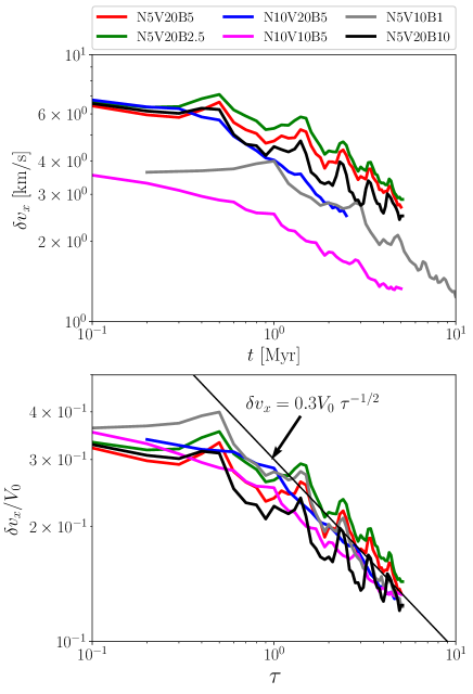
Figure 17: Top panel: time evolution of the longitudinal velocity dispersions for various models. The velocity dispersions are measured for N5V20B5 ($\theta=11^{\circ}$), N10V20B5 ($\theta=23^{\circ}$), N5V10B1 ($\theta=36^{\circ}$), N5V20B2.5 ($\theta=23^{\circ}$), N10V10B5 ($\theta=11^{\circ}$), and N5V20B10 ($\theta=11^{\circ}$). The bottom panel is the same as the top panel but the horizontal axis is changed to $\tau=t~{}(\langle n_{0}\rangle/5~{}\mathrm{cm}^{-3})(V_{0}/20~{}\mathrm{km~{}s^{-1}})/(1~{}\mathrm{Myr})$ and the vertical axis is normalized by $V_{0}$.

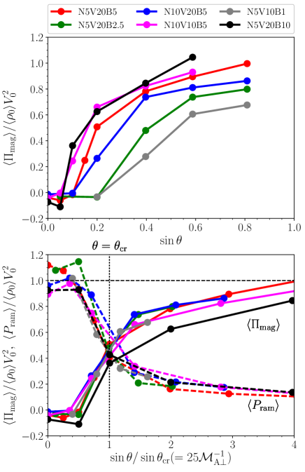
Figure 18: Top panel: mean magnetic stresses in the post-shock layers for various parameter sets of $(\langle n_{0}\rangle,V_{0},B_{0})$, which are tabulated in Table 1, as a function of $\sin\theta$. The magnetic stresses are measured at $\tau=5$. The bottom panel is the same as the top panel but the horizontal axis is normalized by the critical value ($\sin\theta_{\mathrm{crit}}$) shown in Equation (28). For each model, the mean ram pressures in the post-shock layer are also plotted as the dashed line with the same color. The vertical dotted line represents the $\theta=\theta_{\mathrm{cr}}$ line.

5 Parameter Survey

In Section 3, we presented the results for the fiducial parameter set ($\langle n_{0}\rangle=5~{}\mathrm{cm}^{-3}$, $B_{0}=5~{}\mu\mathrm{G}$, $V_{0}=20~{}\mathrm{km~{}s^{-1}}$). In this section, a parameter survey is performed by changing $(\langle n_{0}\rangle,V_{0},B_{0})$. The adopted parameters are summarized in Table 1. To save computational costs, we conducted the parameter survey with half the resolution, $512\times 256\times 256$, compared to the fiducial parameter set shown in Section 3. We have checked that at least the global quantities, $\langle P_{\mathrm{ram}}\rangle$ and $\langle\Pi_{\mathrm{mag}}\rangle$, are consistent with those with twice the resolution (the fractional differences are as small as $10\%$ in the fiducial parameter set). In each of the models, the simulations are performed by changing $\theta$, and $\langle P_{\mathrm{ram}}\rangle$ and $\langle\Pi_{\mathrm{mag}}\rangle$ are calculated as functions of $\theta$.

The top panel of Fig. 17 shows the time evolution of $\delta v_{x}$ for various models. For each model, we measure $\delta v_{x}$ at an angle $\theta$ where $\langle\Pi_{\mathrm{mag}}\rangle$ increases with time. The longitudinal velocity dispersions for all the models decrease with time in a similar manner (Fig. 5a). The bottom panel of Fig. 17 shows that $\delta v_{x}$ roughly follows a universal law,

$$\delta v_{x}=0.3V_{0}\tau^{-1/2}.$$ (27)

where $\tau=t\times(\langle n_{0}\rangle/5~{}\mathrm{cm}^{-3})\left(V_{0}/20~{}\mathrm{km~{}s^{-1}}\right)/(1~{}\mathrm{Myr})$. Equation (27) is reduced to Equation (13) in the fiducial model. Interestingly, the time evolution of $\delta v_{x}/V_{0}$ does not depend on the field strength sensitively, and it is characterized only by the accumulated mean column density $\sigma=2\langle\rho_{0}\rangle V_{0}t$, which is proportional to $\tau$. We compare these results for the models at $\tau=5$ when the mean visual extinction reaches 1.6.

Model name	$\langle n_{0}\rangle$ [cm-3]	$V_{0}$ [km s-1]	$B_{0}$ [$\mu$G]	$\displaystyle{\cal M}_{\mathrm{A}}$
N5V20B5	5	20	5	4.9
N5V20B2.5	5	20	2.5	9.7
N5V10B1	5	10	1	12
N10V20B5	10	20	5	6.9
N10V10B5	10	10	5	3.4
N5V20B10	5	20	10	2.4

Table 1: Model parameters. The last column indicates the Alfvén Mach number ${\cal M}_{\mathrm{A}}=V_{0}\sqrt{4\pi\langle\rho_{0}\rangle}/B_{0}$

The top panel of Fig. 18 shows $\langle\Pi_{\mathrm{mag}}\rangle$ as a function of $\sin\theta$ for various parameter sets. For a given parameter set $(\langle n_{0}\rangle,V_{0},B_{0})$, the $\theta$-dependence of $\langle\Pi_{\mathrm{mag}}\rangle$ is similar to that for the fiducial parameter set as shown in Fig. 15. The averaged magnetic stress $\langle\Pi_{\mathrm{mag}}\rangle$ increases monotonically with $\theta$. The only difference is the values of the critical angles below which $\langle\Pi_{\mathrm{mag}}\rangle$ is almost zero.

Here, we present an analytic estimate of the critical angle that can explain the results in different parameter sets ($\langle n_{0}\rangle$, $V_{0}$, $B_{0}$) using the analytic model developed in Section 4. We found that $\delta v_{x}$ is roughly proportional to $V_{0}$ at least in the $V_{0}$ range $10~{}\mathrm{km~{}s^{-1}}\leq V_{0}\leq 20~{}\mathrm{km~{}s^{-1}}$ for large angles from Fig. 17. At the critical angle, $\delta v_{x,\mathrm{eq}}(\theta_{\mathrm{cr}})$ is equal to $0.15V_{0}$ in the fiducial parameter set (Fig. 14). If this is the case also for other parameter sets, one obtains

$$\sin\theta_{\mathrm{cr}}=0.2\left(\frac{\langle n_{0}\rangle}{5~{}\mathrm{cm}^{-3}}\right)^{1/2}\left(\frac{V_{0}}{20~{}\mathrm{km~{}s^{-1}}}\right)\left(\frac{B_{0}}{5~{}\mu\mathrm{G}}\right)^{-1}.$$ (28)

Equation (28) is rewritten as

$${\cal M}_{\mathrm{A\perp,cr}}=\frac{V_{0}}{C_{\mathrm{A0\perp}}(\theta_{\mathrm{cr}})}=25,$$ (29)

meaning that if the Alfvén Mach number with respect to the perpendicular field component, ${\cal M}_{\mathrm{A\perp}}=V_{0}/C_{\mathrm{A0\perp}}$, is larger than 25, the super-Alfvénic velocity dispersion is maintained.

Let us derive the critical angle (Equation (28)) from the following simple argument. In the early phase, the velocity dispersion parallel to the $x$-axis takes a roughly constant value of

$$\delta v_{x}\sim\sqrt{\epsilon}V_{0},$$ (30)

where Equation (12) is used. If the magnetic stress mainly supports the post-shock layer against the upstream ram pressure, the post-shock Alfvén speed $C_{\mathrm{A,sh}}$ becomes

$$C_{\mathrm{A,sh}}=\left(\frac{V_{0}B\sin\theta}{\sqrt{2\pi\langle\rho_{0}\rangle}}\right)^{1/2},$$ (31)

where we use Equation (25) and $B_{\mathrm{sh,\perp}}^{2}/8\pi=\langle\rho_{0}\rangle V_{0}^{2}$. If $\delta v_{x}<C_{\mathrm{A,sh}}$, the magnetic field cannot be bent by the velocity dispersion parallel to the $x$-axis. From Equations (30) and (31), the critical angle $\theta_{\mathrm{cr}}^{\prime}$ satisfying $\delta v_{x}\sim C_{\mathrm{A,sh}}$ is given by

$$\sin\theta_{\mathrm{cr}}^{\prime}\sim 0.3\left(\frac{\epsilon}{0.1}\right)\left(\frac{\langle n_{0}\rangle}{5~{}\mathrm{cm}^{-3}}\right)^{1/2}\left(\frac{V_{0}}{20~{}\mathrm{km~{}s^{-1}}}\right)\left(\frac{B_{0}}{5~{}\mu\mathrm{G}}\right)^{-1}.$$ (32)

The parameter dependence of $\sin\theta_{\mathrm{cr}}^{\prime}$ is consistent with that of $\sin\theta_{\mathrm{cr}}$ although $\sin\theta_{\mathrm{cr}}^{\prime}$ is slightly larger than $\sin\theta_{\mathrm{cr}}$.

The bottom panel of Fig. 18 clearly shows that each of $\langle\Pi_{\mathrm{mag}}\rangle/\langle\rho_{0}\rangle V_{0}^{2}$ and $\langle P_{\mathrm{ram}}\rangle/\langle\rho_{0}\rangle V_{0}^{2}$ for all the models follows a universal line if $\sin\theta/\sin\theta_{\mathrm{cr}}$ is used as the horizontal axis. The ratio $\sin\theta/\sin\theta_{\mathrm{cr}}$ can be expressed as $25{\cal M}_{\mathrm{A\perp}}^{-1}$. The reason why both $\langle\Pi_{\mathrm{mag}}\rangle/\langle\rho_{0}\rangle V_{0}^{2}$ and $\langle P_{\mathrm{ram}}\rangle/\langle\rho_{0}\rangle V_{0}^{2}$ depend only on ${\cal M}_{\mathrm{A\perp}}$ is that all the models have almost the same $\delta v_{x}/V_{0}\sim 0.13$ at $\tau=5$ (Fig. 17). From Equation (23), one finds that $\langle\rho_{\mathrm{sh}}\rangle/\langle\rho_{0}\rangle$ depends only on ${\cal M}_{\mathrm{A\perp}}$ if $\delta v_{x}/V_{0}$ is fixed at 0.13. Substituting Equation (23) with $\delta v_{x}/V_{0}=0.13$ into Equations (21) and (22), it is found that $\langle\Pi_{\mathrm{mag}}\rangle/\langle\rho_{0}\rangle V_{0}^{2}$ and $\langle P_{\mathrm{ram}}\rangle/\langle\rho_{0}\rangle V_{0}^{2}$ are determined only by ${\cal M}_{\mathrm{A\perp}}$ as in $\langle\rho_{\mathrm{sh}}\rangle/\langle\rho_{0}\rangle$.

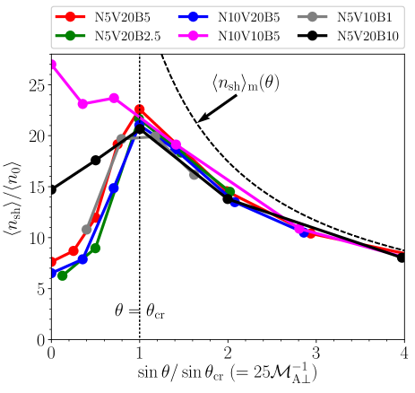
Figure 19: Mean post-shock densities for various parameter sets of $(\langle n_{0}\rangle,V_{0},B_{0})$, which are summarized in Table 1, as a function of $\sin\theta$. The post-shock densities are measured at $t=5~{}\mathrm{Myr}~{}(\langle n_{0}\rangle/5~{}\mathrm{cm}^{-3})^{-1}\left(V_{0}/20~{}\mathrm{km~{}s^{-1}}\right)^{-1}$. The vertical axis is normalized by the upstream mean density and the horizontal axis is normalized by the critical value ($\sin\theta_{\mathrm{crit}}$) shown in Equation (28). The dashed line corresponds to $\langle n_{\mathrm{sh}}\rangle_{\mathrm{m}}$ shown in Equation (25). The vertical dotted line shows $\theta=\theta_{\mathrm{cr}}$.

The mean post-shock densities normalized by $\langle n_{0}\rangle$ for various models are plotted as a function of $\sin\theta/\sin\theta_{\mathrm{cr}}$ in Fig. 19. The dashed line corresponds to $\langle n_{\mathrm{sh}}\rangle_{\mathrm{m}}$, which is rewritten as $\langle n_{\mathrm{sh}}\rangle_{\mathrm{m}}/\langle n_{0}\rangle=35~{}(\sin\theta/\sin\theta_{\mathrm{cr}})^{-1}$. For angles larger than $\sim\theta_{\mathrm{cr}}$, $\langle n_{\mathrm{sh}}\rangle/\langle n_{0}\rangle$ in all the models is approximated by an universal line as a function of $\sin\theta/\sin\theta_{\mathrm{cr}}$ (Fig. 19). By contrast, the behavior of $\langle n_{\mathrm{sh}}\rangle/\langle n_{0}\rangle$ for angles smaller than $\sim\theta_{\mathrm{cr}}$ can be divided into two groups. One group contains models N10V20B5, N5V10B1, and N5V20B2.5, where $\langle n_{\mathrm{sh}}\rangle$ rapidly decreases with decreasing $\theta$ from $\theta\sim\theta_{\mathrm{cr}}$ in a manner similar to that for the fiducial parameter set (N5V20B5). This group is referred to as the low-$\langle n_{\mathrm{sh}}\rangle$ group. All the lines of this group converge to a universal line in the ($\sin\theta/\sin\theta_{\mathrm{cr}}$, $\langle n_{\mathrm{sh}}\rangle/\langle n_{0}\rangle$) plane. However, models N10V10B5 and N5V20B10 do not show a rapid decrease in $\langle n_{\mathrm{sh}}\rangle$ as $\theta$ decreases. Especially for model N10V10B5, the post-shock layers are dense even for $\theta<\theta_{\mathrm{cr}}$, and a sharp $\langle n_{\mathrm{sh}}\rangle$ peak disappears.

The density enhancement for $\theta<\theta_{\mathrm{cr}}$ in model N10V10B5 arises from the fact that $\delta v_{x}$ gradually decreases with time. In the low-$\langle n_{\mathrm{sh}}\rangle$ group including the fiducial model, $\delta v_{x}$ is found not to decrease for $\theta<\theta_{\mathrm{cr}}$ because the CNM clumps are not decelerated significantly after passing through the shock fronts. We speculate that the difference between the $\delta v_{x}$ evolutions for model N10V10B5 and the low-$\langle n_{\mathrm{sh}}\rangle$ group comes from the following three points. First, because ${\cal M}_{\mathrm{A}}$ is lower for model N10V10B5 than for the low-$\langle n_{\mathrm{sh}}\rangle$ group where ${\cal M}_{\mathrm{A}}\gtrsim 5$ (Table 1), the magnetic field is expected to work more effectively than in the low-$\langle n_{\mathrm{sh}}\rangle$ group. Indeed, at $\tau=5$, $\langle\Pi_{\mathrm{mag}}\rangle/\langle\rho_{0}\rangle V_{0}^{2}$ for model N10V10B5 is 2.5 times larger than that for the fiducial model. However, lower Alfvén Mach numbers are not a sufficient condition to get larger $\langle n_{\mathrm{sh}}\rangle/\langle n_{0}\rangle$ because $\langle n_{\mathrm{sh}}\rangle/\langle n_{0}\rangle$ is larger for model N10V10B5 than for model N5V20B5 although ${\cal M}_{\mathrm{A}}$ is lower for model N5V20B5. Thus, the other points appear to be required. The second point is that the collision speed for model N10V10B5 is lower than in the fiducial model, indicating that the upstream CNM clumps have lower momenta, which allow them to be decelerated more easily. The third point is the larger upstream mean density for model N10V10B5, which enhances the volume filling factor of the CNM phase. A collision between CNM clumps is more probable than one between a CNM clump and WNM.

We should note that even for models N10V10B5 and N5V20B10 the super-Alfvénic turbulence is maintained without decay because $\langle P_{\mathrm{ram}}\rangle$ is much larger than $\langle\Pi_{\mathrm{mag}}\rangle$ as shown in Fig. 18. The decrease in $\delta v_{x}$ does not lead to an increase in $\langle\Pi_{\mathrm{mag}}\rangle$. This contrasts with the case with $\theta>\theta_{\mathrm{cr}}$, in which $\langle\Pi_{\mathrm{mag}}\rangle$ increases with decreasing $\delta v_{x}$. For $\theta<\theta_{\mathrm{cr}}$, the decrease in $\delta v_{x}$ is compensated by the increase in the mean post-shock density to maintain pressure balance between $\langle P_{\mathrm{ram}}\rangle$ and the upstream ram pressure.

6 Discussion

6.1 Sub-Alfvénic Colliding Flows

The parameter survey in Section 5 shows that the global time evolution of the post-shock layers is described by the analytic model. It should be noted that the simulation results depend not on the parallel field component ($B_{0}\cos\theta$) but only on the perpendicular field component ($B_{0}\sin\theta$). This is simply because super-Alfvénic colliding flows are considered in this paper. The parallel field component does not play an important role.

The analytic model thus cannot be applied for all parameter sets of ($\langle n_{0}\rangle,V_{0},B_{0}$). If a colliding flow is sub-Alfvénic, the magnetic field is too strong to be bent by shock compression. Instead, the gas is allowed to accumulate along the magnetic field through slow shocks. From the MHD Rankine-Hugoniot relations, Inoue & Inutsuka (2009) derived a criterion required to form slow shocks as follows:

$$B_{0}>B_{\mathrm{cr}}\equiv\frac{2}{3}V_{0}\sqrt{4\pi\rho_{0}},$$ (33)

where $\rho_{0}$ is the uniform upstream density and the ratio of specific heats is set to $5/3$. We should note that equation (33) is different from equation (14) in Inoue & Inutsuka (2009), where the left-hand side of equation (33), $B_{0}$, is replaced by $B_{0}\cos\theta$. Equation (33) corresponds to a necessary condition to form slow shocks. If equation (33) is not satisfied, slow shocks are not generated for any angle. Equation (33) is roughly the same as the condition of sub-Alfvénic colliding flows, which is given by $B_{0}>V_{0}\sqrt{4\pi\rho_{0}}$.

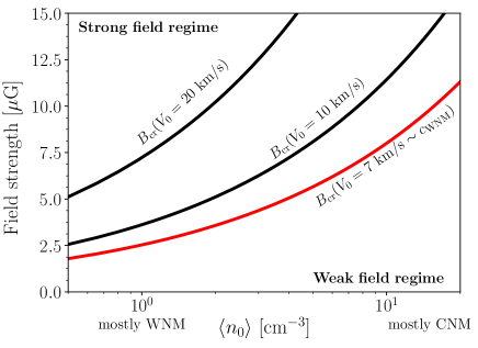
Figure 20: Density dependence of $B_{\mathrm{cr}}$ for three different collision speeds. At each collision speed, the region above (below) the line $B=B_{\mathrm{cr}}$ belongs to the strong (weak) field regime.

Fig. 20 shows $B_{\mathrm{cr}}$ as a function of $\langle n_{0}\rangle$ for three different collision speeds. In the figure, for a given $V_{0}$, the region above (below) the line $B=B_{\mathrm{cr}}$ is referred to as the strong (weak) field regime. The range of $B_{0}$ that belongs to the weak field regime is wider for higher mean densities because Alfvén speed is a decreasing function of gas density. Shock compression of denser atomic gases is likely to be in the weak field regime, where the analytic model can be applied. Since this paper focuses on the MC formation from dense atomic gases that have already been piled up by previous episodes of compression, all our simulations are in the weak field regime.

6.2 Comparison with Previous Studies

Most simulations of WNM colliding flow have been done in the cases where the collision direction is parallel to the mean magnetic field (Hennebelle et al., 2008; Banerjee et al., 2009; Vázquez-Semadeni et al., 2011; Körtgen & Banerjee, 2015; Zamora-Avilés et al., 2018). One of the differences between two-phase and WNM colliding flows is that the two-phase colliding flows are highly inhomogeneous. Our results showed that the inhomogeneity of colliding flows enhances longitudinal velocity dispersion for $\theta\sim 0^{\circ}$ (also see Inoue & Inutsuka, 2012; Carroll-Nellenback et al., 2014; Forgan & Bonnell, 2018). We also found density enhancement for $\theta\sim 0^{\circ}$ in the models where the field strength is relatively large and the Alfvén Mach number of the colliding flow is close to unity in Fig. 16. This is consistent with the results of Heitsch et al. (2009) and Zamora-Avilés et al. (2018) who found that the post-shock layers become denser for stronger magnetic fields with a fixed collision speed (also see Heitsch et al., 2007, for isothermal colliding flows).

In the two-phase colliding flows, the pre-existing upstream CNM clumps become an ingredient of the post-shock CNM clumps. For WNM colliding flows with oblique fields, Inoue & Inutsuka (2009) showed that only HI clouds with a density of $\sim 10$ cm^-3 form. Heitsch et al. (2009) also reported that the formation of dense clouds is prohibited in a WNM colliding flow with a perpendicular magnetic field. Our results, however, show that a large amount of the dense gas with $>10^{2}~{}\mathrm{cm}^{-3}$ exists in the post-shock layers even for model $\Theta 36$ (Fig. 10). This is simply because the dense gases with $>10^{2}~{}\mathrm{cm}^{-3}$ can be directly supplied by the accretion of the pre-existing CNM clumps, whose densities are enhanced over $10^{2}~{}\mathrm{cm}^{-3}$ by the super-Alfvénic shock compression. Note that the CNM mass fraction in the post-shock layer is larger than the upstream CNM mass fraction of $\sim 0.5$. This indicates that the dense gases with $>10^{2}~{}\mathrm{cm}^{-3}$ are also provided from the surrounding diffuse gas through the thermal instability.

6.3 Implications for the Formation of MCs

We found that the CO molecules form efficiently around $\theta\sim\theta_{\mathrm{cr}}$ where the dense gas with $>10^{3}~{}\mathrm{cm}^{-3}$ is efficiently generated (Fig. 10). For $\theta<\theta_{\mathrm{cr}}$ ($\theta>\theta_{\mathrm{cr}}$), the large anisotropic velocity dispersion (the magnetic stress) prevents the gas from being dense enough to form CO molecules (Figs. 10 and 11). Although the simulations are terminated in the early phase, the mass fraction of CO-forming gases exceeds 17% for $\theta\sim\theta_{\mathrm{cr}}$. The CO fraction will continue to increase if we follow further evolution of the post-shock layers.

The setup of head-on colliding flows of the atomic gas leads to somewhat artificial results, especially for $\theta<\theta_{\mathrm{cr}}$ in the models belonging to the low-$\langle n_{\mathrm{sh}}\rangle$ group, or model $\Theta 3$ for the fiducial model. The lower post-shock mean density and faster shock propagation velocity for model $\Theta 3$ can be explained as follows: the upstream CNM clumps that are not decelerated at the shock due to high density continue to stream roughly along the $x$-axis and finally hit/push the shock wave on the opposite side. We think that this effect can be expected only for a very limited astronomical situation where two identical flows collide as in the present simulations. If we consider, for instance, the growth of an MC through an interaction with a shocked HI shell created by a supernova shock or an expanding HII region (e.g. Inutsuka et al., 2015), the interaction would not destroy the MC even if the HI shell accretes to the MC along the magnetic field. This is because the MC would have a mass (or column density) enough to decelerate the accreting HI gas. In addition to this, when we consider the effect of gravity, we can expect that the expansion of the shocked region for model $\Theta 3$ is stopped around $t\gtrsim 5$ Myr (see equation C1), because the freely flying CNM clumps leaving the shocked region are decelerated by the gravity (Appendix C). In the previous simulation done by Inoue & Inutsuka (2012), they prevented the free propagation of CNM that crosses the $x$-boundary planes by setting a viscosity at the boundaries to mimic the effect of gravity. They found that even for the condition $\theta=0^{\circ}$, a realistic MC can be formed at $t\sim 7$ Myr. Self-gravity also contributes to local gas compression. This will further promote the formation of MCs. By contrast, if $\theta$ is sufficiently large, the formation of MCs is expected to remain inefficient even if the self-gravity becomes important because density enhancement is suppressed by the magnetic pressure.

Our results show that the physical properties of cold clouds depend strongly on the field orientation especially around $\theta\sim\theta_{\mathrm{cr}}$. To estimate how rare a shock compression with $\theta<\theta_{\mathrm{cr}}$ is, the contours of the critical angles in the ($\langle n_{0}\rangle,B_{0}$) plane for two different collision speeds are plotted in Fig. 21. The gray regions in Fig. 21 are not focused on in this paper (Section 6.1).

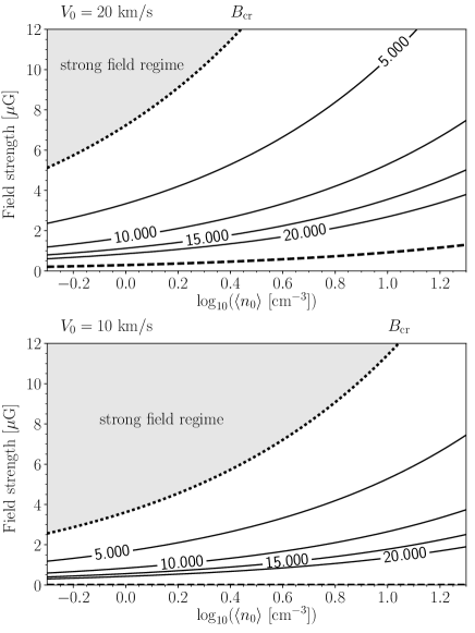
Figure 21: Contours of the critical angles in the ($\langle n_{0}\rangle$, $B_{0}$) plane for $V_{0}=20~{}$km s^-1 (top) and $V_{0}=10~{}$km s^-1 (bottom). The numbers on the contours indicate the corresponding angles in degrees. In each panel, the dotted line corresponds to the critical field strength shown in equation (33). In the regions below the dashed lines, the critical angles become $90^{\circ}$, indicating that turbulence does not decay for any angle because of the low field strength.

Fig. 21 shows that the critical angles are very small unless magnetic fields are weak ($B_{0}<1~{}\mu$G). To estimate the probability of realizing a shock compression with $\theta\leq\theta_{\mathrm{cr}}$ ($P(\theta\leq\theta_{\mathrm{cr}})$), it is assumed that a shock compression occurs isotropically in a uniform magnetic field. The probability is proportional to the solid angle $\Omega$ of a cone with apex angle $2\theta_{\mathrm{cr}}$ ($\Omega=4\pi\sin^{2}(\theta_{\mathrm{cr}}/2)$). Using $\Omega$, the probability is given by $P(\theta\leq\theta_{\mathrm{cr}})=2\times\Omega/4\pi=2\sin^{2}(\theta_{\mathrm{cr}}/2)$, where the factor of two is to account for the cases of $\theta\leq\theta_{\mathrm{cr}}$ and $\theta\geq\pi-\theta_{\mathrm{cr}}$. Finally, we obtain $P(\theta\leq\theta_{\mathrm{cr}})\simeq\theta_{\mathrm{cr}}^{2}/2$ because the critical angle is small for $B_{0}>1~{}\mu$G (Fig. 21) (also see Inutsuka et al., 2015). The probability $P(\theta\leq\theta_{\mathrm{cr}})=0.017~{}(\theta_{\mathrm{cr}}/11^{\circ})^{2}$ is extremely low in the fiducial parameter set. From Fig. 11, shock compression with larger $\theta$ significantly suppresses the formation of dense gases and CO. At least in the early evolution of MCs, the shock compression with angles less than $\xi\theta_{\mathrm{cr}}$ ($\xi=1-2$) is expected to contribute to an efficient MC formation because $f_{>10^{3}}$ and $f_{\mathrm{CO}}$ decreases rapidly with $\theta$ for $\theta>\theta_{\mathrm{cr}}$ (Figs. 10 and 11). The probability of realizing the compression with $\theta<\xi\theta_{\mathrm{cr}}$ is $P(\theta<\xi\theta_{\mathrm{cr}})=2\pi\xi^{2}\theta_{\mathrm{cr}}^{2}/4\pi\sim 0.04~{}(\xi/1.5)^{2}(\theta_{\mathrm{cr}}/11^{\circ})^{2}$.

The free parameter $\xi$ cannot be determined from our work because we focused on the early stage of the MC formation. We expect that $\xi$ is determined as a function of ($\langle n_{0}\rangle$, $V_{0}$, $B_{0}$) by whether cold clouds become massive enough for star formation to occur against the magnetic pressure. We will present the results of long-term simulations including gravity in a future paper.

6.4 Caveats

Although the simple setup of steady head-on colliding flows enables us to investigate the detailed post-shock dynamics, we ignore several aspects of physics that are important in the galactic environment.

6.4.1 Head-on Collision

We consider that colliding flows are generated by adjacent expanding super-bubbles and galactic spiral waves. However, head-on collisions considered in this paper are an extreme case. In realistic situations, we need to take into account an offset colliding flow, which would induce a global shear motion in the post-shock layer. The shear motion can affect the post-shock dynamics significantly (Fogerty et al., 2016).

Colliding flows are not an optimal approximation in the cases of a single SN or multiple SNe, which are expected to contribute to the MC formation. They generate a hot bubble that drives an expanding shell confined by the shock front on the leading side and the contact discontinuity, which separates the shell from the hot bubble, on the trailing side. Especially for the almost parallel field models (for instance model $\Theta 3$), the existence of two shock fronts strongly affects the post-shock dynamics as discussed in Section 6.3. Kim & Ostriker (2015) investigated the evolution of shells expanding into realistic two-phase atomic gases. Because they ignore magnetic fields, their setups relate to the almost parallel field models in this work. In their simulations, pre-existing HI clouds strongly deform both the shock front and contact discontinuity, and the shells are widened. These behaviors are qualitatively consistent with our results. However, the effect of the contact discontinuity should affect the post-shock dynamics.

6.4.2 Local Simulations

Although the well-controlled setups of our local simulations allow us to perform a detailed analysis, the locality of our simulations is one of the caveats. In this paper, we consider a continuous supply of the atomic gas assuming constant values of $V_{0}$, $B_{0}$, and $\theta$.

First, we should note that shock compression has a finite duration in the galactic environment. We consider that colliding flows are generated by adjacent expanding super-bubbles and galactic spiral waves. Although our simulations are terminated earlier than the typical duration of super-bubbles and spiral waves (a few tens of megayears), it is worth discussing the time evolution of a post-shock layer after shock compression ceases. In local simulations, many studies took into account the finite duration of colliding flows (Vázquez-Semadeni et al., 2007; Banerjee et al., 2009; Vázquez-Semadeni et al., 2010, 2011; Körtgen & Banerjee, 2015; Zamora-Avilés et al., 2018). As the shock compression weakens, $B_{\mathrm{cr}}$ decreases with time in Fig. 20. Once $B_{\mathrm{cr}}$ becomes smaller than $B_{0}$, the magnetic field cannot be bent by the shock compression. Magnetic tension realigns the magnetic field with the upstream field direction. If the gravitational force is important, the gas accumulates along the realigned magnetic field.

Although all local simulations considered the MC formation via a single compression of the atomic gas, we need to consider multiple episodes of compressions to form giant MCs (Inutsuka et al., 2015; Kobayashi et al., 2017, 2018). Recent global simulations of galactic disks have also pointed out that global MCs experience collisional build-up driven by large-scale flows associated with the spiral arm and nearby supernova explosions during their growth and evolution (e.g., Dobbs et al., 2015; Baba et al., 2017). We will investigate the effect of multiple compressions during the MC formation in a local simulation to achieve high resolution in the future.

6.4.3 Limitation of the Analytic Model

The analytic model developed in Sections 4 and 5 describes the evolution of the averaged quantities $\langle n_{\mathrm{sh}}\rangle$, $\langle\Pi_{\mathrm{mag}}\rangle$, and $\langle P_{\mathrm{ram}}\rangle$ using the pressure balance across a post-shock layer. However, the post-shock dynamics is not fully understood because we do not explain why $\delta v_{x}$ obeys the universal law shown in equation (27) for $\theta>\theta_{\mathrm{cr}}$. It also remains an unsettled question what determines $\theta_{\mathrm{cr}}$ although $\theta_{\mathrm{cr}}^{\prime}$ is derived by the simple argument in Equation (32). We expect that the interaction between the upstream CNM clumps and the warm interclump gas is crucial in the post-shock dynamics. If $\theta$ is sufficiently small, the motion of CNM clumps triggers magnetic reconnection, which prevents the field lines from being compressed (Jones et al., 1996). The interaction between CNM clumps through magnetic field lines also plays an important role in the post-shock dynamics (Clifford & Elmegreen, 1983; Elmegreen, 1988). We will address these issues in forthcoming papers.

7 Summary

We investigated the early stage of the formation of MCs by colliding flows of the atomic gas, which has a realistic two-phase structure where HI clouds are embedded in warm diffuse gases. As parameters, we consider the mean density $\langle n_{0}\rangle$, the strength and direction of the magnetic field $B_{0}$, and the collision speed $V_{0}$ of the atomic gas.

First, we investigated the MC formation at a fiducial parameter set of $(\langle n_{0}\rangle=5~{}\mathrm{cm}^{-3},V_{0}=20~{}\mathrm{km~{}s^{-1}},B_{0}=5~{}\mu\mathrm{G})$ by changing the angle $\theta$ between the magnetic field and upstream flow. We focus on super-Alfvénic colliding flows $(V_{0}>B_{0}/\sqrt{4\pi\langle\rho_{0}\rangle})$ which are more likely for compression of denser atomic gases (Section 6.1). Our findings are as follows.

1. In the early phase, shock compression of the highly inhomogeneous atomic gas drives the velocity dispersions in the compression direction, which are as large as $\sim 0.3V_{0}$, regardless of $\theta$. The transverse velocity dispersions are much smaller than the longitudinal ones.

2. The later time evolution of the post-shock layers can be classified in terms of a critical angle $\theta_{\mathrm{cr}}$ which is roughly equal to $\sim 11^{\circ}$ for the fiducial parameter set.

3. If $\theta<\theta_{\mathrm{cr}}$, an upstream CNM clump is not decelerated when it passes through a shock front, and finally collides with the shock front on the opposite side. A highly super-Alfvénic velocity dispersion is maintained by accretion of the upstream CNM clumps. The velocity dispersion is highly biased in the compression direction. The magnetic field does not play an important role, and it is passively bent and stretched by the super-Alfvénic gas motion. The post-shock layer significantly expands in the compression direction as a result of the large velocity dispersion.

4. If $\theta>\theta_{\mathrm{cr}}$, the shock-amplified transverse magnetic field decelerates the CNM clumps moving in the compression direction. The decelerated CNM clumps are accumulated in the central region. The velocity dispersion in the compression direction decreases as $\propto t^{-1/2}$, and appears not to depend on $\theta$ sensitively. The time dependence may be explained if there is a mechanism that keeps the total kinetic energy in the compression direction constant. The velocity dispersion in the transverse direction does not decrease with time.

5. As a function of $\theta$, the mean post-shock densities have a sharp peak at an angle near $\theta\sim\theta_{\mathrm{cr}}$, regardless of time (Fig. 16). Around $\theta\sim\theta_{\mathrm{cr}}$, the gas compression occurs not only in the collision direction but also along the shock-amplified transverse magnetic field. As a result, the total mass of dense gases rapidly increases and CO molecules efficiently form even without self-gravity. The mean post-shock densities, the dense gas masses, and the CO abundances rapidly decrease toward $\theta<\theta_{\mathrm{cr}}$ ($\theta>\theta_{\mathrm{cr}}$) because of the ram pressure (magnetic stress).

6. By developing an analytic model and performing a parameter survey in the parameters of ($\langle n_{0}\rangle,V_{0},B_{0}$), we derive an analytic formula for the critical angle $\theta_{\mathrm{cr}}$ (Equation (28)), above which the shock-amplified magnetic field controls the post-shock dynamics. We also found that the mean ram and magnetic pressures in the post-shock layers evolve in a universal manner as a function of ${\cal M}_{\mathrm{A\perp}}$ and the accumulated column density for various parameter sets ($\langle n_{0}\rangle,V_{0},B_{0}$). The evolution of the mean post-shock densities also follows a universal law. However, in colliding flows with Alfvén Mach numbers less than $\sim 4$, lower collision speeds, and higher mean upstream densities, the post-shock mean densities can be high for $\theta<\theta_{\mathrm{cr}}$.

7. The critical angle $\theta_{\mathrm{cr}}$ takes a small value as long as magnetic fields are not very weak ($>1~{}\mu$G) (Fig. 21). If the atomic gas is compressed from various directions with respect to the field line direction, the compression with $\theta<\theta_{\mathrm{cr}}$ seems to be rare. Although we need further simulations including self-gravity, shock compression with angles a few times larger than the critical angle is expected not to contribute to an efficient MC formation because the CO formation is inefficient owing to the lack of dense gases.

Our results show that the post-shock structures depend strongly on $\theta$ in the case that $\theta$ is less than a few times $\theta_{\mathrm{cr}}$. This may create a diversity of the physical properties of dense clumps and cores in simulations including self-gravity. Self-gravity is also expected to affect the global structures of MCs. We will address the effect of self-gravity on the MC formation in forthcoming papers.

Appendix A The Effect of Radiative Cooling on the Evolution of CNM Clumps

The interaction of a shock wave with an isolated interstellar cloud for the adiabatic case was investigated by Klein et al. (1994). According to their estimation, the cloud is destroyed and mixed with the surrounding diffuse gas by the Kelvin-Helmholtz and Rayleigh-Taylor instabilities in several cloud-crushing times given by

$$t_{\mathrm{cc,CNM}}=\chi^{1/2}\frac{L_{\mathrm{CNM}}}{V_{0}}\sim 0.2~{}\mathrm{Myr}\left(\frac{\chi}{20}\right)^{1/2}\left(\frac{L_{\mathrm{CNM}}}{1~{}\mathrm{pc}}\right)\left(\frac{V_{0}}{20~{}\mathrm{km~{}s^{-1}}}\right)^{-1},$$ (A1)

where $\chi$ is the density contrast between the CNM and WNM, and $t_{\mathrm{cc,CNM}}$ is the timescale for the shock to travel the cloud size in the compression direction, $L_{\mathrm{CNM}}$. If there is turbulence in the post-shock region, the destruction timescale becomes even shorter (Pittard et al., 2009). Thus, shocked CNM clumps are expected to be destroyed quickly on a timescale less than 1 Myr.

For comparison, we perform another simulation without the cooling/heating processes for the $\theta=0^{\circ}$ case. The results are shown in Fig. 22. After passing through the shock fronts, the CNM clumps are quickly destroyed and are mixed up with the surrounding warm gases. The mixing causes the density distribution to be relatively smooth as shown in the top panel of Fig. 22. Unlike the results with radiative cooling, the velocity field in the post-shock layer appears not to be biased in the compression direction but to be randomized. This is consistent with the estimation in equation A1. The bottom panel of Fig. 22 shows local amplification of the magnetic field. This is formed by the Richtmyer-Meshkov instability, where the MHD interaction between a shock wave and a CNM clump develops vortices that amplify magnetic fields (Inoue et al., 2009; Sano et al., 2012).

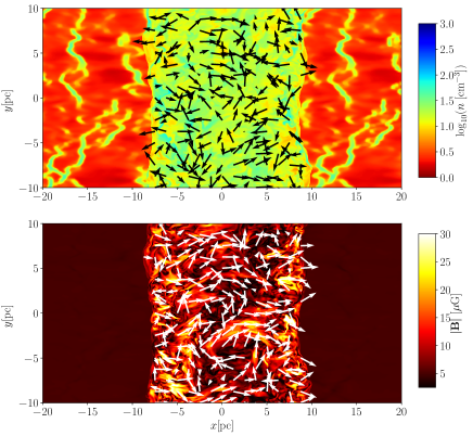
Figure 22: Maps of density (top panel) and field strength (bottom panel) in the $z=0$ plane at $t=1.2$ Myr for the adiabatic case where the cooling/heating processes are switched off in the same initial and boundary conditions. The arrows in the top and bottom panels indicate the directions of the velocity and magnetic fields, respectively.

Fig. 2, however, shows that the two-phase structure is clearly seen in the post-shock layers for all the models, indicating that the cooling/heating processes are important in the survival of the CNM clumps. This effect has been pointed out by Mellema et al. (2002), Melioli et al. (2005), and Cooper et al. (2009) in different contexts. The significance of the radiative processes is characterized by the cooling time given by $P/\left\{(\gamma-1)\Lambda\right\}$, where we use the following approximate cooling rate:

$$\Lambda\sim 3\times 10^{-28}n^{2}\sqrt{T}e^{-92/T}~{}\mathrm{erg~{}cm^{-3}~{}s^{-1}}$$ (A2)

(Koyama & Inutsuka, 2002). Just behind the shock front, the CNM temperature increases up to $3\mu m_{\mathrm{H}}V_{0}^{2}/16k_{\mathrm{B}}$ and the CNM density increases by a factor of 4 if the shock is adiabatic. The cooling time of the shocked CNM is estimated as

$$t_{\mathrm{cool,CNM}}\sim 1.2\times 10^{-2}~{}\mathrm{Myr}\left(\frac{V_{0}}{20~{}\mathrm{km~{}s^{-1}}}\right)\left(\frac{n_{\mathrm{CNM,sh}}}{200~{}\mathrm{cm}^{-3}}\right)^{-1},$$ (A3)

where $n_{\mathrm{CNM,sh}}$ is a typical CNM density in the post-shock region under the adiabatic assumption. Equations (A1) and (A3) indicate that the cooling time is much shorter than the cloud-crushing time. A shocked CNM clump quickly cools and condenses to reach a thermal equilibrium state. Although the CNM clumps fragment, this does not lead to complete mixing of the CNM clumps with the surrounding WNM. Instead, gas exchange owing to phase transition between CNM/WNM occurs (Iwasaki & Inutsuka, 2014; Valdivia et al., 2016). The large density contrast also contributes to the long lifetime of the CNM clumps (see Equation (A1)). Magnetic fields also increase the lifetime of the CNM clumps by reducing the growth rate of the Kelvin-Helmholtz instability.

Appendix B Evolution of the Hydrogen Molecule Fraction in a Post-shock Layer.

In this appendix, we estimate the H₂ fraction in a post-shock layer with a constant density of $n_{\mathrm{sh}}$. Since the fresh material, whose H₂ fraction is almost zero, is continuously supplied to the post-shock layer, the evolution of the H₂ fraction in the post-shock layer cannot be understood using a simple formation time of $(k_{\mathrm{H_{2}}}n_{\mathrm{sh}})^{-1}$, where $k_{\mathrm{H_{2}}}$ is the H₂ formation rate coefficient (Hollenbach & McKee, 1979).

Here we derive the H₂ fraction in the post-shock layer at an epoch of $t=t_{\mathrm{f}}$ as follows. The time evolution of the number density of atomic H is given by

$$\frac{dn_{\mathrm{H}}}{dt}=-2k_{\mathrm{H_{2}}}n_{\mathrm{sh}}n_{\mathrm{H}}.$$ (B1)

In order to derive an upper limit on the H₂ abundance, we neglect the photodissociation of H₂. The number of the hydrogen nuclei entering the post-shock layer from $t$ to $t+\Delta t$ is $2L_{0}^{2}V_{0}\langle n_{0}\rangle\Delta t$. Among them, the number of the hydrogen nuclei remaining in atomic H is given by

$$\Delta N_{\mathrm{H}}=2L_{0}^{2}V_{0}\langle n_{0}\rangle\Delta t\exp\left[-\int_{t}^{t_{\mathrm{f}}}2k_{\mathrm{H_{2}}}n_{\mathrm{sh}}dt\right],$$ (B2)

where we use the fact that most of the hydrogen nuclei are in atomic H just after the shock compression. By integrating Equation (B2) from $t=0$ to $t=t_{\mathrm{f}}$, one obtains the total number of atomic H at $t=t_{\mathrm{f}}$ as follows:

$$N_{\mathrm{H}}=2L_{0}^{2}V_{0}\langle n_{0}\rangle\int_{0}^{t_{\mathrm{f}}}\exp\left[-\int_{t}^{t_{\mathrm{f}}}2k_{\mathrm{H_{2}}}n_{\mathrm{sh}}ds\right]dt.$$ (B3)

If $n_{\mathrm{sh}}$ and $k_{\mathrm{H_{2}}}$ are constant with time, Equation (B2) is reduced to

$$N_{\mathrm{H}}=2L_{0}^{2}V_{0}\langle n_{0}\rangle\frac{1-e^{-2k_{\mathrm{H_{2}}}n_{\mathrm{sh}}t_{\mathrm{f}}}}{2k_{\mathrm{H_{2}}}n_{\mathrm{sh}}}.$$ (B4)

Finally, the H₂ fraction $f_{\mathrm{H2,ave}}$ is given by

$$f_{\mathrm{H2,ave}}\equiv\frac{N-N_{\mathrm{H}}}{N}=1-\frac{1-e^{-2k_{\mathrm{H_{2}}}n_{\mathrm{sh}}t_{\mathrm{f}}}}{2k_{\mathrm{H_{2}}}n_{\mathrm{sh}}t_{\mathrm{f}}},$$ (B5)

where $N=2L_{0}^{2}V_{0}\langle n_{0}\rangle t_{\mathrm{f}}$ is the total number of the hydrogen nuclei accumulated in the post-shock layer until $t=t_{\mathrm{f}}$.

Appendix C The Effect of Self-gravity in the Case that Magnetic Fields are Almost Parallel to Colliding Flows.

Here we estimate the timescale on which a freely propagating CNM clump leaving the shocked region is decelerated by the gravitational force from the shocked region. Let us consider a sheet with a surface density $\sigma$. If it is formed by the converging flows, we can write $\sigma=2\langle\rho_{0}\rangle V_{0}t$. Since the gravitational force exerted by the sheet on an object with mass $m$ from the sheet is given by $F_{\mathrm{G}}=2\pi mG\sigma$, the equation of motion for a cold clump that is freely flying outside of the sheet is given by $dv/dt=2\pi G\sigma$. Thus, a clump that is ejected from the sheet with a velocity $v_{\mathrm{ej}}$ is attracted by the self-gravitational force of the sheet and eventually pulled back at the time $t_{\mathrm{g}}\simeq\{v_{\mathrm{ej}}/(4\pi G\langle\rho_{0}\rangle V_{0})\}^{1/2}$. If we use typical parameters of the $\theta=3^{\circ}$ case, the timescale can be expressed as

$$t_{\mathrm{g}}\simeq 5~{}\mathrm{Myr}~{}\left(\frac{v_{\mathrm{ej}}}{5~{}\mathrm{km~{}s}^{-1}}\right)^{1/2}\left(\frac{\langle n_{0}\rangle}{5~{}\mathrm{cm}^{-3}}\right)^{-1/2}\left(\frac{V_{0}}{20~{}\mathrm{km~{}s^{-1}}}\right)^{-1/2}.$$ (C1)

This suggests that the shocked region would not expand after $t_{\mathrm{g}}\simeq 5$ Myr.

References

- Audit & Hennebelle (2005) Audit, E., & Hennebelle, P. 2005, A&A, 433, 1
- Audit & Hennebelle (2010) —. 2010, A&A, 511, A76
- Baba et al. (2017) Baba, J., Morokuma-Matsui, K., & Saitoh, T. R. 2017, MNRAS, 464, 246
- Balbus (1986) Balbus, S. A. 1986, ApJL, 303, L79
- Banerjee et al. (2009) Banerjee, R., Vázquez-Semadeni, E., Hennebelle, P., & Klessen, R. S. 2009, MNRAS, 398, 1082
- Beck (2001) Beck, R. 2001, Space Sci. Rev., 99, 243
- Blitz et al. (2007) Blitz, L., Fukui, Y., Kawamura, A., et al. 2007, 2007prpl conf, 81
- Blondin & Marks (1996) Blondin, J. M., & Marks, B. S. 1996, New A, 1, 235
- Bonnell et al. (2013) Bonnell, I. A., Dobbs, C. L., & Smith, R. J. 2013, MNRAS, 430, 1790
- Carroll-Nellenback et al. (2014) Carroll-Nellenback, J. J., Frank, A., & Heitsch, F. 2014, ApJ, 790, 37
- Chandrasekhar (1961) Chandrasekhar, S. 1961, Hydrodynamic and Hydromagnetic Stability (Oxford: Clarendon)
- Chevalier (1974) Chevalier, R. A. 1974, ApJ, 188, 501
- Choi & Stone (2012) Choi, E., & Stone, J. M. 2012, ApJ, 747, 86
- Clark et al. (2012) Clark, P. C., Glover, S. C. O., Klessen, R. S., & Bonnell, I. A. 2012, MNRAS, 424, 2599
- Clark et al. (2015) Clark, S. E., Hill, J. C., Peek, J. E. G., Putman, M. E., & Babler, B. L. 2015, PhPvL, 115, 241302
- Clifford & Elmegreen (1983) Clifford, P., & Elmegreen, B. G. 1983, MNRAS, 202, 629
- Cooper et al. (2009) Cooper, J. L., Bicknell, G. V., Sutherland, R. S., & Bland-Hawthorn, J. 2009, ApJ, 703, 330
- Crutcher et al. (2010) Crutcher, R. M., Wandelt, B., Heiles, C., Falgarone, E., & Troland, T. H. 2010, ApJ, 725, 466
- Dawson et al. (2011) Dawson, J. R., McClure-Griffiths, N. M., Kawamura, A., et al. 2011, ApJ, 728, 127
- Dawson et al. (2013) Dawson, J. R., McClure-Griffiths, N. M., Wong, T., et al. 2013, ApJ, 763, 56
- de Hoffmann & Teller (1950) de Hoffmann, F., & Teller, E. 1950, PhRv, 80, 692
- de Jong et al. (1980) de Jong, T., Boland, W., & Dalgarno, A. 1980, A&A, 91, 68
- Dobbs et al. (2012) Dobbs, C. L., Pringle, J. E., & Burkert, A. 2012, MNRAS, 425, 2157
- Dobbs et al. (2015) Dobbs, C. L., Pringle, J. E., & Duarte-Cabral, A. 2015, MNRAS, 446, 3608
- Draine (1978) Draine, B. T. 1978, ApJS, 36, 595
- Draine & Bertoldi (1996) Draine, B. T., & Bertoldi, F. 1996, ApJ, 468, 269
- Elmegreen (1988) Elmegreen, B. G. 1988, ApJ, 326, 616
- Evans & Hawley (1988) Evans, C. R., & Hawley, J. F. 1988, ApJ, 332, 659
- Field (1965) Field, G. B. 1965, ApJ, 142, 531
- Field et al. (1969) Field, G. B., Goldsmith, D. W., & Habing, H. J. 1969, ApJ, 155, L149
- Fogerty et al. (2016) Fogerty, E., Frank, A., Heitsch, F., et al. 2016, MNRAS, 460, 2110
- Folini et al. (2014) Folini, D., Walder, R., & Favre, J. M. 2014, A&A, 562, A112
- Forgan & Bonnell (2018) Forgan, D. H., & Bonnell, I. A. 2018, MNRAS, 481, 4532
- Fukui et al. (2017) Fukui, Y., Tsuge, K., Sano, H., et al. 2017, PASJ, 69, L5
- Fukui et al. (2009) Fukui, Y., Kawamura, A., Wong, T., et al. 2009, ApJ, 705, 144
- Gardiner & Stone (2008) Gardiner, T. A., & Stone, J. M. 2008, JCoPh, 227, 4123
- Gazol et al. (2001) Gazol, A., Vázquez-Semadeni, E., Sánchez-Salcedo, F. J., & Scalo, J. 2001, ApJ, 557, L121
- Glover & Clark (2012) Glover, S. C. O., & Clark, P. C. 2012, MNRAS, 421, 116
- Glover et al. (2010) Glover, S. C. O., Federrath, C., Mac Low, M.-M., & Klessen, R. S. 2010, MNRAS, 404, 2
- Glover & Mac Low (2007) Glover, S. C. O., & Mac Low, M.-M. 2007, ApJS, 169, 239
- Grand et al. (2012) Grand, R. J. J., Kawata, D., & Cropper, M. 2012, MNRAS, 421, 1529
- Habing (1968) Habing, H. J. 1968, Bull. Astron. Inst. Netherlands, 19, 421
- Hartmann et al. (2001) Hartmann, L., Ballesteros-Paredes, J., & Bergin, E. A. 2001, ApJ, 562, 852
- Heiles (1979) Heiles, C. 1979, ApJ, 229, 533
- Heiles & Troland (2003) Heiles, C., & Troland, T. H. 2003, ApJ, 586, 1067
- Heiles & Troland (2005) —. 2005, ApJ, 624, 773
- Heithausen et al. (1998) Heithausen, A., Bensch, F., Stutzki, J., Falgarone, F., & Panis, J.-F. 1998, A&A, 331, L65
- Heitsch et al. (2005) Heitsch, F., Burkert, A., Hartmann, L. W., Slyz, A. D., & Devriendt, J. E. G. 2005, ApJ, 633, L113
- Heitsch et al. (2008) Heitsch, F., Hartmann, L. W., & Burkert, A. 2008, ApJ, 683, 786
- Heitsch et al. (2006) Heitsch, F., Slyz, A. D., Devriendt, J. E. G., Hartmann, L. W., & Burkert, A. 2006, ApJ, 648, 1052
- Heitsch et al. (2007) —. 2007, ApJ, 665, 445
- Heitsch et al. (2009) Heitsch, F., Stone, J. M., & Hartmann, L. W. 2009, ApJ, 695, 248
- Hennebelle & Audit (2007) Hennebelle, P., & Audit, E. 2007, A&A, 465, 431
- Hennebelle et al. (2007) Hennebelle, P., Audit, E., & Miville-Deschênes, M.-A. 2007, A&A, 465, 445
- Hennebelle et al. (2008) Hennebelle, P., Banerjee, R., Vázquez-Semadeni, E., Klessen, R. S., & Audit, E. 2008, A&A, 486, L43
- Hennebelle & Pérault (2000) Hennebelle, P., & Pérault, M. 2000, A&A, 359, 1124
- Heyer et al. (2009) Heyer, M., Krawczyk, C., Duval, J., & Jackson, J. M. 2009, ApJ, 699, 1092
- Hollenbach & McKee (1979) Hollenbach, D., & McKee, C. F. 1979, ApJS, 41, 555
- Hollenbach & McKee (1989) —. 1989, ApJ, 342, 306
- Inoue & Fukui (2013) Inoue, T., & Fukui, Y. 2013, ApJ, 774, L31
- Inoue et al. (2018) Inoue, T., Hennebelle, P., Fukui, Y., et al. 2018, PASJ, 70, S53
- Inoue & Inutsuka (2008) Inoue, T., & Inutsuka, S. 2008, ApJ, 687, 303
- Inoue & Inutsuka (2009) —. 2009, ApJ, 704, 161
- Inoue & Inutsuka (2012) —. 2012, ApJ, 759, 35
- Inoue & Inutsuka (2016) —. 2016, ApJ, 833, 10
- Inoue et al. (2009) Inoue, T., Yamazaki, R., & Inutsuka, S. 2009, ApJ, 695, 825
- Inutsuka et al. (2015) Inutsuka, S., Inoue, T., Iwasaki, K., & Hosokawa, T. 2015, A&A, 580, A49
- Iwasaki & Inutsuka (2014) Iwasaki, K., & Inutsuka, S. 2014, ApJ, 784, 115
- Iwasaki & Tsuribe (2008) Iwasaki, K., & Tsuribe, T. 2008, MNRAS, 387, 1554
- Iwasaki & Tsuribe (2009) —. 2009, A&A, 508, 725
- Jones et al. (1996) Jones, T. W., Ryu, D., & Tregillis, I. L. 1996, ApJ, 473, 365
- Kanekar et al. (2003) Kanekar, N., Subrahmanyan, R., Chengalur, J. N., & Safouris, V. 2003, MNRAS, 346, L57
- Kawamura et al. (2009) Kawamura, A., Mizuno, Y., Minamidani, T., et al. 2009, ApJS, 184, 1
- Kim & Ostriker (2015) Kim, C.-G., & Ostriker, E. C. 2015, ApJ, 802, 99
- Klein et al. (1994) Klein, R. I., McKee, C. F., & Colella, P. 1994, ApJ, 420, 213
- Kobayashi et al. (2017) Kobayashi, M. I. N., Inutsuka, S., Kobayashi, H., & Hasegawa, K. 2017, ApJ, 836, 175
- Kobayashi et al. (2018) Kobayashi, M. I. N., Kobayashi, H., Inutsuka, S., & Fukui, Y. 2018, PASJ, 70, S59
- Körtgen & Banerjee (2015) Körtgen, B., & Banerjee, R. 2015, MNRAS, 451, 3340
- Koyama & Inutsuka (2000) Koyama, H., & Inutsuka, S. 2000, ApJ, 532, 980
- Koyama & Inutsuka (2002) —. 2002, ApJ, 564, L97
- Kramer et al. (1998) Kramer, C., Stutzki, J., Rohrig, R., & Corneliussen, U. 1998, A&A, 329, 249
- Larson (1979) Larson, R. B. 1979, MNRAS, 186, 479
- Larson (1981) —. 1981, MNRAS, 194, 809
- McCray & Kafatos (1987) McCray, R., & Kafatos, M. 1987, ApJ, 317, 190
- McKee & Hollenbach (1980) McKee, C. F., & Hollenbach, D. J. 1980, ARA&A, 18, 219
- McKee & Ostriker (2007) McKee, C. F., & Ostriker, E. C. 2007, ARA&A, 45, 565
- McKee & Ostriker (1977) McKee, C. F., & Ostriker, J. P. 1977, ApJ, 218, 148
- Meidt et al. (2015) Meidt, S. E., Hughes, A., Dobbs, C. L., et al. 2015, ApJ, 806, 72
- Melioli et al. (2005) Melioli, C., de Gouveia dal Pino, E. M., & Raga, A. 2005, A&A, 443, 495
- Mellema et al. (2002) Mellema, G., Kurk, J. D., & Röttgering, H. J. A. 2002, A&A, 395, L13
- Miyoshi & Kusano (2005) Miyoshi, T., & Kusano, K. 2005, JCoPh, 208, 315
- Motte et al. (2014) Motte, F., Nguyên Luong, Q., Schneider, N., et al. 2014, A&A, 571, A32
- Murray (2011) Murray, N. 2011, ApJ, 729, 133
- Nelson & Langer (1997) Nelson, R. P., & Langer, W. D. 1997, ApJ, 482, 796
- Ntormousi et al. (2017) Ntormousi, E., Dawson, J. R., Hennebelle, P., & Fierlinger, K. 2017, A&A, 599, A94
- Parker (1953) Parker, E. N. 1953, ApJ, 117, 431
- Pittard et al. (2009) Pittard, J. M., Falle, S. A. E. G., Hartquist, T. W., & Dyson, J. E. 2009, MNRAS, 394, 1351
- Plewa & Müller (1999) Plewa, T., & Müller, E. 1999, A&A, 342, 179
- Pringle et al. (2001) Pringle, J. E., Allen, R. J., & Lubow, S. H. 2001, MNRAS, 327, 663
- Roy et al. (2013) Roy, N., Kanekar, N., & Chengalur, J. N. 2013, MNRAS, 436, 2366
- Sano et al. (2012) Sano, T., Nishihara, K., Matsuoka, C., & Inoue, T. 2012, ApJ, 758, 126
- Solomon et al. (1987) Solomon, P. M., Rivolo, A. R., Barrett, J., & Yahil, A. 1987, ApJ, 319, 730
- Spitzer (1962) Spitzer, L. 1962, Physics of Fully Ionized Gases (New York: Interscience)
- Stone et al. (2008) Stone, J. M., Gardiner, T. A., Teuben, P., Hawley, J. F., & Simon, J. B. 2008, ApJS, 178, 137
- Stone et al. (2019) Stone, J. M., Tomida, K., & White, C. in preparation
- Tomisaka et al. (1988) Tomisaka, K., Ikeuchi, S., & Nakamura, T. 1988, ApJ, 335, 239
- Valdivia et al. (2016) Valdivia, V., Hennebelle, P., Gérin, M., & Lesaffre, P. 2016, A&A, 587, A76
- van Dishoeck & Black (1988) van Dishoeck, E. F., & Black, J. H. 1988, ApJ, 334, 771
- van Loo et al. (2010) van Loo, S., Falle, S. A. E. G., & Hartquist, T. W. 2010, MNRAS, 406, 1260
- Vázquez-Semadeni et al. (2011) Vázquez-Semadeni, E., Banerjee, R., Gómez, G. C., et al. 2011, MNRAS, 414, 2511
- Vázquez-Semadeni et al. (2010) Vázquez-Semadeni, E., Colín, P., Gómez, G. C., Ballesteros-Paredes, J., & Watson, A. W. 2010, ApJ, 715, 1302
- Vázquez-Semadeni et al. (2007) Vázquez-Semadeni, E., Gómez, G. C., Jappsen, A. K., et al. 2007, ApJ, 657, 870
- Vázquez-Semadeni et al. (2006) Vázquez-Semadeni, E., Ryu, D., Passot, T., González, R. F., & Gazol, A. 2006, ApJ, 643, 245
- Vishniac (1994) Vishniac, E. T. 1994, ApJ, 428, 186
- Wada et al. (2011) Wada, K., Baba, J., & Saitoh, T. R. 2011, ApJ, 735, 1
- Wolfire et al. (1995) Wolfire, M. G., Hollenbach, D., McKee, C. F., Tielens, A. G. G. M., & Bakes, E. L. O. 1995, ApJ, 443, 152
- Wolfire et al. (2003) Wolfire, M. G., McKee, C. F., Hollenbach, D., & Tielens, A. G. G. M. 2003, ApJ, 587, 278
- Zamora-Avilés et al. (2018) Zamora-Avilés, M., Vázquez-Semadeni, E., Körtgen, B., Banerjee, R., & Hartmann, L. 2018, MNRAS, 474, 4824