Minmax-Regret $k$-Sink Location on a Dynamic Tree Network with Uniform Capacities

Abstract

A dynamic flow network $G$ with uniform capacity $c$ is a graph in which at most $c$ units of flow can enter an edge in one time unit. If flow enters a vertex faster than it can leave, congestion occurs.

The evacuation problem is to evacuate all flow to sinks. The $k$-sink location problem is to place $k$-sinks so as to minimize this evacuation time. A flow is confluent if all flow passing through a particular vertex must follow the same exit edge. It is known that the confluent $1$-sink location problem is NP-Hard to approximate even with a $\Theta(\log n)$ factor on $G$ with $n$ nodes. This differentiates it from the $1$-center problem on static graphs, which it extends, which is polynomial time solvable.

The $k$-sink location problem restricted to trees, which partitions the tree into $k$ subtrees each containing a sink, is polynomial solvable in $\tilde{O}(k^{2}n)$ time.

The concept of minmax-regret arises from robust optimization. Initial flow values on sources are unknown. Instead, for each source, a range of possible flow values is provided and any scenario with flow values in those ranges might occur. The goal is to find a sink placement that minimizes, over all possible scenarios, the difference between the evacuation time to those sinks and the minimal evacuation time of that scenario

The Minmax-Regret $k$-Sink Location on a Dynamic Path Networks with uniform capacities is polynomial solvable in $n$ and $k$. Similarly, the Minmax-Regret $k$-center problem on trees is polynomial solvable in $n$ and $k$. Prior to this work, polynomial time solutions to the Minmax-Regret $k$-Sink Location on Dynamic Tree Networks with uniform capacities were only known for $k=1$. This paper gives a

$$O\Bigl{(}\max(k^{2},\log^{2}n)\,k^{2}n^{2}\log^{5}n\Bigr{)}$$

time solution to the problem. The algorithm works for both the discrete case, in which sinks are constrained to be vertices, and the continuous case, in which sinks may fall on edges as well.

1 Introduction

Dynamic flow networks were introduced by Ford and Fulkerson in [23] to model movement of items on a graph. Each vertex in the graph is assigned some initial set of flow (supplies) $w_{v};$ if $w_{v}>0$ the vertex is a source. Each graph edge $e=(u,v)$ has an associated length $d(u,v)$, which is the time required to traverse the edge and a capacity $c_{e},$ which is the rate at which items can enter the edge. If $c_{e}\equiv c$ for all edges $e,$ the network has uniform capacity. A major difference between dynamic and static flows is that, in dynamic flows, as flow moves around the graph, congestion can occur as supplies back up at a vertex.

A large literature on such flows exist. Good surveys of the problem and applications can be found in [39, 2, 21]. With only one source and one sink the problem of moving flow as quickly as possible along one path from the source to the sink is known as the Quickest Path problem and has a long history [35]. A natural generalization is the transshipment problem, e.g., [30], in which the graph has several sources and sinks, with supplies on the sources and each sink having a specified demand. The problem is to find the quickest time required to satisfy all of the demands. [30] provides a polynomial time algorithm for the transshipment problem with later improvements by [22].

Dynamic Flows also model [28] evacuation problems. Vertices represent rooms, flow represent people, edges represent hallways and sinks are exits out of the building.The problem is to find a routing strategy (evacuation plan) that evacuates everyone to the sinks in minimum time. All flow passing through a vertex is constrained to evacuate out through a single edge specified by the plan (corresponding to a sign at that vertex stating “this way out”). Such a flow, in which all flow through a vertex leaves through the same edge, is known as confluent. In general, confluent flows are difficult to construct [16, 20, 17, 38]. If P $\not=$ NP, then, even in a static graph, it is impossible to construct a constant-factor approximate optimal confluent flow in polynomial time even with only one sink.

Returning to evacuation problems on dynamic flow graphs, the basic optimization question is to determine a plan that minimizes the total time needed to evacuate all the people. This differs from the transshipment problem in that even though sources have fixed supplies (the number of people to be evacuated) sinks do not have fixed demands. They can accept as much flow as arrives there. Note that single-source single-sink confluent flow problem is exactly the polynomially solvable quickest path problem [35] mentioned earlier.

Observe that if edge capacities are “large enough”, congestion can never occur and flow starting at a vertex will always evacuate to its closest sink. In this case the $k$-sink location problem – finding the location of $k$ sinks that minimize total evacuation time –reduces to the unweighted $k$-center problem. Although the unweighted $k$-center problem is NP-Hard [24, ND50] in $n$ and $k$ it is polynomially-time solvable for fixed $k.$ In contrast, Kamiyama et al. [31] proves by reduction to Partition, that, even the $1$-sink evacuation problem is NP-Hard for general graphs. By modifying similar results for static confluent graphs, [25] extended this to show that even for $k=1$ and the sink location fixed in advance, it is still impossible to approximate the evacuation time to within a factor of $O(\log n)$ if P $\not=$ NP.

Research on finding exact quickest confluent dynamic flows is therefore restricted to special graphs, such as trees and paths. [6] solves the $k$-sink location problem for paths with uniform capacities in $\min\bigl{(}O(n+k^{2}\log^{2}n),\ O(n\log n)\bigr{)}$ time and for paths with general capacities in $\min\bigl{(}O(n\log n+k^{2}\log^{4}n),\,O(n\log^{3}n)\bigr{)}$ time. [34] gives an $O(n\log^{2}n)$ algorithm for solving the $1$-sink problem on a dynamic tree network. [29] improves this down to to $O(n\log n)$ for uniform capacities. [14] gave an $O(nk^{2}\log^{5}n)$ for the $k$-sink location problem on trees which they later reduced down to $O\Bigl{(}\max(k,\log n)kn\log^{4}n\Bigr{)}$ time in [15]. These last two results were for general capacity edges. They can both be reduced by a factor of $\log n$ for the uniform capacity version.

In robust optimization, the exact amount of flow located at a source is unknown at the time the evacuation plan is drawn up. One approach to robust optimization is to assume that, for each source, only an (interval) range within which that amount may fall is known. One method to deal with this type of uncertainty is to find a plan that minimizes the regret, e.g. the maximum discrepancy between the evacuation time for the given plan on a fixed input and the plan that would give the minimum evacuation time for that particular input. This is known as the minmax-regret problem. minmax-regret optimization has been extensively studied for the $k$-median [11, 8, 44] and $k$-center problems [4, 36, 9, 44] ([10] is a recent example) and many other optimization problems [37, 19, 43]. [32, 5, 1, 12] provide an introduction to the literature. Since most of these problems are NP-Hard to solve exactly on general graphs, the vast majority of the literature concentrates on algorithms for special graphs, in particular paths and trees. In particular, for later comparison, since the $k$-center problem is a special case of the $k$-sink location problem, we note that the minmax-regret $k$-center problem on trees can be solved in $O(n^{2}\log^{2}n\log\log n)$ time [4].

Recently there has been a series of new results for minmax-regret $k$-sink evacuation on special structure dynamic graphs with uniform capacities. The $1$-sink minmax-regret problem on a uniform capacity path was originally proposed by [18] who gave an $O(n\log^{2}n)$ algorithm. This was reduced down to $O(n\log n)$ by [40, 41, 27] and then to $O(n)$ by [7]. For $k=2$ [33] gave an $O(n^{3}\log n)$ algorithm, later reduced to $O(n\log^{4}n)$ by [7]. For general $k,$ [3] provides two algorithms. The first runs in $O(n^{2}k\log^{k}n)$ time, the second in $O(n^{3}k\log n)$ time.

Xu and Li solve the $1$-sink min-max regret problem on a uniform capacity cycle in $O(n^{3}\log n)$ time [42]. For trees, the only result known previously was for $k=1$. [28] provides an $O(n\log^{2}n)$ algorithm which was reduced to $O(n\log n)$ by [7].

No results for $k>1$ were previously known. This paper derives a

$$O\Bigl{(}\max(k^{2},\log^{2}n)\,k^{2}n^{2}\log^{5}n\Bigr{)}$$

algorithm for the problem. We note that, similar to the $k$-center problem, there are two different variations of the $k$-sink location problem, a discrete version and a continuous version ([13] provides a discussion of the history). The discrete version requires all sinks to be on vertices; the continuous version permits sinks to be placed on edges as well. Our result holds for both versions.

Our algorithm will work by showing how to reframe the minmax-regret $k$-sink location problem, which originally appears to be attempting to minimize a global function of the tree, into a minmax tree-partitioning problem utilizing purely local functions on the subtrees. It will then apply a new partitioning scheme developed in [14, 15].

Section 2 introduces the tree partitioning framework of [15] and shows how sink evacuation fits into that framework. Section 3 introduces the formalism of the regret problem.

Sections 4 and 5 are the new major technical contributions of this paper. Section 4 proves that, given a fixed partition of the input tree into subtrees, there are only a linear number of possible worst-case scenarios that achieve the minmax-regret for that partition. Section 5 uses this fact to define a new local regret function on subtrees and then proves that solving the $k$-sink locaton problem using this new local regret function will solve the global regret problem.

Section 6 combines the results of the previous sections, inserts them into the framework of [15] and proves

Theorem 1.

The minmax-regret $k$-sink evacuation problem on trees can be solved in time

$$O\Bigl{(}\max(k^{2},\log^{2}n)\,k^{2}n^{2}\log^{5}n\Bigr{)}.$$

This result holds for both the discrete and continuous versions of the problem.

We conclude by noting that Theorem 1, similar to all the other results quoted on minmax-regret, assumes uniform capacity. This is because almost all results on minmax-regret have their own equivalent of Section 4, proving that in their problem they only need to be concerned with a small number of worst-case scenarios. This ability to restrict scenarios has not been observed in the general capacity edge case and thus there does not seem an obvious approach to attacking the minmax-regret problem for general capacity edges.

2 Minmax Monotone Functions

The following definitions have been modified from [15].

Definition 1.

Let $T=(V,E)$ be a tree.

1. $\mathcal{P}=\{P_{1},P_{2},\ldots,P_{k}\}$ is a $k$-partition of $V$ if each subset $P_{i}\subseteq V$ induces a subtree, $\cup_{i}P_{i}=V$, and $\forall i\not=j$, $P_{i}\cap P_{j}=\emptyset$.
   The $P_{i}$ will be the blocks of $\mathcal{P}$.

2. Let $X=\{x_{1},x_{2},\ldots,x_{k}\}\subseteq V.$ $\Lambda[X]$ will denote the the set of all $k$-partitions $\mathcal{P}=\{P_{1},P_{2},\ldots,P_{k}\}$ of $V_{\mathrm{in}}$ such that $\forall i,$ $X\cap P_{i}=\{x_{i}\}$.
   Depending upon the underlying problem, the $x_{i}$ are referred to as the the centers or sinks of the $P_{i}.$

3. For any subtree $T^{\prime}=(V^{\prime},E^{\prime})$ and $x\in V^{\prime}$, removing $x$ from $V^{\prime}$ leaves a forest $\mathcal{F}=\{T_{1},...,T_{t}\}$. Let $V_{1},\ldots,V_{t}$ denote the respective vertices in $T_{i}.$
   $V_{i}$ will be a branch of $V^{\prime}$ falling off of $x.$

Let $f:2^{V}\times V\rightarrow[0,+\infty]$ be an atomic cost function. If $V^{\prime}\subseteq V$, $f(V^{\prime},x)$ should be interpreted as the cost for $x$ to serve the set of nodes $V^{\prime}$. $f$ is a minmax monotone function for one sink if it satisfies properties 1-5 below.

1. Tree Inclusion
   If $V^{\prime}$ does not induce a subtree or $x\not\in V^{\prime}$ then $f(V^{\prime},x)=\infty$;

2. Nodes service themselves for free.
   if $V^{\prime}=\{x\}$, then $f(V^{\prime},x)=0$.

3. Set Monotonicity (larger sets cost more to service)
   If $x\in V^{\prime}_{1}\subseteq V^{\prime}_{2}\subseteq V$, then $f(V^{\prime}_{1},x)\leq f(V^{\prime}_{2},x).$

4. Path Monotonicity (moving sink away from tree increases cost)
   Let $u\in V^{\prime}$ and $x\notin V^{\prime}$ be a neighbor of $u$ in $T$.
   Then $f(V^{\prime}\cup\{x\},x)\geq f(V^{\prime},u)$.

5. Max Tree Composition (Fig. 1)
   Let $T^{\prime}=(V^{\prime},E^{\prime})$ be a subtree of $T$ and $x\in V^{\prime}$ a node with $t$ neighbors in $V^{\prime}.$ Let $V_{1},...,V_{t}$ be the branches of $T$ falling off of $x.$ Then

   $$f(V^{\prime},x)=\max_{1\leq i\leq t}f(V_{i}\cup\{x\},x).$$

   

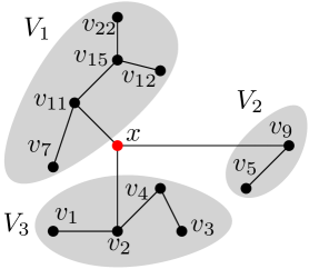
   Figure 1: Illustration of Definition 1 and Property 5. $V$ is the entire set of tree vertices. The 3 branches of $V$ falling off of $x$ are $V_{1},V_{2},V_{3}$. The cost of servicing branch $V_{i}$ is $f(V_{i}\cup\{x\},x)$. The cost of servicing the entire tree is $f(V,x)=\max_{1\leq i\leq 3}f(V_{i}\cup\{x\},x).$

Note that 1-5 only define a cost function over one subtree and one single sink. Function $f(\cdot,\,\cdot)$ is now naturally extended to work on on partitions and sets.

1. Max Partition Composition (Fig. 2)
   

   $$\forall\mathcal{P}\in\Lambda[X],\quad f(\mathcal{P},X)=\max_{1\leq i\leq|X|}f(P_{i},x_{i}).$$ (1)

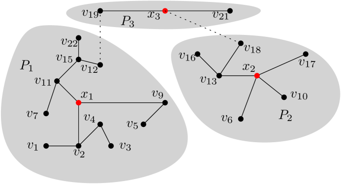
Figure 2: Illustration of Definition 1 and Property 6. The complete tree has been partitioned into $\mathcal{P}=(P_{1},P_{2},P_{3})$ with associated centers $X=(x_{1},x_{2},x_{3}).$ The cost associated with $(\mathcal{P},X)$ is $\max_{i=1,2,3}f(P_{i},x_{i})$.

Definition 2.

A cost function $f(\cdot,\,\cdot)$ on $T$ that satisfies properties 1-6 is called minmax monotone.

Finding a set of $k$ sinks $X$ and $\mathcal{P}\in\Lambda[X]$ that minimizes $f(\mathcal{P},X)$ is the minmax $k$-center tree partitioning problem, $k$-center partitioning for short. [15] describes a generic technique for solving this problem given an oracle for calculating the cost of a one sink solution given the sink location.

Definition 3.

Let $T=(V,E)$ be the input tree.

$\mathcal{A}$ is an oracle for $f(\cdot,\,\cdot)$ if, for all subtrees $T^{\prime}=(V^{\prime},E^{\prime})$ of $T$ and $x\in V^{\prime}$, $\mathcal{A}$ calculates $f(V^{\prime},x).$

$t_{\mathcal{A}}(n^{\prime})$ denotes the worst case time required for $\mathcal{A}$ to calculate $f(V^{\prime},x)$ for a subtree of size $n^{\prime}=|V^{\prime}|.$ $\mathcal{A}$ is asymptotically subadditive if

• $t_{\mathcal{A}}(n^{\prime})=\Omega(n^{\prime})$ and is non-decreasing.

• For all nonnegative $n_{i}$, $\sum_{i}t_{\mathcal{A}}(n_{i})=O\left(t_{\mathcal{A}}\Bigl{(}\sum_{i}n_{i}\Bigr{)}\right).$

• $t_{\mathcal{A}}(n^{\prime}+1)=O\left(t_{\mathcal{A}}(n^{\prime})\right)$.

Note that for $x\geq 1$ and $y\geq 0$ any function of the form $n^{x}\log^{y}n$ is asymptotically subadditive.

Theorem 2 ([15]).

Let $f(\cdot,\,\cdot)$ be a monotone minmax function and $\mathcal{A}$ an asymptotically subadditive oracle for $f(\cdot,\,\cdot).$ Then the $k$-center partitioning problem on $T$ can be solved in time

$$O\bigl{(}\max(k,\log n)kt_{\mathcal{A}}(n)\log^{2}n\bigr{)}.$$

2.1 Dynamic Confluent Flows on Trees – Evacuation protocols

The formal input to this problem is a tree $T=(V,E)$ along with

• A scenario $s=(w_{v_{1}}(s),w_{v_{2}}(s),\ldots,w_{v_{n}}(s))$.
  The problem starts with $w_{v_{i}}(s)\geq 0$ “units” of flow items located on vertex $v_{i}\in V$. All of this flow needs to be evacuated (moved) to some sink.

• For every edge $e=(u,v)\in E$, an associated length $d(u,v)>0$, denoting the time it takes a particle of flow to travel from $u$ to $v$. For $(u,v)\not\in E,$ $d(u,v)$ is defined to be the sum of the lengths of the edges on the unique path in $T$ connecting $u$ and $v.$

• A capacity $c>0$, denoting the rate, i.e., amount of flow that can enter an edge in one unit of time.

To move $w$ units of flow along edge $e=(u,v)$ from $u$ to $v$ note that the last particle of flow requires waiting $w/c$ units of time to enter $e$. After travelling along $e$ it finally arrives at $v$ at time $\frac{w}{c}+d(u,v).$

Let $T^{\prime}=(V^{\prime},E^{\prime})$ be some subtree of $T$ with $x\in V^{\prime}.$ $\Theta(V^{\prime},x:s)$ denotes the time required to evacuate all $w_{v^{\prime}}(s)$ flow on all $v^{\prime}\in V^{\prime}$ to sink $x$. This is the last time at which a particle of flow reaches $x.$

Congestion occurs when too many items are waiting to enter an edge. Congestion can build up if items arrive at a vertex faster than the rate ($c$) at which they leave it. This can happen if multiple edges feed into one vertex. The formula for $\Theta(V^{\prime},x:s)$ has been derived by multiple authors, e.g., [34, 29] in different ways. The version below is modified from [26].

Definition 4.

Let $T^{\prime}=(V^{\prime},E^{\prime})$ be a subtree and $x\not\in V^{\prime}$ be a neighbor of some node in $V^{\prime}$. For every $v^{\prime}\in V^{\prime},$ define

$$D(V^{\prime},x,v^{\prime})=\{v\in V^{\prime}\,:\,d(v,x)\geq d(v^{\prime},x)\}$$ (2)

Further set

$$W(V^{\prime},x,v:s)=\sum_{v\in D(V^{\prime},x,v^{\prime})}w_{v}(s).$$ (3)

Lemma 1.

Let $T^{\prime}=(V^{\prime},E^{\prime})$ be a subtree of $T$ and $x\not\in V^{\prime}$ be a neighbor of some node in $V^{\prime}$. Then

$$\Theta(V^{\prime}\cup\{x\},x:s)=\max_{v^{\prime}\in V^{\prime}:W(V^{\prime},x,v^{\prime}:s)>0}\left(d(v^{\prime},x)+\frac{W(V^{\prime},x,v^{\prime}:s)}{c}\right)$$ (4)

Figure 3: Example of evacuation to sink $x.$All edges have capacity $c=2.$ Edge lengths are next to the edge. Veterx indices are sorted by increasing length from $x.$ Vertex weights $w_{v}$ are not on the graph but are shown in the accompanying table. $W(v_{i})=\sum{v:d(x,v)\geq d(x,v_{i}}w(v).$ The rightmost column shows the values compared in (4). Note that the cost of the tree is 30, which is when the last item will reach $x.$

Note: For physical intuition, sort the nodes by increasing distance from $x$. For simplicity we will assume that all of the $d(v,x)$ values are unique and $d(v_{i},x)<d(v_{j},x)$ for $i<j.$ Without loss of generality assume that when particles from $v_{i}$ and $v_{j}$ with $i<j$ arrive at the head of some edge $e=(u,v)$ the particles from $v_{i}$ will enter $e$ before any particles from $v_{j}.$ On the path from $v$ to $x$ all flow from $v_{i}$ will remain ahead of all flow from $v_{j}$ and those two flows will remain in the same continuous stream. Thus flow will arrive at $x$ in continuous groups with time separating the tail item of one group from the head item of the next one. It is not difficult to work out that a group will contain all the flow that starts at a contiguous set of nodes $v_{i},v_{i+1},\ldots,v_{j}.$

$\Theta(V^{\prime}\cup\{x\},x:s)$ is the time that the last particle in the last group arrives at $x.$ Let $v^{\prime}$ be the first node in that last group. This last group will then contain exactly all the flow from nodes at distance $\geq d(x,v^{\prime})$ or further, i.e, the set $D(V^{\prime},x,v^{\prime})$ , which has in total $W=W(V^{\prime},x,v^{\prime}:s)$ flow. Since the first particle from $v^{\prime}$ will never experience congestion (if it did it would not be the first particle of a group) it arrives at $x$ at time $d(v^{\prime},x)$. The remaining items arrive continuously at rate $c,$ so the last item in the group will arrive at $x$ at time $W/c+d(v^{\prime},x)$, which is what (4) is indicating.

The function $\Theta(\cdot,\,\cdot:s)$ trivially satisfies properties 1-4 in the previous section. To see that it also satisfies property 5, let $V_{1},V_{2},\ldots,V_{t}$ be the branches of $V^{\prime}$ falling off of $x.$ Since $x$ has a unique neighbor $u_{i}\in V_{i}$, all items in $V_{i}$ evacuating to $x$ must pass through edge $(u_{i},x)$ and do not interact at all with items from any other subtree $V_{j},$ $j\not=i$ that are also evacuating to $x.$ Thus

$$\Theta(V^{\prime},x:s)=\max_{1\leq i\leq t}(\Theta(V_{i}\cup\{x\},x:s))$$

and $\Theta(V^{\prime},x:s)$ satisfies property 5. It is now extended naturally to work on partitions and sets.

Definition 5.

For any set of $k$ sinks $X$ and partition $\mathcal{P}\in\Lambda[X]$ define

$$\Theta(\mathcal{P},X:s)=\max\{\Theta(P_{1},x_{1}:s),\Theta(P_{2},x_{2}:s),\ldots,\Theta(P_{k},x_{k}:s)\}.$$

Further define

$$\Theta_{{\rm k-OPT}}(s)=\min\bigl{\{}\Theta(\mathcal{P},X:s)\,:\,|X|=k\mbox{ and }\mathcal{P}\in\Lambda[X]\bigr{\}}$$

to be the minimum time required to evacuate all items. The $(\mathcal{P},X)$ pair achieving this value is an optimal evacuation protocol. When $k$ is fixed and understood we will write $\Theta_{\rm OPT}$ instead of $\Theta_{{\rm k-OPT}}$.

Intuitively, $(\mathcal{P},X)$ denotes that $T$ is partitioned into subtrees, each containing one sink to which all flow in the subtree evacuates. $\Theta(\mathcal{P},X:s)$ is the time required to evacuate all of the items with $(\mathcal{P},X)$ under scenario $s.$ $\Theta_{\rm OPT}(s)$ is the minimum time required to evacuate the entire tree if it is $k$-partitioned.

Lemma 1 gives an immediate $O(n^{\prime}\log n^{\prime})$ oracle for solving the rooted one-sink version of the problem. Use an $O(n^{\prime})$ breadth first search starting at $x$ to separate $V^{\prime}$ into its branches. For each branch $V_{i}$, calculate the $d(v^{\prime},x)$ for $v^{\prime}\in V_{i}$, sort them in $O(|V_{i}|\log|V_{i}|)$ by increasing value and calculate $\Theta(V^{\prime}\cup\{x\},x:s)$ in $O(|V_{i}|)$ using brute force. Then return the maximum over all of the branch values. By plugging this $t_{\mathcal{A}}(n^{\prime})=O(n^{\prime}\log n^{\prime})$ oracle into Theorem 2, [15] derived

Theorem 3.

[15] There is an algorithm that solves the $k$-sink location problem on trees with uniform capacity in

$$O(\max(k,\log n)\,kn\log^{3}n)$$

time.

3 Regret

In a minmax-regret model on trees, the input tree $T$ is given but some of the other input values are not fully known in advance. The input specifies restrictions on the allowed values for the missing inputs.

Concretely, in the minmax-regret $k$-sink evacuation problem on trees the input tree $T$, capacity $c$ and lengths $d(u,v)$ are all explicitly specified as part of the input. The weights $w_{v}$ are not fully specified in advance. Instead, for each $v\in V$, a range $[w_{i}^{-},w_{i}^{+}]$ within which $w_{i}$ must lie is specified. The set of all possible allowed scenarios is the Cartesian product of all weight intervals,

$$\mathcal{S}=\prod_{v\in V}[w_{v}^{-},w_{v}^{+}],$$

$s\in\mathcal{S}$ is an assignment of weights to all vertices. The weight of a vertex $v$ under scenario $s$ is denoted by $w_{v}(s)$.

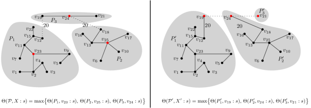
Figure 4: Illustration of regret. Capacity $c=1$. All edges have length $d(u,v)=1$ except for $d(v_{12},v_{19})=d(v_{18},v_{24})=20.$ For all vertices $v_{i}$ except for $i=19,21,24$, $[w^{-}_{v_{i}},w^{+}_{v_{i}}]=[1,2]$. For $i=19,21,24$, $[w^{-}_{v_{i}},w^{+}_{v_{i}}]=[1,100]$. Let $s^{*}$ be a scenario for which $w_{v}(s^{*})=1$ for all $v$ except for $w_{v_{19}}(s^{*})=w_{v_{21}}(s^{*})=w_{v_{24}}(s^{*})=100.$ Then $\Theta(\mathcal{P},X:s^{*})=\Theta(P_{3},v_{24}:s^{*})=101.$ A little calculation shows that $\Theta(\mathcal{P}^{\prime},X^{\prime}:s^{*})=\Theta(P_{1},v_{19}:s^{*})=30=\Theta_{\rm OPT}(s^{*}).$ So $R(\mathcal{P},X:s)=101-30=71.$ It is not that difficult to show that this $s^{*}$ is a worst case scenario for $(\mathcal{P},X)$ so $R_{\max}(\mathcal{P},X)=71.$

Definition 6 (Regret for $(\mathcal{P},X)$ under scenario $s$).

For fixed $(\mathcal{P},X)$ with $|X|=k$ and $s\in\cal{S}$, the regret is defined as the difference between $\Theta(\mathcal{P},X:s)$ and the optimal $k$-Sink evacuation time for $s,$ i.e.,

$$R(\mathcal{P},X:s)=\Theta(\mathcal{P},X:s)-\Theta_{{\rm k-OPT}}(s).$$ (5)

Definition 7 (Max-Regret for $(P,X)$).

The Maximum-Regret achieved (over all scenarios) for a choice of $(P,X)$ is

$$R_{\max}(\mathcal{P},X)=\max_{s\in\mathcal{S}}\left\{R(\mathcal{P},X:s)\right\}.$$ (6)

$s^{*}\in\mathcal{S}$ is a worst-case scenario for $(P,X)$ if $R_{\max}(\mathcal{P},X)=R(\mathcal{P},X:s^{*}).$

Finally, set

Definition 8 (Global Minmax-Regret).

Let $k$ be fixed.

$$R_{\rm OPT}=\min_{(\mathcal{P},X):|X|=k}R_{\max}(\mathcal{P},X).$$

$(\mathcal{P}^{*},X^{*})$ is an optimal minmax-regret evacuation protocol if $R_{\rm OPT}=R_{\max}(\mathcal{P}^{*},X^{*})$.

For later we use we note that, by definition, $R_{\max}(\mathcal{P},X)\geq 0$, and thus

Lemma 2.

$$\forall X\subseteq V\mbox{\rm and }\mathcal{P}\in\Lambda[X],\quad R_{\max}(\mathcal{P},X)\geq 0.$$

3.1 Minmax-Regret $k$-Sink Location Problem

As described above, the input for the Minmax-Regret $k$-Sink Location Problem is a dynamic flow tree network with edge lengths, vertex weight intervals $[w_{i}^{-},w_{i}^{+}]$ and edge capacity $c$. The goal is calculate $R_{\rm OPT}$ along with a corresponding optimal minmax-regret evacuation protocol $(\mathcal{P}^{*},X^{*})$ with associated worst case scenario $s^{*}.$

This setup can be viewed as a 2-person Stackelberg game between the algorithm $A$ and adversary $B$:

1. Algorithm $A$ (leader): creates an evacuation protocol $(\mathcal{P},X)$.

2. Adversary $B$ (follower): chooses a worst-case scenario $s^{*}\in\mathcal{S}$ for $(\mathcal{P},X)$ i.e., $R(\mathcal{P},X:s^{*})=R_{\max}(\mathcal{P},X)$.

$A$’s objective is to minimize the value of $R(\mathcal{P},X:s^{*})$ which is equivalent to finding optimal minmax-regret evacuation protocol $(\mathcal{P}^{*},X^{*}).$

Note that even though we have defined regret only for the $k$-sink evacuation problem, this formulation can be (and has been) extended to many other problems by replacing $\Theta$ with any other minmax monotone function.

4 Worst Case Scenario Properties

The explicit formula for evacuation time given by Eq. 4 in Lemma 1 immediately implies

Lemma 3.

Let $s,s^{\prime}\in\mathcal{S}$ be two scenarios such that $\forall v\in V,w_{v}(s^{\prime})\leq w_{v}(s)$.

1. If $T^{\prime}=(V^{\prime},E^{\prime})$ is a subtree of $T$ and $x\in V^{\prime}.$

   $$\Theta(V^{\prime},x:s^{\prime})\leq\Theta(V^{\prime},x:s).$$

2. $\Theta_{\rm OPT}(s^{\prime})\leq\Theta_{\rm OPT}(s).$

Eq. 4 in Lemma 1 also immediately implies

Lemma 4.

Let $s$ be a scenario and $s^{\prime}$ be another scenario such that, for some $v^{\prime}\in V$, and some $\delta>0$

$$w_{v}(s^{\prime})=\left\{\begin{array}[]{cc}w_{v}(s)&\mbox{if $v\not=v^{\prime}$},\\ w_{v}(s)+\delta&\mbox{if $v=v^{\prime}$}.\end{array}\right.$$

Then

$$\Theta_{\rm OPT}(s^{\prime})\leq\Theta_{\rm OPT}(s)+\frac{\delta}{c}.$$

Definition 9 (Dominant Subtrees and Branches).

$P_{i}\in\mathcal{P}$ is a dominant subtree for $(\mathcal{P},X)$ under scenario $s$ if

$$\Theta(\mathcal{P},X:s)=\Theta(P_{i},x_{i}:s).$$

For any $P_{i}$, a dominant branch of $P_{i}$ falling off of $x_{i}$ is a branch $V_{j}$ of $P_{i}$ falling off of $x_{i}$ such that

$$\Theta(P_{i},x_{i}:s)=\Theta(V_{j}\cup\{x_{i}\},x_{i}:s).$$

Note that, by this definition, if $s^{*}\in\mathcal{S}$ is a worst-case scenario for $(\mathcal{P},X)$ and $P_{i}\in\mathcal{P}$ is a dominant subtree for $(\mathcal{P},X)$ under scenario $s^{*}$ then

$$R_{\max}(\mathcal{P},X)=\Theta(\mathcal{P},X:s^{*})-\Theta_{\rm OPT}(s^{*})=\Theta(P_{i},x_{i}:s^{*})-\Theta_{\rm OPT}(s^{*}).$$

Furthermore, if $V_{j}$ is a dominant branch of that $P_{i}$ falling off of $x_{i}$ under $s$ then

$$R_{\max}(\mathcal{P},X)=\Theta(P_{i},x_{i}:s^{*})-\Theta_{\rm OPT}(s^{*})=\Theta(V_{j}\cup\{x_{i}\},x_{i}:s)-\Theta_{\rm OPT}(s^{*}).$$

Figure 5: Illustration of Definition 10. The edge lengths are only explicitly given for the subtree $V_{2}$. The scenario $s^{*}=s^{*}(V_{2},x,v_{5})$ is illustrated. All vertices labelled with a “+”have $s^{*}(v)=w^{+}_{v}.$ Since $d(x,v_{5})=12$, these are the vertices $v^{\prime}\in V_{2}$ such that $d(x,v^{\prime})\geq 12.$ All other vertices are labelled with a “-” and have $s^{*}(v)=w^{-}_{v}.$

Definition 10.

1. Let $V^{\prime}\subseteq V$ ($V^{\prime}$ is not necessarily a tree). Set $s^{*}(V^{\prime})$ to be the scenario such that

   $$w_{v}(s^{*}(V^{\prime}))=\left\{\begin{array}[]{cc}w^{-}_{v}&\mbox{if $v\not\in V^{\prime}$}\\ w^{+}_{v}&\mbox{if $v\in V^{\prime}.$}\end{array}\right.$$

   Note that, $\forall v\in V,$ $w_{v}(s^{*}(\emptyset))=w^{-}_{v}.$

2. Let $T^{\prime}=(V^{\prime},E^{\prime})$ be a subtree with $x\in V^{\prime}$ and $V_{1},...,V_{t}$ be the branches of $V^{\prime}$ falling off of $x.$ Now set (Fig. 5)

   $$\mathcal{S}^{*}(V^{\prime},x)=s^{*}(\emptyset)\cup\bigcup_{j=1}^{t}\left\{s^{*}(D(V_{j},x,v^{\prime}))\,:\,v^{\prime}\in V_{j}\right\}$$

   where $D(V_{j},x,v^{\prime})$ is as introduced in Definition 4.

3. Set

   $$\mathcal{S}^{*}(\mathcal{P},X)=\bigcup_{i=1}^{k}\mathcal{S}^{*}(P_{i},x_{i}).$$

Note that $\mathcal{S}^{*}(V^{\prime},x)$ contains at most one scenario associated with each $v\in V^{\prime}$ (associate $s^{*}(\emptyset)$ with $x$) and thus $|\mathcal{S}^{*}(V^{\prime},x)|\leq|V^{\prime}|$ and $|\mathcal{S}^{*}(\mathcal{P},X)|\leq n.$ The main result is

Lemma 5.

Let $s\in\mathcal{S}$ be a worst case scenario for $(\mathcal{P},X)$ and $P_{i}\in\mathcal{P}$ be a dominant subtree for $(\mathcal{P},X)$ under scenario $s$. Furthermore, let $V_{j}$ be a dominant branch in $P_{i}$ falling off of $x_{i}$ under $s$.

Then there exists some $s^{*}\in\mathcal{S}^{*}(V_{j}\cup\{x_{i}\},x_{i})\subseteq\mathcal{S}^{*}(P_{i},x_{i})$ such that

1. $s^{*}$ is also a worst case scenario for $(\mathcal{P},X)$ and

2. $P_{i}\in\mathcal{P}$ is a dominant subtree for $(\mathcal{P},X)$ under scenario $s^{*}$,

3. with $V_{j}$ being a dominant branch of $P_{i}$ falling off of $x_{i}$ under $s^{*}.$

Furthermore

$$R_{\max}(\mathcal{P},X)=\Theta(\mathcal{P},X:s^{*})-\Theta_{\rm OPT}(s^{*}) = \Theta(P_{i},x_{i}:s^{*})-\Theta_{\rm OPT}(s^{*})$$

$$= \Theta(V_{j}\cup\{x_{i}\},x_{i}:s^{*})-\Theta_{\rm OPT}(s^{*}).$$

Proof.

By definition, $\mathcal{P},X,s$ satisfy

$$R_{\max}(\mathcal{P},X)=\Theta(P_{i},x_{i}:s)-\Theta_{\rm OPT}(s).$$

Now let $V_{1},\ldots,V_{t}$ be the branches of $P_{i}$ hanging off of $x_{i}$ and let $V_{j}$ be a dominant branch of $P_{i}$ under $s.$ Then

$$\Theta(P_{i},x_{i}:s)=\max_{1\leq\ell\leq t}\Theta(V_{\ell}\cup\{x_{i}\},x_{i}:s)=\Theta(V_{j}\cup\{x_{i}\},x_{i}:s)$$

(a) Reducing $w$ values outside of dominant branch:
Define $s^{\prime}$ such that

$$w_{v}(s^{\prime})=\left\{\begin{array}[]{cc}w^{-}_{v}&\mbox{if $v\not\in V_{j}$,}\\ w_{v}(s)&\mbox{if $v\in V_{j}$.}\end{array}\right.$$

From Lemma 3(1),

$$\forall i^{\prime}\not=i,\quad\Theta(P_{i^{\prime}},x_{i^{\prime}}:s^{\prime})\leq\Theta(P_{i^{\prime}},x_{i^{\prime}}:s)\quad\mbox{ and }\quad\forall\ell\not=j,\quad\Theta(V_{\ell}\cup\{x_{i}\},x_{i}:s^{\prime})\leq\Theta(V_{\ell}\cup\{x_{i}\},x_{i}:s).$$

Since $s$ and $s^{\prime}$ are identical within $V_{j},$

$$\Theta(V_{j}\cup\{x_{i}\},x_{i}:s^{\prime})=\Theta(V_{j}\cup\{x_{i}\},x_{i}:s).$$

Thus

$$\Theta(P_{i},x_{i}:s^{\prime})=\max_{1\leq\ell\leq t}\Theta(V^{\prime}_{\ell}\cup\{x_{i}\},x_{i}:s^{\prime})=\Theta(V_{j}\cup\{x_{i}\},x_{i}:s)=\Theta(P_{i},x_{i}:s)$$

and

$$\Theta(\mathcal{P},X:s^{\prime})=\Theta(P_{i},x_{i}:s^{\prime})=\Theta(P_{i},x_{i}:s)=\Theta(\mathcal{P},X:s).$$

From Lemma 3 (2),

$$\Theta_{\rm OPT}(s^{\prime})\leq\Theta_{\rm OPT}(s)$$

and thus

$$\Theta(\mathcal{P},X:s^{\prime})-\Theta_{\rm OPT}(s^{\prime})\geq\Theta(\mathcal{P},X:s)-\Theta_{\rm OPT}(s)=R_{\max}(\mathcal{P},X).$$

From Definition 7, $\Theta(\mathcal{P},X:s^{\prime})-\Theta_{\rm OPT}(s^{\prime})\leq R_{\max}(\mathcal{P},X)$ and thus

$$R_{\max}(\mathcal{P},X)=\Theta(P_{i},x_{i}:s^{\prime})-\Theta_{\rm OPT}(s^{\prime}).$$

This implies $s^{\prime}$ is also a worst case scenario for $(\mathcal{P},X)$ with $P_{i}\in\mathcal{P}$ a dominant subtree for $(\mathcal{P},X)$ under scenario $s^{\prime}$, with $V_{j}$ a dominant branch in $P_{i}$.

(b) Reducing $w$ values inside of dominant branch:
Recall from Lemma 1  that

$$\Theta(V_{j}\cup\{x_{i}\},x_{i}:s^{\prime})=\max_{v^{\prime}\in V_{j}:W(V_{j},x_{i},v^{\prime}:s^{\prime})>0}\left(d(v^{\prime},x_{i})+\frac{W(V_{j},x_{i},v^{\prime}:s^{\prime})}{c}\right).$$

Let $\bar{v}\in V_{j}$ be any vertex (if ties occur, there might be many) such that

$$\Theta(V_{j}\cup\{x_{i}\},x_{i}:s^{\prime})=d(\bar{v},x_{i})+\frac{W(V_{j},x_{i},\bar{v}:s^{\prime})}{c}.$$ (8)

Now let $v^{\prime\prime}\in V_{j}$ such that $d(v^{\prime\prime},x_{i})<d(\bar{v},x_{i})$. Transform $s^{\prime}$ into $s^{\prime\prime}$ by setting

$$w_{v}(s^{\prime\prime})=\left\{\begin{array}[]{cc}w^{-}_{v}&\mbox{if $v=v^{\prime\prime}$,}\\ w_{v}(s^{\prime})&\mbox{if $v\not=v^{\prime\prime}$.}\end{array}\right.$$

We now show that $s^{\prime\prime}$ will remain a worst case scenario with the same properties.

Because $w_{v}(s^{\prime\prime})=w_{v}(s^{\prime})$ for all $v\not\in V_{j}$ we have

$$\forall i^{\prime}\not=i,\quad\Theta(P_{i^{\prime}},x_{i^{\prime}}:s^{\prime\prime})=\Theta(P_{i^{\prime}},x_{i^{\prime}}:s^{\prime})\quad\mbox{ and }\quad\forall\ell\not=j,\quad\Theta(V_{\ell}\cup\{x_{i}\},x_{i}:s^{\prime\prime})=\Theta(V_{\ell}\cup\{x_{i}\},x_{i}:s^{\prime}).$$

Now note that, for all $v^{\prime}\in V_{j}$, the weight change implies

$$W(V_{j},x_{i},v^{\prime}:s^{\prime\prime})=\left\{\begin{array}[]{ll}W(V_{j},x_{i},v^{\prime}:s^{\prime})-(w_{v^{\prime\prime}}(s^{\prime})-w^{-}_{v^{\prime\prime}})&\mbox{if $d(v^{\prime},x)\leq d(v^{\prime\prime},x)$},\\ W(V_{j},x_{i},v^{\prime}:s^{\prime})&\mbox{if $d(v^{\prime},x)>d(v^{\prime\prime},x)$}.\end{array}\right.$$

Since $d(\bar{v},x)>d(v^{\prime\prime},x)$, $W(V_{j},x_{i},\bar{v}:s^{\prime\prime})=W(V_{j},x_{i},\bar{v}:s^{\prime})$ and

$$\Theta(V_{j}\cup\{x_{i}\},x_{i}:s^{\prime\prime}) = \max_{v^{\prime}\in V_{j}:W(V_{j},x_{i},v^{\prime}:s^{\prime\prime})>0}\left(d(v^{\prime},x_{i})+\frac{W(V_{j},x_{i},v^{\prime}:s^{\prime\prime})}{c}\right)$$

$$= d(\bar{v},x_{i})+\frac{W(V_{j},x_{i},\bar{v}:s^{\prime\prime})}{c}$$

$$= d(\bar{v},x_{i})+\frac{W(V_{j},x_{i},\bar{v}:s^{\prime})}{c}$$

$$= \Theta(V_{j}\cup\{x_{i}\},x_{i}:s^{\prime})$$

Thus, exactly as in (a),

$$\Theta(P_{i},x_{i}:s^{\prime\prime})=\max_{1\leq\ell\leq t}\Theta(V^{\prime}_{\ell}\cup\{x_{i}\},x_{i}:s^{\prime\prime})=\Theta(V_{j}\cup\{x_{i}\},x_{i}:s^{\prime})=\Theta(P_{i},x_{i}:s^{\prime})$$

and

$$\Theta(\mathcal{P},X:s^{\prime\prime})=\Theta(P_{i},x_{i}:s^{\prime\prime})=\Theta(P_{i},x_{i}:s^{\prime})=\Theta(\mathcal{P},X:s^{\prime}).$$

Again from Lemma 3 (2),

$$\Theta_{\rm OPT}(s^{\prime\prime})\leq\Theta_{\rm OPT}(s^{\prime})$$

and using the same argument as in (a),

$$R_{\max}(\mathcal{P},X)=\Theta(P_{i},x_{i}:s^{\prime\prime})-\Theta_{\rm OPT}(s^{\prime\prime}).$$

This again implies $s^{\prime\prime}$ is also a worst case scenario for $(\mathcal{P},X)$ with $P_{i}\in\mathcal{P}$ a dominant subtree for $(\mathcal{P},X)$ under scenario $s^{\prime\prime}$, with $V_{j}$ a dominant branch in $P_{i}$.

Now, set $s^{\prime}$ to be $s^{\prime\prime}$. The argument above can be repeated for every $v^{\prime\prime}\in V_{j}$ with $d(v^{\prime\prime},x)<d(\bar{v},x)$ and thus we may assume that for all such $v^{\prime\prime}\in V_{j}$, $w_{v^{\prime\prime}}(s^{\prime})=w^{-}_{v^{\prime\prime}}.$

(c) Increasing $w$ values inside of dominant branch:
Let $\bar{v}$ be as defined in Eq. (8) from (b) but now let $v^{\prime\prime}\in V_{j}$ be any vertex such that $d(v^{\prime\prime},x_{i})\geq d(\bar{v},x_{i})$. Suppose that $w_{v^{\prime\prime}}(s^{\prime})<w^{+}_{v^{\prime}}$. Transform $s^{\prime}$ into $s^{\prime\prime}$ by

$$w_{v}(s^{\prime\prime})=\left\{\begin{array}[]{cc}w_{v}(s^{\prime})&\mbox{if $v\not=v$,}\\ w^{+}_{v^{\prime\prime}}&\mbox{if $v=v^{\prime\prime}$.}\end{array}\right.$$

We now show that $s^{\prime\prime}$ will still remain a worst case scenario with the same properties.

Similar to part (b), since $w_{v}(s^{\prime\prime})=w_{v}(s^{\prime})$ for all $v\not\in V_{j}$ we have

$$\forall i^{\prime}\not=i,\quad\Theta(P_{i^{\prime}},x_{i^{\prime}}:s^{\prime})=\Theta(P_{i^{\prime}},x_{i^{\prime}}:s)\quad\mbox{ and }\quad\forall j^{\prime}\not=j,\quad\Theta(V_{j^{\prime}}\cup\{x_{i}\},x_{i}:s^{\prime})=\Theta(V_{\ell}\cup\{x_{i}\},x_{i}:s).$$

Now note that for all $v^{\prime}\in V_{j}$, the weight change implies

$$W(V_{j},x_{i},v^{\prime}:s^{\prime\prime})=\left\{\begin{array}[]{ll}W(V_{j},x_{i},v^{\prime}:s^{\prime})+(w^{+}_{v^{\prime\prime}}-w_{v^{\prime\prime}}(s^{\prime}))&\mbox{if $d(v^{\prime},x)\leq d(v^{\prime\prime},x)$},\\ W(V_{j},x_{i},v^{\prime}:s^{\prime})&\mbox{if $d(v^{\prime},x)>d(v^{\prime\prime},x)$}.\end{array}\right.$$

Thus $W(V_{j},x_{i},\bar{v}:s^{\prime\prime})=W(V_{j},x_{i},\bar{v}:s^{\prime})+(w^{+}_{v^{\prime\prime}}-w_{v^{\prime\prime}}(s^{\prime}))$ and

$$\Theta(V_{j}\cup\{x_{i}\},x_{i}:s^{\prime\prime}) = \max_{v^{\prime}\in V_{j}:W(V_{j},x_{i},v^{\prime}:s^{\prime\prime})>0}\left(d(v^{\prime},x_{i})+\frac{W(V_{j},x_{i},v^{\prime}:s^{\prime\prime})}{c}\right)$$

$$= d(\bar{v},x_{i})+\frac{W(V_{j},x_{i},\bar{v}:s^{\prime\prime})}{c}$$

$$= d(\bar{v},x_{i})+\frac{W(V_{j},x_{i},\bar{v}:s^{\prime})}{c}+\frac{(w^{+}_{v^{\prime\prime}}-w_{v^{\prime\prime}}(s^{\prime}))}{c}$$

$$= \Theta(V_{j}\cup\{x_{i}\},x_{i}:s^{\prime})+\frac{(w^{+}_{v^{\prime\prime}}-w_{v^{\prime\prime}}(s^{\prime}))}{c}$$

Then,

$$\Theta(P_{i},x_{i}:s^{\prime\prime})=\max_{1\leq\ell\leq t}\Theta(V^{\prime}_{\ell}\cup\{x_{i}\},x_{i}:s^{\prime\prime})=\Theta(P_{i},x_{i}:s^{\prime})+\frac{(w^{+}_{v^{\prime\prime}}-w_{v^{\prime\prime}}(s^{\prime}))}{c}$$

and

$$\Theta(\mathcal{P},X:s^{\prime\prime})=\Theta(P_{i},x_{i}:s^{\prime\prime})=\Theta(\mathcal{P},X:s^{\prime})+\frac{(w^{+}_{v^{\prime\prime}}-w_{v^{\prime\prime}}(s^{\prime}))}{c}.$$

From Lemma 4,

$$\Theta_{\rm OPT}(s^{\prime\prime})\leq\Theta_{\rm OPT}(s^{\prime})+\frac{(w^{+}_{v^{\prime\prime}}-w_{v^{\prime\prime}}(s^{\prime}))}{c}.$$

Thus,

$$\Theta(\mathcal{P},X:s^{\prime\prime})-\Theta_{\rm OPT}(s^{\prime\prime}) = \left(\Theta(\mathcal{P},X:s^{\prime})+\frac{(w^{+}_{v}-w_{v^{\prime\prime}}(s^{\prime}))}{c}\right)-\Theta_{\rm OPT}(s^{\prime\prime})$$

$$\geq \left(\Theta(\mathcal{P},X:s^{\prime})+\frac{(w^{+}_{v}-w_{v^{\prime\prime}}(s^{\prime}))}{c}\right)-\left(\Theta_{\rm OPT}(s^{\prime})+\frac{(w^{+}_{v}-w_{v^{\prime\prime}}(s^{\prime}))}{c}\right)$$

$$= \Theta(\mathcal{P},X:s^{\prime})-\Theta_{\rm OPT}(s^{\prime})=R_{\max}(\mathcal{P},X).$$

The definition of $R_{\max}(\mathcal{P},X)$ guarantees that $\Theta(\mathcal{P},X:s^{\prime\prime})-\Theta_{\rm OPT}(s^{\prime\prime})\leq R_{\max}(\mathcal{P},X)$ and thus

$$R_{\max}(\mathcal{P},X)=\Theta(P_{i},x_{i}:s^{\prime\prime})-\Theta_{\rm OPT}(s^{\prime}).$$

This implies that $s^{\prime\prime}$ is again a worst case scenario for $(\mathcal{P},X)$ with $P_{i}\in\mathcal{P}$ a dominant subtree for $(\mathcal{P},X)$ under scenario $s^{\prime\prime}$, with $V_{j}$ a dominant branch in $P_{i}$.

Now, set $s^{\prime}$ to be $s^{\prime\prime}$. The argument above can be repeated for every $v^{\prime\prime}\in V_{j}$ with $d(v^{\prime\prime},x_{i})\geq d(\bar{v},x_{i})$ and thus we may assume, that for all such $v^{\prime\prime}\in V_{j}$, $w_{v^{\prime\prime}}(s^{\prime})=w^{+}_{v^{\prime\prime}}.$

(d) Wrapping up:
After applying (a) followed by (b) followed by (c) the final $s^{\prime}$ constructed is exactly

$$s^{\prime}=s^{*}(D(P_{i},x_{i},\bar{v})).$$

Since this $s^{\prime}\in\mathcal{S}^{*}(V_{j}\cup\{x_{i}\},x_{i})\subseteq\mathcal{S}^{*}(P_{i},x_{i})$ and satisfies properties (1) and (2) required by the Lemma, the proof is complete.

∎

5 The Local Max-Regret Function

Definition 11.

Let $T=(V,E)$ be a tree, $v\in V$ and $T^{\prime}=(V^{\prime},E^{\prime})$ a subtree of $T$. The relative max-regret function is

$$r(V^{\prime},x)=\max_{s\in\mathcal{S}^{*}(V^{\prime},x)}\left\{\Theta(V^{\prime},x:s)-\Theta_{\rm OPT}(s)\right\}$$

Let $X\subseteq V$ and $\mathcal{P}\in\Lambda[X].$ Set

$$r(\mathcal{P},X)=\max_{1\leq i\leq k}r(P_{i},x_{i}).$$ (9)

Recall that $|\mathcal{S}^{*}(V^{\prime},x)|\leq|V^{\prime}|$.This will permit efficiently calculating $r(\mathcal{P},X)$. Surprisingly, evne though $r(\mathcal{P},X)$ is a locally defined function, it encodes enough information to fully calculate the global value $R_{\max}(\mathcal{P},X)$.

Lemma 6 ($r(\cdot,\,\cdot)$ is almost min-max monotone).

• The function $r(\cdot,\,\cdot)$ satisfies properties 1-2 and 4–6 of Definition 2.

• Let $X\subseteq V$ and $\mathcal{P}\in\Lambda[X].$ Then

  $$r(\mathcal{P},X)=R_{\max}(\mathcal{P},X)$$

• $$R_{\rm OPT}=\min_{(\mathcal{P},X):|X|=k}R_{\max}(\mathcal{P},X)=\min_{(\mathcal{P},X):|X|=k}r(\mathcal{P},X)$$

Proof.

(a) For any fixed $s\in\mathcal{S}$ set

$$r^{\prime}(V^{\prime},x:s)=\Theta(V^{\prime},x:s)-\Theta_{\rm OPT}(s).$$

For fixed scenario $s,$ $\Theta(\cdot,\,\cdot:s)$ is minmax monotone. Properties 1,2 and 4 all remain invariant under the subtraction of a constant, so $r^{\prime}(\cdot,\,\cdot)$ also satisfies properties 1,2 and 4. Since $r(V^{\prime},x)=\max_{s\in\mathcal{S}^{*}(V^{\prime},x)}r^{\prime}(V^{\prime},x:s)$ and properties 1,2 and 4 also remain invariant under taking maximum, $r(\cdot,\,\cdot)$ also satisfies properties 1,2 and 4.

For property 5, let $T^{\prime}=(V^{\prime},E^{\prime})$ be a subtree of $T$, $x\in V^{\prime}$ and $V_{1},...,V_{t}$ the branches of $V^{\prime}$ falling off of $x.$ We first claim that

$$\forall\ell,\quad\max_{s\in\mathcal{S}^{*}(V_{\ell}\cup\{x\},x)}r^{\prime}(V_{\ell}\cup\{x\},x:s)=\max_{s\in\mathcal{S}^{*}(V^{\prime},x)}r^{\prime}(V_{\ell}\cup\{x\},x:s).$$ (10)

Suppose not. Then, for some $\ell$, there exists $\ell^{\prime}\not=\ell$ and $s^{*}\in\mathcal{S}^{*}(V_{\ell^{\prime}}\cup\{x\},x)$ such that

$$r^{\prime}(V_{\ell}\cup\{x\},x:s^{*})>\max_{s\in\mathcal{S}^{*}(V_{\ell}\cup\{x\},x)}r^{\prime}(V_{\ell}\cup\{x\},x:s).$$ (11)

Since $\ell\not=\ell^{\prime}$, for all $v^{\prime}\in V_{\ell},$ $w_{v^{\prime}}(s^{*})=w^{-}_{v^{\prime}}=w_{v^{\prime}}(s^{*}(\emptyset))$ and thus

$$\Theta(V_{\ell}\cup\{x\},x:s^{*}(\emptyset))=\Theta(V_{\ell}\cup\{x\},x:s^{*}).$$

Furthermore, by Lemma 3, $\Theta_{\rm OPT}(s^{*}(\emptyset))\leq\Theta_{\rm OPT}(s^{*}).$ Since $s^{*}(\emptyset)\in\mathcal{S}^{*}(V_{\ell}\cup\{x\},x),$ from Eq. (11),

$$\max_{s\in\mathcal{S}^{*}(V_{\ell}\cup\{x\},x)}r^{\prime}(V_{\ell}\cup\{x\},x:s) \geq r^{\prime}(V_{\ell}\cup\{x\},x:s(\emptyset))$$

$$= \Theta(V_{\ell}\cup\{x\},x:s^{*}(\emptyset))-\Theta_{\rm OPT}(s^{*}(\emptyset)$$

$$\geq \Theta(V_{\ell}\cup\{x\},x:s^{*})-\Theta_{\rm OPT}(s^{*})$$

$$= r^{\prime}(V_{\ell}\cup\{x\},x:s^{*})$$

contradicting (11). Thus (10) is proved. Next note

$$r(V^{\prime},x) = \max_{s\in\mathcal{S}^{*}(V^{\prime},x)}\left(\Theta(V^{\prime},x:s)-\Theta_{\rm OPT}(s)\right)$$

$$= \max_{s\in\mathcal{S}^{*}(V^{\prime},x)}\left(\max_{1\leq\ell\leq t}\Theta(V_{\ell}\cup\{x\},x:s)-\Theta_{\rm OPT}(s)\right)$$

$$= \max_{s\in\mathcal{S}^{*}(V^{\prime},x)}\left(\max_{1\leq\ell\leq t}r^{\prime}(V_{\ell}\cup\{x\},x:s).\right)$$

$$= \max_{1\leq\ell\leq t}\left(\max_{s\in\mathcal{S}^{*}(V^{\prime},x)}r^{\prime}(V_{\ell}\cup\{x\},x:s)\right)$$

$$= \max_{1\leq\ell\leq t}\left(\max_{s\in\mathcal{S}^{*}(V_{i}\cup\{x\},x)}r^{\prime}(V_{\ell}\cup\{x\},x:s)\right)\hskip 14.45377pt(\mbox{From Eq.~{}\ref{eq:sim}})$$

$$= \max_{1\leq\ell\leq t}r\left(V_{\ell}\cup\{x\},x\right).$$

$r(\cdot,\,\cdot)$ therefore satisfies Property 5. Property 6 follows by definition.

(b)

$$R_{\max}(\mathcal{P},X) = \max_{s\in\mathcal{S}}\Bigl{(}\Theta(\mathcal{P},X:s)-\Theta_{\rm OPT}(s)\Bigr{)}$$

$$= \max_{s\in\mathcal{S}}\left(\max_{1\leq i\leq k}\Theta(P_{i},x_{i}:s)-\Theta_{\rm OPT}(s)\right)$$

$$= \max_{s\in\mathcal{S}}\left(\max_{1\leq i\leq k}\Bigl{(}\Theta(P_{i},x_{i}:s)-\Theta_{\rm OPT}(s)\Bigr{)}\right)$$

$$= \max_{s\in\mathcal{S}}\left(\max_{1\leq i\leq k}r^{\prime}(P_{i},x_{i}:s)\right)$$

$$= \max_{1\leq i\leq k}\left(\max_{s\in\mathcal{S}}r^{\prime}(P_{i},x_{i}:s)\right)$$

$$\geq \max_{1\leq i\leq k}\left(\max_{s\in\mathcal{S}^{*}(P_{i},x)}r^{\prime}(P_{i},x_{i}:s)\right)\hskip 14.45377pt(\mbox{Because $\mathcal{S}^{*}(P_{i},x)\subseteq\mathcal{S}$ })$$

$$= \max_{1\leq i\leq k}r(P_{i},x_{i})$$

$$= r(\mathcal{P},X)$$

From Lemma 5 we know there exists a $s^{*}\in S^{*}(V^{\prime},x)$ and $P_{i}\in\mathcal{P}$ such that

$$R_{\max}(\mathcal{P},X)=\Theta(P_{i},x_{i}:s^{*})-\Theta_{\rm OPT}(s^{*})$$

Thus

$$R_{\max}(\mathcal{P},X)\leq r(P_{i},x_{i})\leq r(\mathcal{P},X)$$

and $R_{\max}(\mathcal{P},X)=r(\mathcal{P},X).$

(c) Follows directly from (b).

∎

The previous lemma states that $r(\cdot,\,\cdot)$ satisfies all of the properties of a minmax monotone function EXCEPT for property 3. Property 3 may be violated since it is quite possible that, for any particular $V^{\prime}$, that $r(V^{\prime},x)<0.$ As an example, suppose that $V^{\prime}={x}$, a singleton node. Since $\Theta(\{x\},x)=0$,

$$r(V^{\prime},x)=\max_{s\in\mathcal{S}^{*}(V^{\prime},x)}\left\{\Theta(V^{\prime},x:s)-\Theta_{\rm OPT}(s)\right\}=-\max_{s\in\mathcal{S}^{*}(V^{\prime},x)}\left\{\Theta_{\rm OPT}(s)\right\}$$

which other than in some special cases will be negative. Because of this $r(\cdot,\,\cdot)$ is not minmax monotone and Theorem 2 can’t be directly applied. This can be easily patched, though.

Lemma 7.

Let $T=(V,E)$ be a tree, $v\in V$ and $T^{\prime}=(V^{\prime},E^{\prime})$ a subtree of $T$. Set

$${\bar{r}}(V^{\prime},x)=\max(r(V^{\prime},x),\,0).$$

Now let $X\subseteq V$ and $\mathcal{P}\in\Lambda[X].$ Set

$${\bar{r}}(\mathcal{P},X)=\max_{1\leq i\leq k}{\bar{r}}(P_{i},x_{i}).$$

Then

• $\bar{r}(\cdot,\,\cdot)$ is a minmax monotone function.

• $$R_{\rm OPT}=\min_{(\mathcal{P},X):|X|=k}{\bar{r}}(\mathcal{P},X)$$

  Furthermore, $R$ and ${\bar{r}}$ have the same worst evacuation protocols i.e., if $(\mathcal{P}^{*},X^{*})$ are such that

  $$\min_{(\mathcal{P},X):|X|=k}{\bar{r}}(\mathcal{P},X)={\bar{r}}(\mathcal{P}^{*},X^{*})$$

  then

  $$R_{\rm OPT}=R_{\max}(\mathcal{P}^{*},X^{*}).$$

Proof.

(a) follows directly from Lemma 6 (a) and the definition of $\bar{r}(\cdot,\,\cdot)$. (b) follows from Lemma 2 and Lemma 6 (b). ∎

6 The Algorithm

This section derives the final algorithm to prove Theorem 1.

6.1 The Discrete Algorithm

In this subsection we continue assuming, as throughout the paper until this point, that all sinks must be located on vertices.

Let $T^{\prime}=(V^{\prime},E^{\prime})$. From Theorem 3, $\Theta_{\rm OPT}(s)$ and $\Theta(V^{\prime},x:s)$ can be calculated in $O(\max(k,\log n)\,kn\log^{3}n)$ time for any fixed scenario $s$. Recall that $|S^{*}(V^{\prime},x)|\leq|V^{\prime}|.$ Thus

$$\bar{r}(V^{\prime},x)=\max\Bigl{(}0,\max_{s\in\mathcal{S}^{*}(V^{\prime},x)}\left\{\Theta(V^{\prime},x:s)-\Theta_{\rm OPT}(s)\right\}\Bigr{)}$$

can be evaluated in $t_{\mathcal{A}}(n^{\prime})=O(n^{\prime}\max(k,\log n)\,kn\log^{3}n)$ time where $n^{\prime}=|V^{\prime}|.$ Since this $t_{\mathcal{A}}(n^{\prime})$ is subadditive, combining Lemma 7 and Theorem 2 immediately implies that that the minmax regret value can be calculated in

$$O\Bigl{(}\max(k,\log n)\,k^{2}\,t_{\mathcal{A}}(n)\,\log^{2}n\Bigr{)}=O\Bigl{(}\max(k^{2},\log^{2}n)\,k^{2}n^{2}\log^{5}n\Bigr{)}$$

time.

6.2 The Continuous Algorithm

This section permits loosening the problem constraints to allow sinks to be located anywhere on an edge in addition to being on vertices. See Fig. 6.

[15] provides an extension of Theorem 2 that is also applicable to these Continuous minmax monotone problems.

Some of the problem set up and definitions must then be naturally changed, e.g., in Definition 1 and Properties 1-5 of Section 2,

• $x\in V^{\prime}$ is replaced by $x\in T^{\prime}$, i.e, $x$ may be a a vertex in $V^{\prime}$ or somewhere on an edge in $E^{\prime}.$

• $X\subset V^{\prime}$ is replaced by $X\subset T^{\prime}.$

• “$x\not\in V^{\prime}$ but $x$ a neighbor of $V^{\prime}$” is replaced by “$x\not\in T^{\prime}$ but there exists $u\in V^{\prime}$, $v\not\in V^{\prime}$ such that $(u,v)\in E$ and either $x=v$ or $x$ is on the edge $(u,v)$”.

• Definition 1(c) is extended so that if $x$ is internal to edge $(u,v)$ then $x$ has exactly two branches $V_{1},V_{2}$ falling off of it; $V_{1}$ is the subtree rooted at $u$ that does not contain $v$ and $V_{2}$ is the subtree at $v$ that does not contain $u.$

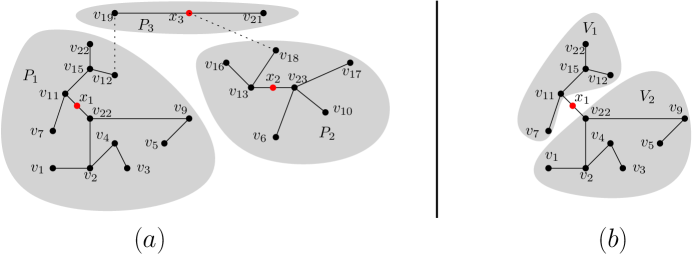
Figure 6: An example of a solution of the continuous version of the problem. In (a) the sinks $x_{1}$ and $x_{2}$ are on edges. (b) further decomposes $P_{1}$ to illustrate the fact that if a sink is on an edge $(u,v)$ then it has exactly two branches falling off of it.

For consistency, the oracle $\mathcal{A}$ extended to $x$ being on an edge must satisfy certain conditions. These are restated from [15] using the notation of this paper.

Definition 12.

(Fig. 7) Let $T=(V,E)$ be a tree and $f(\cdot,\,\cdot)$ be a minmax monotone cost function as defined at the beginning of Section 2

For $e=(u,v)\in E$, orient $e$ so that it starts at $u$ and ends at $v$. Let $V_{u}\subseteq V$ be a subtree of $T$ such that $u\in V_{u}$ but $v\not\in V_{u}$ and $x,x^{\prime}\in e$. Denote

$$x\leq x^{\prime} x u x^{\prime}$$ if and only if is on the path from to

$$x<x^{\prime} x\leq x^{\prime} x\not=x^{\prime}.$$ if and only if and

$f(\cdot,\cdot)$ is continuous if it satisfies:

1. $f(V_{u}\cup\{x\},x)$ is a continuous function in $\{x\,:\,u<x\leq v\}.$

2. $f(V_{u}\cup\{x\},x)$ is non-decreasing in $\{x\,:\,u\leq x\leq v\}$, i.e.,

   $$\forall u\leq x<x^{\prime}\leq v,\ f(V_{u}\cup\{x\},x)\leq f(V_{u}(u)\cup\{x^{\prime}\},x^{\prime}).$$

Point 2 is the natural generalization of path-monotonicity.

Figure 7: Let $(u,v)$ be oriented so that is starts at $u$ and ends at $v$. Then $x<x^{\prime}$. If the edge was oriented as ($v,u)$ then $x^{\prime}<x^{\prime}$ If $x\leq x^{\prime}$ then $f(V_{u}\cup\{x\},x)\leq f(V_{v}\cup\{x^{\prime}\},x^{\prime})$.

As noted in [15], $\Theta(\cdot,\,\cdot:s)$ will naturally satisfy these conditions. More specifically, let $d(x,v)$ denote the time required to travel from $x$ to $v$. It is natural to assume that this is a non-increasing continuous function in $x$ since flow travels smoothly without congestion inside an edge. If the last flow arrived at node $v$ at time $t$, then it had arrived at $x>u$ at time $t-d(x,v)$. Thus

$$\Theta(V_{u}\cup\{x\},x:s)=f(V_{u}\cup\{v\},v:s)-d(x,v),$$ (12)

so condition (1) is satisfied and condition (2) is satisfied for every $x$ except possibly $x=u.$ Now consider the time $t^{\prime}$ that the last flow arrives at node $u$ and let $t^{\prime}+w$ be the time that this last flow enters edge $(u,v)$. Since flow doesn’t encounter congestion inside an edge, it arrives at $v$ at time $t^{\prime}+w+d(u,v).$ Then

$$f(V_{u},u)=t^{\prime}\leq t^{\prime}+w=(t^{\prime}+w+d(u,v))-d(u,v)=\lim_{x\downarrow u}f(V_{u}\cup\{x\},x).$$

Thus condition (2) is also satisfied at $x=u.$ Note that $w>0$ only occurs if there is congestion at $(u,v)$ and this creates a left discontinuity, which is why the range in condition (1) does not include $x=u.$

Since conditions (1) and (2) hold for every $\Theta(\cdot,\,\cdot:s)$ they also hold for

$$r(V^{\prime},x)=\max_{s\in\mathcal{S}^{*}(V^{\prime},x)}\left\{\Theta(V^{\prime},x:s)-\Theta_{\rm OPT}(s)\right\}$$ (13)

and thus for $\bar{r}(V^{\prime},x)=\max(r(V^{\prime},x),\,0).$ That is, $\bar{r}(V^{\prime},x)$ is a contimuious minmax cost-function as defined by Definition 12.

Lemma 8 ([15]).

Let $T^{\prime}=(V^{\prime},E^{\prime})$ be a tree, $f(\cdot,\,\cdot)$ a continuous monotone min-max cost function and $e=(u,v)\in E.$ Let $V_{u}\subseteq V^{\prime}$ be a subtree of $T$ such that $u\in V_{u}$ but $v\not\in V_{u}$ and $V_{v}\subseteq V^{\prime}$ a subtree of $T$ such that $v\in V_{v}$ but $u\not\in V_{v}$.

Then both

$$s_{\mathcal{T}}=\max_{x\in e}\Bigl{(}f(V_{u}\cup\{x\},x)\leq\mathcal{T}\Bigr{)}$$ (14)

and

$$a:=\min_{x\in e}\max\Bigl{(}f(V_{u}\cup\{x\},x),f(V_{v}\cup\{x\},x)\Bigr{)}$$ (15)

exist.

Note: $s_{\mathcal{T}}$ and $a$ will be needed by the algorithm in [15] to find candidate sink locations.

Finally, restated in our notation, it was shown

Theorem 4 ([15]).

Let $f(\cdot,\,\cdot)$ be a continuous minmax monotone function with subadditive oracle $\mathcal{A}.$ Further suppose that $s_{\mathcal{T}}$ from Lemma 8 along with the largest $x^{\prime}\in e$ such that

$$s_{\mathcal{T}}=f(V_{u}\cup\{x^{\prime}\},x^{\prime})$$

can be calculated using $O(1)$ oracle calls using $O(t_{\mathcal{A}}(n_{1}))$ time, while $a$ and any $x^{\prime}\in e$ for which

$$a=\max\Bigl{(}f(V_{u}\cup\{x^{\prime}\},x^{\prime}),f(V_{v}\cup\{x^{\prime}\},x^{\prime})\Bigr{)}$$

can be calculated using $O(1)$ oracle calls using $O(t_{\mathcal{A}}(n_{1}+n_{2}))$ time where $n_{1}=|V_{u}|$ and $n_{2}=|V_{v}|.$ Then the continuous $k$-center partitioning problem on $T$ can be solved in time

$$O\bigl{(}\max(k,\log n)kt_{\mathcal{A}}(n)\log^{2}n\bigr{)}.$$

Note that if $x\in e$, then combining Eqs. 12 and 13 yields that

$$r(V_{u}\cup\{x\},x) = r(V_{u}\cup\{v\},v)-d(x,v)$$

$$r(V_{v}\cup\{x\},x) = r(V_{v}\cup\{u\},u)-d(u,x).$$

Thus $\bar{r}(\cdot,\,\cdot)$ satisfies the conditions of the Theorem 4. Similar to the discrete case, combining Theorem 4 with Lemma 7 immediately implies that that the minmax regret value can be calculated in

$$O\Bigl{(}\max(k,\log n)\,k^{2}\,t_{\mathcal{A}}(n)\,\log^{2}n\Bigr{)}=O\Bigl{(}\max(k^{2},\log^{2}n)\,k^{2}n^{2}\log^{5}n\Bigr{)}$$

time, completing the proof of Theorem 1 in the continuous case.

7 Conclusions and Extensions

This paper provided the first polynomial time algorithm for the Minmax-Regret $k$-Sink Location problem on a Dynamic Tree Network with uniform capacities and $k>1.$ It worked by noting (Section 5) that the minmax-regret function, which seems inherently global, can be expressed in terms of local minmax-regret functions and that (Section 4) each of these local min-max regret functions can be efficiently calculated. It then applied a tree-partitioning technique from [15] to these local regret functions to calculate the global minmax-regret

One obvious extension would be to try and extend this result to the Minmax-Regret $k$-Sink Location problem on a Dynamic Tree Network with general edge capacities. As noted in the introduction, absolutely no results seem to be known for this general problem, even restricted to paths and even for $k=1$. The structural reason for this is that, in the general capacity case, even though Section 4, the expression of the global cost in terms of local costs, would still hold, Section 5, the efficient calculation of these global costs, is not possible. More technically, the equivalent of Lemma 5 fails in the general capacity case in that it does not seem possible to restrict the set of worse case scenarios to a linear (or even polynomial) size set. Any extension of the approach in this paper to solving the general capacity problem would have to first confront that difficulty.

Another extension would be to try to utilize the approach developed here to apply to other minmax-regret functions. This is possible. As an example, consider the weighted $k$-center problem. This can be expressed using the minmax function on one tree defined by

$$f(V,x)=\max_{v\in V}w_{v}(s)d(x,v).$$

Note that this can be evaluated in $t_{\mathcal{A}}(|V|)=O(|V|)$ time instead of the $O(|V|\log|V|)$ required for sink evacuation. The weighted $k$-center problem is then to find a minimum-cost partition of the tree using this $f(\cdot,\,\cdot)$. The minmax-regret weighted $k$ center problem is then defined naturally.

It is straightforward to modify all of the results in the paper, including Lemma 5 and Section 5, to show that they all work for minmax-regret weighted $k$-center. Plugging in the oracle costs would yield a final running time of

$$O\Bigl{(}\max(k^{2},\log^{2}n)\,k^{2}n^{2}\log^{3}n\Bigr{)}.$$ (16)

This is not particularly useful though because [4] already gives a $O(n^{2}\log^{2}n\log\log n)$ time solution for the same problem. Working through the details, the intuitive reason that [4]’s algorithm is faster is because it strongly exploits the structural property that, in the $k$-center problem, the cost of a subtree only depends upon pairwise distances between points. In the sink-evacuation problem the cost of a subtree is dependent upon interactions between all of the nodes in the subtree, e.g., congestion effects, slowing down the partitioning time.

As a final observation we note that the techniques in this paper could solve restricted versions of the minmax-regret weighted $k$-center problem that [4]’s technique could not. As a simple example suppose that we artificially constrain the weighted $k$ center problem so that if center $x$ services node $v$ then all the nodes on the unique path from $x$ to $v$ must have weight at most $(w_{v}(s))^{2}.$ This would stop node weights from growing too rapidly along a path. This constraint corresponds to performing an optimal (min-cost) partitioning using the new minmax function

$$f(V,x)=\max_{v\in V}I(x,v).$$

where

$$I(x,v)=\left\{\begin{array}[]{ll}w_{v}(s)d(x,v)&\mbox{if all nodes $v^{\prime}$ on the path from $x$ to $v$ satisfy $w_{v^{\prime}}(s)\leq(w_{v}(s))^{2}.$}\\ \infty&\mbox{otherwise}\end{array}\right.$$

Note that this $f(V,x)$ can again be evaluated in in $t_{\mathcal{A}}(|V|)=O(|V|)$ time. The minmax-regret weighted $k$ center problem for these restricted partitions is then defined naturally. Exactly the same as above, plugging in the oracle cost would yield the same final running time as Eq. (16). As noted, this is only an artificial problem constructed to illustrate the power of the technique developed in this paper. We are not aware of any currently outstanding problems in the minmax-regret literature for which this paper’s technique can improve the running time.

References

- [1] Hassene Aissi, Cristina Bazgan, and Daniel Vanderpooten. Min–max and min–max regret versions of combinatorial optimization problems: A survey. European Journal of Operational Research, 197(2):427–438, 2009.
- [2] J. E. Aronson. A survey of dynamic network flows. Annals of Operations Research, 20(1):1–66, 1989.
- [3] Guru Prakash Arumugam, John Augustine, Mordecai J. Golin, and Prashanth Srikanthan. A polynomial time algorithm for minimax-regret evacuation on a dynamic path. CoRR, abs/1404.5448, 2014.
- [4] I. Averbakh and O. Berman. Minimax regret p-center location on a network with demand uncertainty. Location Science, 5(4):247–254, 1997.
- [5] Igor Averbakh and Vasilij Lebedev. Interval data minmax regret network optimization problems. Discrete Applied Mathematics, 138(3):289–301, 2004.
- [6] Binay Bhattacharya, Mordecai J. Golin, Yuya Higashikawa, Tsunehiko Kameda, and Naoki Katoh. Improved algorithms for computing k-sink on dynamic flow path networks. In Proceedings of WADS’2017, 2017.
- [7] Binay Bhattacharya and Tsunehiko Kameda. Improved algorithms for computing minmax regret sinks on dynamic path and tree networks. Theoretical Computer Science, 607:(411–425), 2015.
- [8] Binay Bhattacharya, Tsunehiko Kameda, and Zhao Song. A Linear Time Algorithm for Computing Minmax Regret 1-Median on a Tree Network. Algorithmica, pages 1–20, Nov 2013.
- [9] Binay Bhattacharya, Tsunehiko Kameda, and Zhao Song. Minmax regret 1-center algorithms for path/tree/unicycle/cactus networks. Discrete Applied Mathematics, pages 1–13, Nov 2014.
- [10] Binay K. Bhattacharya and Tsunehiko Kameda. A linear time algorithm for computing minmax regret 1-median on a tree. In COCOON’2012, pages 1–12, 2012.
- [11] Gerth Stølting Brodal, Loukas Georgiadis, and Irit Katriel. An O(nlogn) version of the Averbakh–Berman algorithm for the robust median of a tree. Operations Research Letters, 36(1):14–18, January 2008.
- [12] Alfredo Candia-Véjar, Eduardo Álvarez-Miranda, and Nelson Maculan. Minmax regret combinatorial optimization problems: an Algorithmic Perspective. RAIRO - Operations Research, 45(2):101–129, August 2011.
- [13] Danny Z. Chen, Jian Li, and Haitao Wang. Efficient algorithms for the one-dimensional k-center problem. Theoretical Computer Science, 592:135–142, 2015.
- [14] Di Chen and Mordecai Golin. Sink Evacuation on Trees with Dynamic Confluent Flows. In 27th International Symposium on Algorithms and Computation (ISAAC 2016), pages 25:1–25:13, 2016.
- [15] Di Chen and Mordecai J. Golin. Minmax centered k-partitioning of trees and applications to sink evacuation with dynamic confluent flows. CoRR, abs/1803.09289, 2014.
- [16] Jiangzhuo Chen, Robert D Kleinberg, László Lovász, Rajmohan Rajaraman, Ravi Sundaram, and Adrian Vetta. (Almost) Tight bounds and existence theorems for single-commodity confluent flows. Journal of the ACM, 54(4), jul 2007.
- [17] Jiangzhuo Chen, Rajmohan Rajaraman, and Ravi Sundaram. Meet and merge: Approximation algorithms for confluent flows. Journal of Computer and System Sciences, 72(3):468–489, 2006.
- [18] Siu-Wing Cheng, Yuya Higashikawa, Naoki Katoh, Guanqun Ni, Bing Su, and Yinfeng Xu. Minimax regret 1-sink location problems in dynamic path networks. In Proceedings of TAMC’2013, pages 121–132, 2013.
- [19] Eduardo Conde. A note on the minmax regret centdian location on trees. Operations Research Letters, 36(2):271–275, 2008.
- [20] Daniel Dressler and Martin Strehler. Capacitated Confluent Flows: Complexity and Algorithms. In 7th International Conference on Algorithms and Complexity (CIAC’10), pages 347–358, 2010.
- [21] Lisa Fleischer and Martin Skutella. Quickest Flows Over Time. SIAM Journal on Computing, 36(6):1600–1630, January 2007.
- [22] Lisa Fleischer and Éva Tardos. Efficient continuous-time dynamic network flow algorithms. Operations Research Letters, 23(3):71–80, 1998.
- [23] L. R. Ford and D. R. Fulkerson. Constructing Maximal Dynamic Flows from Static Flows. Operations Research, 6(3):419–433, June 1958.
- [24] Michael R Garey and David S Johnson. Computers and intractability: A Guide to the Theory of NP-Completeness. W.H. Freeman and Company, 1979.
- [25] Mordecai Golin, Hadi Khodabande, and Bo Qin. Non-approximability and polylogarithmic approximations of the single-sink unsplittable and confluent dynamic flow problems. In Proceedings of the 27th International Symposium on Algorithms and Computation (ISAAC’16), 2017.
- [26] Yuya Higashikawa. Studies on the Space Exploration and the Sink Location under Incomplete Information towards Applications to Evacuation Planning. PhD thesis, Kyoto University, 2014.
- [27] Yuya Higashikawa, John Augustine, Siu-Wing Cheng, Mordecai J. Golin, Naoki Katoh, Guanqun Ni, Bing Su, and Yinfeng Xu. Minimax regret 1-sink location problem in dynamic path networks. Theoretical Computer Science, 588(11):24–36, 2015.
- [28] Yuya Higashikawa, M. J. Golin, and Naoki Katoh. Minimax Regret Sink Location Problem in Dynamic Tree Networks with Uniform Capacity. In Proceedings of the 8’th International Workshop on Algorithms and Computation (WALCOM’2014), pages 125–137, 2014.
- [29] Yuya Higashikawa, Mordecai J Golin, and Naoki Katoh. Multiple Sink Location Problems in Dynamic Path Networks. In Proceedings of the 2014 International Conference on Algorithmic Aspects of Information and Management (AAIM 2014), 2014.
- [30] B Hoppe and É Tardos. The quickest transshipment problem. Mathematics of Operations Research, 25(1):36–62, 2000.
- [31] Naoyuki Kamiyama, Naoki Katoh, and Atsushi Takizawa. Theoretical and Practical Issues of Evacuation Planning in Urban Areas. In The Eighth Hellenic European Research on Computer Mathematics and its Applications Conference (HERCMA2007), pages 49–50, 2007.
- [32] Panos Kouvelis and Gang Yu. Robust Discrete Optimization and Its Applications. Kluwer Academic Publishers, 1997.
- [33] Hongmei Li, Yinfeng Xu, and Guanqun Ni. Minimax regret vertex 2-sink location problem in dynamic path networks. Journal of Combinatorial Optimization, February 2014.
- [34] Satoko Mamada, Takeaki Uno, Kazuhisa Makino, and Satoru Fujishige. An algorithm for the optimal sink location problem in dynamic tree networks. Discrete Applied Mathematics, 154(2387-2401):251–264, 2006.
- [35] Marta M. B. Pascoal, M. Eugénia V. Captivo, and João C. N. Clímaco. A comprehensive survey on the quickest path problem. Annals of Operations Research, 147(1):5–21, August 2006.
- [36] J. Puerto, A. M. Rodriguez-Chia, and A. Tamir. Minimax Regret Single-Facility Ordered Median Location Problems on Networks. INFORMS Journal on Computing, 21(1):77–87, August 2008.
- [37] Justo Puerto, Federica Ricca, and Andrea Scozzari. Minimax Regret Path Location on Trees. Networks, 58(2):147–158, 2011.
- [38] F. Bruce Shepherd and Adrian Vetta. The Inapproximability of Maximum Single-Sink Unsplittable, Priority and Confluent Flow Problems. arXiv:1504.0627, 2015.
- [39] Martin Skutella. An introduction to network flows over time. In William Cook, László Lovász, and Jens Vygen, editors, Research Trends in Combinatorial Optimization, pages 451–482. Springer, 2009.
- [40] Haitao Wang. Minmax Regret 1-Facility Location on Uncertain Path Networks. Proceedings of the 24th International Symposium on Algorithms and Computation (ISAAC’13), pages 733–743, 2013.
- [41] Haitao Wang. Minmax regret 1-facility location on uncertain path networks. European Journal of Operational Research, 239(3):636–643, 2014.
- [42] Yinfeng Xu and Hongmei Li. Minimax regret 1-sink location problem in dynamic cycle networks. Information Processing Letters, 115(2):163–169, 2015.
- [43] Jhih-Hong Ye and Biing-Feng Wang. On the minmax regret path median problem on trees. Journal of Computer and System Sciences, 1:1–12, 2015.
- [44] Hung-I. Yu, Tzu-Chin Lin, and Biing-Feng Wang. Improved algorithms for the minmax-regret 1-center and 1-median problems. ACM Transactions on Algorithms, 4(3):1–27, June 2008.