Distributed Kalman Filter for A Class of Nonlinear Uncertain Systems: An Extended State Method

Abstract

This paper studies the distributed state estimation problem for a class of discrete-time stochastic systems with nonlinear uncertain dynamics over time-varying topologies of sensor networks. An extended state vector consisting of the original state and the nonlinear dynamics is constructed. By analyzing the extended system, we provide a design method for the filtering gain and fusion matrices, leading to the extended state distributed Kalman filter. It is shown that the proposed filter can provide the upper bound of estimation covariance in real time, which means the estimation accuracy can be evaluated online. It is proven that the estimation covariance of the filter is bounded under rather mild assumptions, i.e., collective observability of the system and jointly strong connectedness of network topologies. Numerical simulation shows the effectiveness of the proposed filter.

I Introduction

In recent years, networked state estimation problems are drawing more and more attention of researchers, due to the broad applications in environmental monitoring, target tracking over networks, collaborative information processing, etc. Two main strategies, namely, the centralized and the distributed, have been considered to deal with the state estimation problems over networks. The Kalman filter based fusion estimation problems were studied in [1, 2], where each sensor can fuse the information from all the other sensors over the network to obtain the better estimate. In the distributed strategy, the communications between sensors follow a peer-to-peer protocol. Compared with the centralized strategy, the distributed one has shown more robustness in network structure, better performance in energy saving and stronger ability in parallel processing.

In the existing literature on distributed state estimation, many effective methods and some theoretical analysis tools have been provided. A distributed estimator with time-invariant filtering gain was studied in [3], where the relationship between the instability of system and the boundedness of estimation error was evaluated. A distributed Kalman filter (DKF) based on measurement consensus strategy was proposed in [4], where the design method of the consensus weights and the filtering gain were investigated. In [5], a diffusion DKF with constant weights was studied and the performance of the proposed filter was analyzed theoretically. Yet, the results were based on a local observability condition , which is difficult to be met in a large network. Besides, there were many methods and results related to the distributed state estimation. Interested readers can refer to [6, 7, 8, 9] and the references therein.

The state estimation problems for nonlinear systems have been studied for a few decades. Through linearizing the nonlinear system to the first order, the extended Kalman filter (EKF) was constructed in the form of Kalman filter [10] to achieve the state estimation and prediction. Based on the third-order linearization for any known nonlinearity, unscented Kalman filter (UKF) can accurately achieve the estimation on the posterior mean and covariance [11]. For the nonlinear uncertain systems, quite a few robust filters including $H_{\infty}$ filters and set valued filters have been studied by many researchers [12, 13, 14]. The essential idea was to minimize a worst-case bound so as to obtain a conservative estimate of the state under deterministic or stochastic uncertainties of the system. Due to the instability issue of the linearization methods and the conservativeness of the robust filters, [15] proposed an extended state Kalman filter to handle the state estimation for a class of nonlinear time-varying uncertain systems. Moreover, the upper boundedness of the estimation covariance and the optimality of estimation in some certain conditions are discussed. The corresponding continuous-time problem was studied in [16], which proposed an extended state Kalman-Bucy filter and analyzed the main performance of the filter. While, all the above filters still face many problems when they are utilized to the sensor networks, especially in the aspects of stability analysis and performance evaluation. Thus, more attention should be paid to the research of distributed state estimation for nonlinear uncertain systems.

In this paper, we study the distributed state estimation for a class of discrete-time stochastic systems with nonlinear uncertain dynamics over time-varying topologies of sensor networks. The main contributions of this paper are summarized. First, a new extended state method is provided and the method can achieve the simultaneous estimation of the original state and the nonlinear dynamics. By designing adaptive fusion matrices and filtering gain, the upper bounds of estimation covariances can be obtained in real time. Second, it is proven that the estimation covariance of the filter is bounded under rather mild assumptions, i.e., collective observability of system and jointly strong connectedness of network topologies.

The remainder of the paper is organized as follows: Section II is on the preliminaries and problem formulation. Section III presents the main results of this paper. Section IV shows the numerical simulation. The conclusion of this paper is given in Section V. Due to the limitation of the pages, the proofs are omitted. Interested readers can refer to the full version in [17] for the detailed proofs.

I-A Notations

The superscript “T” represents the transpose. $I_{n}$ stands for the identity matrix with $n$ rows and $n$ columns. $E\{x\}$ denotes the mathematical expectation of the stochastic variable $x$, and $blockdiag\{\cdot\}$ means the block elements are arranged in diagonals. $diag\{\cdot\}$ represent the diagonalization scalar elements. $tr(P)$ is the trace of the matrix $P$. $\mathbb{N}^{+}$ denotes the set of positive natural numbers. $\mathbb{R}^{n}$ stands for the set of $n$-dimensional real vectors.

II Preliminaries and Problem Formulation

II-A Preliminaries in Graph Theory

Let $\mathcal{G}=(\mathcal{V},\mathcal{E}_{\mathcal{G}},\mathcal{A}_{\mathcal{G}})$ be a weighted digraph, which consists of the node set $\mathcal{V}=\{1,2,\cdots,N\}$, the set of edges $\mathcal{E}_{\mathcal{G}}\subseteq\mathcal{V}\times\mathcal{V}$ and the weighted adjacent matrix $\mathcal{A}_{\mathcal{G}}=[a_{i,j}]\in\mathbb{R}^{N\times N}$. In the weighted adjacent matrix $\mathcal{A}_{\mathcal{G}}$, all the elements are nonnegative, row stochastic and the diagonal elements are all positive, i.e., $a_{i,i}>0,a_{i,j}\geq 0,\sum_{j\in\mathcal{V}}a_{i,j}=1$. If $a_{i,j}>0,j\neq i$, there is a link $(i,j)\in\mathcal{E}_{\mathcal{G}}$, which means node $i$ can directly receive the information of node $j$ through the communication channel. In this situation, node $j$ is called the neighbor of node $i$ and all the neighbors of node $i$ including itself can be represented by the set $\{j\in\mathcal{V}|(i,j)\in\mathcal{E}_{\mathcal{G}}\}\bigcup\{i\}\triangleq\mathcal{N}_{i}^{\mathcal{G}}$, whose size is denoted as $|\mathcal{N}_{i}^{\mathcal{G}}|$. For a given positive integer $L$, the union of the $L$ digraphs $\mathcal{G}_{1}=(\mathcal{V},\mathcal{E}_{\mathcal{G}_{1}},\mathcal{A}_{\mathcal{G}_{1}}),\cdots,\mathcal{G}_{L}=(\mathcal{V},\mathcal{E}_{\mathcal{G}_{L}},\mathcal{A}_{\mathcal{G}_{L}})$ is denoted as $\sum_{l=1}^{L}\mathcal{G}_{l}=(\mathcal{V},\sum_{l=1}^{L}\mathcal{E}_{\mathcal{G}_{l}},\sum_{l=1}^{L}\mathcal{A}_{\mathcal{G}_{l}})$. $\mathcal{G}$ is called strongly connected if for any pair nodes $(i_{1},i_{l})$, there exists a direct path from $i_{1}$ to $i_{l}$ consisting of edges $(i_{1},i_{2}),(i_{2},i_{3}),\cdots,(i_{l-1},i_{l})$. We call $\{\mathcal{G}_{1},\cdots,\mathcal{G}_{L}\}$ jointly strongly connected if $\sum_{l=1}^{L}\mathcal{G}_{l}$ is strongly connected.

II-B Problem Formulation

Consider the following discrete-time stochastic system

$$\begin{cases}x_{k+1}=\bar{A}_{k}x_{k}+\bar{G}_{k}F(x_{k},k)+\bar{\omega}_{k},\\ y_{k,i}=\bar{H}_{k,i}x_{k}+v_{k,i},i=1,2,\cdots,N,\end{cases}$$ (1)

where $x_{k}$ is the unknown $n$-dimensional system state, $\bar{A}_{k}$ is the known system matrix and $\bar{\omega}_{k}$ is the zero-mean unknown process noise with $E\{\bar{\omega}_{k}\bar{\omega}_{k}^{T}\}>0$. $F(x_{k},k)$ is the $p$-dimensional uncertain dynamics consisting of the known nominal model $\bar{F}(x_{k},k)$ and some unknown disturbance. For convenience, we define $F(x_{k},k)\triangleq F_{k}$ and $\bar{F}(x_{k},k)\triangleq\bar{F}_{k}$. $N$ is the number of sensors over the network. $y_{k,i}$ is the $m_{i}$-dimensional measurement vector obtained via sensor $i$, $\bar{H}_{k,i}$ is the known measurement matrix, and $v_{k,i}$ is the zero-mean stochastic measurement noise. $\{\bar{\omega}_{k}\}_{k=0}^{\infty}$, $\{v_{k,i}\}_{k=0}^{\infty}$ are independent of each other, and also independent of $x_{0}$ and $F_{0}$. It is noted that $\bar{A}_{k}$, $\bar{G}_{k}$, $\bar{H}_{k,i}$, and $y_{k,i}$ are simply known to sensor $i$. The above matrices and vectors have compatible dimensions.

For the system (1), a new state vector, consisting of the original state $x_{k}$ and the nonlinear uncertain dynamics $F_{k}$, can be constructed. Then a modified system model with respect to the new state vector is given in the following.

$$\begin{cases}\begin{pmatrix}x_{k+1}\\ F_{k+1}\end{pmatrix}=\begin{pmatrix}\bar{A}_{k}&\bar{G}_{k}\\ 0&I_{p}\end{pmatrix}\begin{pmatrix}x_{k}\\ F_{k}\end{pmatrix}+\begin{pmatrix}\bar{\omega}_{k}\\ 0\end{pmatrix}\\ \qquad\qquad\qquad+\begin{pmatrix}0\\ I_{p}\end{pmatrix}(F_{k+1}-F_{k}),\\ y_{k,i}=\begin{pmatrix}\bar{H}_{k,i}&0\end{pmatrix}\begin{pmatrix}x_{k}\\ F_{k}\end{pmatrix}+v_{k,i}.\end{cases}$$ (2)

Define

$$\begin{cases}\begin{pmatrix}x_{k}\\ F_{k}\end{pmatrix}\triangleq X_{k},\begin{pmatrix}\bar{A}_{k}&\bar{G}_{k}\\ 0&I_{p}\end{pmatrix}\triangleq A_{k},\\ \begin{pmatrix}\bar{\omega}_{k}\\ 0\end{pmatrix}\triangleq\omega_{k},\begin{pmatrix}0\\ I_{p}\end{pmatrix}\triangleq D,\\ F_{k+1}-F_{k}\triangleq u_{k},\\ \begin{pmatrix}\bar{H}_{k,i}&0\end{pmatrix}\triangleq H_{k,i},\end{cases}$$ (3)

then the system (2) can be rewritten as

$$\begin{cases}X_{k+1}=A_{k}X_{k}+Du_{k}+\omega_{k},\\ y_{k,i}=H_{k,i}X_{k}+v_{k,i}.\end{cases}$$ (4)

In this paper, the following assumptions are needed.

Assumption 1.

The system (4) satisfies the following conditions

$$\begin{split}&E\{\omega_{k}\omega_{k}^{T}\}\leq Q_{k},\\ &E\{v_{k,i}v_{k,i}^{T}\}\leq R_{k,i},i=1,2,\cdots,N,\\ \ &E\{u_{k}^{2}(j)\}\leq q_{k}(j),j=1,2,\cdots,p,\end{split}$$ (5)

where $R_{k,i}>0$ and $q_{k}(j)>0$. Also, $Q_{k}$ and $q_{k}(j)$ are uniformly upper bounded.

The noise conditions given in Assumption 1 are reasonable and easy to be satisfied due to the power limitation of practical systems. Different from the result [18] that treats the uncertain dynamics as a bounded total disturbance, the requirement for the increment of the nonlinear dynamics in Assumption 1 poses no restriction on the boundedness of uncertain dynamics. It is a mild condition for the systems with nonlinear uncertain dynamics.

Assumption 2.

There exists a positive integer $\bar{N}$ and a constant $\alpha>0$ such that for any $k\geq 0$, there is

$$\sum_{i=1}^{N}\left[\sum_{j=k}^{k+\bar{N}}\Phi^{T}_{j,k}H_{j,i}^{T}R_{j,i}^{-1}H_{j,i}\Phi_{j,k}\right]\geq\alpha I_{n},$$ (6)

where

$$\Phi_{k,k}=I_{n},\Phi_{k+1,k}=A_{k},\Phi_{j,k}=\Phi_{j,j-1}\cdots\Phi_{k+1,k}(j>k).$$

Assumption 2 is a general collective observability condition [7], which is a desired condition to guarantee the stability of distributed estimation algorithms. If the system is time-invariant, then Assumption 2 degenerates to $(A,H)$ being observable [19, 20]. Besides, if the local observability condition of an individual sensor is satisfied [5], then Assumption 2 holds, but not vice versa.

In this paper, the topologies of the networks are assumed to be time-varying digraphs $\{\mathcal{G}_{\sigma_{k}},k\in\mathbb{N}^{+}\}$. $\sigma_{k}$ is the graph switching signal defined $\sigma_{k}:\mathbb{N}^{+}\rightarrow\Omega$, where $\Omega$ is the set of the underlying network topology numbers. For convenience, the weighted adjacent matrix of the digraph $\mathcal{G}_{\sigma_{k}}$ is denoted as $\mathcal{A}_{\sigma_{k}}=[a_{i,j}(k)]\in\mathbb{R}^{N\times N}$. To analyze the time-varying topologies, we consider the infinity interval sequence of bounded, non-overlapping and contiguous time intervals $[k_{l},k_{l+1}),l=0,1,\cdots,$ with $k_{0}=0$ and $0\leq k_{l+1}-k_{l}\leq k^{0}$ for some integer $k^{0}$. On the time-varying topologies of the networks, the following assumption is in need.

Assumption 3.

The digraph set $\{\mathcal{G}_{\sigma_{k}},k\in[k_{l},k_{l+1})\}$ is jointly strongly connected across the time interval $[k_{l},k_{l+1})$ and $a_{i,j}(k)\in\bar{\varPsi}$, $k\in\mathbb{N}^{+}$, where $\bar{\varPsi}$ is a finite set of arbitrary nonnegative numbers.

Assumption 3 is on the conditions of the network topologies. Since the jointly connectedness of the time-varying digraphs admits the network is unconnected at each moment, it is quite general for the networks facing with the link failures. If the network remains connected at each moment or fixed [19, 7], then Assumption 3 holds.

The objective of this paper is to estimate the extended state $X_{k}$ consisting of the original system state $x_{k}$ and the nonlinear dynamics $F_{k}$. To achieve the objective, a distributed filter is aimed to be designed for each sensor based on the information of the sensor and its neighbors.

III Main results

In this section, we will propose a distributed filtering structure and study the design methods for the structure, so as to raise the extended state distributed Kalman filter of this paper. Besides, we will study the performance of this filter in terms of the boundedness of estimation covariance.

In this paper, we consider the following distributed filter structure for sensor $i$, $\forall i\in\mathcal{V}$,

$$\begin{cases}\bar{X}_{k,i}=A_{k-1}\hat{X}_{k-1,i}+D\hat{u}_{k-1},\\ \tilde{X}_{k,i}=\bar{X}_{k,i}+K_{k,i}(y_{k,i}-H_{k,i}\bar{X}_{k,i}),\\ \hat{X}_{k,i}=\sum_{j\in\mathcal{N}_{i}}W_{k,i,j}\tilde{X}_{k,j},\end{cases}$$ (7)

where $\bar{X}_{k,i}$, $\tilde{X}_{k,i}$ and $\hat{X}_{k,i}$ are the extended state prediction, update and estimate of sensor $i$ at the $k$th moment, respectively. $K_{k,i}$ is the filtering gain matrix and $W_{k,i,j},j\in\mathcal{N}_{i}$, are the local fusion matrices. Additionally,

$$\begin{split}&\hat{u}_{k-1}(j)=sat\big{(}\hat{\bar{u}}_{k-1}(j),\sqrt{q_{k-1}(j)}\big{)},j=1,2,\cdots,p\\ &\hat{\bar{u}}_{k-1}=\bar{F}(\bar{A}_{k-1}\hat{x}_{k-1}+\bar{G}_{k-1}\hat{F}_{k-1},k)-\bar{F}(\hat{x}_{k-1},k-1)\end{split}$$ (8)

where $sat(\cdot)$ is the saturation function defined $sat(f,b)=\max\{\min{f,b},-b\},b>0$. It is noted that the saturation function is utilized to guarantee the boundedness of $\hat{u}_{k-1}$.

In the Kalman filter, the matrix $P_{k}$ stands for the estimation covariance, which can be recursively calculated. For the distributed Kalman filters, the estimation covariances are usually unaccessible, thus the following definition on consistency is introduced.

Definition 1.

([21]) Suppose $x_{k}$ is a random vector. Let $\hat{x}_{k}$ and $P_{k}$ be the estimate of $x_{k}$ and the estimate of the corresponding error covariance matrix. Then the pair ($\hat{x}_{k},P_{k}$) is said to be consistent (or of consistency) at the $k$th moment if

$$E\{(\hat{x}_{k}-x_{k})(\hat{x}_{k}-x_{k})^{T}\}\leq P_{k}.$$

Regarding the filtering structure (7), the condition for the initial estimation of each sensor is given in Assumption 4.

Assumption 4.

The initial estimation of each sensor is consistent, i.e.,

$$E\{(X_{0}-\hat{X}_{0,i})(X_{0}-\hat{X}_{0,i})^{T}\}\leq P_{0,i},$$ (9)

where $P_{0,i}>0,i\in\mathcal{V}$.

It is noted that Assumption 4 is quite general and easy to be met, since a sufficient large $P_{0,i}$ can always be set. Based on the filtering structure (7), Theorem 1 provides a design method of fusion matrices, which can lead to the consistent estimation of each sensor.

Theorem 1.

Under Assumptions 1 and 4, for $i\in\mathcal{V},\forall\theta>0$, it follows that

$$\begin{cases}E\{(\bar{X}_{k,i}-X_{k})(\bar{X}_{k,i}-X_{k})^{T}\}\leq\bar{P}_{k,i},\\ E\{(\tilde{X}_{k,i}-X_{k})(\tilde{X}_{k,i}-X_{k})^{T}\}\leq\tilde{P}_{k,i},\\ E\{(\hat{X}_{k,i}-X_{k})(\hat{X}_{k,i}-X_{k})^{T}\}\leq P_{k,i},\end{cases}$$ (10)

if $W_{k,i,j}$ in the filter structure (7) are designed with

$$\begin{split}W_{k,i,j}=a_{i,j}(k)P_{k,i}^{-1}\tilde{P}_{k,j}^{-1},\end{split}$$ (11)

then the pairs ($\bar{X}_{k,i},\bar{P}_{k,i}$),($\tilde{X}_{k,i},\tilde{P}_{k,i}$) and ($\hat{X}_{k,i},P_{k,i}$) are all consistent, where $\bar{P}_{k,i},\tilde{P}_{k,i}$ and $P_{k,i}$ evolve according to the following recursive forms:

$$\begin{split}&\bar{P}_{k,i}=(1+\theta)A_{k-1}P_{k-1,i}A_{k-1}^{T}+\frac{1+\theta}{\theta}\bar{Q}_{k-1}+Q_{k-1},\\ &\bar{Q}_{k-1}=4pD\cdot diag\{q_{k-1}(1),\dots,q_{k-1}(p)\}D^{T},\\ &\tilde{P}_{k,i}=(I-K_{k,i}H_{k,i})\bar{P}_{k,i}(I-K_{k,i}H_{k,i})^{T}+K_{k,i}R_{k,i}K_{k,i}^{T},\\ &P_{k,i}=\bigg{(}\sum_{j\in\mathcal{N}_{i}}a_{i,j}(k)\tilde{P}_{k,j}^{-1}\bigg{)}^{-1}.\end{split}$$ (12)

For the filtering gain matrix $K_{k,i}$, its design can be casted into an optimization problem given in the following lemma.

Lemma 1.

The solution of the optimization problem

$$\min_{K_{k,i}}\tilde{P}_{k,i}$$ (13)

in the sense of positive definiteness is

$$\begin{split}&K_{k,i}=\bar{P}_{k,i}H_{k,i}^{T}(H_{k,i}\bar{P}_{k,i}H_{k,i}^{T}+R_{k,i})^{-1}.\end{split}$$ (14)

In Theorem 1, it is shown that the upper bounds of estimation error covariances at three typical steps can be iteratively obtained by each sensor. The bounds can not only contribute to the design of fusion weights and filtering gain, but also be used to evaluate the estimation accuracy in real time.

Summing up the results of Theorem 1 and Lemma 1, the extended state distributed Kalman filter (ESDKF) is provided in Table I. In the next, we will study the boundedness of the estimation error covariance of each sensor under given conditions.

TABLE I: Extended State Distributed Kalman Filter (ESDKF):

Prediction:

$\bar{X}_{k,i}=A_{k-1}\hat{X}_{k-1,i}+D\hat{u}_{k-1},$

$\bar{P}_{k,i}=(1+\theta)A_{k-1}P_{k-1,i}A_{k-1}^{T}+\frac{1+\theta}{\theta}\bar{Q}_{k-1}+Q_{k-1},\forall\theta>0,$

where $\hat{u}_{k-1}$ and $\bar{Q}_{k-1}$ are given in (8) and (12), respectively.

Measurement Update:

$\tilde{X}_{k,i}=\bar{X}_{k,i}+K_{k,i}(y_{k,i}-H_{k,i}\bar{X}_{k,i})$

$K_{k,i}=\bar{P}_{k,i}H_{k,i}^{T}(H_{k,i}\bar{P}_{k,i}H_{k,i}^{T}+R_{k,i})^{-1}$

$\tilde{P}_{k,i}=(I-K_{k,i}H_{k,i})\bar{P}_{k,i}$,

Local Fusion: Receiving ($\tilde{X}_{k,j}$, $\tilde{P}_{k,j}$ ) from neighbors $j\in\mathcal{N}_{i}$

$\hat{X}_{k,i}=P_{k,i}\sum_{j\in\mathcal{N}_{i}}a_{i,j}(k)\tilde{P}_{k,j}^{-1}\tilde{X}_{k,j}$,

$P_{k,i}=\bigg{(}\sum_{j\in\mathcal{N}_{i}}a_{i,j}(k)\tilde{P}_{k,j}^{-1}\bigg{)}^{-1}$。

Theorem 2.

Under Assumptions 1-4 and the condition that $\{A_{k},k\in\mathbb{N}^{+}\}$ belongs to a nonsingular compact set, then there exists a positive definite matrix $\hat{P}$, such that

$$E\{(\hat{X}_{k,i}-X_{k})(\hat{X}_{k,i}-X_{k})^{T}\}\leq P_{k,i}\leq\hat{P},\forall i\in\mathcal{V}.$$ (15)

Through Theorem 2, it can be seen that, under mild conditions including collective observability of system and jointly strong connectedness of network topologies, the proposed filter can effectively estimate the extended state, consisting of the original state and the nonlinear dynamics.

IV Numerical Simulation

In this section, we will carry out a numerical simulation to show the effectiveness of the proposed filter. Consider the following fourth-order time-varying system with four sensors

$$\left\{\begin{aligned} x_{k+1}&=\begin{pmatrix}1&0&0.1&0\\ 0&1&0&0.1\\ 0&0&1&0\\ 0&0&0&1\end{pmatrix}x_{k}+\frac{1}{3}\begin{pmatrix}0\\ 0\\ \sin\left(x_{k}\left(3\right)\right)+k\\ \sin\left(x_{k}\left(4\right)\right)+k\end{pmatrix}\\ &\qquad+\omega_{k}\\ y_{k,i}&=\bar{H}_{k,i}x_{k}+v_{k,i},i=1,2,3,4\end{aligned}\right.,$$

where $x_{k}\in\mathrm{R}^{4}$ is the process and the observation matrices are

$$\left\{\begin{aligned} \bar{H}_{k,1}&=\begin{pmatrix}1&0&0&0\end{pmatrix}\\ \bar{H}_{k,2}&=\begin{pmatrix}0&1&0&0\end{pmatrix}\\ \bar{H}_{k,3}&=\begin{pmatrix}1&1&0&0\end{pmatrix}\\ \bar{H}_{k,4}&=\begin{pmatrix}0&0&0&0\end{pmatrix}\\ \end{aligned}\right..$$

Additionally, the network communication topologies, assumed as directed and time-varying, are illustrated in Fig. 1 with adjacent matrix selected from

$$\left\{\begin{aligned} \mathcal{A}_{1}&=\begin{pmatrix}1&0&0&0\\ 0.5&0.5&0&0\\ 0&0.5&0.5&0\\ 0&0&0.5&0.5\end{pmatrix}\\ \mathcal{A}_{2}&=\begin{pmatrix}0.5&0.5&0&0\\ 0&1&0&0\\ 0&0.3&0.4&0.3\\ 0&0.5&0&0.5\end{pmatrix}\\ \mathcal{A}_{3}&=\begin{pmatrix}0.5&0.5&0&0\\ 0&0.5&0.5&0\\ 0&0&1&0\\ 0.25&0.25&0.25&0.25\end{pmatrix}\\ \end{aligned}\right..$$

And the gragh switching signal $\sigma_{k}$ is

$$\left\{\begin{aligned} \sigma_{k}&=1,k=1:5,16:20,\cdots\\ \sigma_{k}&=2,k=6:10,21:25,\cdots\\ \sigma_{k}&=3,k=11:15,26:30,\cdots\end{aligned}\right..$$

(a) Topology 1

(b) Topology 2

(c) Topology 3

Figure 1: The topologies of sensor networks

Here, it is assumed that the process noise covariance matrix $Q=diag\{4,4,1,1\}$, and the whole measurement noise covariance matrix $R=diag\{90,90,90,90\}$, and the parameter $\theta=0.1$. The initial value has zero mean and covariance matrix being $100I_{4}$, and the initial estimation setting is $\hat{X}_{i,0}=0$ and $P_{i,0}=100I_{4},\forall i=1,2,3,4$. Next, we conduct the numerical simulation through Monte Carlo experiment, in which 500 runs for the proposed algorithm are implemented. The average performance function is defined $MSE_{k}=\frac{1}{4}\sum_{i=1}^{4}{MSE_{k,i}}$, where

$$MSE_{k,i}=\frac{1}{500}\sum_{j=1}^{500}{\left(X_{k,i}^{j}-\hat{X}_{k,i}^{j}\right)^{T}\left(X_{k,i}^{j}-\hat{X}_{k,i}^{j}\right)},$$

and $\hat{X}_{k,i}^{j}$ is the extended state estimate of the $j$th run of sensor $i$ at the $k$th moment. Besides, we define $P_{k}=\frac{1}{4}\sum_{i=1}^{4}{P_{k,i}}$.

The simulation results based on above parameter setting are gived in Fig. 2 and Fig. 3.

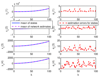
Figure 2: Tracking performance of ESDKF

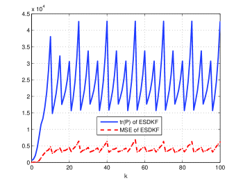
Figure 3: Performance evaluation of ESDKF

Fig. 2 shows the tracking performance for the system states and the estimation errors, from which one can see the algorithm can effectively estimate the overall state in the sense of mean value. The comparison between $MSE_{k,i}$ and $tr(P_{k,i})$ is depicted in Fig. 3, where it can be seen that the estimation errors of the proposed algorithm keep stable in the given period and the consistency of each sensor remains.

V Conclusion

In this paper, the distributed state estimation problem was studied for a class of discrete-time stochastic systems with nonlinear uncertain dynamics over time-varying topologies. Through extending the original state and the nonlinear dynamics to a new state vector, an extended system was constructed. Then, a design method for the filtering gain and fusion matrices was proposed. It was shown that the proposed filter was consistent, i.e., the upper bound of estimation covariance can be provided in real time. It was proven that the estimation covariance of the filter was bounded under rather mild assumptions, i.e., collective observability of the system and jointly strong connectedness of network topologies. Through numerical simulations, the effectiveness of the distributed filter was testified.

References

• [1] F.ย Pfaff, B.ย Noack, U.ย D. Hanebeck, F.ย Govaers, and W.ย Koch, โ€œInformation form distributed Kalman filtering with explicit inputs,โ€ in International Conference on Information Fusion, pp.ย 1โ€“8, 2017.
• [2] C.ย Y. Chong, S.ย Mori, F.ย Govaers, and W.ย Koch, โ€œComparison of tracklet fusion and distributed Kalman filter for track fusion,โ€ in International Conference on Information Fusion, 2014.
• [3] U.ย A. Khan and A.ย Jadbabaie, โ€œCollaborative scalar-gain estimators for potentially unstable social dynamics with limited communication,โ€ Automatica, vol.ย 50, no.ย 7, pp.ย 1909โ€“1914, 2014.
• [4] S.ย Das and J.ย M.ย F. Moura, โ€œDistributed Kalman filtering with dynamic observations consensus,โ€ IEEE Transactions on Signal Processing, vol.ย 63, no.ย 17, pp.ย 4458โ€“4473, 2015.
• [5] F.ย S. Cattivelli and A.ย H. Sayed, โ€œDiffusion strategies for distributed Kalman filtering and smoothing,โ€ IEEE Transactions on Automatic Control, vol.ย 55, no.ย 9, pp.ย 2069โ€“2084, 2010.
• [6] M.ย S. Mahmoud and H.ย M. Khalid, โ€œDistributed Kalman filtering: a bibliographic review,โ€ IET Control Theory & Applications, vol.ย 7, no.ย 4, pp.ย 483โ€“501, 2013.
• [7] X.ย He, W.ย Xue, and H.ย Fang, โ€œConsistent distributed state estimation with global observability over sensor network,โ€ Automatica, vol.ย 92, pp.ย 162โ€“172, 2018.
• [8] G.ย Battistelli, L.ย Chisci, G.ย Mugnai, A.ย Farina, and A.ย Graziano, โ€œConsensus-based linear and nonlinear filtering,โ€ IEEE Transactions on Automatic Control, vol.ย 60, no.ย 5, pp.ย 1410โ€“1415, 2015.
• [9] W.ย Yang, C.ย Yang, H.ย Shi, L.ย Shi, and G.ย Chen, โ€œStochastic link activation for distributed filtering under sensor power constraint,โ€ Automatica, vol.ย 75, pp.ย 109โ€“118, 2017.
• [10] K.ย Reif, S.ย Gunther, E.ย Yaz, and R.ย Unbehauen, โ€œStochastic stability of the discrete-time extended Kalman filter,โ€ IEEE Transactions on Automatic Control, vol.ย 44, no.ย 4, pp.ย 714โ€“728, 1999.
• [11] S.ย J. Julier and J.ย K. Uhlmann, โ€œUnscented filtering and nonlinear estimation,โ€ Proceedings of the IEEE, vol.ย 92, no.ย 3, pp.ย 401โ€“422, 2004.
• [12] G.ย Yang and W.ย Che, โ€œNon-fragile ${H}_{\infty}$ filter design for linear continuous-time systems,โ€ Automatica, vol.ย 44, no.ย 11, pp.ย 2849โ€“2856, 2008.
• [13] D.ย Ding, Z.ย Wang, H.ย Dong, and H.ย Shu, โ€œDistributed ${H}_{\infty}$ state estimation with stochastic parameters and nonlinearities through sensor networks: the finite-horizon case,โ€ Automatica, vol.ย 48, no.ย 8, pp.ย 1575โ€“1585, 2012.
• [14] G.ย Calafiore, โ€œReliable localization using set-valued nonlinear filters,โ€ IEEE Transactions on systems, man, and cybernetics-part A: systems and humans, vol.ย 35, no.ย 2, pp.ย 189โ€“197, 2005.
• [15] W.ย Bai, W.ย Xue, Y.ย Huang, and H.ย Fang, โ€œOn extended state based Kalman filter design for a class of nonlinear time-varying uncertain systems,โ€ Science China Information Sciences, vol.ย 61, no.ย 4, p.ย 042201, 2018.
• [16] X.ย Zhang, W.ย Xue, H.ย Fang, and X.ย He, โ€œOn extended state based Kalman-Bucy filter,โ€ in IEEE 7th Data Driven Control and Learning Systems Conference, 2018.
• [17] X.ย He, X.ย Zhang, W.ย Xue, and H.ย Fang, โ€œDistributed Kalman filter for a class of nonlinear uncertain systems: An extended state method,โ€ DOI: 10.13140/RG.2.2.34429.26088, 2018.
• [18] Z.ย Cai, M.ย S.ย D. Queiroz, and D.ย M. Dawson, โ€œRobust adaptive asymptotic tracking of nonlinear systems with additive disturbance,โ€ IEEE Transactions on Automatic Control, vol.ย 51, no.ย 3, pp.ย 524โ€“529, 2006.
• [19] G.ย Battistelli and L.ย Chisci, โ€œKullback-Leibler average, consensus on probability densities, and distributed state estimation with guaranteed stability,โ€ Automatica, vol.ย 50, no.ย 3, pp.ย 707โ€“718, 2014.
• [20] X.ย He, C.ย Hu, W.ย Xue, and H.ย Fang, โ€œOn event-based distributed Kalman filter with information matrix triggers,โ€ in IFAC World Congress, pp.ย 14873โ€“14878, 2017.
• [21] S.ย J. Julier and J.ย K. Uhlmann, โ€œA non-divergent estimation algorithm in the presence of unknown correlations,โ€ in Proceedings of the American Control Conference, pp.ย 2369โ€“2373, 1997.