The $\phi^{4}$ Model, Chaos, Thermodynamics, and the
2018 SNOOK Prizes in Computational Statistical Mechanics

Abstract

The one-dimensional $\phi^{4}$ Model generalizes a harmonic chain with nearest-neighbor Hooke’s-Law interactions by adding quartic potentials tethering each particle to its lattice site. In their studies of this model Kenichiro Aoki and Dimitri Kusnezov emphasized its most interesting feature : because the quartic tethers act to scatter long-wavelength phonons, $\phi^{4}$ chains exhibit Fourier heat conduction. In his recent Snook-Prize work Aoki also showed that the model can exhibit chaos on the three-dimensional energy surface describing a two-body two-spring chain. That surface can include at least two distinct chaotic seas. Aoki pointed out that the model typically exhibits different kinetic temperatures for the two bodies. Evidently few-body $\phi^{4}$ problems merit more investigation. Accordingly, the 2018 Prizes honoring Ian Snook (1945-2013) will be awarded to the author(s) of the most interesting work analyzing and discussing few-body $\phi^{4}$ models from the standpoints of dynamical systems theory and macroscopic thermodynamics, taking into account the model’s ability to maintain a steady-state kinetic temperature gradient as well as at least two coexisting chaotic seas in the presence of deterministic chaos.

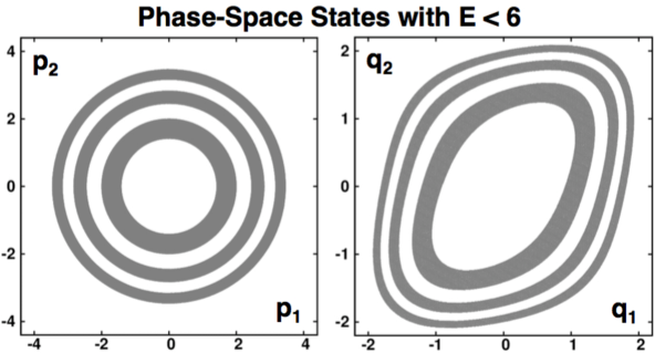
Figure 1: When the two-body $\phi^{4}$ model has an energy of 6, the momenta are confined to the region $p_{1}^{2}+p_{2}^{2}<12$ shown at the left. The displacement coordinates of the particles, $q_{1}$ and $q_{2}$, are confined to the region shown to the right. The contours shown here correspond to the energies 1 through 6. $E=[\ p_{1}^{2}+p_{2}^{2}+q_{1}^{2}+(q_{1}-q_{2})^{2}\ ]/2+(\ q_{1}^{4}+q_{2}^{4}\ )/4<6\ .$ Most of the three-dimensional microcanonical energy shell between $E=6$ and $E=6+dE$ corresponds to stable tori.

I The Simplest $\phi^{4}$ Chain and the 2018 SNOOK Prizes

The 2017 Snook Prize has already shed considerable light on small-system implementations of Kenichiro Aoki and Dimitri Kusnezov’s $\phi^{4}$ Modelb1 . Besides providing transparent time-reversible examples of nonequilibrium heat flows the model illustrates several varieties of broken symmetries in both space and time, as discussed elsewhere in this issue of Computational Methods in Science and Technology.b2 ; b3 Figure 1 shows equally-spaced contours of the kinetic and potential energies of the model.

For simplicity, in this work we take initial conditions where the energy is entirely kinetic, $q_{1}=q_{2}=0\ ;\ p_{1}^{2}+p_{2}^{2}=12$. The examples here correspond to the same energy states studied by Aoki and illustrated in Figures 6 and 7 of his prize-winning contribution for last year’s Snook Prizesb2 ; b3 .

In that same competition Timo Hofmann and Jochen Merker discovered two coexisting chaotic seas in a fourteen-term polynomial generalization of the Hénon-Heiles model’s cubic Hamiltonianb4 . In our follow-up exploration of the two-body $\phi^{4}$ model we have found two coexisting chaotic seas. Specimens of both are shown in Figures 2 and 3. Evidently the present simplest of chaotic Hamiltonians, with only seven polynomial energy contributions, is enough to support the coexistence of the seas.

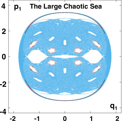
Figure 2: A projected section of the “Large” sea generated with initial conditions $(q_{1},q_{2})=(0,0)$ and $(p_{1},p_{2})=(\sqrt{12},0)$ is shown in blue. Most of the phase space at this energy corresponds to tori. The two examples shown here correspond to initial momenta of $(\sqrt{(11.9,0.1)}$ and $(\sqrt{(11.8,0.2)}$, with each point on the closed curves plotted when the trajectory passes through the $q_{2}=0$ hyperplane.

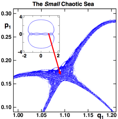
Figure 3: Here the initial condition is $(q_{1},q_{2})=(0,0)$ and $(p_{1},p_{2})=(\sqrt{(11.4,0.6)}$ and the projection onto the $(q_{1},p_{1})$ plane is done whenever $q_{2}=0$. The full projection is shown in the upper left inset, where $|\ q_{1}\ |<2$. An enlargement shows that the apparent crossing lines in the inset actually correspond to “fat fractal” regions with a nonvanishing Lyapunov exponent, $\lambda_{1}=0.003_{0}$, where the simulation was extended for $10^{11}$ timesteps in order to get a reliable value of the exponent.

II Chaos in the Two-Mass $\phi^{4}$ Chains

Relatively long calculations with $10^{11}$ timesteps showed that both of the problems solved in Figures 2 and 3 are chaotic. We used the same reference trajectory + rescaled-satellite trajectory algorithm discovered independently by groups in Italy and Japanb5 ; b6 . The small sea in Figure 3 corresponds to a Lyapunov exponent of 0.003. The large sea of Figure 2 is much less stable, with a time-averaged exponent $\lambda_{1}=0.05$. We wish to emphasize that these two values correspond to exactly the same energy, 6, and only differ in the initial values of $p_{1}$ and $p_{2}$. The Lyapunov-exponent description of the divergence of two nearby trajectories is defined by the rate equations $\{\ \dot{\delta}=\lambda_{1}\delta\ \}$, where the separation $\delta$ is measured in phase space :

$$\delta\equiv\sqrt{\delta_{q_{1}}^{2}+\delta_{q_{2}}^{2}+\delta_{p_{1}}^{2}+\delta_{p_{2}}^{2}}\ .$$

The rescaling algorithm brings the satellite trajectory to the same distance, $\delta\rightarrow 0.00001$, after each timestep. We use fourth-order or fifth-order Runge-Kutta integrators with $dt=0.001$ throughout.

Figure 4 shows the momenta for a time interval $0<{\rm time}<20$ for the large and small seas. It is a little paradoxical that the less stable large-sea trajectory (at the left, with $\lambda_{1}=0.05$) apparently explores less of the $(p_{1},p_{2})$ region than does the more-stable $\lambda_{1}=0.003_{0}$ small-sea trajectory.

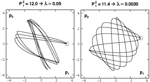
Figure 4: Starting with two circled initial conditions $(p_{1}^{2}=12\ ;\ p_{2}^{2}=0)$ and $(p_{1}^{2}=11.4\ ;\ p_{2}^{2}=0.6)$ we show the $(p_{1},p_{2})$ trajectory projections in momentum space up to a time of 20. These two trajectories are both chaotic, but with very different Lyapunov exponents.

The three-dimensional energy surface in four-dimensional phase space, $\{\ q_{1},p_{1},q_{2},p_{2}\ \}$ is difficult to visualize. Lacking a clever coordinate transformation we can only project or cut. Investigation of two-dimensional projections on the six two-dimensional planes provided by the four state variables shows that much of the surface is composed of tori. For initial conditions with all or nearly all of the kinetic energy given to Particle 1 at least two chaotic seas occur. The sections in Figure 5 show the chains of islands typical of Hamiltonian chaos as well as the structures corresponding to simple elliptic doughnuts. It appears that the chaotic regions correspond to three-dimensional “fat fractals”b7 . The sections provide plenty of room for further exploration.

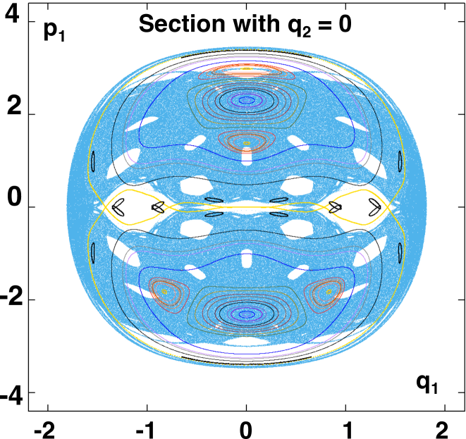
Figure 5: Here we see penetrations of the $(q_{1},p_{1})$ plane along trajectories of 50,000,000 timesteps each using 25 equally-spaced initial conditions, $p_{1}^{2}=0,\ 0.5,\ 1.0,\ 1.5,\ \dots 12$ and $p_{1}^{2}+p_{2}^{2}=12$. This $q_{2}=0$ projection shows traces of many tori as well as a black “chain of islands”. The last of these initial conditions produces the blue dots, which form the largest fat-fractal chaotic sea. Most of the remaining points are closed curves generated by stable tori. Note the 18 black curves mostly near $p_{1}=0$ which correspond to a relatively complex torus which threads through the $q_{2}=0$ hyperplane eighteen times. The corresponding initial momenta are $p_{1}^{2}=11.5\ ;\ p_{2}^{2}=0.5$ .

III Thermodynamics and the Ideal-Gas Thermometer

It is interesting to see that the time-averaged kinetic temperatures of the two particles, $T_{i}=\langle\ p_{i}^{2}\ \rangle$, are quite different in both the large unstable and the small more stable chaotic seas. A permanent temperature difference in a stationary equilibrium system suggests thought-experiments violating the Second Law of Thermodynamics. Evidently ideal-gas thermometers, though validated by kinetic theoryb8 cannot be entirely consistent with equilibrium thermodynamics. This subject is complicated by the fact that nonequilibrium fractal distributions (typically found for time-reversible steady states)b9 correspond to a divergence of the Gibbs entropy $S$, making the usual equilibrium definition of temperature, $(\partial E/\partial S)_{V}$, useless.

It is important to see that for any choice of the pair of coordinates $\{\ q_{1},q_{2}\ \}$ Gibbs’ statistical mechanics establishes that the maximum-entropy distributions of the two momenta $\{\ p_{1},p_{2}\ \}$ are identical. Thus our finding $\langle\ T_{1}\ \rangle\neq\langle\ T_{2}\ \rangle$ shows that the dynamics from Hamilton’s motion equations is not at all ergodic. For example, in the large chaotic sea the mean values of the kinetic temperatures of the two particles are roughly $(3.7_{4},3.1_{7})$. Whether or not there is a simple and useful deterministic time-reversible ergodic algorithm for the microcanonical distribution is (we think) unknown. Perhaps an analog of magnetic-field rotational forces would be useful in developing such an algorithm ?

IV The Snook Prize Problem for 2018

The several previous $\phi^{4}$ studies, carried out with a variety of system sizes and thermostatted boundary conditionsb10 , have established that the $\phi^{4}$ model can be usefully described by Fourier’s Law. These works also demonstrate that nonequilibrium phase-space distributions are fractal attractors, with dimensionalities which can lie far below the dimensionality of Gibbs’ equilibrium distributionsb9 . A systematic study could be made to show how the distribution of temperatures in a conducting chain approaches the Law as the number of degrees of freedom is increased beyond two. The two-body problem itself suggests a study of the phase-space boundaries separating the regions of chaos from regular tori and an analysis of the disappearance of the tori with increasing energy. The possibility of developing a time-reversible ergodic algorithm at constant energy has to be considered. A study of clever ideas for the model would be welcome. The Snook Prize Problem is a detailed investigation of the two-body $\phi^{4}$ problem from the standpoints of Hamitonian chaos and Kolmogorov-Arnold-Moser tori and from the goal of an isoenergetic algorithm for the microcanonical Gibbs ensemble. It is particularly desirable that Prize entries be self-contained and pedagogical, stressing numerical findings in sufficient detail that their results can be corroborated.

V Acknowledgments

We are grateful to the Institute of Bioorganic Chemistry of the Polish Academy of Sciences and to the Poznan Supercomputing and Networking Center for their joint support of these prizes honoring our late Australian colleague Ian Snook (1945-2013).

References

- (1) K. Aoki and D. Kusnezov, “Lyapunov Exponents and the Extensivity of Dimensional Loss for Systems in Thermal Gradients”, Physical Review E 68, 056204 (2003).
- (2) K. Aoki, “Symmetry, Chaos, and Temperature in the One-Dimensional Lattice Theory”, Computational Methods in Science and Technology 24 (2018) = ariv 1801.02865. His ariv version 1 contains the configurational part of our Figure 1. That figure is missing in version 2 and the internet version in CMST.
- (3) Wm. G. Hoover and C. G. Hoover, “The 2017 SNOOK PRIZES in Computational Statistical Mechanics”, Computational Methods in Science and Technology 24 (2018).
- (4) T. Hofmann and J. Merker, “On Local Lyapunov Exponents of Chaotic Hamiltonian Systems”, Computational Methods in Science and Technology 24 (2018).
- (5) G. Benettin, L. Galgani, A. Giorgilli, and J.-M. Strelcyn, “Lyapunov Characteristic Exponents for Smooth Dynamics Systems and for Hamiltonian Systems; a Method for Computing All of Them, Parts I and II: Theory and Numerical Application”, Meccanica 15, 9-20 and 21-30 (1980).
- (6) I. Shimada and T. Nagashima, “A Numerical Approach to Ergodic Problems of Dissipative Dynamical Systems”, Progress of Theoretical Physics 61, 1605-1616 (1979).
- (7) J. D. Farmer, E. Ott, and J. A. Yorke, “The Dimension of Chaotic Attractors”, Physica D 7, 153-180 (1983).
- (8) Wm. G. Hoover and C. G. Hoover, “Nonequilibrium Temperature and Thermometry in Heat-Conducting Models”, Physical Review E 77, 041104 (2008).
- (9) Wm. G. Hoover and C. G. Hoover, Microscopic and Macroscopic Simulation Techniques – Kharagpur Lectures, Section 10.8 (World Scientific Publishers, Singapore, 2018).
- (10) Wm. G. Hoover, K. Aoki, C. G. Hoover, and S. V. De Groot, “Time-Reversible Deterministic Thermostats”, Physica D 187, 253-267 (2004).