Pre-seismic ionospheric anomalies detected before the 2016 Taiwan earthquake

Abstract

On Feb. 5 2016 (UTC), an earthquake with moment magnitude 6.4 occurred in southern Taiwan, known as the 2016 (Southern) Taiwan earthquake. In this study, evidences of seismic earthquake precursors for this earthquake event are investigated. Results show that ionospheric anomalies in Total Electric Content (TEC) can be observed before the earthquake. These anomalies were obtained by processing TEC data, where such TEC data are calculated from phase delays of signals observed at densely arranged ground-based stations in Taiwan for Global Navigation Satellite Systems. This shows that such anomalies were detected within 1 hour before the event.

1 Introduction

The ionosphere is an ionized medium which can affect the radio communications. The electron density in the ionosphere is disturbed by various phenomena such as solar flares [Donnelly(1976)], volcanic eruptions [Igarashi et al.(1994)], flying objects [Mendillo et al.(1975)], earthquakes [Ogawa et al.(2012)], and so on. These electron density disturbances are observed with Total Electron Contents (TECs) at ground-based Global Navigation Satellite Systems (GNSS) receivers. With GNSS that can monitor variations of TEC, it has been reported [Heki(2011), Heki and Enomoto(2015)] that pre-seismic ionospheric electron density anomalies appeared frequently before large earthquakes, which could be caused by the earthquake-induced electromagnetic process before such earthquakes. Furthermore, such TEC anomalies were found in the 2016 Kuramoto earthquake (Mw7.3) [Iwata and Umeno(2017)].

Taiwan is located in an active seismic area [Liu et al(2000), Oyama et al.(2008)] and has ground-based stations for GNSS with densely arranged receivers. Thus, Taiwan is a suitable region to explore relations between earthquakes and pre-seismic ionospheric TEC anomalies. Also, Taiwan has been focused from a viewpoint of electric currents in the earth crust and electromagnetic emissions preceding to earthquakes [Freund(2003)]. An earthquake occurred around southern Taiwan in Feb. 2016 (19:57 UT, 5 Feb. 2016, Mw6.4, depth $23.0$ km, $22.94$ N $120.6$ E ). As reported in U.S. Geological Survey [USGS(2016)], this event was the result of oblique thrust faulting at shallow-mid crustal depths. Rupture occurred on a fault oriented either northwest-southwest, and dipping shallowly to the northeast, or on a north-south striking structure dipping steeply to the west. At the location of the earthquake, 2 tectonic plates converge in a northwest-southeast direction at a velocity of about $80$ mm a year.

In this paper pre-seismic ionospheric TEC anomalies for the 2016 Taiwan earthquake (Mw6.4) are shown with the method described in [Iwata and Umeno(2016)]. This analysis is referred to as CoRelation Analysis (CRA) in this paper. With CRA, the TEC anomalies were detected for the Kuramoto earthquake [Iwata and Umeno(2017)], where this earthquake is classified as an intraplate earthquake and its moment magnitude is less than Mw 8.0. It is then of interest to explore if TEC anomaly is observed with this method for intraplate earthquakes whose moment magnitudes are less than Mw 7.0. After TEC anomalies will be shown in this paper, a possible link connecting satellite tracks with an assumed ionospheric anomaly area over Taiwan will be argued. This is to investigate why such anomalies can be observed with some specific satellite tracks ( See Figure 1).

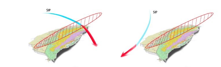
Figure 1: (left) When a Sub-Ionospheric Point (SIP) track crosses the projection of an assumed ionospheric anomaly area (shaded in red). (right) When a SIP track does not cross the projection of the anomaly area.

2 Method

The TEC along the line of sight, called slant TEC, can be calculated with the phase delay of signals sent from GNSS satellites observed at ground-based GNSS receivers. In the following slant TEC is abbreviated as TEC, and TEC data are calculated from signals sent from the Global Positioning System (GPS, American GNSS) satellites. Also, the standard unit for TEC, TECU that is $10^{16}$ el/$m^{2}$, is used. For simplifying various calculations, electrons in the ionosphere are approximated to be in a thin layer, and this layer for Taiwanese GNSS stations is set to $325$ km above the ground. At this altitude, the electron density is the maximum in the ionosphere. The intersection of the line of sight from a GNSS receiver with this thin layer is called Ionospheric Piercing Point (IPP), and its projection onto the surface of the earth is called Sub-Ionospheric Point (SIP). SIP tracks for Taiwanese GNSS stations shown in this paper were calculated with this altitude of the thin layer.

For large earthquakes the CoRrelation Analysis (CRA) was shown to detect earthquake precursors [Iwata and Umeno(2016)]. The analysis, CRA, is based on calculating correlations among TEC values, where how to calculate these correlations is summarized as follows.

1. Choose a central GNSS station, a satellite, and 3 parameters denoted by $t_{\,\mathrm{sample}}$, $t_{\,\mathrm{test}}$, and $M$. The parameter $t_{\,\mathrm{sample}}$ is the time-length of data used for obtaining a regression curve, $t_{\,\mathrm{test}}$ the time-length for testing the difference between the regression curve and the obtained data, and $M$ the number of GNSS stations located around the central station for the correlation analysis. We fix $t_{\,\mathrm{sample}}$ and $t_{\,\mathrm{test}}$ to be $2$ and $0.25$ h throughout this paper.

2. Let SampleData be the TEC data for the time-duration from $t$ to $t+t_{\,\mathrm{sample}}$ for each station labeled by $i$. Also, let TestData be the TEC data for the time-duration from $t+t_{\,\mathrm{sample}}$ to $t+t_{\,\mathrm{sample}}+t_{\,\mathrm{test}}$.

3. Fit a curve to SampleData by the least square method with a polynomial curve whose degrees is 7.

4. Calculate a deviation of TestData from the regression curve for the time-duration $t_{\,\mathrm{test}}$, and such a deviation is denoted by $x_{i,t^{\prime}}$ where $t^{\prime}$ is such that $t_{\,\mathrm{sample}}\leq t^{\prime}\leq t_{\,\mathrm{sample}}+t_{\,\mathrm{test}}$.

5. Calculate the correlation defined as

   $$C(T)=\frac{1}{NM}\sum_{i=1}^{M}\sum_{j=0}^{N-1}x_{\,i,t+t_{\mathrm{sample}}+j\Delta t}\,x_{\,0,t+t_{\mathrm{sample}}+j\Delta t},$$

   where $T=t+t_{\,\mathrm{sample}}+t_{\,\mathrm{test}}$, $N$ is the number of data points for TestData, $\Delta\,t=30$ sec the sampling interval for TestData so that $\Delta\,t=t_{\,\mathrm{test}}/(N-1)$, and $i=0$ the special label indicating the central GNSS station. The physical dimension of $C(T)$ is the square of TECU.

In what follows the word “anomaly” is used, when the correlation value is high enough. To quantify and define abnormality, careful discussions are needed. Thus, we compare correlation values in view of days, SIP tracks, and distances among GNSS stations. The details of these are discussed in Section 3.

3 Data Presentation

In this section (i) raw TEC data and (ii) correlations are shown with respect to GNSS ground-based stations, and with respect to GPS satellites 17 and 28. A variety of choices for stations and satellites enables one to argue how TEC anomalies can be observed with respect to the SIP track. For this reason GNSS stations were chosen from the south, middle, and north of Taiwan.

TEC data were obtained from the original GPS data with the method in [Otsuka et al.(2002)], and the original GPS data were obtained from the Central Weather Bureau (CWB) in Taiwan.

3.1 Results for the event day

In this subsection results for the event day are shown. The parameter $M$ was chosen to be $1$, which is equivalent to $2$ GNSS stations for CRA.

3.1.1 Stations in the south of Taiwan

Figure 2 shows results for stations located in the south of Taiwan. We chose “gais” as the central station, since it is the nearest station from the epicenter. The distance is about $1.0$ km. The other station for CRA is “wanc”, and it is the next nearest station for which TEC data were available. The distance between “wanc” and the epicenter is about $14.1$ km. From the left panels, the SIP tracks for GPS satellite 17 crossed the projection of the assumed ionospheric anomaly area, and most of the SIP tracks for GPS satellite 28 did not cross it. ( See figure 1 ). From the middle panels, it is verified that the obtained $2$ time-series of TEC data were similar to each other. It is reasonable, since these 2 stations are geographically close. Time-series of correlations were obtained by processing this kind of TEC data. As it can be read off from the right upper panel showing correlations obtained with CRA for GPS satellite 17, about 40 min before the event, a period of time was observed where correlation values are high. Its maximum value was $123$, which was observed at 19:23 UT. Besides, as can be seen from the right panels, the correlation values for GPS satellite 28 were lower than those of 17. This comparison between the time-series of correlations indicates that how TEC anomalies can be observed is with respect to the SIP track ( See Section 4 for discussions ).

In the following, to explore a spatial dependency of TEC anomalies, we show TEC data and their correlations with CRA obtained at stations located other areas in Taiwan.

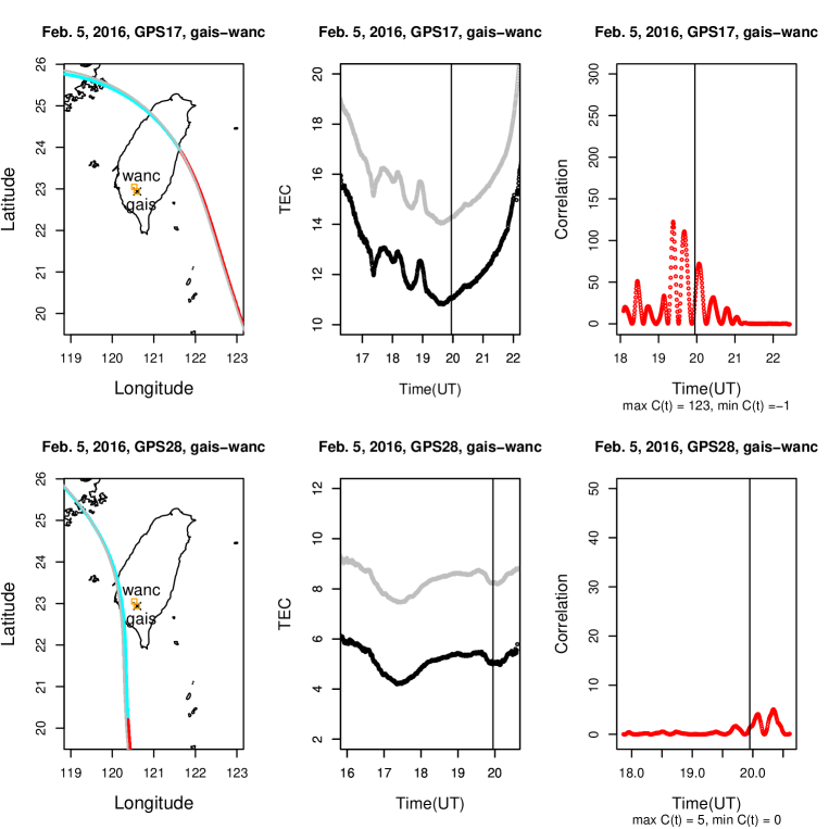
Figure 2: (left) SIP tracks for GPS satellites 17 and 28. Red: Track for “gais” after the event, Cyan: Track for “gais” before the event, Gray: Track for “wanc”, $\times$: Epicenter. (middle) Time series of TEC, the vertical lines indicate the time (UT) when the event occurred. Black: TEC obtained at “gais”, Gray: TEC obtained at “wanc”, where the TEC values were shifted by hand for the guide of eyes. (right) Time series of correlations obtained with CRA.

3.1.2 Stations in the middle of Taiwan

Figure 3 shows results for stations located in the middle of Taiwan. We chose “huys” as the central station for CRA, and the other station was “guk2”. The distance between these stations is about $12.4$ km, and that between the epicenter and “huys” is about $120.2$ km. From the left panels, SIP tracks for GPS satellite 28 crossed the projection of the anomaly area, which was contrary to the case of the south of Taiwan. The SIP tracks for GPS satellite 28 was north-south, which was different from the case for 17. It can be seen from the right panels, as well as the case of the south stations, correlation values associated with GPS satellite 17 were higher than those with 28. The maximum correlation value associated with the satellite 17 was 176, which was observed at 19:26 UT. Notice that the correlation values associated with GPS satellites 17 and 28 became higher than those for the south stations.

In the following, to see more details of this spatial dependency, we focus on TEC data and their correlations obtained with CRA for stations located in the north of Taiwan.

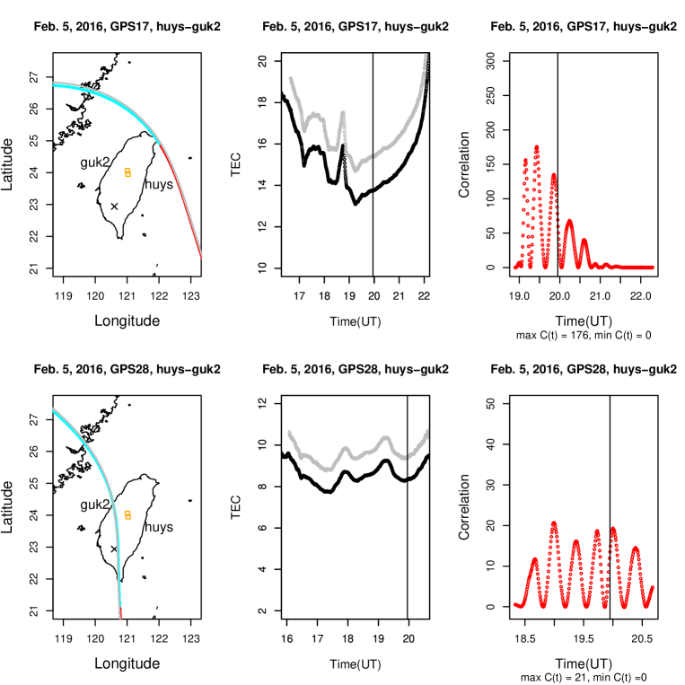
Figure 3: (left) SIP tracks for GPS satellites 17 and 28. Red: Track for “huys” after the event, Cyan: Track for “huys” before the event, Gray: Track for “guk2”, $\times$: Epicenter. (middle) Time series of TEC, Black: TEC obtained at “huys”, Gray: TEC obtained at “guk2”, where the TEC values were shifted by hand for the guide of eyes. (right) Time series of correlations obtained with CRA.

3.1.3 Stations in the north of Taiwan

Figure 4 shows results for stations located in the north of Taiwan. We chose “ankn” as the central station for CRA, and the other station was “lnko”. The distance between these stations is about $19.4$ km, and that between the epicenter and “ankn” is about $227.3$ km. From the left panels, the SIP tracks for GPS satellites 17 and 28 crossed the projection of the assumed anomaly area. The maximum correlation value associated with the satellite 17 was 301, which was observed at 19:14 UT. Notice from the right panels that the correlation values associated with GPS satellites 17 and 28 were higher than those for the stations located in the south and middle.

In the next subsection the details of TEC anomalies are argued. In particular, how correlations depend on $M$, whether or not TEC anomalies were observed before the event day, and so on, are focused.

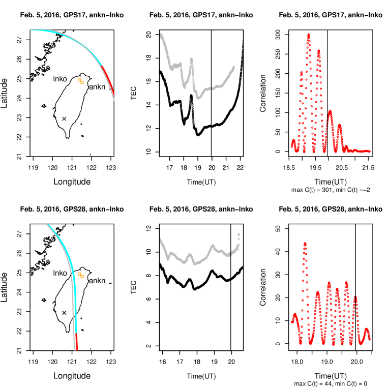
Figure 4: (left) SIP tracks for GPS satellites 17 and 28. Red: Track for “ankn” after the event, Cyan: Track for “ankn” before the event, Gray: Track for “lnko”, $\times$: Epicenter. (middle) Time series of TEC, Black: TEC obtained at “ankn”, Gray: TEC obtained at “lnko”, where the TEC values were shifted by hand for the guide of eyes. (right) Time series of correlations obtained with CRA.

3.2 Detailed results for the south stations

In the previous subsection, TEC anomalies were found about 40 min before the event on Feb. 5, where $M=1$ was used for CRA. To see if such anomalies occurred days before the event or not, we show TEC data and their correlations with particular focus on the south stations. For the same purpose, $M$ dependency of correlations are shown as well.

3.2.1 TEC data for days before the event

Figure 5 shows the time-series of TEC data observed for the consecutive 9 days including the event day. These time-series were obtained with GPS satellite 17 associated with the stations “gais” and “wanc”. From this figure, it is verified that the obtained $2$ time-series on each day were similar.

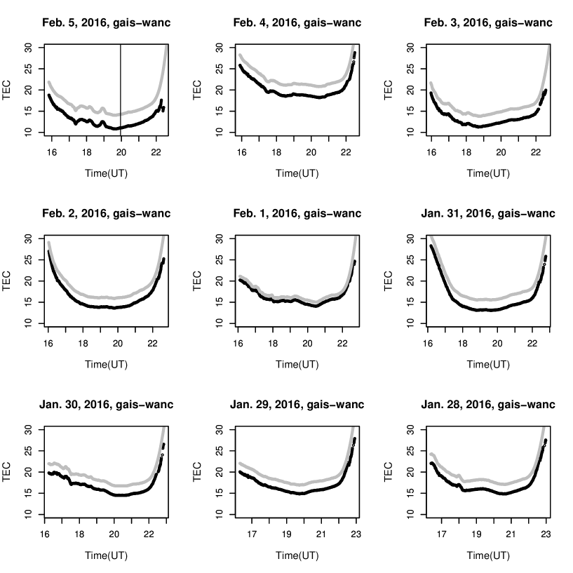
Figure 5: Time-series of TEC data observed at the stations “gais” (black) and “wanc” (gray) for the period from Jan. 28 to Feb. 5 in 2016, where the TEC values obtained at “wanc” were shifted by hand for the guide of eyes. GPS satellite 17 was used, and the vertical line on Feb. 5 indicates the time when the event occurred.

Figure 6 shows the time-series of TEC data observed for the consecutive 9 days including the event day. These time-series were obtained with GPS satellite 28 associated with the stations “gais” and “wanc”. As well as the case of GPS satellite 17 ( See Figure 5), it is verified that the obtained $2$ time-series on each day were similar. On the event day, time-series of TEC data were smoother than those of GPS satellite 17. This smoothness yields low correlation values obtained with CRA. On Feb. 1, the time-series of TEC data were not smooth to some extent, and they were consistent with the case of GPS satellite 17.

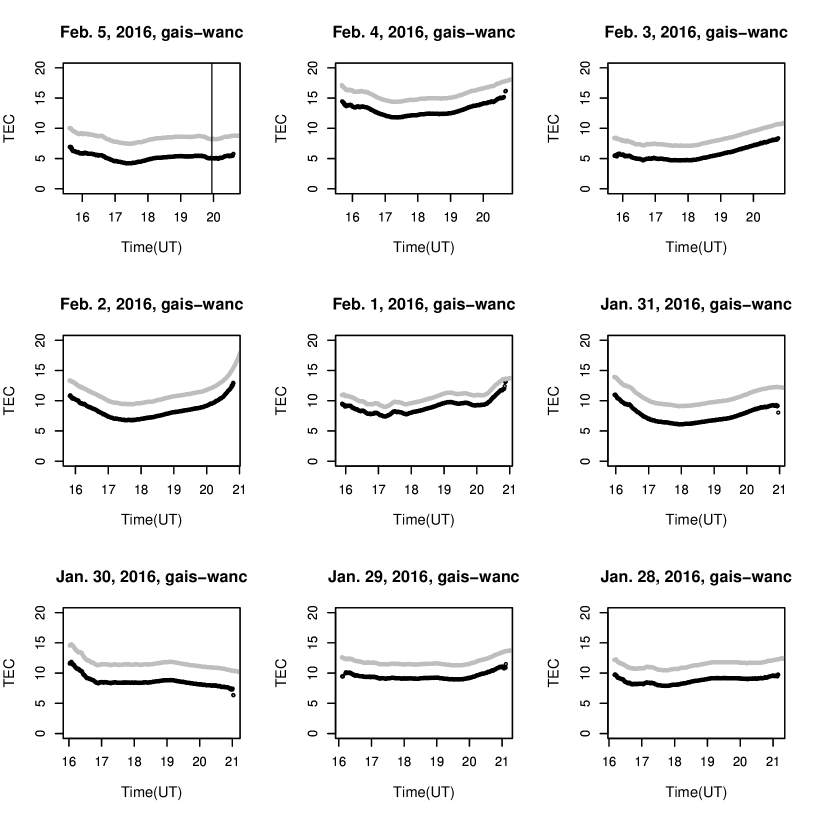
Figure 6: Time-series of TEC data observed at the stations “gais” (black) and “wanc” (gray) for the period from Jan. 28 to Feb. 5 in 2016, where the TEC values obtained at “wanc” were shifted by hand for the guide of eyes. GPS satellite 28 was used, and the vertical line on Feb. 5 indicates the time (UT) when the event occurred.

3.2.2 Correlations with $M=1$ and GPS 17 and 28 (From Jan. 28 to Feb. 5)

Figure 7 shows the time-series of correlations obtained by CRA with $M=1$ and GPS satellite 17 for the consecutive $9$ days including the event day. There were some periods where correlation values are high on Jan. 28 and Feb. 1. On Jan. 28, this anomalous period was situated around the time when time-series started. In addition the maximum value of the correlation on Jan. 28 was about half of that on Feb. 5. On Feb. 1, the maximum value of the correlation obtained by CRA was $1/3$ of that on Feb. 5. All the time-series of correlations obtained by CRA in this figure are compared with those for the case of $M=5$ in figure 9.

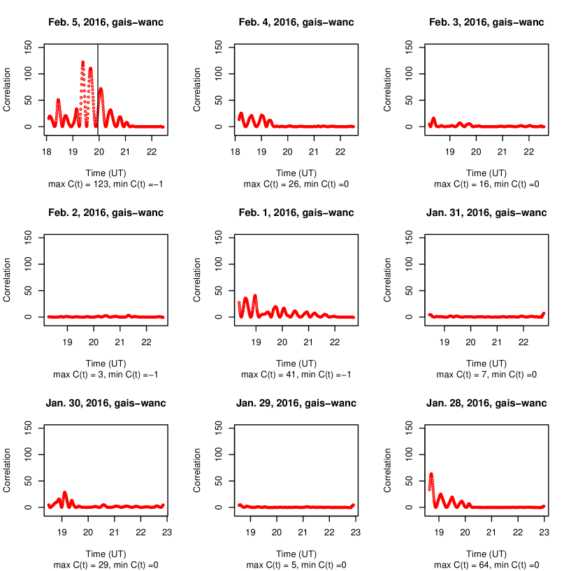
Figure 7: Time-series of correlations obtained by CRA with $M=1$, where TEC data were observed at the stations “gais” and “wanc” for the period from Jan. 28 to Feb. 5 in 2016. GPS satellite 17 was used. The vertical line on Feb. 5 indicates the time when the event occurred.

Figure 8 shows the time-series of correlations obtained by CRA with $M=1$ and GPS satellite 28 for the consecutive $9$ days including the event day. There were some periods where correlation values are high on Feb. 1. Note that this period also occurred on this day for the case of GPS satellite 17. Although no figure is given, it can be shown that correlation values with GPS satellite 28 on Feb. 1 did not decrease for the case with $M=5$.

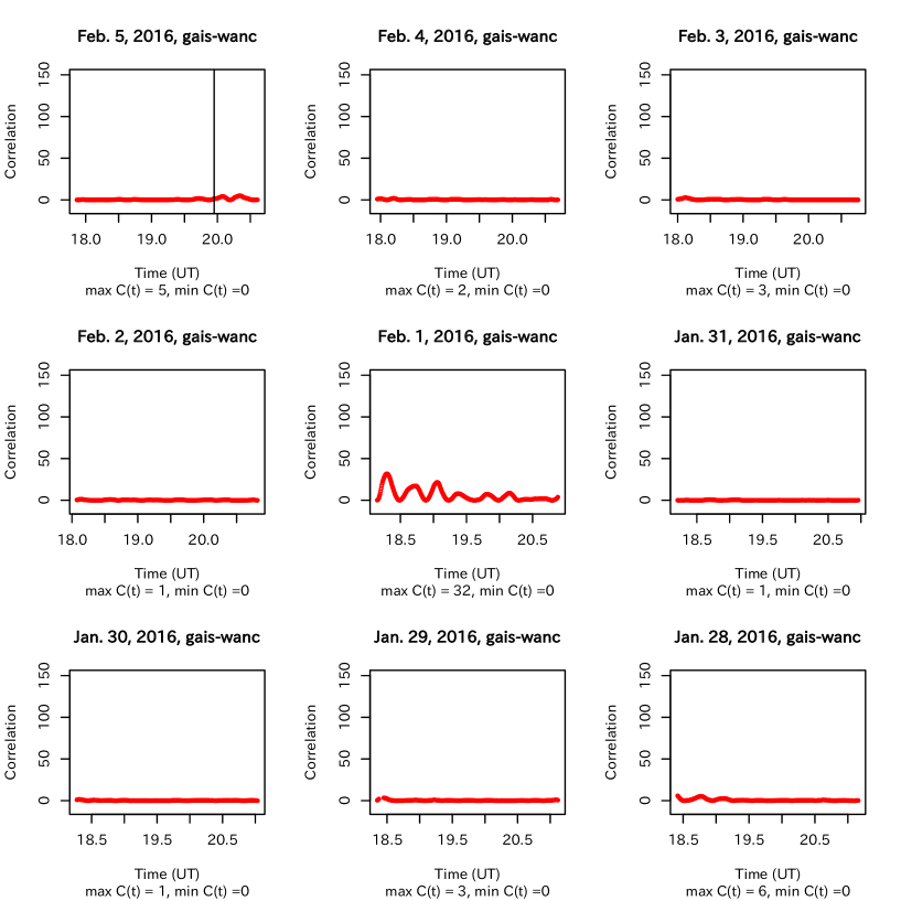
Figure 8: Time-series of correlations obtained by CRA with $M=1$, where TEC data were observed at the stations “gais” and “wanc” for the period from Jan. 28 to Feb. 5 in 2016. GPS satellite 28 was used. The vertical line on Feb. 5 indicates the time when the event occurred.

3.2.3 Correlations with $M=5$ and GPS17 (From Jan. 6 to Feb. 5)

Figure 9 shows the time-series of correlations obtained by CRA with $M=5$ for the consecutive 9 days including the event day. The central station is “gais” that is the nearest one from the epicenter. The other stations were chosen as “wanc”, “jwen”, “mlo1”, “dani”, and “shwa” so that they are located near the epicenter. When the number of stations for the correlation analysis increases, it is expected that the correlation values become higher than those with $M=1$, if each station receives common sudden disturbed signals. On the event day, the obtained time-series is consistent with the case with $M=1$ in Figure 7. For the days Feb. 1 and Jan. 28, on which correlation values were high but no event, the maximum values decreased by more than half of those with $M=1$. Combining these, we see that the anomaly in time-series on Feb. 5 appeared commonly around the central station “gais”. On the contrary, anomalies on Feb. 1 and Jan. 28 did not appear commonly around “gais” for the SIP track for GPS satellite 17.

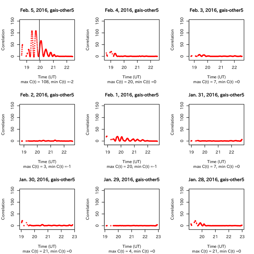
Figure 9: Time-series of correlations obtained by CRA with $M=5$, where TEC data were observed at 6 stations for the period from Jan. 28 to Feb. 5 in 2016. GPS satellite 17 was used, and the central station is “gais”, and the other 5 stations are “wanc”, “jwen”, “mlo1”, “dani”, “shwa”. The vertical line on Feb. 5 indicates the time (UT) when the event occurred.

Figure 10 shows time-series of correlations obtained by CRA with $M=5$ for the period from Jan. 17 to Jan. 27 in 2016, except for Jan. 24 and 25. On Jan. 24 and 25, no data were acquired. No significant anomaly was observed in this period, and this observation is consistent with the non-existence of significant geomagnetic activity ( see Section 4 ).

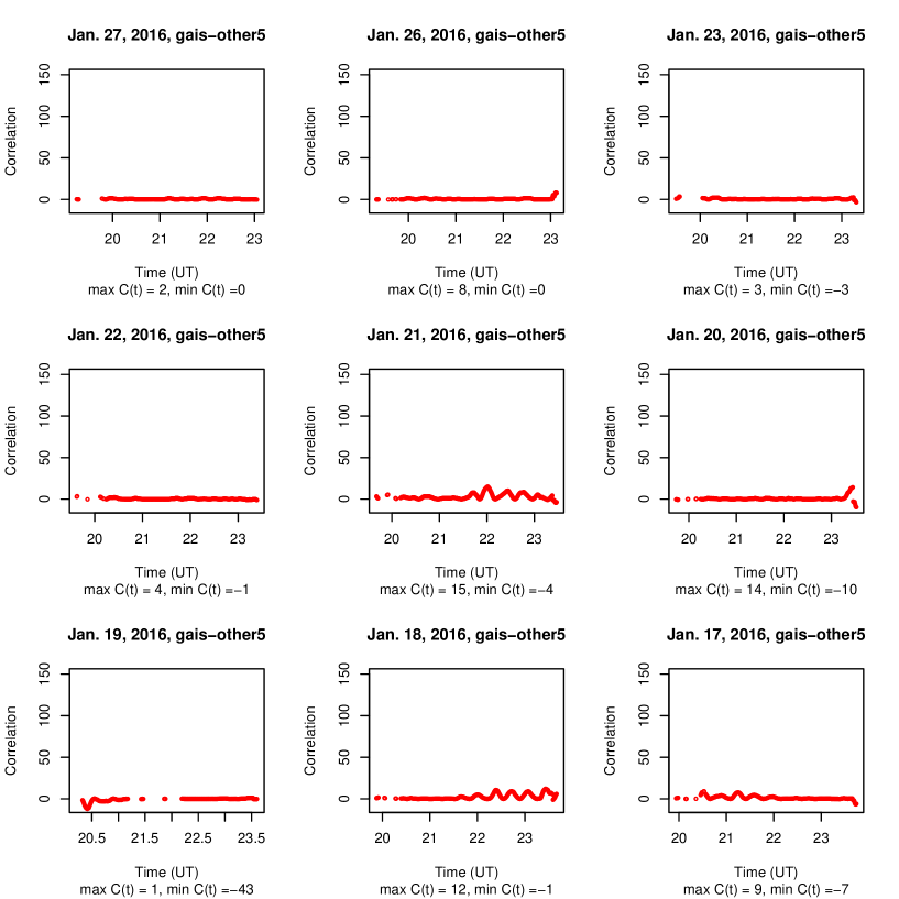
Figure 10: Time-series of correlations obtained by CRA with $M=5$ for the period from Jan. 17 to Jan. 27 in 2016, except for Jan. 24 and 25, at the stations described in the caption of Figure 9. GPS satellite 17 was used.

Figure  11 shows time-series of correlations obtained by CRA with $M=5$ for the period from Jan. 6 to Jan. 16 in 2016, except for Jan. 7 and 8. On Jan. 7 and 8, no data were acquired. On Jan. 12th, there were some periods where correlation values are higher than those on the other days in this figure. Although no figure is given, it can be shown that such correlation values were lower than those with $M=1$ for GPS satellite 17. This reduction of correlation values as $M$ increases is consistent with the case where there was no significant seismic activity around the island.

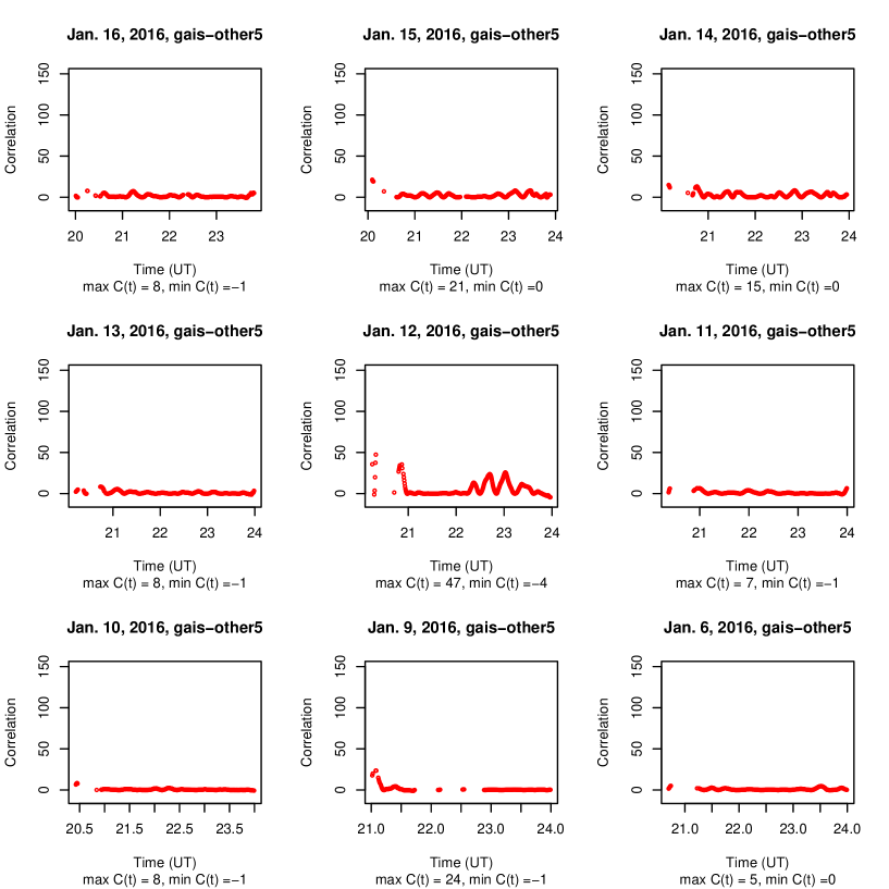
Figure 11: Time-series of correlations obtained by CRA with $M=5$, where TEC data observed at the stations described in the caption of figure 9 for the period from Jan. 6 to Jan. 16 in 2016, except for Jan. 7 and 8. GPS satellite 17 was used.

4 Discussion

TEC anomalies before the earthquake have been shown in Section 3. To give another evidence that such TEC anomalies were caused by the Taiwan earthquake, our correlation analysis can also be applied to time-series of TEC data obtained in Japan on the event day. GNSS data were obtained from the Geospatial Information Authority of Japan. The distance between Taipei and Fukuoka located the south part of Japan is about $1280$ km, and the correlation analysis applied to TEC data observed in Japan provides how much Medium-Scale Traveling Ionospheric Disturbance (MSTID) occurred, where Japan is located upstream of MSTID[Hunsucker(1982), Otsuka et al.(2011)]. Here MSTID is known as a type of disturbance in the ionosphere, and it might hide TEC anomalies as an earthquake precursor.

Figure 12(a) shows the time-series of correlations with $M=30$ obtained with TEC data observed at various GNSS stations in Japan 30 min before the event, where TEC data were obtained with GPS satellite 28. It suggests that there was no significant TEC anomaly and MSTID around Japan. Figure 12(b) shows the SIP track from GPS satellite 28 for the GNSS station “0087”, Fukuoka in Japan. The altitude for calculating SIP is $300$ km above the ground. From these data concerning the upstream of MSTID, there was no disturbance due to MSTID around the time when the anomalies in Taiwan were observed.

Geomagnetic variations indices of Kp and Dst are examined during a month, from Jan. 5 to Feb. 5 2016, on this earthquake day and earlier. Provisional Dst indices show variations between $-53$ and $17$ from Jan. 23 to Feb. 5, and those between $-93$ and $19$ from Jan. 5 to Jan. 22. No Sudden Storm Commencement was observed from Jan. 23 to Feb. 5, and then this period was under relatively quiet geomagnetic conditions. Therefore it is presumed that the analyzed period of TEC variations were not contaminated by relatively large geomagnetic disturbances. On the other hand, although some geomagnetic disturbance occurred from Jan. 5 to Jan. 22, it did not affect the correlation values obtained by CRA, since the maximum Kp index was observed around Jan. 21, and there was no high correlation value around Jan. 21 ( See Figure 10 ).

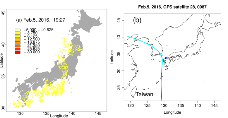
Figure 12: (a) Time-seriese of correlations obtained by CRA with $M=30$, where TEC data were observed at various stations in Japan at 19:27 UT on Feb. 5, 2016. Here GPS satellite 28 was used. (b) SIP track from GPS satellite 28 for “0087” (“Koga” in Fukuoka, blue, $\blacksquare$ ). Cyan curve: SIP track before the event, and Red curve: SIP track after the event.

To explain TEC anomalies responsible for large earthquakes, several models consisting of electromagnetic processes due to stressed rocks have been proposed. Recent progress of such has been summarized in [He and Heki(2017)]. Such models are Lithosphere-atmosphere-ionosphere (LAI) coupling models, and one of them is based on the experimental results on stressed rocks [Freund(2013)]. In [Heki and Enomoto(2015)], differences between intraplate earthquakes and interplate ones with Mw$\geq 8.2$ were argued, and then each mechanism that causes precursors could be different each other. Since the focus of this study is an intraplate earthquake with Mw6.4, the existing models proposed so far for observed TEC anomalies may not be suitable.

As shown in the previous section, SIP tracks could be related to how TEC anomalies are observed. To explore such a relation, assume that some enough amount of electric currents in the earth crust exist before relatively large earthquakes [Freund(2003)]. From this, electromagnetic fields are induced in the ionosphere. If an IPP track crosses an assumed ionospheric anomaly area, then TEC is disturbed by the induced electromagnetic field ( See Figure 1 ). This disturbance causes the emergence of high correlation values, which is consistent with our results. For quantitative discussions, a physical model is needed for future study.

This assumption of electromagnetic fields can deny a possibility that solar activity contributed to TEC anomalies on the event day. This is argued by showing a contradiction from an assumption. Assume first that an intensive solar activity contributes to TEC anomalies. Then correlation values obtained by CRA with respect to each satellite should equally be affected, i.e., how TEC anomalies are observed should not be related to SIP tracks. The results shown in this paper have indicated that it is not the case. Thus, the assumption does not hold, i.e., the TEC anomalies found with CRA are not ascribed to the cause of solar activity.

To refine the discussions above, we need more examples of this kind of analysis, physical models, and some experimental verification. Such examples include the 2016 Kumamoto earthquake. That is also an intraplate earthquake with more than Mw7.0, for which CRA showed some TEC anomalies before the event [Iwata and Umeno(2017)].

5 Conclusions

It has been shown how a TEC anomaly can be detected prior to the 2016 Taiwan earthquake. This earthquake is with Mw6.4, and is classified as a type of intraplate one. With CRA, the TEC anomalies have been detected about 40 min before the event. Also it has been argued that the anomalies are not ascribed to solar activity by showing how TEC anomalies can be observed with respect to the SIP track. Since it had not been known such an hour-long earthquake precursor for this class of moment magnitudes, this finding is a first example for showing such a precursor. One candidate of the reasons why this anomaly can appear is that the 2016 Taiwan earthquake is intraplate one. There are some future works involving this study. One is to explore why this anomaly in the ionosphere appears with models such as the LAI coupling model. Another one is to apply this correlation analysis to some intraplate earthquakes. The later is expected to reveal conditions when this type of anomaly in the ionosphere is observed.

References

- [Donnelly(1976)] Donnelly, R.F. (1976), Empirical models of solar flare X-ray and EUV emission for use in studying their E and F region effects, J. Geophys. Res., 81, 4745–4753.
- [Freund(2003)] Freund, F. (2003), Rocks that crackle and sparkle and glow: strange pre-earthquake phenomena, Journal of Scientific Exploration , 17, 37–71.
- [Freund(2013)] Freund, F. (2013), Earthquake forewarning – A multidisciplinary challenge from the ground up to space, Acta Geophys., 61, 775–807, doi:10.2478/s11600-009-0066-x.
- [He and Heki(2017)] He, L., and K. Heki (2017), Ionospheric anomalies immediately before Mw7.0-8.0 earthquakes, J. Geophys. Res. Space Physics. . 122, doi:10.1002/2017JA024012.
- [Heki(2011)] Heki, K.(2011), Ionospheric electron enhancement preceding the 2011 Tohoku-Oki earthquake, J. Geophys. Res. Lett., 38, L17312, doi:10.1029/2011GL047908.
- [Heki and Enomoto(2015)] Heki, K., and Y. Enomoto (2015), Mw dependence of the preseismic ionospheric electron enhancements, J. Geophys. Res. Space Physics, 120, 70006-7020, doi:10.1002/2015JA021353.
- [Hunsucker(1982)] Hunsucker, R (1982), Atmospheric gravity waves generated in the high latitude ionosphere: a review, Rev. Geophys., 20, 293–315.
- [Igarashi et al.(1994)] Igarashi, K., S. Kainuma, I. Nishimuta, S. Okamoto, H. Kuroiwa, T. Tanaka, and T. Ogawa (1994), Ionospheric and atmospheric disturbances around Japan caused by the eruption of Mount Pinatubo on 15 June 1991, J. Atoms. Terr. Phys., 56, 1227–1234.
- [Iwata and Umeno(2016)] Iwata, T., and K. Umeno (2016), Correlation analysis for preseisimic total electron content anomalies around the 2011 Tohoku-Oki earthquake, J. Geophys. Res. Space Physics, 121, 8969-8984, doi:10.1002/2016JA023036.
- [Iwata and Umeno(2017)] Iwata, T., and K. Umeno (2017), Preseismic ionospheric anomalies detected before the 2016 Kumamoto earthquake, J. Geophys. Res. Space Physics., 122, 3602-3616, doi:10.1002/2017JA023921.
- [Kelly et al.(2017)] Kelly, M.C., W.E. Swartz, and K. Heki (2017). Apparent ionospheric total electron content variations prior to major earthquakes due to electric fields created by tectonic stresses. J. Geophys. Res. Space Physics., 122, doi:10.1002/2016JA023601.
- [Liu et al(2000)] Liu, J.Y., T.I. Chen, S.A. Pulinets, Y.B. Tsai, and Y.J. Chuo, (2000), Seismo-ionospheric signatures prior to M Taiwan earthquakes, Geophysical Research Letters, 27, 3113–3116.
- [Mendillo et al.(1975)] Mendillo, M., G.S. Hawkins, and J.A. Klobuchar (1975), A sudden vanishing of the ionospheric F region due to the launch of Skylab, J. Geophys. Res., 80, 2217–2225,
- [Ogawa et al.(2012)] Ogawa, T., N. Nishitani, T. Tsugawa, and K. Shiokawa (2012), Giant ionospheric disturbance observed with the SuperDARN Hokkaido HF radar and GPS network after the 2011 Tohoku earthquake. Earth Planet Space, 64, 1295–1307.
- [Otsuka et al.(2011)] Otsuka, Y., N. Kotake, K. Shiokawa, T. Ogawa, T. Tsugawa, and A Saito (2011), Statistical study of medium-scale traveling ionospheric disturbances observed with a GPS receiver network in Japan, in Aeronomy of the Earth’s Atmosphere and Ionosphere, IAGA Spec. Sopron Book Ser. , vol. 2, pp. 291–299, Springer, Netherlands, doi:10.1007978-94-007-0326-1_21.
- [Otsuka et al.(2002)] Otsuka, Y., T. Ogawa, A. Saito, T. Tsugawa, S. Fukao, and S. Miyazaki, A(2002), New technique for mapping of total electron content using GPS network in Japan, Earth Planet Space, 54, 63–70.
- [Oyama et al.(2008)] Oyama, K.-I., K. Kakinami, J.Y. Liu, M. Kamogawa, and T. Kodama (2008), Reduction of electron temperature in low-latitude ionosphere at km before and after large earthquakes. J. Geophys. Res., 113, A11317.
-
[USGS(2016)]
USGS Report,
https://earthquake.usgs.gov/earthquakes/eventpage/us20004y6h#executive