Distributional fixed-point equations for island nucleation in one dimension: The inverse problem

Abstract

The self-consistency of the distributional fixed-point equation (DFPE) approach to understanding the statistical properties of island nucleation and growth during submonolayer deposition is explored. We perform kinetic Monte Carlo simulations, in which point islands nucleate on a one-dimensional lattice during submonolyer deposition with critical island size $i$, and examine the evolution of the inter-island gaps as they are fragmented by new island nucleation. The DFPE couples the fragmentation probability distribution within the gaps to the consequent gap size distribution (GSD), and we find a good fit between the DFPE solutions and the observed GSDs for $i=0,1,2,3$. Furthermore, we develop numerical methods to address the inverse problem, namely the problem of obtaining the gap fragmentation probability from the observed GSD, and again find good self-consistency in the approach. This has consequences for its application to experimental situations where only the GSD is observed, and where the growth rules embodied in the fragmentation process must be deduced.

I INTRODUCTION

Island nucleation and growth during submonolayer deposition is a topic of continuing research, with ongoing development of theoretical models to describe the scaling properties of the island sizes and spatial distribution Einax et al. (2013). Over the past two decades, the focus has tended to move from the problem of obtaining the correct form of the island size distribution (ISD) to finding the capture zone distribution (CZD) Popescu et al. (2001); Mulheran and Robbie (2000); Evans and Bartelt (2002); Grinfeld et al. (2011); González et al. (2017). An island’s capture zone is defined as the region on the substrate closer to that island than to any other. It represents the growth rate of the island, since the deposited monomers that are inside the capture zone are most likely to be trapped by the parent island; the CZD is therefore a consequence of the spatial arrangement of the islands.

One common theoretical approach utilises rate equations, with capture numbers reflecting the capture zones Popescu et al. (2001); Mulheran and Robbie (2000); Evans and Bartelt (2002); Körner et al. (2012); Gibou et al. (2003), although often this requires some empirically determined parameter(s). An alternative approach, of the type we adopt here, treats the process using fragmentation equations. An island nucleation means the creation of a new capture zone and the size reduction of the zones that were previously occupying that region of the substrate; so the parent capture zones are fragmented to create the daughter capture zone Grinfeld et al. (2011); González et al. (2017); Blackman and Mulheran (1996); O’Neill et al. (2012); Blackman et al. (2015); Tokar and Dreyssé (2017); González et al. (2011).

Aside from these analytical models, when looking only at the functional form of a simulated or experimentally obtained CZD in the scaling regime, the semi-empirical Gamma distribution function has been used frequently as a fitting model, both in two Mulheran and Blackman (1996); González et al. (2017); Fanfoni et al. (2007); Joshi et al. (2014); Miyamoto et al. (2009) and in one dimension Tokar and Dreyssé (2015). Similarly, Einstein and Pimpinelli proposed a Generalized Wigner surmise Pimpinelli and Einstein (2007) as a model function for the CZD, relating it back to a fragmentation process. An advantage is that functional form can be used to deduce the island nucleation mechanism from a measured CZD Einstein et al. (2014), through the critical island size $i$ for nucleation (the critical size is defined as the size above which an island will not dissociate into monomers). This distribution has also been applied to some experimental data Miyamoto et al. (2009)Groce et al. (2012)Potocar et al. (2011), however there are also some controversies about the validity of this model Shi et al. (2009)Li et al. (2010)Grinfeld et al. (2011).

In the present work, we adopt and explore a nucleation model on a one-dimensional substrate (modelling nucleation along a step edge, for example) in which island nucleation is seen as a fragmentation of an inter - island gap. The evolution of the gap size distribution (GSD) and CZD is tracked by considering the parent gaps (capture zones) that were fragmented by a new island’s nucleation.

In previous work it was proposed that the GSD and CZD can be modelled with distributional fixed-point equations (DFPEs) on one-dimensional substrates Mulheran et al. (2012). The model equation for the GSD consists entirely of physical, easily measurable quantities so in this paper we focus solely on the gaps.

The DFPE for the GSD reads:

$$x\triangleq a(1+x),$$ (1)

where $x$ is a gap size scaled to the average at a given time (coverage) and $a$ is a position in the gap where a new island nucleates, scaled to the size of the gap ($a\in[0,1]$).

Equation (1) then says that the distribution of scaled gap sizes $x$ is equal to distribution of gap sizes that are created when a larger, parent gap of size $x+y$ (and, by employing the mean field assumption, we’ve set the scaled size $y=1$) fragmented into two gaps, of proportions $a$ and $1-a$. DFPE (1) has an integral equation form:

$$\phi(x)=\int_{0}^{\min(x,1)}\phi\left(\frac{x}{a}-1\right)\frac{f(a)}{a}da,$$ (2)

where $\phi(x)$ is the probability distribution function for scaled gap sizes $x$ and $f(a)$ is the probability of breaking a gap into proportions $a$ and $(1-a)$. A version of the DFPE (1) that doesn’t involve a mean field approximation can also be found in Ref. Mulheran et al. (2012), however its corresponding integral equation does not offer the possibility of calculating $f(a)$ from a known $\phi(x)$ so we will not use it in the present work.

Blackman and Mulheran Blackman and Mulheran (1996) proposed an analytical form for $f(a)$:

$$f(a)=\frac{(2\alpha+1)!}{(\alpha!)^{2}}a^{\alpha}(1-a)^{\alpha}.$$ (3)

Here $\alpha$ reflects the mechanism of island nucleation: for $\alpha=i$ nucleation is deposition driven and for $\alpha=i+1$ it is diffusion driven O’Neill et al. (2012). In a diffusion driven nucleation, an island is formed by coming together of $(i+1)$ diffusing monomers; in a deposition driven nucleation a smaller, unstable cluster is increased to the required $i+1$ size through a monomer deposition next to or on top of it. We assume that the real (experimental) nucleation process can be modelled as a combination of these two idealized cases.

Eqn. (3) is derived from the monomer density solutions $n_{1}(x)$ of a long time (steady - state; $dn_{1}(x)/dt\simeq 0$) diffusion equation with constant monolayer deposition rate within a gap Blackman and Mulheran (1996)Grinfeld et al. (2011). The nucleation probability is then assumed to be $\sim n_{1}(x)^{\alpha}$ which gives Equation (3); therefore it is only valid after the system has had time to reach steady state conditions in which monomer density and, by extension, $f(a)$ within a gap are time independent. Since the deposition rate is constant, provided there is no desorption we have coverage $\theta=Ft$. Then Eqn. (3) is only valid in a scaling regime where the GSD, scaled to the average size, as well as $f(a)$ are independent of $\theta$.

In this paper, we look further at the applicability of the DFPE approach for island nucleation and growth in one dimension. We are particularly interested in whether the DFPE provides a self-consistent approach to understanding the statistics of gaps. Two questions are addressed:
1. We can measure $f(a)$ during a kinetic Monte Carlo (kMC) simulation; how does the measured form compare to that of Eqn. (3), and how does the solution of Eqn. (2), using the observed $f(a)$, compare to the kMC GSD?
2. Can we invert the argument of Eqn. (2): can we find $f(a)$ from a given GSD, and if so how does this recovered $f(a)$ compare to that observed in the kMC?

II KINETIC MONTE CARLO SIMULATION

We use a standard kMC simulation model, where monomers are deposited onto a one-dimensional lattice with a constant monolayer deposition rate $F$, and are free to diffuse by nearest-neighbour hopping with diffusion constant $D$. Immobile point islands nucleate according to values of the critical island size $i$ and subsequently grow by capturing either diffusing or deposited monomers. Island nucleation and growth are irreversible and re-evaporation of monomers from the surface is forbidden.

We start with an initially empty lattice with $N=10^{6}$ sites and diffusion to deposition ratio $R=D/F=10^{7}$. We allow monomers to hop on average 20 times before the next deposition event ($R=0.5\cdot 20\cdot N$). In total we deposit $n=10^{6}$ monomers to get $\theta=100\%$ coverage (not all of the $n$ monomers will get incorporated into islands, typically at the end of a simulation there is up to a hundred free monomers in the $i=1$ case, and more for higher $i$).

At each diffusion step a monomer is selected at random and moved by a unit length on the lattice, in a random direction. If it arrives to a position adjacent to another monomer or cluster of monomers, and the resulting number of monomers is larger than $i$, they will be fixed in a single lattice site and the newly nucleated island’s size and position will be recorded. Islands capture monomers that diffuse to adjacent sites and monomers that are deposited on top or on an adjacent position. Increments in island sizes are recorded while the islands are kept as single points on the lattice; this way the islands don’t coalesce for large coverage, which allows us to collect a lot of data while the system has still got a long way to go before the scaling breaks down Ratsch et al. (2005).

In the $i=0$ case we set the probability that a monomer will stick to the site onto which it hopped or was deposited, to be $p=10^{-7}$.

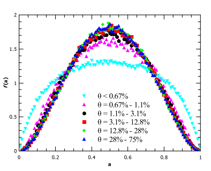
Figure 1: $f_{kMC}$ for various coverage intervals, from $\theta=0\%$ to $\theta=75\%$, for $i=1$. Between $\theta=1\%$ and $3\%$ the system has reached steady - state conditions so subsequent $f_{kMC}$ curves overlap.

To get the GSDs ($\phi_{kMC}(x)$) we used outputs at coverage $\theta=100\%$ and averaged the data over 100 runs. Every time a new island nucleated, we recorded its position within the gap and used that data to create $f_{kMC}(a)$ (as a histogram). Since we want to understand scaling properties when the steady state conditions have been achieved, we need to find the coverage at which $f_{kMC}$ stabilizes. It was previously shown in Ref. O’Neill et al. (2012) that the monomer density $n_{1}$ behaves in a manner that would yield Eqn. (3) for small gaps, but not large ones. Those findings corresponds to large coverages (where we expect to find mainly smaller gaps) versus small coverages (large gaps). Figure 1 shows $f_{kMC}$ for $i=1$, reaching steady - state condition above the coverage of approximately $\theta=1\%$.

III DFPE METHODOLOGY

For a given $f(a)$, Eqn. (2) is solved iteratively for $\phi(x)$. Following the procedure described in Ref. Mulheran et al. (2012), we perform numerical integration on a mesh of $500$ equally spaced points for $x\in[0,5]$. With an initial guess of a rectangular $\phi$, we iterate Eqn. (2) until the solution stabilizes to at least its third decimal place.

To solve the inverse problem of obtaining $f$ from a given $\phi$, we use two different strategies.

III.1 Tikhonov regularisation for the Inverse Problem

Eqn. (2) belongs to the well-known class of Fredholm integral equations of the first kind, $\phi(x)=\int k(x,a)f(a)da$, which are ill-posed. We also have an additional complication of having the left hand side $\phi(x)$ appearing in the kernel function $k(x,a)$. This means that any noise in the input data will propagate in the kernel. Hence this is not a standard inverse problem and, to the best of our knowledge, there is no established way of solving this particular type of problem. We proceed to treat Eqn. (2) as we would treat a standard Fredholm equation.

One of the most common ways to deal with ill-posed equations is the Tikhonov regularisation procedure, in which a regularisation term is added onto the original equation. This is a standard method found in many textbooks (see for example Ref. Hansen (1998)); we will describe it briefly.

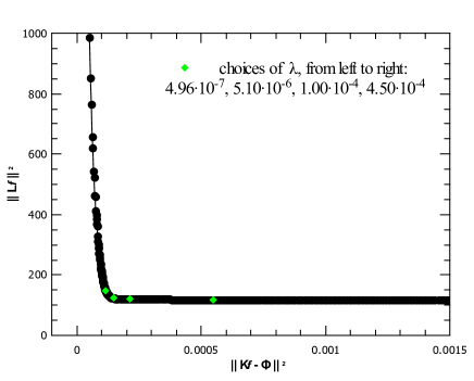
Figure 2: L-curve for inverting Eqn. (2) with $\alpha=1$ and $f$ defined by Eqn. (3). Four chosen values of $\lambda$ are marked with green diamond symbols; corresponding solutions $P_{\lambda}$ and their integrals $\phi_{\lambda}$ are shown on Figure 3.

The problem of finding $f$ that satisfies the matrix equation $Kf=\phi$ (the discretized form of Eqn. (2), where the operator $K$ stands for the kernel function and the integral operator) can be treated as a minimization problem: $\min_{f}\{\lVert Kf-\phi\rVert^{2}_{2}\}$. By adding a regularisation term this problem is substituted with: $\min_{f}\{\lVert Kf-\phi\rVert^{2}_{2}+\lambda\lVert Lf\rVert^{2}_{2}\}$. Here, $f$ is the sought solution, $L$ is the regularisation operator, usually chosen to be the identity operator or a differential operator and the regularisation parameter $\lambda>0$ controls how much weight is given to minimization of $\lVert Kf-\phi\rVert_{2}^{2}$ relative to the minimization of the added term $\lVert Lf\rVert_{2}^{2}$. Solving the inverse problem then includes choosing the appropriate operator $L$ and optimizing for $\lambda$. For a particular value of $\lambda$, the matrix equation to be solved for $f$ is:

$$(K^{T}K+\lambda L^{T}L)f_{\lambda}=K^{T}\phi$$ (4)

where $K^{T}$ is the transpose of the matrix operator $K$. It is straightforward to solve Eqn. (4) numerically.

If $K$ is ill conditioned, with an ill determined rank, the addition of the regularisation operator $L$ has a function of making Eqn. (4) well posed; then Eqn. (4) will have a unique solution $f_{\lambda}$ for all $\lambda$.

The procedure then involves solving Eqn. (4) while varying $\lambda$ to find an optimal value of $\lambda$ which stabilizes the solution without over - smoothing it. Good values of $\lambda$ are typically taken to be within the corner of the $\lVert Lf\rVert_{2}^{2}$ vs. $\lVert Kf-\phi\rVert_{2}^{2}$ plot; the so-called L-curve.

We tested the identity and the second derivative operator as candidates for the regularisation operator $L$ and, despite the fact that second derivative should be the first choice for damping oscillatory behaviour in unstable solutions, we found that we get better results when using the identity operator. In our calculations, we used routines from Ref. Press et al. (1992) (see chapter therein on Linear Regularisation Methods).

In Figures 2 and 3 (where $L$ is the identity operator), we use $f(a)=6a(1-a)$ (Equation (3) with $\alpha=1$, corresponding to the deposition case for critical island size $i=1$ or the diffusion case for $i=0$) to show the results of the Tikhonov regularisation method for a known function.

With this $f(a)$, we integrated Eqn. (2) iteratively to obtain $\phi(x)$ and solved Eqn. (4) for $f_{\lambda}$ (solved the inverse problem). Figure 2 shows the L-curve, where each point of the curve corresponds to a different $\lambda$ ($\lambda$ increases from left to the right). Note that $\lVert Kf_{\lambda}-\phi\rVert_{2}$ is the root mean error between the input $\phi$ and $\phi_{\lambda}$ (where $\phi_{\lambda}=Kf_{\lambda}$ is the result of integrating Eqn. (2) with $f=f_{\lambda}$).

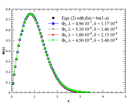
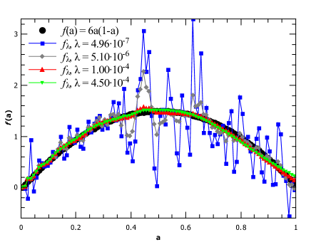
Figure 3: Top: original $\phi$ (black circles) to be inverted: the solution of integrating Eqn. (2) (where $P$ was taken to be Eqn. (3) with $\alpha=1$). After obtaining the Tikhonov results of inversion, $f_{\lambda}$, we integrated them again according to Eqn. (2) to get the shown $\phi_{\lambda}$; all of the curves overlap.
Bottom: Tikhonov results $f_{\lambda}$ ($\lambda=4.96\cdot 10^{-7}$, $5.1\cdot 10^{-6}$, $1\cdot 10^{-4}$ and $4.5\cdot 10^{-4}$), shown with the true $f(a)=6a(1-a)$ (black circles).

We chose four values of $\lambda$, highlighted on the L-curve plot, and show the four solutions $f_{\lambda}$ in Figure 3 (bottom panel), as well as the corresponding $\phi_{\lambda}$ (upper panel), alongside the original $\phi$ and $f$. While different $\phi_{\lambda}$ lie almost perfectly on top of each other and on top of input $\phi$, the solutions $f_{\lambda}$ show how strongly this problem is ill - posed. For the two smaller values of $\lambda$ the solutions $f_{\lambda}$ exhibit high oscillations and the largest $\lambda$ begins to show signs of over-smoothing in the interval $a\in[0.7,1]$. The best solution still has some noise, it isn’t symmetric, and needs normalisation; the area under the curve is $\lVert f_{\lambda}\rVert_{1}\approx 0.99$. We found that a general trend is a decreasing $\lVert\cdot\rVert_{1}$ norm with growing $\lambda$ (moving away from the corner of the L-curve to the right). The same problems are amplified when applying the method to $\phi_{kMC}$, obtained from (noisy) kMC data, with an additional problem that the solutions $f_{\lambda}$ sometimes dropped slightly below zero near $a=1$, although seemingly within the noise error we would expect when solving for kMC data input.

Since this implementation of Tikhonov regularisation doesn’t give entirely satisfactory results (loss of symmetry, $\lVert\cdot\rVert_{1}$ norm or positivity), we would need to modify it. Normalization can be always done by hand, but adding extra symmetry and positivity constraints on the regularisation, while theoretically possible, would turn the L-curve of our minimization problem into a 3-dimensional hypersurface in ${\mathbb{R}}^{4}$. This would extend the scope of work enormously so instead we look for an alternative approach.

III.2 Fourier representation for the Inverse Problem

To complement the Tikhonov regularisation results, we develop an alternative method of solving the inverse problem. In this method, we represent $f(a)$ as a finite Fourier series whose corresponding $\phi$ matches the true, kMC obtained $\phi_{kMC}$.

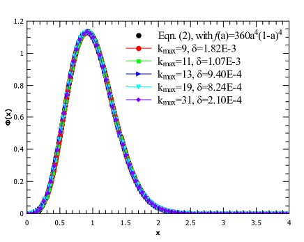
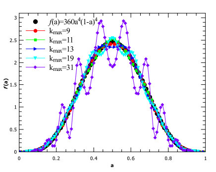
Figure 4: Searching for optimal parameter $k_{max}$: Top: original $\phi$ to be inverted (Eqn. (2) in which $f$ was taken to be Eqn. (3) with $\alpha=4$). After obtaining the results of inversion built with Fourier series, $f_{F}$, for different values of $k_{max}$, we integrated them again according to Eqn. (2) to get the $\phi_{F}$ plotted on top of each other; all of the curves overlap.
Bottom: Inversion results $f_{F}$ ($k_{max}=9$, $11$, $13$, $19$ and $31$), shown with the true $f(a)=360a^{4}(1-a)^{4}$.

Whether we take Eqn. (3) to be an accurate model of physical systems or not, $f(a)$ at least has to be equal to zero at $a=0,1$ and it is physically reasonable to assume it is symmetrical. Therefore we only use sine waves and odd wave numbers to enforce symmetry around $a=1/2$ and the requirement $f_{F}(0)=f_{F}(1)=0$. We start with a single normalized sine; $f_{F}(a)=N\sin(\pi a)$, $N$ being the normalization constant. We integrate this $f_{F}$ according to Eqn. (2) to obtain $\phi_{F}$ and calculate the error:

$$\delta=\sum_{i}(\phi_{F}(x_{i})-\phi_{kMC}(x_{i}))^{2}.$$ (5)

Then we proceed to build $f_{F}$ by adding higher random harmonics $A\sin(k\pi a)$, where in each step we randomly choose the wave number (from allowed values $k=3,5,...,k_{max}$) and the amplitude $A$ ($A\in[-A_{max},A_{max}]$), normalize the new $f_{F}$ and recalculate $\phi_{F}$ and $\delta$. Then, provided that the resulting $f_{F}$ is everywhere positive, we keep the newly added harmonic with the Boltzmann probability $\exp\left[-(\delta_{new}-\delta_{old})\beta\right]$. We repeat this cycle with a fixed $\beta$ (initially set to 1) $m$ times before increasing $\beta$ by a factor of 2 (i.e. perform a simulated anneal). After increasing $\beta$ in such a way $M$ times, we narrow in on the solution by a search in which we only keep the newly added harmonics if $\delta_{new}<\delta_{old}$.

Since there are 5 search parameters (values of $k_{max}$ and $A_{max}$, number of cycles $M,m$ and the number of search attempts while only accepting moves with $\delta_{new}<\delta_{old}$), we needed to find the optimal parameters on a known problem before proceeding to calculate $f_{F}$ for $\phi_{kMC}$.

Therefore we first integrated Eqn. (2) with $f(a)$ given by Eqn. (3), and then used the resulting $\phi$ in place of $\phi_{kMC}$ in (5), to see how can we correctly reconstruct $f_{F}$. Because Eqn. (2) is ill posed, adding higher harmonics actually leads to a worse, less stable solution $f_{F}$ with high frequency noise, as shown on Figure 4. At the same time the error $\delta$ (Eqn. (5)) can decrease (here with the rest of the search parameters fixed, although in general, when increasing $k_{max}$, a higher number of search cycles is needed to reach a stable solution). This happens regardless of the amount (or absence) of noise in the input and cannot be avoided. It is a consequence of the following property of the equation $Kf=\phi$: the inverse $K^{-1}$ of the operator $K:U\rightarrow V$ is unbounded, and the equation is ill posed, if $U$ is an infinite dimensional space Kress (2014). Hence decreasing the dimension of space, spanned with the harmonics, in which we build $f$, is a form of regularisation.

Because of that, we limited the maximum allowed wave number to 11. With $k_{max}=11$ and allowed maximum amplitude $A_{max}=0.05$ per one search attempt, we ran the simulated anneal with $m=30$ and $M=500$ cycles ($30\times 500$ random harmonic choices) and then ran through another 300 attempts, accepting only $\delta_{new}<\delta_{old}$. These are the parameters we then used to calculate $f_{F}$ for $\phi_{kMC}$, for all the values of $i$ (for $i=0$ we also use $k_{max}=5$ as explained below).

IV RESULTS

We show the diffusion and deposition $\phi$ (Eqn. (2) with $f$ given by two cases of Eqn. (3)), the GSD obtained from kMC ($\phi_{kMC}$), and $\phi_{F}$, $\phi_{\lambda}$ plotted together on upper panels in Figures 5,6,7 and 8, for critical island size $i=1,2,3$ and $0$ respectively. The solutions of integrating Eqn. (2) with $f(a)=f_{kMC}(a)$ are plotted with empty square symbols.

The bottom panels of Figures 5,6,7 and 8 show the deposition and diffusion $f(a)$ given by Equation (3), $f_{kMC}(a)$ obtained from kMC simulations, and the solutions of the inverse problem $f_{F}$ and $f_{\lambda}$.

Errors $\delta$ listed in the legends are the sum of squares differences between kMC obtained $\phi_{kMC}$ and $\phi_{F}$, $\phi_{\lambda}$ obtained by integrating the solutions $f_{F}$, $f_{\lambda}$ according to Eqn. (2) (for $\phi_{F}$ error is given with Eqn. (5) and for $\phi_{\lambda}$ with $\lVert Kf_{\lambda}-\phi_{kMC}\rVert_{2}^{2}$). The solutions $f_{F}$ are always normalized during the procedure of adding new harmonics, but the Tikhonov procedure only deals with the $\lVert\cdot\rVert_{2}$ norm so none of the $f_{\lambda}$ solutions shown have $\lVert\cdot\rVert_{1}$ norm equal to one. We have found, however, that all $i$ solutions with optimal choices of $\lambda$ have norm close to 1, and it only significantly drops (below 0.95) for too high $\lambda$ which also gave large error $\delta$.

We note here that our $f_{kMC}$ results are similar to the nucleation probabilities for $i=1$, $2$ and $3$ shown in a recent publication by González, Pimpinelli and Einstein González et al. (2017).

When we use $f_{kMC}$ to integrate Eqn. (2), the resulting GSD (empty squares in the upper panels of Figures 5, 6,7 and 8) fits the kMC obtained GSD ($\phi_{kMC}$) quite well for all the $i$ cases, but it doesn’t match it perfectly. We remind the reader here that the DFPE model we are using involves a mean field approximation; a non-mean field version suggested in Ref. Mulheran et al. (2012) gives more accurate results.

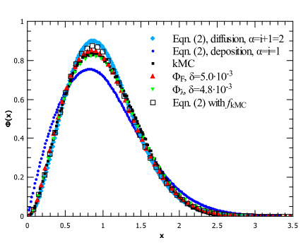
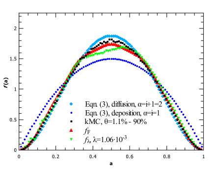
Figure 5: Critical island size $i=1$:
Top: solutions of integrating Eqn. (2) with $f$ given by Eqn. (3) ($\alpha=i+1$ case in light blue diamonds and $\alpha=i$ in dark blue circles). The kMC obtained GSD $\phi_{kMC}$ (full black squares) is inverted according to Eqn. (2); when the resulting $f_{F,\lambda}$ is used to integrate Eqn. (2) we get $\phi_{F,\lambda}$ (shown in red up and green down-facing triangles, respectively). The empty squares show the result of integrating Eqn. (2) with $f=f_{kMC}$.
Bottom: $\alpha=i+1$ and $\alpha=i$ case of Eqn. (3) (light blue diamonds and dark blue circles), the kMC result $f_{kMC}$ (full black squares) and the results of inverting $\phi_{kMC}$: $f_{F}$ (red up triangles) and $f_{\lambda}$ (green down triangles).

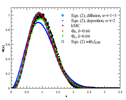
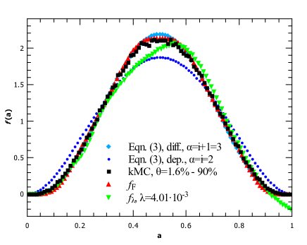
Figure 6: Critical island size $i=2$. The symbols used in this figure have the same meaning as in Fig. 5.

Returning to the inverse problem, for the $i=1$ and $2$ cases (Figures 5 and 6) both the Fourier and the Tikhonov method gave good $f_{F}$, $f_{\lambda}$ results, but in the $i=2$ case we start to see the effect of increased noise in the input $\phi_{kMC}$ relative to the $i=1$ case: $f_{\lambda}$ is noticeably negative near $a=1$. In the $i=3$ case the situation is even worse (see Figure 7), so here the Tikhonov solution is more of a guideline for the behaviour of the true $f(a)$. On the other hand, the Fourier construction was successful in all the cases so we can conclude that, by using both methods for assurance, we can find reliable solutions in problems where $f(a)$ is not directly measurable (e.g. many experiments to create nanostructures).

In the $i=0$ case (Figure 8), only the diffusion limit ($\alpha=i+1$) of Eqn. (3), as introduced in Ref. Blackman and Mulheran (1996), has physical meaning. In addition, the Fourier result for $\phi_{kMC}$ inversion with $k_{max}=11$ is problematic. Its high oscillations around $a=0.5$ suggest a higher degree of regularisation is needed, so even though the previously established cut-off $k_{max}=11$ gave excellent results when inverting Eqn. (2) for all $\alpha$ values in Eqn. (3) (including the here relevant $\alpha=i+1=1$), we additionally show the inverse $f_{F}$ where we used $k_{max}=5$. This result is backed by the Tikhonov solution ($\lambda$ is taken from the corner area of the L-curve).

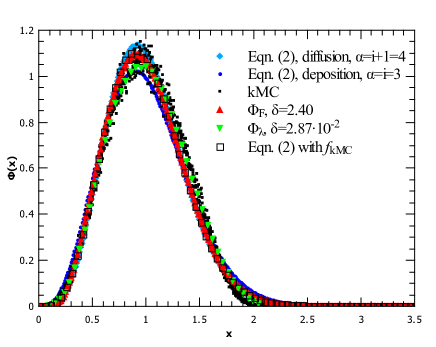
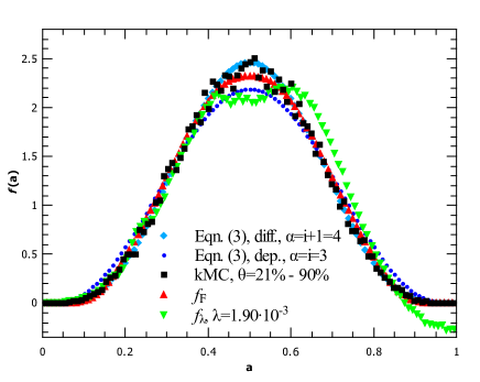
Figure 7: Critical island size $i=3$. The symbols used in this figure have the same meaning as in Fig. 5.

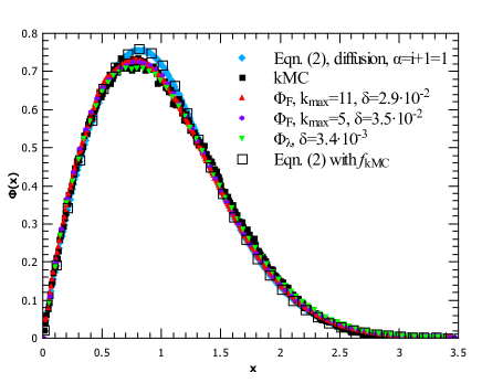
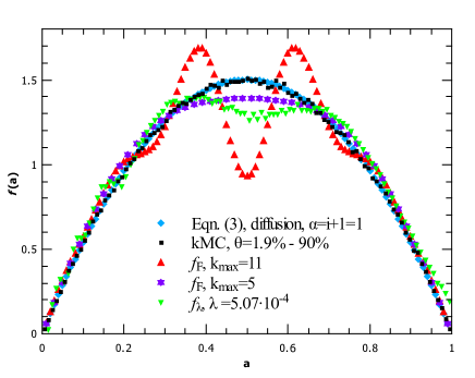
Figure 8: Critical island size $i=0$. The symbols used in this figure have the same meaning as in Fig. 5.

The measured $f_{kMC}(a)$ for $i=0$ lies almost perfectly on top of the diffusion curve. However, the solution of Eqn. (2) with $f=f_{kMC}$ is (in this case most noticeably) not matching $\phi_{kMC}$, which shows the limitations of the mean field approximation used to formulate this approach.

For critical island sizes higher than 0, the measured $f_{kMC}(a)$ (and, consequently, $\phi_{kMC}$) is at least a little below the diffusion prediction, allowing for a small contribution of the deposition driven nucleation. We finish our analysis by quantifying the level of this contribution for different $i$. Table 1 shows the result of fitting $f_{kMC}$ on a convex combination of analytic expressions for diffusion and deposition $f(a)$ from Eqn. (3):

$$f_{kMC}=\beta f_{\alpha=i+1}^{diffusion}+(1-\beta)f_{\alpha=i}^{deposition}$$ (6)

with the least squares method. We also show the fit of $\phi_{kMC}$ on the convex combination of the diffusion and deposition case,

$$\phi_{kMC}=\gamma\phi_{\alpha=i+1}^{diffusion}+(1-\gamma)\phi_{\alpha=i}^{deposition},$$ (7)

where we fitted kMC curves $\phi_{kMC}$ on the results of numerical integration of Eqn. (2). From the results, we can safely conclude that diffusion is the dominant mechanism of island nucleation. (Note that the result for $\gamma$ in the $i=2$ case is larger than 1, but not if its allowed error is subtracted.)

$i$	$\beta$	$\gamma$
1	0.821 $\pm$ 0.007	0.728 $\pm$ 0.010
2	0.819 $\pm$ 0.015	1.015 $\pm$ 0.018
3	0.844 $\pm$ 0.004	0.714 $\pm$ 0.020

Table 1: Results of fitting kMC results according to Eqns. (6) and (7).

V SUMMARY

In this paper, we have revisited the mean field DFPE (1) model of gap fragmentation on a one dimensional substrate from Ref. Mulheran et al. (2012). Using the Tikhonov regularisation method, from the kMC obtained GSD and the integral equation form of the DFPE for the GSD (Eqn. (2)) we were able to calculate the gap fragmentation probability; that is, the probability of a new island nucleation occurring at a position $a$ inside a gap ($f(a)$). The results show fair agreement with the probability $f_{kMC}(a)$ that we measured directly from kMC simulations, although they lack the expected symmetry and strict positivity. Growing amounts of numerical noise (in cases of higher $i$) aggravate this problem.

We developed an alternative method of inverting Eqn. (2) to obtain $f$, in which we represent $f$ as a finite Fourier series and use the series properties. This allows us to impose symmetry and positivity, however a downside is a more time consuming procedure due to the large amount of search parameters. The results of this method are in better agreement with the measured $f_{kMC}(a)$ so this method, especially when backed by the well - known Tikhonov method, makes for a good tool in solving problems where it is not possible to measure $f(a)$ directly.

The DFPE model we use involves two limiting cases of island nucleation: diffusion (via colliding adatoms) and deposition driven. As expected, within this framework our results (both the kMC obtained GSD and $f_{kMC}$) favour the diffusion driven nucleation as the dominant mechanism. We found no correlation between $i$ and one mechanism’s contribution amount relative to the other, however if there were a trend, a model with a built in mean field approximation would most likely be too crude for it to be observed, especially from noisy data.

Finally, we emphasize that, while the DFPE we employ here may not offer a perfect fit (as seen with the solutions of Eqn. (2) with $f_{kMC}$ which have slightly higher peaks than $\phi_{kMC}$), its strength lies in the unique possibility of calculating $f(a)$ from a given GSD, without the need for additional information.

References

- Einax et al. (2013) Mario Einax, Wolfgang Dieterich, and Philipp Maass, “Colloquium: Cluster growth on surfaces: Densities, size distributions, and morphologies,” Rev. Mod. Phys. 85, 921–939 (2013).
- Popescu et al. (2001) Mihail N. Popescu, Jacques G. Amar, and Fereydoon Family, “Rate-equation approach to island size distributions and capture numbers in submonolayer irreversible growth,” Phys. Rev. B 64, 205404 (2001).
- Mulheran and Robbie (2000) PA Mulheran and DA Robbie, “Theory of the island and capture zone size distributions in thin film growth,” EPL (Europhysics Letters) 49, 617 (2000).
- Evans and Bartelt (2002) J. W. Evans and M. C. Bartelt, “Island sizes and capture zone areas in submonolayer deposition: Scaling and factorization of the joint probability distribution,” Phys. Rev. B 66, 235410 (2002).
- Grinfeld et al. (2011) M Grinfeld, W Lamb, KP O’Neill, and PA Mulheran, “Capture-zone distribution in one-dimensional sub-monolayer film growth: a fragmentation theory approach,” Journal of Physics A: Mathematical and Theoretical 45, 015002 (2011).
- González et al. (2017) Diego Luis González, Alberto Pimpinelli, and T. L. Einstein, “Fragmentation approach to the point-island model with hindered aggregation: Accessing the barrier energy,” Phys. Rev. E 96, 012804 (2017).
- Körner et al. (2012) Martin Körner, Mario Einax, and Philipp Maass, “Capture numbers and island size distributions in models of submonolayer surface growth,” Phys. Rev. B 86, 085403 (2012).
- Gibou et al. (2003) Frédéric Gibou, Christian Ratsch, and Russel Caflisch, “Capture numbers in rate equations and scaling laws for epitaxial growth,” Phys. Rev. B 67, 155403 (2003).
- Blackman and Mulheran (1996) J. A. Blackman and P. A. Mulheran, “Scaling behavior in submonolayer film growth: A one-dimensional model,” Phys. Rev. B 54, 11681–11692 (1996).
- O’Neill et al. (2012) K. P. O’Neill, M. Grinfeld, W. Lamb, and P. A. Mulheran, “Gap-size and capture-zone distributions in one-dimensional point-island nucleation and growth simulations: Asymptotics and models,” Phys. Rev. E 85, 021601 (2012).
- Blackman et al. (2015) J.A. Blackman, M. Grinfeld, and P.A. Mulheran, “Asymptotics of capture zone distributions in a fragmentation-based model of submonolayer deposition,” Physics Letters A 379, 3146 – 3148 (2015).
- Tokar and Dreyssé (2017) VI Tokar and H Dreyssé, “Rigorous approach to fragmentation equation for irreversible epitaxial growth in the one-dimensional point island model,” Journal of Physics A: Mathematical and Theoretical 50, 375002 (2017).
- González et al. (2011) Diego Luis González, Alberto Pimpinelli, and T. L. Einstein, “Spacing distribution functions for the one-dimensional point-island model with irreversible attachment,” Phys. Rev. E 84, 011601 (2011).
- Mulheran and Blackman (1996) P. A. Mulheran and J. A. Blackman, “Capture zones and scaling in homogeneous thin-film growth,” Phys. Rev. B 53, 10261–10267 (1996).
- Fanfoni et al. (2007) M. Fanfoni, E. Placidi, F. Arciprete, E. Orsini, F. Patella, and A. Balzarotti, “Sudden nucleation versus scale invariance of InAs quantum dots on GaAs,” Phys. Rev. B 75, 245312 (2007).
- Joshi et al. (2014) Chakra P. Joshi, Yunsic Shim, Terry P. Bigioni, and Jacques G. Amar, “Critical island size, scaling, and ordering in colloidal nanoparticle self-assembly,” Phys. Rev. E 90, 032406 (2014).
- Miyamoto et al. (2009) Satoru Miyamoto, Oussama Moutanabbir, Eugene E. Haller, and Kohei M. Itoh, “Spatial correlation of self-assembled isotopically pure Ge/Si(001) nanoislands,” Phys. Rev. B 79, 165415 (2009).
- Tokar and Dreyssé (2015) V. I. Tokar and H. Dreyssé, “Universality and scaling in two-step epitaxial growth in one dimension,” Phys. Rev. E 92, 062407 (2015).
- Pimpinelli and Einstein (2007) Alberto Pimpinelli and T. L. Einstein, “Capture-zone scaling in island nucleation: Universal fluctuation behavior,” Phys. Rev. Lett. 99, 226102 (2007).
- Einstein et al. (2014) Theodore L Einstein, Alberto Pimpinelli, and Diego Luis González, “Analyzing capture zone distributions (CZD) in growth: Theory and applications,” Journal of Crystal Growth 401, 67–71 (2014), proceedings of 17th International Conference on Crystal Growth and Epitaxy (ICCGE-17).
- Groce et al. (2012) M.A. Groce, B.R. Conrad, W.G. Cullen, A. Pimpinelli, E.D. Williams, and T.L. Einstein, “Temperature-dependent nucleation and capture-zone scaling of C60 on silicon oxide,” Surface Science 606, 53 – 56 (2012).
- Potocar et al. (2011) T. Potocar, S. Lorbek, D. Nabok, Q. Shen, L. Tumbek, G. Hlawacek, P. Puschnig, C. Ambrosch-Draxl, C. Teichert, and A. Winkler, “Initial stages of a para-hexaphenyl film growth on amorphous mica,” Phys. Rev. B 83, 075423 (2011).
- Shi et al. (2009) Feng Shi, Yunsic Shim, and Jacques G. Amar, “Capture-zone areas in submonolayer nucleation: Effects of dimensionality and short-range interactions,” Phys. Rev. E 79, 011602 (2009).
- Li et al. (2010) Maozhi Li, Yong Han, and J. W. Evans, “Comment on “capture-zone scaling in island nucleation: Universal fluctuation behavior”,” Phys. Rev. Lett. 104, 149601 (2010).
- Mulheran et al. (2012) P. A. Mulheran, K. P. O’Neill, M. Grinfeld, and W. Lamb, “Distributional fixed-point equations for island nucleation in one dimension: A retrospective approach for capture-zone scaling,” Phys. Rev. E 86, 051606 (2012).
- Ratsch et al. (2005) C Ratsch, Y Landa, and R Vardavas, “The asymptotic scaling limit of point island models for epitaxial growth,” Surface science 578, 196–202 (2005).
- Hansen (1998) P. C. Hansen, Rank-Deficient and Discrete Ill-Posed Problems: Numerical Aspects of Linear Inversion, Mathematical Modeling and Computation (SIAM, Philadelphia, 1998).
- Press et al. (1992) William Hans Press, William T Vetterling, Saul A Teukolsky, and Brian P Flannery, Numerical Recipes in Fortran 77: The Art of Scientific Computing, 2nd ed. (Cambridge University Press, Cambridge, 1992).
- Kress (2014) R. Kress, Linear Integral Equations, Applied Mathematical Sciences (Springer, 2014) p. 300.