Bogoliubov Fermi surfaces: General theory, magnetic order, and topology

Abstract

We present a comprehensive theory for Bogoliubov Fermi surfaces in inversion-symmetric superconductors which break time-reversal symmetry. A requirement for such a gap structure is that the electrons posses internal degrees of freedom apart from the spin (e.g., orbital or sublattice indices), which permits a nontrivial internal structure of the Cooper pairs. We develop a general theory for such a pairing state, which we show to be nonunitary. A time-reversal-odd component of the nonunitary gap product is found to be essential for the appearance of Bogoliubov Fermi surfaces. These Fermi surfaces are topologically protected by a $\mathbb{Z}_{2}$ invariant. We examine their appearance in a generic low-energy effective model and then study two specific microscopic models supporting Bogoliubov Fermi surfaces: a cubic material with a $j=3/2$ total-angular-momentum degree of freedom and a hexagonal material with distinct orbital and spin degrees of freedom. The appearance of Bogoliubov Fermi surfaces is accompanied by a magnetization of the low-energy states, which we connect to the time-reversal-odd component of the gap product. We additionally calculate the surface spectra associated with these pairing states and demonstrate that the Bogoliubov Fermi surfaces are characterized by additional topological indices. Finally, we discuss the extension of phenomenological theories of superconductors to include Bogoliubov Fermi surfaces, and identify the time-reversal-odd part of the gap product as a composite order parameter which is intertwined with superconductivity.

I Introduction

A common view of multiband superconductivity is that the superconducting state is qualitatively like a single-band superconductor VoG85 ; SiU91 but with a momentum-dependent gap, which in particular can take on different values on different Fermi surface sheets suh59 . However, motivated in part by developments in topological materials qi11 ; sch08 ; ChS14 ; CTS16 ; ScB15 , it has recently been realized that the internal electronic degrees of freedom (i.e., orbital or sublattice) which give rise to the multiband structure can also appear in the Cooper pair wavefunction. Pairing states involving a nontrivial dependence on these internal degrees of freedom, which we refer to as “internally anisotropic” states, have been proposed for many multiband systems, such as the iron-based superconductors GSZ10 ; NGR12 ; NKT16 ; nic17 ; ong16 ; CVF16 ; agt17 , nematic superconductivity in Cu_xBi₂Se₃ CuBi2Se3 ; yon17 , $j=3/2$ pairing in cubic materials motivated by the half-Heusler compounds BWW16 ; SRV17 ; YXW17 ; RGF17 ; BoH18 ; ABT17 ; kim18 ; TSA17 , and $j=5/2$ pairing and topological superconductivity in UPt₃ NoI16 ; NoI16-2 ; yan16 . These pairing states have also attracted attention as a way to generate odd-frequency pairing bla13 ; kom15 ; LiB17 and an intrinsic ac Hall conductivity that is responsible for the polar magneto-optical Kerr effect in superconductors with broken time-reversal symmetry (TRS) tay12 ; BAA18 .

Despite this interest, an unambiguous example of an internally anisotropic pairing state has yet to be established. A key problem is that in most of the cases mentioned above, pairing states with trivial and nontrivial dependence on the internal degrees of freedom can have qualitatively the same low-energy excitation spectra. The most accessible experimental probes of unconventional superconductivity, which are sensitive only to the nodal structure of the excitation gap, thus cannot distinguish between trivial and nontrivial pairing. Indeed, the proposed experimental signatures of these exotic pairing states are quite subtle, e.g., enhanced robustness against disorder mif12 , high-energy anomalies in the density of states kom15 , the existence of the polar Kerr effect tay12 ; BAA18 , and exotic domain structures ong16 . Recently, we have shown that in one important case the consideration of internal electronic degrees of freedom leads to a unique signature in the gap structure: in clean, inversion-symmetric (even-parity) superconductors that spontaneously break TRS, the superconducting state is either fully gapped or has topologically protected Bogoliubov Fermi surfaces ABT17 . In the single-band case, the corresponding superconducting state would not have Bogoliubov Fermi surfaces but rather exhibit point or line nodes VoG85 ; SiU91 . In the multiband case, these nodes are replaced by two-dimensional Fermi surfaces by the inclusion of the internal electronic degrees of freedom. We note that Bogoliubov Fermi surfaces have been discussed for other superconductivity and superfluid systems, to which our theory does not apply. In particular, they have been proposed in strong-coupling superconductors vol89 , in superconductors and superfluids in which TRS is broken through an external effective magnetic field liu03 ; gub05 , and in superconductors and superfluids which break both TRS and inversion symmetry (IS) TSA17 ; yua18 ; vol18 .

Candidates for superconductors that break TRS have been experimentally identified through muon-spin-rotation and polar-Kerr-effect measurements, and include UPt₃ luk93 ; sch14 , Th-doped UBe₁₃ hef90 , PrOs₄Sb₁₂ aok03 ; lev18 , Sr₂RuO₄ luk98 ; xia06 , URu₂Si₂ sch15 , SrPtAs bis13 , and Bi/Ni bilayers gon16 . In addition, theory has predicted additional possibilities such as graphene nan12 ; abs14 , twisted bilayer graphene cao18-1 ; cao18-2 , the half-Heusler compound YPtBi BWW16 , water-intercalated sodium cobaltate Na_xCoO${}_{2}\cdot y$H₂O sar04 ; kie13 , Cu-doped TiSe₂ gan14 , and monolayer transition-metal dichalcogenides hsu16 . In all these cases, multiple bands either cross or come close to the Fermi surface, thus meeting the conditions for the appearance of Bogoliubov Fermi surfaces.

In this paper we present a comprehensive theory for the origins and properties of Bogoliubov Fermi surfaces. We first develop a general theory for electrons with four-valued internal degrees of freedom. Our theory is not restricted to a specific physical origin of these degrees of freedom; they could, for example, be total-angular-momentum states or a combination of a two-valued spin and a two-valued orbital degree of freedom. The normal state is assumed to be invariant under time reversal and inversion so that the spectrum generically has two doubly degenerate bands. We consider a generic, inversion-symmetric (even-parity) superconducting state that preserves IS but may break TRS. Using this theory, we establish the following results: (i) The gap is nonunitary. We define a time-reversal-odd gap product that describes the contribution to nonunitary pairing that is needed to understand the origin of the Bogoliubov Fermi surfaces. (ii) The spectrum of the Bogoliubov-de Gennes (BdG) Hamiltonian contains Bogoliubov Fermi surfaces when TRS is broken. (iii) These Bogoliubov Fermi surfaces are topologically protected by a $\mathbb{Z}_{2}$ invariant, which we give in terms of a Pfaffian. (iv) In an effective low-energy single-band model, the superconductor generates a pseudomagnetic field that is closely linked to the time-reversal-odd gap product. This pseudomagnetic field inflates point and line nodes into Bogoliubov Fermi surfaces.

We then apply this generic theory to two specific models: First, we consider cubic materials with $j=3/2$ electronic degrees of freedom, which can appear in the vicinity of the $\Gamma$ point in the Brillouin zone. In particular, we specify the pseudomagnetic fields and the associated magnetization, the structure and topology of the Bogoliubov Fermi surfaces, and the surface states that appear in the possible TRS-breaking (TRSB) superconducting states. Second, we consider hexagonal superconductors in which the internal electronic degrees of freedom stem from a two-valued spin and a two-valued orbital degree of freedom. We then turn back to a more general discussion, elucidating the topological invariants associated with Bogoliubov Fermi surfaces, using the cubic $j=3/2$ system to illustrate the results. We conclude by proposing a phenomenological Landau theory in which the magnetic and orbital order appear as an emergent composite order parameter. We speculate that the composite order could be present even if the primary superconducting order is absent, providing an example for intertwined order parameters FKT15 ; FOS18 ; BAA18 .

II General theory

Our starting point is a generic model of a fermionic system with four internal degrees of freedom that is invariant under time reversal and inversion. This model includes such important cases as two-orbital models of the pnictides RXS08 and Sr₂RuO₄ tay12 , as well as the $\Gamma_{8}$ bands of cubic materials with spin-orbit coupling L56 .

The general form of the BdG Hamiltonian reads

$$H=\frac{1}{2}\sum_{\bf k}\Psi^{\dagger}_{\bf k}{\cal H}_{\bf k}\Psi_{\bf k}\,,$$ (1)

where $\Psi_{\bf k}=(c^{T}_{\bf k},c^{\dagger}_{-{\bf k}})^{T}$ is a Nambu spinor, $c_{\bf k}$ is a four component spinor encoding the internal degrees of freedom, and the coefficient matrix is

$${\cal H}_{\bf k}=\left(\begin{array}[]{cc}H_{0}({\bf k})&\Delta({\bf k})\\ \Delta^{\dagger}({\bf k})&-H_{0}^{T}(-{\bf k})\end{array}\right).$$ (2)

The normal-state Hamiltonian $H_{0}({\bf k})$ can be written as

$${H}_{0}({\bf k})=(\epsilon_{{\bf k},0}-\mu)\,\mathbb{1}_{4}+\vec{\epsilon}_{\bf k}\cdot\vec{\gamma}\,,$$ (3)

where $\mathbb{1}_{4}$ is the $4\times 4$ unit matrix and $\vec{\gamma}=(\gamma^{1},\gamma^{2},\gamma^{3},\gamma^{4},\gamma^{5})$ is the vector of the five anticommuting Euclidean Dirac matrices. The real functions $\epsilon_{{\bf k},0}$ and $\vec{\epsilon}_{\bf k}=(\epsilon_{{\bf k},1},\epsilon_{{\bf k},2},\epsilon_{{\bf k},3},\epsilon_{{\bf k},4},\epsilon_{{\bf k},5})$ are the coefficients of these matrices and $\mu$ is the chemical potential. We make the simplifying assumption that IS $P$ acts trivially on the internal degrees of freedom so that the coefficients in Eq. (3) are even functions of momentum. Time reversal is implemented by $T={\cal K}U_{T}$, where ${\cal K}$ is complex conjugation and the unitary part can be chosen, without loss of generality, as $U_{T}=\gamma^{1}\gamma^{2}$. The invariance of the normal-state Hamiltonian under time reversal then implies that $\gamma^{1}$ and $\gamma^{2}$ are both imaginary, and the other three matrices are real.

The normal-state Hamiltonian in Eq. (3) has the doubly degenerate eigenvalues $E_{{\bf k},\pm}-\mu$, where

$$E_{{\bf k},\pm}=\epsilon_{{\bf k},0}\pm|\vec{\epsilon}_{\bf k}|\,.$$ (4)

Due to the presence of IS and TRS, we can distinguish the two states corresponding to each eigenvalue by a pseudospin index $s=\pm 1$. The pseudospin-$s$ state $|{\bf k},\pm,s\rangle$ in the $\pm$ band at momentum ${\bf k}$ then transforms as

$$P\,|{\bf k},\pm,s\rangle =|{-}{\bf k},\pm,s\rangle\,,$$ (5)

$$T\,|{\bf k},\pm,s\rangle =-s\,|{-}{\bf k},\pm,-s\rangle\,.$$ (6)

Although the pseudospin basis only needs to satisfy these two criteria, it is nevertheless often possible to choose the basis such that the pseudospin index transforms like a true spin $1/2$ under the symmetries of the lattice, a so-called manifestly covariant Bloch basis (MCBB) F15 . In Appendix A, we present choices of MCBBs for the two model systems considered in the rest of the paper. We note, however, that the analysis in this section requires only that Eqs. (5) and (6) are satisfied.

Topologically stable Bogoliubov Fermi surfaces only appear for inversion-symmetric superconducting states. The pairing potential consistent with this has the general form

$${\Delta}({\bf k})=\eta_{{\bf k},0}\,U_{T}+\vec{\eta}_{\bf k}\cdot\vec{\gamma}\,U_{T}\,,$$ (7)

where the pairing amplitudes $\eta_{{\bf k},0}$ and $\vec{\eta}_{\bf k}=(\eta_{{\bf k},1},\eta_{{\bf k},2},\eta_{{\bf k},3},\eta_{{\bf k},4},\eta_{{\bf k},5})$ are even functions of momentum. The first term in Eq. (7) describes standard pairing between time-reversed states. This we call “internally isotropic” pairing to describe how the underlying electronic degrees of freedom are paired. The second term describes pairing in the five “internally anisotropic” channels, where the electronic degrees of freedom in the Cooper pair do not generally come from Kramers partners. In general, these pairing states transform nontrivially under lattice symmetries due to their dependence on the internal degrees of freedom. The pairing potential breaks TRS if the coefficients $\eta_{{\bf k},0}$ and $\vec{\eta}_{\bf k}$ cannot be chosen as real, up to a common and momentum-independent phase factor.

Expressed in the pseudospin basis where the annihilation operator has the spinor form $\tilde{c}_{\bf k}^{T}=(c_{{\bf k},+,\uparrow},c_{{\bf k},+,\downarrow},c_{{\bf k},-,\uparrow},c_{{\bf k},-,\downarrow})$, the pairing Hamiltonian reads

$$\tilde{\Delta}({\bf k})=\left(\begin{array}[]{cc}\psi_{{\bf k},+}\,i{s}_{y}&(\psi_{{\bf k},I}{s_{0}}+i{\bf d}_{\bf k}\cdot{\bf s})\,i{s}_{y}\\ (\psi_{{\bf k},I}{s_{0}}-i{\bf d}_{\bf k}\cdot{\bf s})\,i{s}_{y}&\psi_{{\bf k},-}\,i{s}_{y}\end{array}\right),$$ (8)

where $\mathbf{s}=(s_{x},s_{y},s_{z})$ is the vector of Pauli matrices and $s_{0}$ is the unit matrix in pseudospin space and all functions in the matrix are even in momentum. The intraband pseudospin-singlet pairing potentials on the diagonal have the basis-independent form

$$\psi_{{\bf k},\pm}=\eta_{{\bf k},0}\pm\frac{\vec{\epsilon}_{\bf k}\cdot\vec{\eta}_{\bf k}}{|\vec{\epsilon}_{\bf k}|}\,.$$ (9)

The off-diagonal blocks describe unconventional interband pairing, with both pseudospin singlet and triplet potentials, $\psi_{{\bf k},I}$ and ${\bf d}_{\bf k}$, respectively. While the form of the interband pairing potentials depends on the choice of pseudospin basis in each band, these potentials must satisfy

$$|\psi_{{\bf k},I}|^{2}+|{\bf d}_{\bf k}|^{2}=|\vec{\eta}_{\bf k}|^{2}-\frac{|\vec{\epsilon}_{\bf k}\cdot\vec{\eta}_{\bf k}|^{2}}{|\vec{\epsilon}_{\bf k}|^{2}}\,.$$ (10)

The interband terms involve only the internally anisotropic pairing channels, as the pairing of time-reversed partners in the conventional state (i.e., the internally isotropic pairing) implies a purely intraband potential. Note that the sign change between the pseudospin triplet potentials in the off-diagonal blocks of Eq. (8) is required by fermionic antisymmetry; the factor of $i$ ensures that ${\bf d}$ is a real vector in the case of a time-reversal-symmetric pairing state.

x

II.1 Nonunitary pairing and time-reversal-odd gap product

The presence of the five internally anisotropic pairing channels in our model generically implies that the pairing is nonunitary. That is, the product $\Delta({\bf k})\Delta^{\dagger}({\bf k})$ is not proportional to the unit matrix, but is instead given by

$$\Delta({\bf k})\Delta^{\dagger}({\bf k}) =\left(|\eta_{{\bf k},0}|^{2}+|\vec{\eta}_{\bf k}|^{2}\right)\mathbb{1}_{4}+2\,\text{Re}(\eta^{\ast}_{{\bf k},0}\vec{\eta}_{\bf k})\cdot\vec{\gamma}$$

$$\quad{}+\sum_{n>m>0}2i\,\text{Im}(\eta_{{\bf k},n}\eta_{{\bf k},m}^{\ast})\,\gamma^{n}\gamma^{m}\,.$$ (11)

The first term on the right-hand side represents the unitary part of the gap product, while the next two terms constitute the nonunitary part. The first of these appears when pairing occurs in both the internally isotropic and internally anisotropic pairing channels and does not require the breaking of any symmetry. The second nonunitary term is only present in a TRSB state with a nontrivial phase difference between at least two internally anisotropic channels. As we shall see below, only the latter term is relevant for the appearance of the Bogoliubov Fermi surfaces. For later reference, we also give the gap product in the pseudospin basis,

$$\tilde{\Delta}({\bf k})\tilde{\Delta}^{\dagger}({\bf k})=\left[\frac{1}{2}\left(|\psi_{{\bf k},+}|^{2}+|\psi_{{\bf k},-}|^{2}\right)+|\psi_{{\bf k},I}|^{2}+|{\bf d}_{\bf k}|^{2}\right]\mathbb{1}$$

$${}+\left(\begin{array}[]{cc}\tfrac{1}{2}(|\psi_{{\bf k},+}|^{2}-|\psi_{{\bf k},-}|^{2})s_{0}+(i{\bf d}_{\bf k}\times{\bf d}^{\ast}_{\bf k}+2\,\text{Im}(\psi_{{\bf k},I}{\bf d}^{\ast}_{\bf k}))\cdot{\bf s}&(\psi_{{\bf k},+}\psi^{\ast}_{{\bf k},I}+\psi_{{\bf k},-}^{\ast}\psi_{{\bf k},I})s_{0}+i(\psi_{{\bf k},+}{\bf d}^{\ast}_{\bf k}+\psi_{{\bf k},-}^{\ast}{\bf d}_{\bf k})\cdot{\bf s}\\ (\psi_{{\bf k},-}\psi^{\ast}_{{\bf k},I}+\psi_{{\bf k},+}^{\ast}\psi_{{\bf k},I})s_{0}-i(\psi_{{\bf k},+}^{\ast}{\bf d}_{\bf k}+\psi_{{\bf k},-}{\bf d}^{\ast}_{\bf k})\cdot{\bf s}&\tfrac{1}{2}(|\psi_{{\bf k},-}|^{2}-|\psi_{{\bf k},+}|^{2})s_{0}+(i{\bf d}_{\bf k}\times{\bf d}^{\ast}_{\bf k}-2\,\text{Im}(\psi_{{\bf k},I}{\bf d}^{\ast}_{\bf k}))\cdot{\bf s}\end{array}\right).$$ (14)

The diagonal blocks of the nonunitary part will play an important role later, in particular the terms involving the pseudospin vector ${\bf s}$. Since these terms only depend on the interband pairing potentials in Eq. (8), they arise from the last term in Eq. (11) and hence require TRSB pairing in different internally anisotropic channels.

To gain insight into the physical meaning of the nonunitary gap and its relation to broken TRS, we briefly review the more familiar case of nonunitary pairing in a single band of spin-$1/2$ electrons SiU91 . Here it is customary to write the gap function as $\Delta_{\bf k}=(\psi_{\bf k}+{\bf d}_{\bf k}\cdot\bm{\sigma})\,i\sigma_{y}$, where $\psi_{\bf k}$ is the singlet pairing potential, ${\bf d}_{\bf k}$ describes triplet pairing, and $\bm{\sigma}$ is the vector of spin Pauli matrices. The gap product is then

$$\Delta_{\bf k}\Delta_{\bf k}^{\dagger} =(|\psi_{\bf k}|^{2}+|{\bf d}_{\bf k}|^{2})\,\sigma_{0}+2\,\text{Re}(\psi_{\bf k}{\bf d}^{\ast}_{\bf k})\cdot\bm{\sigma}$$

$$\quad{}+i\,({\bf d}_{\bf k}\times{\bf d}^{\ast}_{\bf k})\cdot\bm{\sigma}\,.$$ (15)

The presence of either of the last two terms indicates a nonunitary gap, which requires the breaking of IS or TRS, respectively. The presence of the nonunitary part of the gap product indicates a nonzero value of the spin polarization $\operatorname{Tr\,}(\Delta_{\bf k}^{\dagger}\bm{\sigma}\Delta_{\bf k})$ of the pairing state at ${\bf k}$. This spin polarization has two contributions, one that breaks TRS and one that does not. The latter is a consequence of broken IS and typically the associated spin polarization is already present in the normal state smi17 . The spin polarization due to broken TRS does not exist in the normal state but appears spontaneously in the TRSB superconducting state and is usually taken as the defining characteristic of nonunitary pairing SiU91 . Below we will define a time-reversal-odd gap product that isolates this contribution, refining the meaning of nonunitary pairing.

Returning to our four-component system, the nonunitary part of the gap product in Eq. (11) can be similarly interpreted as a polarization of the internal degrees of freedom in the pairing state. Moreover, the terms proportional to the pseudospin Pauli matrices in the diagonal blocks of Eq. (14) may also be interpreted as the pseudospin polarization $\operatorname{Tr\,}[\Delta^{\dagger}({\bf k}){\cal P}_{{\bf k},\pm}\check{\bf s}{\cal P}_{{\bf k},\pm}\Delta({\bf k})]$ of the pairing state in the $\pm$ band, where ${\cal P}_{{\bf k},\pm}$ are projection operators on the normal-state Hilbert space which project onto the $\pm$ bands at momentum ${\bf k}$ and

$$\check{\bf s}\equiv\left(\begin{array}[]{cc}{\bf s}&0\\ 0&{\bf s}\end{array}\right).$$ (16)

We thus expect a nonvanishing pseudospin polarization of the low-energy states in our model. As in the single-band case discussed above, there will be a contribution to this pseudospin polarization that is due solely to the spontaneous breaking of TRS in the superconducting state. In the next paragraph we discuss how to identify its origin.

To link more closely to broken TRS, it is useful to refine the notion of the nonunitary portion of the gap product and define a time-reversal-odd gap product. The time-reversal operator expressed in the Nambu basis is $T={\cal K}U_{T}\tau_{0}$, where $\tau_{0}$ is the unit matrix in particle-hole space. Time reversal operates as

$${\cal H}_{\bf k}\rightarrow(\tau_{0}U_{T}){\cal H}^{*}_{-\bf k}(\tau_{0}U_{T})^{\dagger}\,.$$ (17)

From this expression, the form of the gap function, and $U_{T}=\gamma^{1}\gamma^{2}$, we find the key and natural result that the gap function transforms as

$$\Delta({\bf k})\rightarrow\Delta_{T}({\bf k})\equiv U_{T}\Delta^{*}({\bf-k})U_{T}^{\dagger}=(\eta^{*}_{{\bf k},0}+\vec{\eta}_{\bf k}^{*}\cdot\vec{\gamma})\,U_{T}\,.$$ (18)

Similarly, under time reversal the gap product transforms as

$$\Delta({\bf k})\Delta^{\dagger}({\bf k})\rightarrow U_{T}\Delta^{*}(-{\bf k})\Delta^{T}(-{\bf k})U_{T}^{\dagger}=\Delta_{T}({\bf k}){\Delta}_{T}^{\dagger}({\bf k})\,.$$ (19)

This justifies the following time-reversal-odd gap product as a measure of broken TRS:

$$\Delta({\bf k}) \Delta^{\dagger}({\bf k})-\Delta_{T}({\bf k})\Delta_{T}^{\dagger}({\bf k})$$

$$=(\vec{\eta}_{\bf k}\cdot\vec{\gamma})(\vec{\eta}_{\bf k}^{*}\cdot\vec{\gamma})-(\vec{\eta}_{\bf k}^{*}\cdot\vec{\gamma})(\vec{\eta}_{\bf k}\cdot\vec{\gamma})$$

$$=\sum_{i,j}(\eta_{i}\eta_{j}^{*}-\eta_{i}^{*}\eta_{j})\,\gamma_{i}\gamma_{j}\,,$$ (20)

which yields the time-reversal-odd contribution to Eq. (11). Applying the same analysis to the gap function $\Delta_{\bf k}=(\psi_{\bf k}+{\bf d}_{\bf k}\cdot\bm{\sigma})\,i\sigma_{y}$ of the single-band model, the time-reversal-odd gap product is

$$\Delta_{\bf k}\Delta_{\bf k}^{\dagger}-\sigma_{y}\Delta^{\ast}_{-\bf k}\Delta^{T}_{-\bf k}\sigma_{y}=2i\,({\bf d}_{\bf k}\times{\bf d}_{\bf k}^{*})\cdot\bm{\sigma}\,,$$ (21)

yielding the term that is usually taken to define a nonunitary superconductor SiU91 . Finally, if the time-reversal-odd gap product is calculated for the gap function expressed in the pseudospin basis, Eq. (8), then the terms proportional to the pseudospin Pauli matrices in the diagonal blocks of Eq. (14) are the only terms that remain in these blocks. As mentioned earlier, these terms play a central role in the effective low-energy model.

II.2 Bogoliubov Fermi surfaces

The BdG Hamiltonian in Eq. (2) possesses both particle-hole symmetry $C$ and IS $P$. Particle-hole symmetry dictates that

$$U_{C}{\cal H}_{-{\bf k}}^{\ast}U_{C}^{\dagger}=-{\cal H}_{{\bf k}}\,,$$ (22)

where the unitary part is $U_{C}=\tau_{x}\otimes\mathbb{1}_{4}$ and $\tau_{i}$ are the Pauli matrices in particle-hole space. Inversion acts as

$$U_{P}{\cal H}_{-{\bf k}}U_{P}^{\dagger}={\cal H}_{{\bf k}}\,,$$ (23)

where $U_{P}=\tau_{0}\otimes\mathbb{1}_{4}$. The product of these symmetries thus gives

$$U_{CP}{\cal H}_{{\bf k}}^{\ast}U^{\dagger}_{CP}=-{\cal H}_{{\bf k}}\,,$$ (24)

where $U_{CP}=U_{C}U_{P}^{\ast}=\tau_{x}\otimes\mathbb{1}_{4}$. It hence follows that $(CP)^{2}=+1$. The existence of this $CP$ symmetry and the property that it squares to unity guarantees that the BdG Hamiltonian can be unitarily transformed into an antisymmetric matrix ABT17 . For example, defining

$$\tilde{\cal H}_{\bf k}=\Omega{\cal H}_{\bf k}\Omega^{\dagger}\,,$$ (25)

where

$$\Omega=\frac{1}{\sqrt{2}}\left(\begin{array}[]{cc}1&1\\ i&-i\end{array}\right)\otimes\mathbb{1}_{4}\,,$$ (26)

we find that $\tilde{\cal H}^{T}_{\bf k}=-\tilde{\cal H}_{\bf k}$. We can then evaluate the Pfaffian of this matrix, which is given in compact form by

$$P({\bf k})=\text{Pf}\>\tilde{\cal H}_{\bf k} =\big{(}\langle\underline{\epsilon}_{\bf k},\underline{\epsilon}_{\bf k}\rangle-\langle\underline{\eta}_{\bf k},\underline{\eta}^{\ast}_{\bf k}\rangle\big{)}^{2}+4\,\big{|}\langle\underline{\epsilon}_{\bf k},\underline{\eta}_{\bf k}\rangle\big{|}^{2}\quad$$

$$\quad{}+\langle\underline{\eta}_{\bf k},\underline{\eta}_{\bf k}\rangle\langle\underline{\eta}^{\ast}_{\bf k},\underline{\eta}^{\ast}_{\bf k}\rangle-\langle\underline{\eta}_{\bf k},\underline{\eta}^{\ast}_{\bf k}\rangle^{2}\,,$$ (27)

where we adopt the “six-vector” notation

$$\underline{\epsilon}_{\bf k}=(\epsilon_{{\bf k},0}{-}\mu,\vec{\epsilon}_{\bf k})\,,\quad\underline{\eta}_{\bf k}=(\eta_{{\bf k},0},\vec{\eta}_{\bf k})\,,$$ (28)

and define $\langle\underline{a},\underline{b}\rangle=a_{0}b_{0}-\vec{a}\cdot\vec{b}$.

Prior to examining the Pfaffian of Eq. (27), it is useful to consider the case of a single-band model to highlight the new physics that result from Eq. (27). In particular, for a single-band system that is inversion and time-reversal invariant in the normal state and retains IS in the superconducting state, the BdG Hamiltonian takes the usual pseudospin-singlet form

$${\cal H}_{\bf k}=\left(\begin{array}[]{cc}\xi_{0}({\bf k})\,\sigma_{0}&\psi({\bf k})\,i\sigma_{2}\\ -\psi^{*}({\bf k})\,i\sigma_{2}&-\xi_{0}({\bf k})\,\sigma_{0}\end{array}\right).$$ (29)

Using the same arguments leading to Eq. (27), the Pfaffian for Eq. (29) is simply

$$\text{Pf}\>{\cal H}_{\bf k}=\xi_{0}^{2}({\bf k})+|\psi({\bf k})|^{2}\,.$$ (30)

Notice that this expression is always nonnegative and only vanishes when (i) ${\bf k}$ is on the Fermi surface, where $\xi_{0}({\bf k})=0$, and (ii) the gap vanishes, $\psi({\bf k})=0$. Since zeros of the Pfaffian give the zeros of the excitation spectrum, these two conditions immediately imply that Bogoliubov Fermi surfaces generically do not appear in single-band systems, where only point and line nodes are expected SiU91 .

In general, Hamiltonians with $(CP)^{2}=+1$ can possess Fermi surfaces with a nontrivial $\mathbb{Z}_{2}$ topological charge KST14 ; ZSW16 ; ABT17 . That is, they are stable against any $CP$-preserving perturbation. The $\mathbb{Z}_{2}$ invariant is defined in Ref. ABT17 in terms of the Pfaffian in Eq. (27) as

$$(-1)^{l}=\text{sgn}\,[P({\bf k}_{-})P({\bf k}_{+})]\,,$$ (31)

where ${\bf k}_{-}$ (${\bf k}_{+}$) refers to momenta inside (outside) the Fermi surface, which is characterized by $P({\bf k})=0$. Fermi surfaces with $l=1$ are topologically nontrivial, as there must necessarily be a surface of zeros of the Pfaffian separating regions where it has opposite sign. In contrast, Fermi surfaces with $l=0$ are not topologically protected and can be removed by a $CP$-preserving perturbation.

One easily sees from Eq. (27) that the Pfaffian is always nonnegative in the absence of superconductivity, i.e., for $\underline{\eta}_{\bf k}=(0,\vec{0})$. This reflects the fact that the normal-state Fermi surfaces, given by the zeros of $\langle\underline{\epsilon}_{\bf k},\underline{\epsilon}_{\bf k}\rangle=E_{{\bf k},+}E_{{\bf k},-}$, can be gapped out by the superconductivity, which preserves IS and particle-hole symmetry. Superconducting states which preserve TRS, where one can choose a gauge such that $\underline{\eta}_{\bf k}=\underline{\eta}^{\ast}_{\bf k}$, also yield a nonnegative Pfaffian, as the last line of Eq. (27) then vanishes. Since the Pfaffian is defined locally in momentum space, this argument also holds for any TRSB state defined by a single momentum-dependent phase, i.e., where the pairing satisfies $\underline{\eta}_{\bf k}=\underline{\eta}^{r}_{\bf k}\,e^{i\phi_{\bf k}}$ with $\underline{\eta}^{r}_{\bf k}$ entirely real. Notice also that when the superconductor is time-reversal invariant the nodes generally do not lie on the Fermi surface, in contrast to the single-band case. This follows by observing that for momenta on the Fermi surface $\langle\underline{\epsilon}_{\bf k},\underline{\epsilon}_{\bf k}\rangle=E_{{\bf k},+}E_{{\bf k},-}=0$ so that $P({\bf k})=4|\langle\underline{\epsilon}_{\bf k},\underline{\eta}_{\bf k}\rangle|^{2}\neq 0$. The position of nodes can therefore change as the parameters in the Hamiltonian are changed, allowing for the possibility of annihilating nodes, which has been argued to be relevant to monolayer FeSe nic17 ; CVF16 ; agt17 .

The last term of the Pfaffian is only nonzero if there is pairing in multiple superconducting channels with nontrivial phase difference between them. Writing the pairing potential in each channel as $\eta_{{\bf k},n}=|\eta_{{\bf k},n}|\,e^{i\phi_{{\bf k},n}}$, the last line of Eq. (27) is then

$$\langle\underline{\eta}_{\bf k} ,\underline{\eta}_{\bf k}\rangle\langle\underline{\eta}^{\ast}_{\bf k},\underline{\eta}^{\ast}_{\bf k}\rangle-\langle\underline{\eta}_{\bf k},\underline{\eta}^{\ast}_{\bf k}\rangle^{2}$$

$$=2\sum_{n>0}|\eta_{{\bf k},0}|^{2}|\eta_{{\bf k},n}|^{2}\big{[}1-\cos(2[\phi_{{\bf k},0}-\phi_{{\bf k},n}])\big{]}$$

$$\quad{}-2\!\sum_{n>m>0}\!|\eta_{{\bf k},n}|^{2}|\eta_{{\bf k},m}|^{2}\big{[}1-\cos(2[\phi_{{\bf k},n}-\phi_{{\bf k},m}])\big{]}\,.$$ (32)

The first term on the right-hand side shows that coexisting internally isotropic and internally anisotropic channels always give a nonnegative contribution to the Pfaffian. In contrast, coexisting internally anisotropic channels give a nonpositive contribution, which is strictly negative if the relative phase differences between the unconventional channels break TRS. This is the only way to obtain a negative Pfaffian and thus topologically stable Bogoliubov Fermi surfaces. It is also equivalent to the presence of a non-vanishing time-reversal-odd gap product in Eq. (20), and thus to a nonvanishing pseudospin polarization.

We now explicitly demonstrate that the Pfaffian can be negative and hence that Bogoliubov Fermi surfaces exist. To simplify the discussion, we consider a TRSB state that only involves the internally ansiotropic pairing channels. Nodes are expected to occur on the normal-state Fermi surface where the intraband pairing potential vanishes, i.e., where $\vec{\epsilon}_{\bf k}\cdot\vec{\eta}_{\bf k}=0$, see Eq. (9). If $\vec{\eta}_{\bf k}$ is real up to an overall phase factor, which corresponds to the time-reversal-symmetric case, this equation describes a surface in the Brillouin zone. On the other hand, if $\vec{\eta}_{\bf k}$ has irreducible real and imaginary parts, corresponding to the TRSB case, this equation generically decomposes into two independent real equations and thus describes a line. Restricting ourselves to momenta where this condition is satisfied, the Pfaffian has the simpler form

$$P({\bf k}) =(E_{{\bf k},+}E_{{\bf k},-}+|\vec{\eta}_{\bf k}|^{2})^{2}$$

$${}-2\sum_{n>m>0}|\eta_{{\bf k},n}|^{2}|\eta_{{\bf k},m}|^{2}\left[1-\cos(2[\phi_{{\bf k},n}-\phi_{{\bf k},m}])\right].$$ (33)

The product $E_{{\bf k},+}E_{{\bf k},-}$ changes sign on the normal-state Fermi surface. For sufficiently small $|\vec{\eta}_{\bf k}|$, it is therefore possible to find a point in momentum space close to the normal-state Fermi surface, where the first term in Eq. (33) vanishes. The Pfaffian will then be negative if the second line is nonzero, which is always true for a nonunitary TRSB state as long as $\vec{\eta}_{\bf k}\neq 0$. That is, the node must arise from the projection of the internally anisotropic states onto the Fermi surface, and not be intrinsic to the internally ansiotropic pairing potentials $\vec{\eta}_{\bf k}$ themselves. Since far away from the Fermi surface the product $E_{{\bf k},+}E_{{\bf k},-}$ should dominate over the terms involving the gap, there will also be a region in the Brillouin zone where the Pfaffian is positive. We thus deduce the existence of a topologically stable Bogoliubov Fermi surface forming the boundary between the regions of positive and negative Pfaffian.

II.3 Effective low-energy model

Further insight into the appearance of Bogoliubov Fermi surfaces can be obtained from an effective single-band model valid for the states close to the normal-state Fermi surface. In deriving this model, we make the weak-coupling assumption that, on the Fermi surface of each band, the direct energy gap separating the two bands is much larger than the pairing potential, i.e., $|E_{{\bf k},+}-E_{{\bf k},-}|=2|\vec{\epsilon}_{\bf k}|\gg\max(|\eta_{{\bf k},0}|,|\vec{\eta}_{\bf k}|)$.

Without loss of generality, we assume that the $-$ band intersects the Fermi energy. The Green function $G_{-}({\bf k},\omega)$ of the states in the $-$ band satisfies

$$G_{-}^{-1}({\bf k},\omega)=\omega-H_{{\bf k},-}-H_{{\bf k},I}^{\dagger}(\omega-H_{{\bf k},+})^{-1}H_{{\bf k},I}\,,$$ (34)

where $H_{{\bf k},\pm}$ and $H_{{\bf k},I}$ are blocks of the BdG Hamiltonian transformed into the pseudospin basis,

$$\tilde{\cal H}=\left(\begin{array}[]{cc}H_{{\bf k},+}&H_{{\bf k},I}\\[2.15277pt] H^{\dagger}_{{\bf k},I}&H_{{\bf k},-}\end{array}\right).$$ (35)

Note that $H_{{\bf k},I}$ describes the interband coupling due to superconductivity in the internally anisotropic channels.

To lowest order in the pairing potential, an effective model is obtained by ignoring the last term in Eq. (34), which simply gives the projection of the Hamiltonian onto the low-energy states. This describes pseudospin-singlet pairing in a doubly degenerate single band and does not yield the Bogoliubov Fermi surfaces. To obtain the leading correction to the projected Hamiltonian, we analyze the last term in Eq. (34). Since we are interested in the low-energy states in the $-$ band, we approximate $\omega\approx 0$ in this term. Furthermore, as the $+$ band is assumed to lie far from the Fermi surface, we can ignore the effect of the pairing on its dispersion, i.e., we can write $H_{{\bf k},+}\approx(E_{{\bf k},+}-\mu)\,{s_{0}}\tau_{z}$, where $\tau_{z}$ is a Pauli matrix in Nambu space. Using the fact that $E_{{\bf k},-}\approx\mu$ close to the Fermi surface of the $-$ band, we hence make the replacement

$$(\omega-H_{{\bf k},+})^{-1}\approx(E_{{\bf k},-}-E_{{\bf k},+})^{-1}\,{s_{0}}\tau_{z}=-\frac{1}{2|\vec{\epsilon}_{\bf k}|}\,{s_{0}}\tau_{z}\,.$$ (36)

Inserting this into Eq. (34), we obtain the effective Hamiltonian

$$H^{\text{eff}}_{{\bf k},-}=H_{{\bf k},-}+\delta H_{{\bf k},-}\,,$$ (37)

with the correction term

$$\delta H_{{\bf k},-}=-\frac{1}{2|\vec{\epsilon}_{\bf k}|}\,H_{{\bf k},I}^{\dagger}\tau_{z}H_{{\bf k},I}$$

$$=\left(\begin{array}[]{cc}\delta\epsilon_{{\bf k},-}s_{0}+\delta{\bf h}_{{\bf k},-}\cdot{\bf s}&0\\ 0&-\delta\epsilon_{{\bf k},-}s_{0}-\delta{\bf h}_{{\bf k},-}\cdot{\bf s}^{T}\end{array}\right),$$ (40)

where

$$\delta\epsilon_{{\bf k},-} =\frac{|\psi_{{\bf k},I}|^{2}+|{\bf d}_{\bf k}|^{2}}{2\,|\vec{\epsilon}_{\bf k}|}\,,$$ (41)

$$\delta{\bf h}_{{\bf k},-} =\frac{i{\bf d}_{\bf k}\times{\bf d}_{\bf k}^{\ast}-2\,\text{Im}(\psi_{{\bf k},I}{\bf d}_{\bf k}^{\ast})}{2\,|\vec{\epsilon}_{\bf k}|}$$

$$=-\frac{\operatorname{Tr\,}[{\Delta}^{\dagger}({\bf k}){\cal P}_{{\bf k},-}\check{\bf s}{\cal P}_{{\bf k},-}{\Delta}({\bf k})]}{4\,|\vec{\epsilon}_{\bf k}|}\,.$$ (42)

The term $\delta\epsilon_{{\bf k},-}$ modifies the dispersion and is always present when there is interband pairing. The term $\delta{\bf h}_{{\bf k},-}\cdot{\bf s}$ is more interesting: It describes an effective “pseudomagnetic” field, which is proportional to the pseudospin polarization of the band states in a nonunitary state. It is hence only present in TRSB states where the unconventional channels have nontrivial relative phase differences. It directly leads to the appearance of Bogoliubov Fermi surfaces, as can be seen in the eigenvalue spectrum of the low-energy effective model,

$$\pm|\delta{\bf h}_{{\bf k},-}|\pm\sqrt{(E_{{\bf k},-}+\delta\epsilon_{{\bf k},-}-\mu)^{2}+|\psi_{{\bf k},-}|^{2}}\>,$$ (43)

where the two $\pm$ signs are chosen independently. If the pseudomagnetic field is nonzero at a node of the intraband pairing potential $\psi_{{\bf k},-}$, the dispersion is split and shifted to finite energies, leading to Bogoliubov Fermi surfaces. Since $\delta{\bf h}_{{\bf k},-}$ is proportional to the product of the internally anisotropic pairing potentials, it is therefore necessary that these potentials are nonzero at the node, consistent with the condition found above that the node is due to the projection into the low-energy states.

We note that the modification of the normal-state dispersion by $\delta\epsilon_{{\bf k},-}$ can have a nontrivial effect on the electronic structure of the superconducting state even when TRS is not broken. Specifically, as also discussed above for the general theory, line nodes arising from the projection of the pairing potential onto the band basis, i.e., for which $\vec{\epsilon}_{\bf k}\cdot\vec{\eta}_{\bf k}=0$ but $\vec{\eta}_{\bf k}=0$, are shifted off the normal-state Fermi surface by $\delta\epsilon_{{\bf k},-}$, so that they instead occur on the surface defined by $E_{{\bf k},-}+\delta\epsilon_{{\bf k},-}=\mu$, allowing for pairs of nodes to annihilate nic17 ; CVF16 ; agt17 .

III Cubic superconductors

In this section, we consider superconductivity in the $\Gamma_{8}$ bands of a cubic system as the first concrete example of the generic model studied above. Here, the four internal degrees of freedom of the electrons reflect their total angular momentum $j=3/2$, which arises from the strong atomic spin-orbit coupling. We present a tight-binding generalization of the Luttinger-Kohn model of the $\Gamma_{8}$ bands for the point group $O_{h}$ L56 . Our strategy is to take the simplest nontrivial model that is consistent with the imposed symmetries. In this spirit, we restrict ourselves to nearest-neighbor hopping on the fcc lattice and only consider local Cooper pairing. We determine the Bogoliubov Fermi surfaces and examine the associated nonunitary gap structure both in the $j=3/2$ basis and in the pseudospin basis near the Fermi surface.

The $j=3/2$ effective spin of the electrons in the cubic superconductor implies that the Nambu spinor in Eq. (1) is $\Psi_{\mathbf{k}}=(c_{\mathbf{k}}^{T},c^{\dagger}_{-\mathbf{k}})^{T}$ where $c_{\bf k}^{T}=(c_{{\bf k},3/2},c_{{\bf k},1/2},c_{{\bf k},-1/2},c_{{\bf k},-3/2})$. The diagonal, normal block of the BdG Hamiltonian reads

$$H_{0}(\mathbf{k}) =-4t_{1}\sum_{\nu}\cos k_{\nu}\cos k_{\nu+1}$$

$${}-4t_{2}\sum_{\nu}\cos k_{\nu}\cos k_{\nu+1}\,J_{\nu+2}^{2}$$

$${}+4t_{3}\sum_{\nu}\sin k_{\nu}\sin k_{\nu+1}\,(J_{\nu}J_{\nu+1}+J_{\nu+1}J_{\nu})-\mu\,,$$ (44)

where $J_{\nu}$, $\nu=x,y,z$, are the standard $4\times 4$ spin-$3/2$ matrices, $\nu+1$ and $\nu+2$ are understood as cyclic shift operations on $\{x,y,z\}$, and we henceforth suppress $4\times 4$ unit matrices. The lattice orientation and unit of length are chosen such that $\mathbf{R}=(0,0,0)^{T}$ is a lattice point and its nearest neighbors are $(1,1,0)^{T}$, $(-1,1,0)^{T}$, etc. Note that the Hamiltonian Eq. (44) can be obtained from the one considered in Ref. TSA17 for half-Heusler compounds by omitting terms that are odd under inversion and thus forbidden for the point group $O_{h}$. The remainder of this subsection closely follows Ref. TSA17 . For the numerical evaluations in this section we take $t_{1}=-0.918\,\mathrm{eV}$, $t_{2}=0.760\,\mathrm{eV}$, $t_{3}=-0.253\,\mathrm{eV}$ (these are the same values as in Refs. BWW16 , TSA17 ), and $\mu=-0.880\,\mathrm{eV}$. For these values, one of the two bands meeting at the quadratic band-touching point $\Gamma_{8}$ curves upwards and one curves downwards. Both bands are twofold spin degenerate. The chemical potential lies $0.5\,\mathrm{eV}$ below the band-touching point, corresponding to strong hole doping. The resulting relatively large normal-state Fermi sea is advantageous for real-space calculations but our results are qualitatively unchanged for smaller negative $\mu$. The Hamiltonian in Eq. (44) can be brought into the general form introduced in Sec. II with the mapping A74

$$\gamma^{1} =\tfrac{1}{\sqrt{3}}\,(J_{x}J_{y}+J_{y}J_{x})\,,$$ (45)

$$\gamma^{2} =\tfrac{1}{\sqrt{3}}\,(J_{y}J_{z}+J_{z}J_{y})\,,$$ (46)

$$\gamma^{3} =\tfrac{1}{\sqrt{3}}\,(J_{x}J_{z}+J_{z}J_{x})\,,$$ (47)

$$\gamma^{4} =\tfrac{1}{\sqrt{3}}\,(J_{x}^{2}-J_{y}^{2})\,,$$ (48)

$$\gamma^{5} =\tfrac{1}{3}\,(2J_{z}^{2}-J_{x}^{2}-J_{y}^{2})\,.$$ (49)

This correctly gives the unitary part of the time-reversal operator

$$U_{T}=\gamma^{1}\gamma^{2}=\left(\begin{array}[]{cccc}0&0&0&1\\ 0&0&-1&0\\ 0&1&0&0\\ -1&0&0&0\end{array}\right).$$ (50)

It is straightforward to verify that the normal-state Hamiltonian $\sum_{\bf k}c^{\dagger}_{\bf k}H_{0}({\bf k})c_{\bf k}$ is invariant under $O_{h}$ and time reversal.

The off-diagonal, superconducting block in Eq. (2) describes local, on-site, pairing and can be expanded as BWW16 ; ABT17 ; TSA17 ; SRV17 ; YXW17 ; RGF17 ; BoH18

$$\Delta=\sum_{r}\Delta_{r}\,\Gamma_{r}$$ (51)

in terms of the six matrices

$$A_{1g}\mbox{:} \Gamma_{s} =U_{T}\,,$$ (52)

$$T_{2g}\mbox{:} \Gamma_{yz} =\tfrac{1}{\sqrt{3}}\,(J_{y}J_{z}+J_{z}J_{y})\,U_{T}\,,$$ (53)

$$\Gamma_{xz} =\tfrac{1}{\sqrt{3}}\,(J_{z}J_{x}+J_{x}J_{z})\,U_{T}\,,$$ (54)

$$\Gamma_{xy} =\tfrac{1}{\sqrt{3}}\,(J_{x}J_{y}+J_{y}J_{x})\,U_{T}\,,$$ (55)

$$E_{g}\mbox{:} \Gamma_{3z^{2}-r^{2}} =\tfrac{1}{3}\,(2J_{z}^{2}-J_{x}^{2}-J_{y}^{2})\,U_{T}\,,$$ (56)

$$\Gamma_{x^{2}-y^{2}} =\tfrac{1}{\sqrt{3}}\,(J_{x}^{2}-J_{y}^{2})\,U_{T}\,,$$ (57)

which belong to the irreps indicated in the first column. In Eq. (51), $\Gamma_{s}$ describes Cooper pairs with total angular momentum $J=0$ (singlet), whereas the other five matrices give Cooper pairs with $J=2$ (quintet) BWW16 ; ABT17 ; TSA17 ; SRV17 ; YXW17 ; RGF17 ; BoH18 . In the context of the general model, the five quintet channels correspond to the internally anisotropic states, whereas the singlet channel is internally isotropic. All six pairing matrices are even under time reversal so that the pairing state preserves TRS if and only if all amplitudes $\Delta^{0}_{r}$ are real or more generally have the same complex phase.

III.1 TRSB pairing states

In a weak-coupling theory, the stable pairing state can be obtained by minimizing the free energy of the interacting system within a BCS-like mean-field approximation. We do not pursue this approach here but instead utilize symmetry arguments to determine allowed pairing states. Below a transition temperature $T_{c}$, one or more of the amplitudes $\Delta_{r}$ in Eq. (51) assume nonzero values. By symmetry, the critical temperatures for amplitudes belonging to the same irrep coincide. Hence, below $T_{c}$ one generically expects only a single amplitude or several amplitudes belonging to the same irrep to be nonzero. For amplitudes belonging to different irreps to be nonzero, multiple transitions are required. This is possible if the corresponding pairing interactions are comparable RGF17 .

In this subsection, we present the Bogoliubov Fermi surfaces and the pseudomagnetic field acting on the low-energy states for various TRSB combinations of the quintet pairing potentials. The corresponding surface states are discussed in the following subsection. For the purpose of illustration, we take large numerical values of the gap amplitude since this leads to sizable Bogoliubov Fermi surfaces. Our qualitative results concerning the Fermi surface topology and the pseudomagnetic field do not depend on the specific gap amplitude.

Table 1: Pairing states that break TRS. The first column specifies the irrep according to which the pairing states transform. Each list in the second column contains all ordering vectors $\mathbf{h}$ or $\mathbf{l}$ that are related to one another by point-group operations or time reversal and thus have the same free energy. The free energy is also invariant under multiplication of all components by the same arbitrary phase factor $e^{i\alpha}$, expressing the broken global $\mathrm{U}(1)$ symmetry in the superconducting state. The last column specifies the symmetry broken by the pairing state, i.e., the degeneracy of the equilibrium state.

irrep	ordering vector	degeneracy
$E_{g}$	$\mathbf{h}=(1,\pm i)$ endnote.Eg	$\mathrm{U}(1)\times\mathbb{Z}_{2}$
$T_{2g}$	$\mathbf{l}=(1,\pm i,0)$, $(0,1,\pm i)$, $(\pm i,0,1)$	$\mathrm{U}(1)\times\mathbb{Z}_{6}$
$T_{2g}$	$\mathbf{l}=(1,\omega^{\pm 1},\omega^{\mp 1})$, $(1,\omega^{\pm 1},\omega^{\pm 2})$, $(1,\omega^{\pm 2},\omega^{\pm 1})$, $(1,\omega^{\pm 2},\omega^{\mp 2})$,  $\omega=e^{i\pi/3}$	$\mathrm{U}(1)\times\mathbb{Z}_{8}$

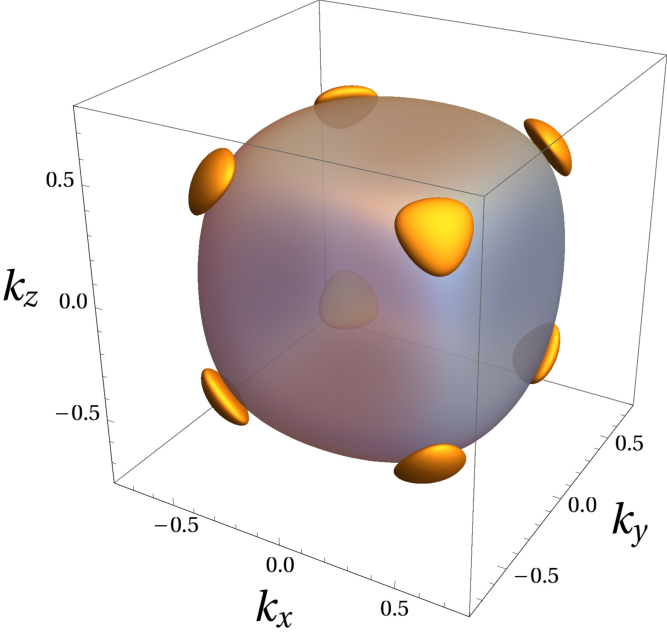
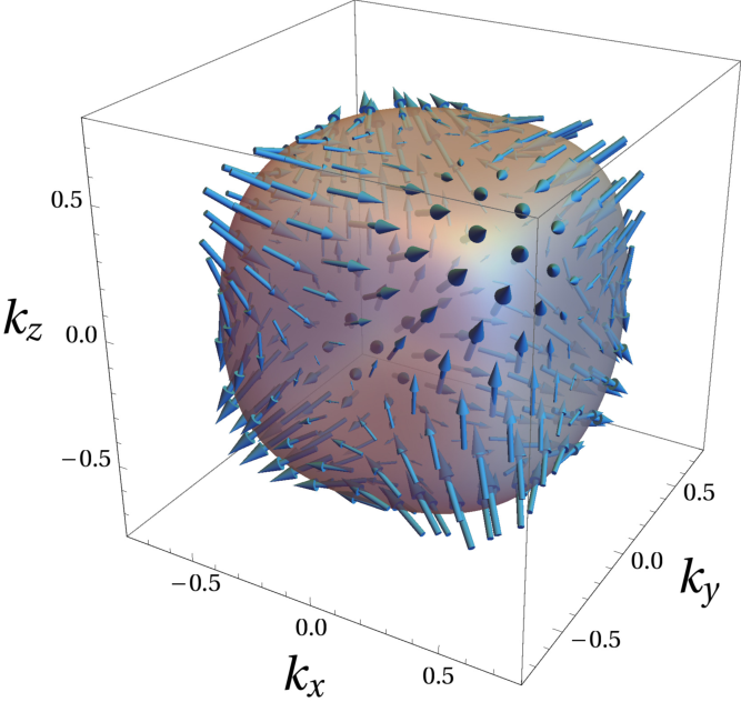
(a) (b) (c)

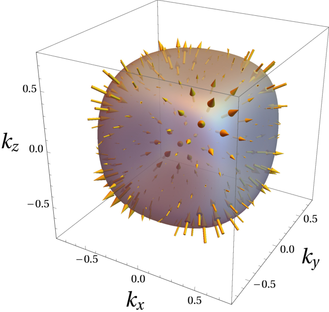
Figure 1: Low-energy structure of the TRSB $E_{g}$ pairing state with ${\bf h}=(1,i)$. (a) Bogoliubov Fermi surfaces (opaque orange) in comparison to the normal-state Fermi surface (semi-transparent). A gap amplitude of $\Delta_{0}=0.2\,\text{eV}$ has been used. (b) Pseudomagnetic field acting on the states at the Fermi surface due to the nonunitary pairing state. Note that the orientation is basis dependent and corresponds to our choice of the MCBB defined in Appendix A. (c) Magnetization of the states at the Fermi surface arising from the pseudomagnetic field.

III.1.1 $E_{g}$ pairing

For pairing restricted to states from the $E_{g}$ irrep, the general potential reads

$$\Delta=\Delta_{0}\,(h_{3z^{2}-r^{2}}\Gamma_{3z^{2}-r^{2}}+h_{x^{2}-y^{2}}\Gamma_{x^{2}-y^{2}})$$ (58)

so that the pairing state is characterized by the ordering vector $\mathbf{h}=(h_{3z^{2}-r^{2}},h_{x^{2}-y^{2}})$. A Landau analysis VoG85 ; SiU91 ; BWW16 gives $\mathbf{h}=(1,0)$, $(0,1)$, and $(1,i)$ as possible equilibrium solutions as well as symmetry-related vectors $\mathbf{h}$ obtained by applying point-group operations or time reversal. Since $\Gamma_{3z^{2}-r^{2}}$ and $\Gamma_{x^{2}-y^{2}}$ cannot be mapped into each other by any point-group symmetry, the pairing states $\mathbf{h}=(1,0)$ and $(0,1)$ do not generically have the same free energy VoG85 ; RGF17 ; SiU91 . The state with $\mathbf{h}=(1,i)$ breaks TRS. There are two symmetry partners, which are listed in table 1. As shown in Fig. 1(a), this state possesses Bogoliubov Fermi surfaces, replacing the eight point nodes expected along the $(111)$ and equivalent directions in the single-band case. The pockets and the whole quasiparticle band structure do not break any lattice symmetries. The only broken discrete symmetry is TRS.

The time-reversal-odd gap product for the TRSB $E_{g}$ state is given by

$$\Delta\Delta^{\dagger}-\Delta_{T}\Delta_{T}^{\dagger}=\frac{8}{\sqrt{3}}\,\Delta_{0}^{2}\left(J_{x}J_{y}J_{z}+J_{z}J_{y}J_{x}\right)\,.$$ (59)

This represents an octopolar magnetic order parameter and belongs to the irrep $A_{2g}$. It is interesting to note that this order parameter also appears in the context of frustrated magnetism on the pyrochlore lattice, where it describes all-in-all-out (AIAO) magnetic order of spins at the four corners of the elementary tetrahedra. The term appears in the single-particle mean-field Hamiltonian of the $j=3/2$ electron bands SMB14 ; GRDS17 ; BoH17 . The octopolar structure is clearly seen in the pseudomagnetic field in Fig. 1(b).

Although the pseudospin is not related in a simple way to the true spin, the pseudomagnetic field will generally be accompanied by a polarization of the physical spin since TRS is broken. We here define the magnetization as the expectation value of the total angular momentum $\mathbf{J}$. In the current theory, the magnetization contribution from states close to the normal-state Fermi surface at momentum $\mathbf{k}$ has the components

$$m_{\mathbf{k},\mu}=-\frac{1}{|\mathbf{v}_{\mathbf{k},-}|}\,\delta\mathbf{h}_{\mathbf{k},-}\cdot\operatorname{Tr\,}(\mathcal{P}_{\mathbf{k},-}\check{\mathbf{s}}\mathcal{P}_{\mathbf{k},-}J_{\mu})\,.$$ (60)

The derivation is relegated to Appendix B. Note that $m_{\mathbf{k},\mu}$ is independent of the specific choice of the pseudospin basis since both $\delta\mathbf{h}_{\mathbf{k},-}$ and $\check{\mathbf{s}}$ are transformed simultaneously when going from one basis to another. The magnetization is plotted in Fig. 1(c) and the octopolar structure is again readily apparent. The octopolar magnetic order implies that there is no overall magnetization in this state. Note that a pseudomagnetic field does not necessarily imply a magnetization at a given momentum: although $\delta{\bf h}_{{\bf k},-}$ is nonzero in the planes $k_{\mu}=0$, $\mu=x,y,z$, the magnetization vanishes in these directions.

III.1.2 $T_{2g}$ pairing

The general from of a pairing potential involving only states from the $T_{2g}$ irrep is

$$\Delta=\Delta_{0}\,(l_{yz}\Gamma_{yz}+l_{xz}\Gamma_{xz}+l_{xy}\Gamma_{xy})\,.$$ (61)

The pairing states in the $T_{2g}$ sector are characterized by different vectors $\mathbf{l}=(l_{yz},l_{xz},l_{xy})$. A Landau analysis VoG85 ; SiU91 ; BWW16 shows that the possible equilibrium solutions are $\mathbf{l}=(1,0,0)$, $(1,1,1)$, $(1,i,0)$, and ${\bf l}=(1,e^{2\pi i/3},e^{-2\pi i/3})$, as well as symmetry-related vectors $\mathbf{l}$. The two distinct TRSB pairing states correspond to $\mathbf{l}=(1,i,0)$ (chiral state) and ${\bf l}=(1,e^{2\pi i/3},e^{-2\pi i/3})$ (cyclic state). The symmetry partners of these states are listed in table 1. Since $\Gamma_{xz}$, $\Gamma_{yz}$, and $\Gamma_{xy}$ can be transformed into one another by rotations contained in $O_{h}$, these TRSB states are sixfold and eightfold degenerate, respectively.

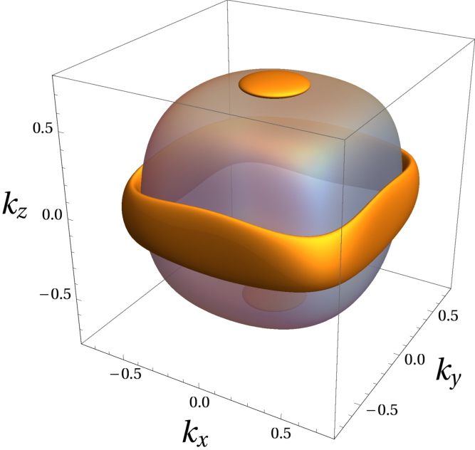
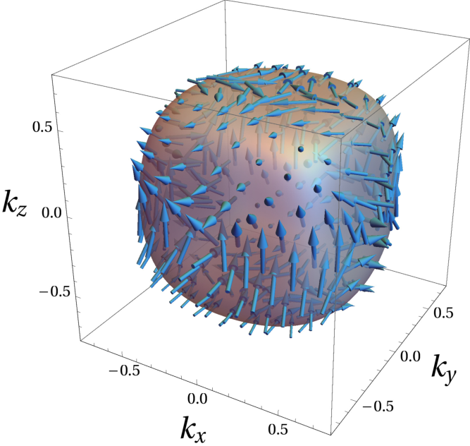
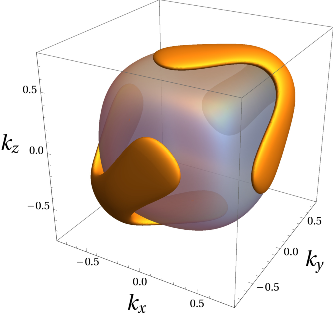
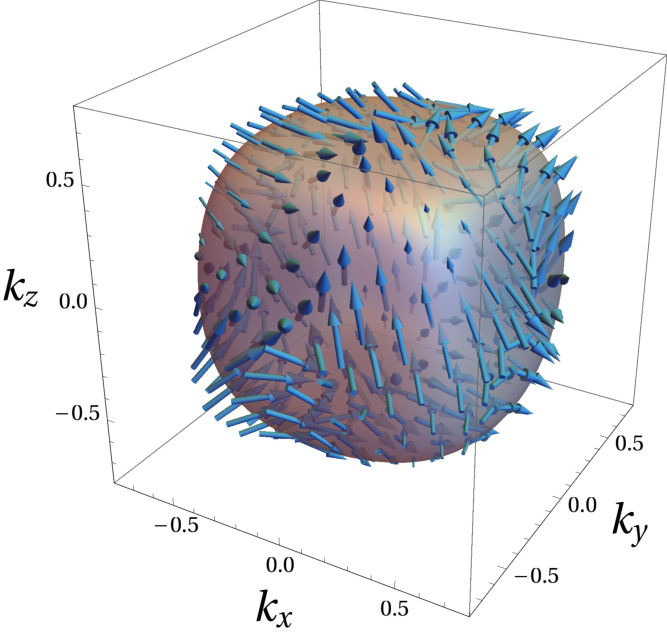
(a) (b) (c)
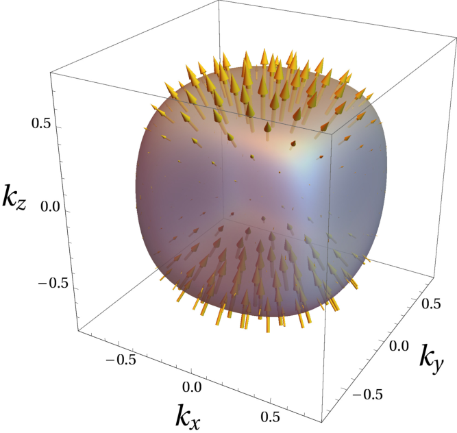
(d) (e) (f)

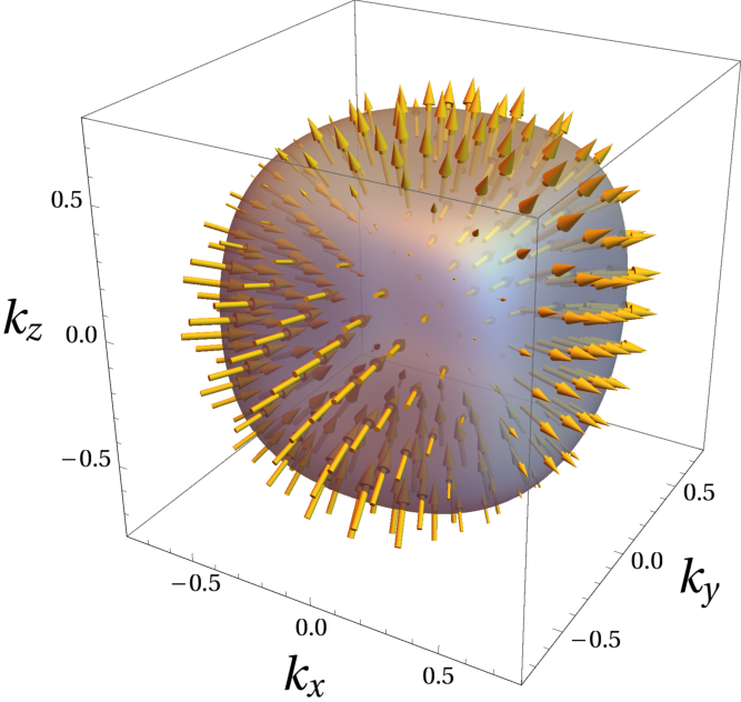
Figure 2: Low-energy structure of the TRSB $T_{2g}$ pairing states with ${\bf l}=(1,i,0)$ [(a)–(c)] and ${\bf l}=(1,e^{2\pi i/3},e^{-2\pi i/3})$ [(d)–(f)]. (a), (d) Bogoliubov Fermi surfaces (opaque orange) in comparison to the normal-state Fermi surface (semi-transparent). (b), (e) Pseudomagnetic field acting on the states at the Fermi surface. Note that the orientation is basis dependent and corresponds to our choice of the MCBB defined in Appendix A. (c), (f) Magnetization of the states at the Fermi surface arising from the pseudomagnetic field. For panels (a) and (d), a gap amplitude of $\Delta_{0}=0.2\,\mathrm{eV}$ has been used.

We first examine the chiral state, which was previously discussed in Ref. ABT17 . The line node in the $k_{x}k_{y}$ plane and the point nodes on the $k_{z}$ axis for the single-band model are inflated into toroidal and spheroidal pockets, respectively, as shown in Fig. 2(a). As evidenced by the Bogoliubov Fermi surfaces, the gap is nonunitary and the time-reversal-odd gap product is

$$\Delta\Delta^{\dagger}-\Delta_{T}\Delta_{T}^{\dagger}=\frac{4}{3}\,\Delta_{0}^{2}\left(7J_{z}-4J_{z}^{3}\right).$$ (62)

The gap product belongs to the irrep $T_{1g}$ (of which the spin operators $J_{\nu}$ are irreducible tensor operators), and involves both dipolar ($\propto J_{z}$) and octopolar ($\propto J_{z}^{3}$) contributions. Intriguingly, these appear in precisely the same combination as the order parameter of two-in-two-out order on the elementary tetrahedra of the pyrochlore lattice, which is associated with a polarization along the $z$-axis. The two-in-two-out condition constitutes the ice rule and leads to interesting spin-ice (SI) physics BoH17 ; GRDS17 .

The pseudomagnetic field of the low-energy states is shown in Fig. 2(b); although it displays a complicated vortex-like structure, an overall polarization in the $z$-direction is apparent, consistent with the dipole nature of the nonunitary part. The physical magnetization, presented in Fig. 2(c), clearly shows a net moment along the $z$-axis. Interestingly, the pseudomagnetic field in the vicinity of the toroidal Bogoliubov Fermi surface gives a negligible magnetization. The symmetry-related ${\bf l}=(0,1,i)$ and ${\bf l}=(i,0,1)$ states have a similar nodal (magnetic) structure, but with the point nodes (magnetization) oriented along the $x$- and $y$-axis, respectively.

In a single-band system, the cyclic state $\mathbf{l}=(1,\omega^{a},\omega^{b})$ with $\omega=e^{i\pi/3}$, see table 1, has point nodes along the three crystal axes, and two additional point nodes along the direction $(-1)^{a+b}\hat{\bf x}+(-1)^{b}\hat{\bf y}+(-1)^{a}\hat{\bf z}$, which remains a threefold rotational axis. However, instead of the expected eight Bogoliubov Fermi surfaces, Fig. 2(d) only shows two. This results from the merging of the Bogoliubov Fermi surfaces originating from the point nodes along the $[111]$ direction with the surfaces from the three nearest nodes along the crystal axes. Despite choosing the same gap magnitude in all figures, the merging of the Fermi surfaces is not seen in the $E_{g}$ or chiral $T_{2g}$ states for two reasons: First, the pairing state in the cyclic $T_{2g}$ state has three instead of two components, and hence the pseudomagnetic field has larger magnitude near the point nodes. Second, the would-be point nodes are relatively close together in momentum space and the superconducting gap between them remains significantly smaller than the gap far from the nodes. Choosing a smaller gap amplitude results in disconnected Bogoliubov Fermi surfaces: multiplying $\Delta_{0}$ by a factor of $1/4$ gives the nodal surfaces shown in Fig. 3. This is convenient, as we will later want to exhibit surface states between the projections of inflated nodes.

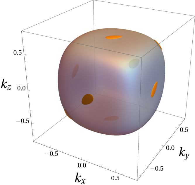
Figure 3: Small-gap form of the Bogoliubov Fermi surfaces (opaque orange) of the cyclic TRSB $T_{2g}$ pairing state with ${\bf l}=(1,e^{2\pi i/3},e^{-2\pi i/3})$ in comparison to the normal-state Fermi surface (semi-transparent). We have chosen the gap amplitude $\Delta_{0}=0.05\,\mathrm{eV}$ for this plot. For larger gap amplitudes, the eight Bogoliubov Fermi surfaces merge into two, as shown in Fig. 2(d).

The time-reversal-odd gap product for the cyclic state ${\bf l}=(1,\omega^{a},\omega^{b})$ reads

$$\Delta\Delta^{\dagger}-\Delta_{T}\Delta_{T}^{\dagger} =-\frac{4}{3}\,\Delta_{0}^{2}\,\bigg{(}\sin\frac{\pi\,(a-b)}{3}\,\hat{\bf x}+\sin\frac{\pi b}{3}\,\hat{\bf y}$$

$$\quad{}-\sin\frac{\pi a}{3}\,\hat{\bf z}\bigg{)}\cdot\left(7{\bf J}-4{\bf J}^{3}\right),$$ (63)

where ${\bf J}^{3}$ is the vector $(J_{x}^{3},J_{y}^{3},J_{z}^{3})$. Again, the nonunitary part has the same form as a magnetic order parameter on the pyrochlore lattice, in this case a spin-ice variant with magnetization along the threefold rotation axis. In Ref. GRDS17 , this is referred to as a three-in-one-out (3I1O) order. For the case of ${\bf l}=(1,\omega^{2},\omega^{-2})$, a net pseudomagnetic field along the threefold rotation axis is clearly visible in Fig. 2(e), in addition to a complicated field texture. Plotting the physical magnetization in Fig. 2(f), the existence of a net magnetic moment along the $[111]$ direction is evident.

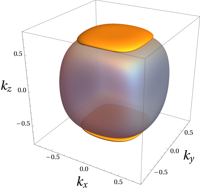
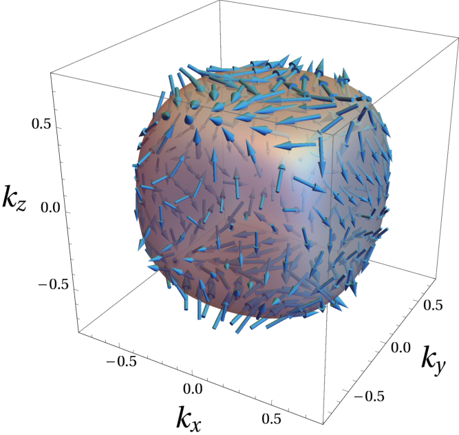
(a) (b) (c)

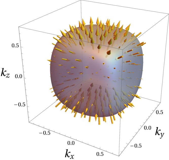
Figure 4: Low-energy structure of the TRSB mixed $E_{g}$-$T_{2g}$ pairing state of Eq. (64). (a) Bogoliubov Fermi surfaces (opaque orange) in comparison to the normal-state Fermi surface (semi-transparent). A gap amplitude of $\Delta_{0}=0.2\,\text{eV}$ has been used. (b) Pseudomagnetic field acting on the states at the Fermi surface due to the nonunitary pairing state. Note that the orientation is basis dependent and corresponds to our choice of the MCBB defined in Appendix A. (c) Magnetization of the states at the Fermi surface arising from the pseudomagnetic field.

III.1.3 Mixed pairing

The cases considered so far exhaust the essentially different TRSB pairing states that belong to a single irrep of $O_{h}$. As noted above, pairing amplitudes from different irreps may coexist if the corresponding pairing interactions are comparable RGF17 . An important example of such a state is provided by

$$\Delta=\Delta_{0}\,(\Gamma_{x^{2}-y^{2}}+i\Gamma_{xy})\,,$$ (64)

which mixes the $E_{g}$ and $T_{2g}$ irreps. Projected into the band states close to the zone center, this realizes a $(k_{x}+ik_{y})^{2}$-wave state. In contrast to the pure-irrep states for $O_{h}$, the single-band version supports point nodes with quadratic dispersion in the directions along the normal-state Fermi surface SiU91 ; RGF17 , so-called double Weyl points. Such nodal structures can appear for pure-irrep pairing in other points groups, e.g., for $D_{6h}$ as discussed below. The underlying point group is not essential for the topological properties of the states or the structure of the Bogoliubov Fermi surfaces, which are shown in Fig. 4(a). For the same value for the gap amplitude as in Figs. 1 and 2, we find much larger inflated nodes. The large nodal surfaces reflect the quadratic dispersion of the double Weyl points of the projected gap along the normal-state Fermi surface: since the dispersion is quadratic, a pseudomagnetic field of the same order as for the other cases leads to a much larger inflated node. The dimensions of the Bogoliubov Fermi surfaces can be estimated as follows ABT17 : In the direction perpendicular to the normal-state Fermi surface, the quasiparticle dispersion is proportional to $v_{F}\,\delta k_{\perp}$, where $\delta k_{\perp}$ is the distance from the Fermi surface. Since the pseudomagnetic field is proportional to $|\Delta_{0}|^{2}$, it follows that the size of the inflated nodes in the perpendicular direction scales as $\delta k_{\perp}\sim|\Delta_{0}|^{2}$. In the directions along the normal-state Fermi surface, the quasiparticle dispersion for a single-Weyl node (relevant for pure-irrep pairing) is proportional to $|\Delta_{0}|\,\delta k_{\|}$, where $\delta k_{\|}$ is the distance along the Fermi surface. Comparing this to the pseudomagnetic field proportional to $|\Delta_{0}|^{2}$, we find that the size of the inflated nodes along the normal-state Fermi surface scales as $\delta k_{\|}\sim|\Delta_{0}|$. In the present case of a quadratic point node, however, the energy in the parallel direction is proportional to $|\Delta_{0}|\,(\delta k_{\|})^{2}$ so that the size of the inflated nodes scales as $\delta k_{\|}\sim|\Delta_{0}|^{1/2}$.

The mixed-irrep state is nonunitary and has the time-reversal-odd gap product

$$\Delta\Delta^{\dagger}-\Delta_{T}\Delta_{T}^{\dagger}=\frac{2}{3}\,\Delta_{0}^{2}\left(13J_{z}-4J_{z}^{3}\right).$$ (65)

This belongs to the $T_{1g}$ irrep and resembles the nonunitary part for the chiral $T_{2g}$ state. In contrast to the nonunitary part of the pure-irrep TRSB state, Eq. (65) does not have a straightforward interpretation in terms of magnetically ordered states of the pyrochlore lattice. The pseudomagnetic field associated with the mixed-irrep pairing state is shown in Fig. 4(b). It displays pronounced vortex-like structures similar to those of the chiral $T_{2g}$ state. The physical magnetization presented in Fig. 4(c) evidences a net moment along the $z$-axis.

(a)

(b)

Figure 5: Dispersion of the surface bands in the normal state for (a) the $(111)$ surface and (b) the $(100)$ surface, for a thickness of $W=1000$. The projection of the bulk Fermi sea is shown in gray.

III.2 Surface states

Surface states are studied by diagonalizing the BdG Hamiltonian Eq. (2) implemented on a real-space slab of finite thickness. We will consider $(111)$ and $(100)$ surfaces, as well as their symmetry partners. The slabs preserve translation symmetry in two directions so that the Hamiltonian can be block diagonalized by Fourier transformation in these directions. Each block has the dimension $8W\times 8W$, where $W$ is the number of layers in the slab. The wave vector parallel to the surfaces is written as $\mathbf{k}_{\|}=k_{1}\,(1,-1,0)^{T}/\sqrt{2}+k_{2}\,(1,1,-2)^{T}/\sqrt{6}$ for the $(111)$ case and as $\mathbf{k}_{\|}=k_{1}\,(0,1,1)^{T}/\sqrt{2}+k_{2}\,(0,-1,1)^{T}/\sqrt{2}$ for the $(100)$ case. More details can be found in Ref. TSA17 .

In the following, we study the surface states of the TRSB states with Bogoliubov Fermi surfaces introduced above. The model system possesses surface states even in the normal phase DyaK81 , which form bands that emanate from the quadratic band-touching point. They are analogous to the surface bands in noncentrosymmetric half-Heusler materials CSL11 ; LYW16 ; TSA17 , except that they are twofold spin degenerate due to the IS in point group $O_{h}$. For later comparison with the superconducting states, the dispersion of the surface band closest to the Fermi energy is shown in Fig. 5 for the $(111)$ and $(100)$ surfaces. The plots would of course be identical for directions related by point-group symmetries; this will not be the case for some of the superconducting states since these break lattice symmetries. Note that the $k_{1}$ and $k_{2}$ axes for the $(100)$ surface are rotated by $45^{\circ}$ relative to the cubic $k_{y}$ and $k_{z}$ axes.

The surface bands in Fig. 5 cross the Fermi energy, seen as smooth changes from blue through black to red, i.e., there are one-dimensional Fermi lines of surface states. These Fermi lines are not protected; the surface bands can be continuously deformed so that they do not cross the Fermi energy. Their presence is nevertheless interesting since it allows us to study their fate when superconductivity sets in.

Figure 6: Dispersion of the surface bands in the $E_{g}$ pairing state with $\mathbf{h}=(1,i)$ for the $(111)$ surface. The thickness is $W=1000$. Only a close-up of the region of the normal-state Fermi sea is shown. The spectrum at each momentum is symmetric, the color refers to the absolute value of the corresponding two energies $\pm\epsilon(k_{1},k_{2})$. The projections of the Bogoliubov Fermi pockets are shown in gray. In the white regions, no surface states are found.

We first consider the $E_{g}$ state with $\mathbf{h}=(1,i)$. The surface dispersion for the $(111)$ surface is shown in Fig. 6, which should be compared to Fig. 5(a) for the normal state. We clearly see the projections of the eight equivalent spheroidal Fermi pockets, where the two in the $[111]$ and $[\bar{1}\bar{1}\bar{1}]$ directions are projected on top of each other. In addition, there are arcs of zero-energy surface states connecting the other six projected pockets. Since the spectrum at each $(k_{1},k_{2})$ consists of pairs $\pm\epsilon(k_{1},k_{2})$, two dispersive surface bands with opposite velocities cross at each arc. An analysis of the corresponding states shows that the two bands consist of states localized at opposite surfaces. Hence, there are two arcs originating from each of the outer pockets at each surface. The associated velocities are found to point in the same direction for the two arcs at the same surface, i.e., they have the same chirality. The two arcs per surface are in agreement with the pockets having Chern numbers $\pm 2$, see Sec. V.1 below. For the central two pockets, no arcs are present, consistent with their Chern numbers adding up to zero.

(a)

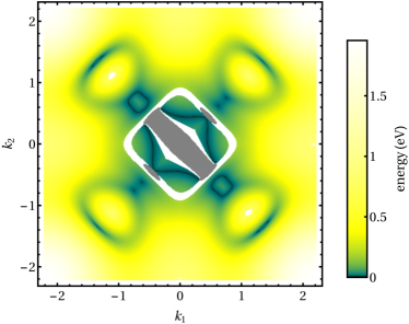
(b)

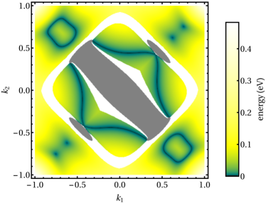
Figure 7: (a) Dispersion of the surface bands in the chiral $T_{2g}$ pairing state with $\mathbf{l}=(1,i,0)$ for the $(100)$ surface. The thickness is $W=1000$. (b) Close-up of the central region of panel (a), where in the normal state the Fermi sea would be found. The spectrum at each momentum is symmetric, the color refers to the absolute value of the corresponding two energies $\pm\epsilon(k_{1},k_{2})$. The projections of the Bogoliubov Fermi pockets are shown in gray. In the white regions, no surface states are found.

Next, we turn to the chiral $T_{2g}$ pairing state with $\mathbf{l}=(1,i,0)$. The chosen gap amplitude is the same as for the $E_{g}$ state. Figure 7 shows the surface dispersion for the $(100)$ surface. The plot should be compared to Fig. 5 (b) for the normal state. The surface bands originating from the normal state survive but their Fermi lines are mostly gapped out and replaced by valleys at nonzero energy. Instead, the surface bands develop new nodal lines, which are seen as closed, black loops in Fig. 7. These lines are not topologically protected and hence their existence and shape depends on details of the model. The projections of the two spheroidal and the toroidal Fermi pockets, see Fig. 2(a), are also clearly visible in Fig. 7. In addition, each projected spheroidal pocket is connected to the projected toroidal pocket by two Fermi arcs, in agreement with Chern numbers of $\pm 2$ for the spheroidal pockets. The two arcs localized at the same surface have the same chirality, as expected. The arcs can also be understood in terms of twofold degenerate arcs as found by Tamura et al. TKB17 for a single-band model, which are split into two by the pseudomagnetic field ABT17 . As we will see, the toroidal pocket has Chern number $0$ and thus does not impose the presence of any arcs. However, its large projection is in the way of the arcs from the spheroidal pockets. There are four arcs connected to the projection of the toroidal pocket, with their chirality summing to zero.

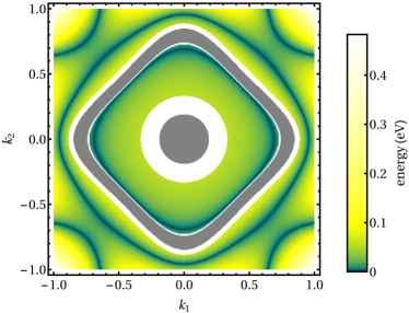
Figure 8: Dispersion of the surface bands in the chiral $T_{2g}$ pairing state with $\mathbf{l}=(1,i,0)$ as in Fig. 7(b), but for the $(001)$ surface.

Figure 7 shows the projection of the inflated line node on edge. Since line nodes in other topological superconductors, namely noncentrosymmetric ones that preserve TRS, are accompanied by flat surface bands TMY10 ; STY11 ; BST11 ; ScR11 ; SBT12 ; ScB15 , one might ask whether the same is true here. To check this, we plot in Fig. 8 the surface dispersion for the $(001)$ surface. The projection of the inflated line node is clearly visible as the rounded gray square. Obviously, there is no flat band delimited by the projected node. Indeed, a flat band is not expected since the inflated line node is protected by nontrivial Pfaffians in each mirror-parity sector, as discussed further in Sec. V.2. These Pfaffians are only defined in the mirror-invariant $k_{z}=0$ plane. The nature of line nodes in noncentrosymmetric superconductors with TRS is different: they are protected by winding numbers calculated along closed loops around the node. The argument for the existence of flat bands relies on the deformation of these loops into straight lines perpendicular to the surface SBT12 ; ScB15 . Such a construction is not possible for the present case of nodes protected by a mirror symmetry.

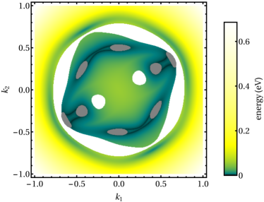
Figure 9: Dispersion of the surface bands in the cyclic $T_{2g}$ pairing state with $\mathbf{l}=(1,e^{2\pi i/3},e^{-2\pi i/3})$ for the ($1\bar{1}1$) surface. The thickness is $W=1000$. Only a close-up of the region of the normal-state Fermi sea is shown. The spectrum at each momentum is symmetric, the color refers to the absolute value of the corresponding two energies $\pm\epsilon(k_{1},k_{2})$. The projections of the Bogoliubov Fermi pockets are shown in gray. In the white regions, no surface states are found.

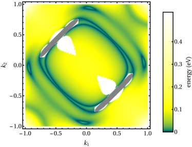
Figure 10: Dispersion of the surface bands in the mixed $E_{g}$-$T_{2g}$ pairing state for the $(100)$ surface. The thickness is $W=1000$. Only a close-up of the region of the normal-state Fermi sea is shown. The spectrum at each momentum is symmetric, the color refers to the absolute value of the corresponding two energies $\pm\epsilon(k_{1},k_{2})$. The projections of the Bogoliubov Fermi pockets are shown in gray. In the white regions, no surface states are found.

The cyclic $T_{2g}$ pairing state with $\mathbf{l}=(1,e^{2\pi i/3},e^{-2\pi i/3})$ only has inflated point nodes. We consider the ($1\bar{1}1$) surface here. This is equivalent to the $(111)$ surface for $\mathbf{l}=(1,e^{\pi i/3},e^{-\pi i/3})$. The $(111)$ surface for $\mathbf{l}=(1,e^{2\pi i/3},e^{-2\pi i/3})$ is less instructive since two of the Fermi pockets are projected on top of each other. The dispersion of surface states is shown in Fig. 9 for the smaller gap amplitude $\Delta_{0}=0.05\,\mathrm{eV}$, for which the Bogoliubov Fermi pockets are separated. The Fermi pockets are shown in Fig. 3 above. The projections of the eight Fermi pockets are clearly visible in Fig. 9. Note that the two at the larger distance from the center are inequivalent to the other six. All pockets are connected by Fermi arcs in pairs. There are two arcs associated with each pocket, as expected for Chern numbers of $\pm 2$.

Finally, we consider the mixed-irrep pairing state of Eq. (64). The surface dispersion for the $(100)$ surface is shown in Fig. 10. The edge-on projections of the large Bogoliubov Fermi pockets are clearly visible. Four arcs emanate from each of them, unlike for the inflated point nodes encountered so far. It is natural to attribute the doubled number of arcs to the double-Weyl nature of the original point nodes. Four arcs would be consistent with Chern numbers $\mathrm{Ch}_{1}=\pm 4$. We will see in Sec. V.1 that this is indeed the correct explanation.

IV Hexagonal superconductors

In the context of unconventional superconductivity, the $j=3/2$ description of the $\Gamma_{8}$ bands in a cubic system is rather unfamiliar. Pairing of four-component fermions is more commonly encounted when the low-energy electron states have well-defined orbital and spin degrees of freedom, as in Sr₂RuO₄ or the iron-pnictide superconductors. To show how our analysis works for such a case, we consider the example of a hypothetical hexagonal superconductor with point group $D_{6h}$, where the low-energy electron states arise from orbitals belonging to the two-dimensional irrep $E_{1g}$. Selecting orbitals from a two-dimensional irrep ensures that both orbitals will have equal weight at the Fermi surface, and therefore represents a more generic origin of the four-component fermions as compared to the accidental near-degeneracy of two orbitals from different irreps. Choosing orbitals which belong to one of the three other two-dimensional irreps does not introduce qualitatively new physics.

The normal-state block of the BdG Hamiltonian Eq. (2) reads

$$H_{0}(\mathbf{k}) =\bigg{[}\epsilon_{00}-(t_{xy}+t_{xyz}\cos k_{z})\bigg{(}\cos k_{x}+2\cos\frac{k_{x}}{2}\cos\frac{\sqrt{3}k_{y}}{2}\bigg{)}-t_{z}\cos k_{z}-\mu\bigg{]}\chi_{0}\otimes\sigma_{0}$$

$$\quad{}+\bigg{[}\epsilon_{23}-(t^{\prime}_{xy}+t^{\prime}_{xyz}\cos k_{z})\bigg{(}\cos k_{x}+2\cos\frac{k_{x}}{2}\cos\frac{\sqrt{3}k_{y}}{2}\bigg{)}-t^{\prime}_{z}\cos k_{z}\bigg{]}\chi_{2}\otimes\sigma_{3}$$

$$\quad{}-(t^{\text{inter}}_{xy}+t^{\text{inter}}_{xyz}\cos k_{z})\bigg{[}\bigg{(}\cos k_{x}-\cos\frac{k_{x}}{2}\cos\frac{\sqrt{3}k_{y}}{2}\bigg{)}\chi_{3}\otimes\sigma_{0}-\sqrt{3}\sin\frac{k_{x}}{2}\sin\frac{\sqrt{3}k_{y}}{2}\chi_{1}\otimes\sigma_{0}\bigg{]}$$

$$\quad{}-2\,t_{\text{soc}}\sin k_{z}\bigg{[}\bigg{(}2\cos\frac{k_{x}}{2}+\cos\frac{\sqrt{3}k_{y}}{2}\bigg{)}\sin\frac{k_{x}}{2}\,\chi_{2}\otimes\sigma_{1}+\sqrt{3}\cos\frac{k_{x}}{2}\sin\frac{\sqrt{3}k_{y}}{2}\,\chi_{2}\otimes\sigma_{2}\bigg{]}\,,$$ (66)

where $\sigma_{\mu}$ and $\chi_{\mu}$ are Pauli matrices describing the spin and the orbital degree of freedom, respectively. This tight-binding model includes nearest-neighbor hopping in the xy plane and normal to the plane and also next-nearest-neighbor hopping out of plane. We note that the third line describes orbitally nontrivial hopping, while the second and fourth lines describe spin-orbit coupling. Their matrix structure is determined by the transformation properties of the orbitals under point-group operations. The momentum-dependent prefactors are constrained by the periodicity in reciprocal space and by $H_{0}(\mathbf{k})$ having to transform trivially, i.e., according to the irrep $A_{1g}$.

The fundamental difference of the normal-state band structure of the hexagonal model compared to the cubic case is that there is no symmetry-protected band-touching point at $\mathbf{k}=0$ since the double group $D_{6h}$ does not have any four-dimensional irreps DDJ08 . The five nontrivial Kronecker products appearing in Eq. (66) are a representation of the Euclidean Dirac matrices. We can set

$$\gamma^{1} =\chi_{2}\otimes\sigma_{3}\,,$$ (67)

$$\gamma^{2} =\chi_{2}\otimes\sigma_{1}\,,$$ (68)

$$\gamma^{3} =\chi_{2}\otimes\sigma_{2}\,,$$ (69)

$$\gamma^{4} =\chi_{1}\otimes\sigma_{0}\,,$$ (70)

$$\gamma^{5} =\chi_{3}\otimes\sigma_{0}$$ (71)

so that the unitary part of the time-reversal operator is

$$U_{T}=\gamma^{1}\gamma^{2}=\chi_{0}\otimes i\sigma_{2}\,.$$ (72)

The orbital degree of freedom is therefore invariant under time reversal. For the numerical calculations we take $\epsilon_{00}=6.625\,\mathrm{eV}$, $\epsilon_{23}=5.3\,\mathrm{eV}$, $t_{z}=1.5\,\mathrm{eV}$, $t_{xy}=0.667\,\mathrm{eV}$, $t_{xyz}=-0.333\,\mathrm{eV}$, $t_{z}^{\prime}=2\,\mathrm{eV}$, $t_{xy}^{\prime}=0.8\,\mathrm{eV}$, $t_{xyz}^{\prime}=0.133\,\mathrm{eV}$, $t_{xy}^{\text{inter}}=0.462\,\mathrm{eV}$, $t_{xyz}^{\text{inter}}=-0.231\,\mathrm{eV}$, $t_{\text{soc}}=-0.231\,\mathrm{eV}$, and $\mu=3.300\,\mathrm{eV}$, yielding an ellipsoidal Fermi surface for the $-$ states at the zone center.

The local pairing is described in terms of the six matrices

$$A_{1g}\mbox{:} \Gamma_{s} =U_{T}\,,\phantom{abcdefghijklm}$$ (73)

$$\Gamma_{s^{\prime}} =(\chi_{2}\otimes\sigma_{3})\,U_{T}\,,$$ (74)

$$E_{1g}\mbox{:} \Gamma_{xz} =(\chi_{2}\otimes\sigma_{1})\,U_{T}\,,$$ (75)

$$\Gamma_{yz} =(\chi_{2}\otimes\sigma_{2})\,U_{T}\,,$$ (76)

$$E_{2g}\mbox{:} \Gamma_{x^{2}-y^{2}} =(\chi_{3}\otimes\sigma_{0})\,U_{T}\,,$$ (77)

$$\Gamma_{xy} =(\chi_{1}\otimes\sigma_{0})\,U_{T}\,.$$ (78)

The labeling of the matrices reflects the form of the gap when projected onto the states near the zone center: the $A_{1g}$ states are $s$-wave-like, whereas the $E_{1g}$ and the $E_{2g}$ states resemble $(k_{x}k_{z},k_{y}k_{z})$-waves and $(k_{x}^{2}-k_{y}^{2},k_{x}k_{y})$-waves, respectively. The unconventional $A_{1g}$ state and the $E_{1g}$ states represent orbital-singlet spin-triplet pairing, whereas the $E_{2g}$ states involve orbital-triplet spin-singlet pairing.

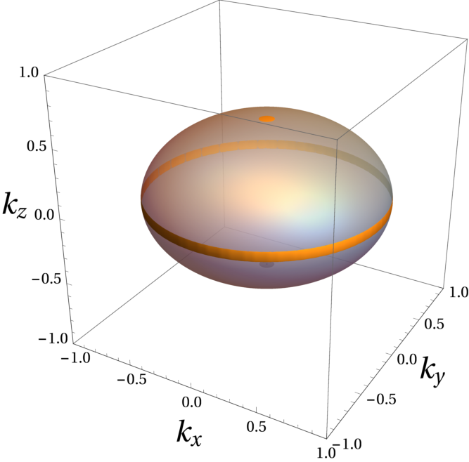
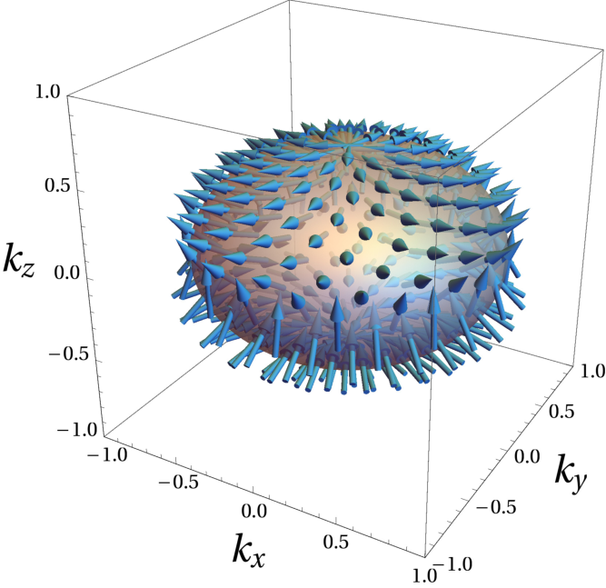
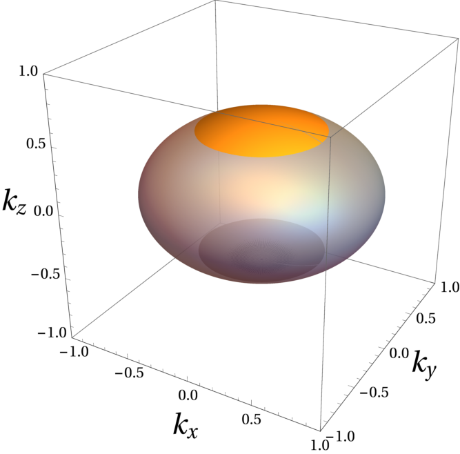
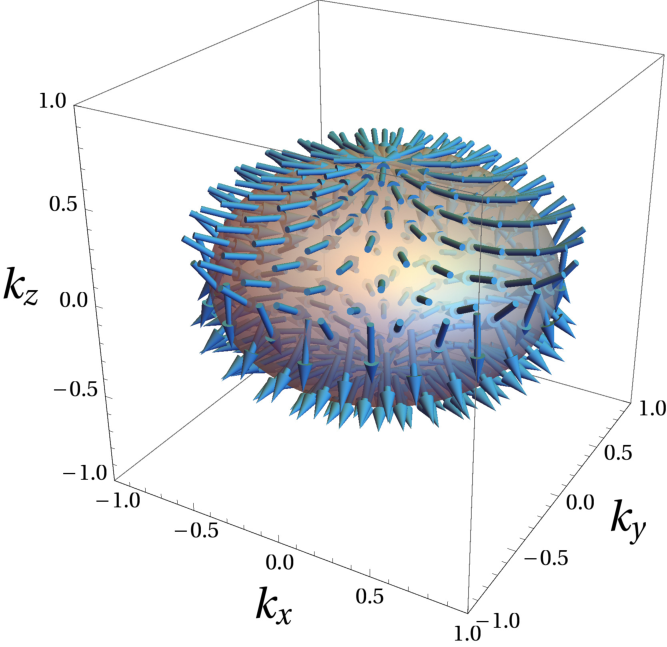
(a) (b) (c)
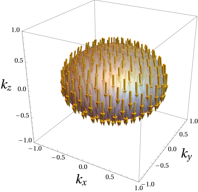
(d) (e) (f)

Figure 11: Low-energy structure of the TRSB $E_{1g}$ [(a)–(c)] and $E_{2g}$ [(d)–(f)] pairing states. (a), (d) Bogoliubov Fermi surfaces (opaque orange) in comparison to the normal-state Fermi surface (semi-transparent). (b), (e) Pseudomagnetic field acting on the states at the Fermi surface. Note that the orientation is basis dependent and corresponds to our choice of the MCBB defined in Appendix A. (c), (f) Magnetization of the states at the Fermi surface arising from the pseudomagnetic field. For panels (a) and (d), a gap amplitude of $\Delta_{0}=0.02\,\mathrm{eV}$ has been used.

IV.1 TRSB pairing

Restricting ourselves to pure-irrep pairing, two TRSB pairing states are allowed in our model:

$$\Delta_{E_{1g}} =\Delta_{0}\,(\Gamma_{xz}+i\Gamma_{yz})\,,$$ (79)

$$\Delta_{E_{2g}} =\Delta_{0}\,(\Gamma_{x^{2}-y^{2}}+i\Gamma_{xy})\,.$$ (80)

The single-band analogue of the $E_{1g}$ state is a $k_{z}(k_{x}+ik_{y})$-wave state SiU91 ; VoG85 , similar to the chiral $T_{2g}$ state of the cubic superconductor. It is thus expected to have line nodes in the $k_{z}=0$ plane and point nodes on the $k_{z}$ axis. In the single-band limit, the nodal structure of the $E_{2g}$ pairing resembles the $(k_{x}+ik_{y})^{2}$-wave state SiU91 ; VoG85 , with double Weyl points on the $k_{z}$-axis. In the two-band system considered here, these nodes are inflated into Bogoliubov Fermi surfaces, which are shown in Figs. 11(a) and (d). The Fermi surfaces are similar to the corresponding chiral $T_{2g}$ and mixed-irrep states, respectively, for the $O_{h}$ point group. Since for the $E_{2g}$ state the single-band variant has a double Weyl point, the mechanism explained in Sec. III.1.3 leads to large inflated nodes in the multiband case. For this reason, a small gap amplitude has been chosen for Fig. 11.

An interesting distinction between the two states is provided by the time-reversal-odd gap product:

$$\Delta_{E_{1g}}^{\phantom{\dagger}}\Delta_{E_{1g}}^{\dagger}-\Delta_{T,E_{1g}}^{\phantom{\dagger}}\Delta_{T,E_{1g}}^{\dagger} =4\Delta_{0}^{2}\,\chi_{0}\otimes\sigma_{3}\,,$$ (81)

$$\Delta_{E_{2g}}^{\phantom{\dagger}}\Delta_{E_{2g}}^{\dagger}-\Delta_{T,E_{2g}}^{\phantom{\dagger}}\Delta_{T,E_{2g}}^{\dagger} =4\Delta_{0}^{2}\,\chi_{2}\otimes\sigma_{0}\,.$$ (82)

Although in both cases this product belongs to the irrep $A_{2g}$, for the $E_{1g}$ case it represents a purely magnetic order, whereas in the $E_{2g}$ case it corresponds to chiral orbital order. This reflects the spin- and orbital-triplet nature of these pairing states, respectively.

The pseudomagnetic field is shown in Fig. 11(b) and (e). Remarkably, the two states have almost identical $\delta{\bf h}_{{\bf k},-}$, albeit with opposite sign, although their nodal structure and spin-orbital character are quite different. From this, we obtain the physical magnetization in analogy to the cubic case,

$$m_{\mathbf{k},\mu}=-\frac{1}{|\mathbf{v}_{\mathbf{k},-}|}\,\delta\mathbf{h}_{\mathbf{k},-}\cdot\operatorname{Tr\,}\mathcal{P}_{\mathbf{k},-}\check{\mathbf{s}}\mathcal{P}_{\mathbf{k},-}\chi_{0}\otimes\sigma_{\mu}\,.$$ (83)

As expected from the pseudomagnetic field, the physical magnetization is also very similar: in both cases an almost uniform magnetization across the Fermi surface is observed with net moment along the $z$-axis, but with opposite sign. Although such a polarization is not surprising for the $E_{1g}$ state in view of the explicitly magnetic form of the time-reversal-odd gap product, it is less obvious for the $E_{2g}$ state, for which the time-reversal-odd gap product corresponds to orbital order. The origin of the magnetization in the latter case is the strong spin-orbit coupling, in particular the term in the second line of Eq. (66), which converts the orbital polarization into a spin polarization.

(a)

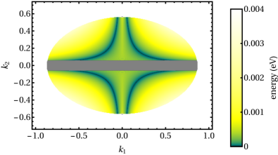
(b)

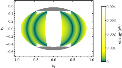
Figure 12: Dispersion of the surface bands at the $(010)$ surface for the TRSB (a) $E_{1g}$ and (b) $E_{2g}$ states. The thickness of the slab is $W=3000$. Only a close-up of the region of the normal-state Fermi sea is shown. The spectrum at each momentum is symmetric, the color refers to the absolute value of the corresponding two energies $\pm\epsilon(k_{1},k_{2})$. The projections of the Bogoliubov Fermi pockets are shown in gray. In the white regions, no surface states are found. The white region in the center of panel (b) is probably an artifact of the finite thickness.

IV.2 Surface states

We next consider the surface states at the $(010)$ surface, i.e., the one normal to the $k_{y}$-axis. We do not find surface bands in the normal state. This is expected since the normal-state surface bands for the cubic model originate from the topologically nontrivial band-touching point at $\mathbf{k}=0$, which does not exist for the $D_{6h}$ point group. Figure 12 shows the surface dispersion for the $E_{1g}$ and $E_{2g}$ pairing states. Surface bands only appear where the normal-state Fermi sea has been gapped out, which is consistent with the absence of surface bands in the normal state. For $E_{1g}$ pairing, two Fermi arcs emanate from each of the two spheroidal Fermi pockets, consistent with Chern number $\mathrm{Ch}_{1}=\pm 2$. Note that the Fermi pockets are so thin that they are essentially invisible if viewed from the edge. For the $E_{2g}$ case, we find that the localization length of surface states becomes very large for $k_{1}$ approaching zero so that for small $k_{1}$ they become indistinguishable from bulk states even for the large thickness of $W=3000$ used here. The white region in the center of Fig. 12 (b) is thus expected to be at least partially an artifact of the finite thickness. There are four arcs emanating from each inflated node, consistent with the Chern numbers $\mathrm{Ch}_{1}=\pm 4$.

V Topological invariants

The Bogoliubov Fermi pockets are protected by a $\mathbb{Z}_{2}$ invariant, which we have identified as the relative sign of the Pfaffian of the unitarily transformed BdG Hamiltonian on the two sides of the Fermi surface ABT17 . For a single band, pairing states with the same symmetries as the ones discussed above have point and line nodes that are protected by topological invariants. Specifically, the point nodes have nonzero Chern numbers, while the line node for the chiral $T_{2g}$ state with $\mathbf{l}=(1,i,0)$ is protected by a mirror symmetry ChS14 ; CTS16 ; BWR16 ; BzS17 . It is natural to ask whether these invariants survive in the multiband case, where the nodes are inflated into Bogoliubov Fermi surfaces. In the following, we illustrate our general considerations using the example provided by the $j=3/2$ pairing states of the cubic superconductor discussed above.

V.1 Chern invariant

For $CP$ symmetry satisfying $(CP)^{2}=+1$, point nodes have a $2\mathbb{Z}$ invariant, which is given by the first Chern number for a closed surface $\mathcal{S}$ surrounding the node ZSW16 . This Chern number is given by XCN10 ; She12 ; CTS16 ; BzS17

$$\mathrm{Ch}_{1}=\frac{1}{2\pi}\sum_{n\>\mathrm{occ.}}\oint_{\mathcal{S}}d^{2}\mathbf{s}(\mathbf{k})\cdot\big{[}\nabla_{\mathbf{k}}\times\mathbf{A}_{n}(\mathbf{k})\big{]}\,,$$ (84)

where $d^{2}\mathbf{s}(\mathbf{k})$ is a vectorial surface element in momentum space and $\mathbf{A}_{n}(\mathbf{k})$ is the Berry connection for the n-th band,

$$\mathbf{A}_{n}(\mathbf{k})=i\,\langle u_{n}(\mathbf{k})|\nabla_{\mathbf{k}}|u_{n}(\mathbf{k})\rangle\,,$$ (85)

in terms of the Bloch states $|u_{n}(\mathbf{k})\rangle$. The sum in Eq. (84) is over the occupied bands. Note that Eq. (84) only holds if the occupied bands are nondegenerate on $\mathcal{S}$ CTS16 , which is the case here since TRS is broken. It is worth emphasizing that this is not a classification of nodal points but rather of closed surfaces $\mathcal{S}$ in momentum space for which the gap does not close anywhere on $\mathcal{S}$. A nonzero Chern number guarantees that the gap closes somewhere in the enclosed volume but this need not happen at a single point.

Following Berry Ber84 , one can rewrite the Chern number as a Kubo-type expression,

$$\mathrm{Ch}_{1} =\frac{i}{2\pi}\sum_{n\>\mathrm{occ.}}\sum_{m\neq n}\oint_{\mathcal{S}}d^{2}\mathbf{s}(\mathbf{k})$$

$${}\cdot\frac{\langle u_{n}(\mathbf{k})|(\nabla_{\mathbf{k}}\mathcal{H})|u_{m}(\mathbf{k})\rangle\times\langle u_{m}(\mathbf{k})|(\nabla_{\mathbf{k}}\mathcal{H})|u_{n}(\mathbf{k})\rangle}{(E_{\mathbf{k}n}-E_{\mathbf{k}m})^{2}}\,,$$ (86)

where $E_{\mathbf{k}n}$ is the eigenenergy of the Bloch state $|u_{n}(\mathbf{k})\rangle$. This form is useful for the numerical evaluation since it is independent of the choice of phases of the Bloch states. With this, the eight spheroidal Fermi pockets for the $E_{g}$ state with $\mathbf{h}=(1,i)$, shown in Fig. 1(a), have $\mathrm{Ch}_{1}=\pm 2$. The sign of $\mathrm{Ch}_{1}$ for neighboring pockets is opposite.

The surfaces enclosing the upper (lower) spheroidal Fermi pocket for the chiral $T_{2g}$ state, shown in Fig. 2(a), are found to have Chern number $\mathrm{Ch}_{1}=-2$ ($+2$). Surfaces enclosing the whole toroidal pocket have $\mathrm{Ch}_{1}=0$. For the cyclic $T_{2g}$ state, shown in Fig. 3, there are two distinct classes of inflated point nodes. Their Chern numbers of $\mathrm{Ch}_{1}=\pm 2$ are indicated in Fig. 13. The Chern numbers of the three pockets on the cubic axes and next to one of the pockets at a corner are equal to each other but opposite to the one of the pocket at the corner. Hence, the Chern numbers of the four Bogoliubov Fermi pockets that merge for larger pairing amplitudes add up to $\pm 4$, which are thus the values for the large pockets of complicated shape shown in Fig. 2(d).

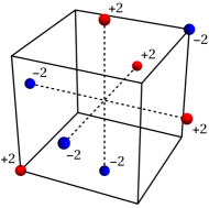
Figure 13: Schematic of the locations and Chern numbers of the inflated point nodes for the cyclic $T_{2g}$ pairing state with $\mathbf{l}=(1,e^{2\pi i/3},e^{-2\pi i/3})$ and sufficiently small pairing amplitude. Compare Fig. 3.

Finally, in the mixed-irrep $\Gamma_{x^{2}-y^{2}}+i\Gamma_{xy}$ state, the large upper (lower) pocket seen in Fig. 4(a) has Chern number $\mathrm{Ch}_{1}=+4$ ($-4$). Our results for the Chern numbers of the inflated point nodes are consistent with the Berry curvature obtained in RGF17 .

In summary, the spheroidal pockets for all considered pairing states are protected by Chern invariants, in agreement with a recent analysis by Bzdušek and Sigrist BzS17 . Consequently, the pockets can shrink to points but not vanish unless they annihilate pairwise. There is no corresponding protection of the toroidal pocket for the chiral $T_{2g}$ state. The Chern numbers are all even, as expected for $CP$-symmetric superconductors ZSW16 . They are also consistent with the observed number of Fermi arcs of surface states, namely two for pockets with $\mathrm{Ch}_{1}=\pm 2$ and four in the case of $\mathrm{Ch}_{1}=\pm 4$.

We thus find that the inflated point nodes (spheroidal pockets) are protected by two distinct invariants: an even Chern number and a Pfaffian KST14 ; ZSW16 ; ABT17 . Bzdušek and Sigrist BzS17 have recently formulated a comprehensive theory of nodal points, lines, and surfaces protected by two invariants, which they have dubbed “multiply charged nodes.”

V.2 Additional Pfaffians

Neither the Altland-Zirnbauer class D nor $CP$ symmetry squaring to $+1$ leads to invariants protecting line nodes in three dimensions ZSW16 . Hence, lattice symmetries are required for constructing an invariant for the line node in the single-band version of the chiral $T_{2g}$ state. In the following, we show that this also holds for the toroidal Fermi pocket in the multiband case.

The BdG Hamiltonian satisfies mirror symmetry in the $xy$ plane:

$$U_{\sigma z}\,\mathcal{H}(k_{x},k_{y},-k_{z})\,U_{\sigma z}^{\dagger}=\mathcal{H}(k_{x},k_{y},k_{z})\,,$$ (87)

with

$$U_{\sigma z}=\left(\begin{array}[]{@{}c@{~}c@{}}i\,e^{i\pi J_{z}}\hfil\leavevmode\nobreak\ &0\\ 0\hfil\leavevmode\nobreak\ &-i\,e^{-i\pi J_{z}}\end{array}\right)=\tau_{0}\otimes\sigma_{0}\otimes\sigma_{z}\,,$$ (88)

where the first factor in the Kronecker product refers to Nambu space and the other two to spin-$3/2$ space endnote.U1 . In the $k_{z}=0$ plane, this is a symmetry at fixed momentum. Hence, it is possible to block diagonalize $\mathcal{H}(k_{x},k_{y},0)$:

$$\mathcal{H}(k_{x},k_{y},0)\to\left(\begin{array}[]{@{}c@{~}c@{}}\mathcal{H}_{+}(k_{x},k_{y})\hfil\leavevmode\nobreak\ &0\\ 0\hfil\leavevmode\nobreak\ &\mathcal{H}_{-}(k_{x},k_{y})\end{array}\right),$$ (89)

where $\mathcal{H}_{\pm}(k_{x},k_{y})$ belongs to mirror eigenvalue $\pm 1$ of $U_{\sigma z}$. Since $U_{\sigma z}$ is already diagonal in our basis, only a reordering of rows and columns is required to bring $\mathcal{H}(k_{x},k_{y},0)$ into block-diagonal form.

As discussed in Sec. II.2, the BdG Hamiltonian can be transformed into an antisymmetric matrix $\tilde{\mathcal{H}}(\mathbf{k})$ with the unitary matrix $\Omega$ of Eq. (26). Since $\Omega$ commutes with $U_{\sigma z}$, $\Omega$ also maps the block-diagonal form of the $k_{z}=0$ Hamiltonian into a block-diagonal antisymmetric matrix

$$\left(\begin{array}[]{@{}c@{~}c@{}}\tilde{\mathcal{H}}_{+}(k_{x},k_{y})\hfil\leavevmode\nobreak\ &0\\ 0\hfil\leavevmode\nobreak\ &\tilde{\mathcal{H}}_{-}(k_{x},k_{y})\end{array}\right).$$ (90)

We can now calculate the Pfaffians of $\tilde{\mathcal{H}}_{\pm}(k_{x},k_{y})$ separately:

$$\mathrm{Pf}\,\tilde{\mathcal{H}}_{+}(k_{x},k_{y}) =\langle\underline{\epsilon}_{\bf k},\underline{\epsilon}_{\bf k}\rangle\,,$$ (91)

$$\mathrm{Pf}\,\tilde{\mathcal{H}}_{-}(k_{x},k_{y}) =\langle\underline{\epsilon}_{\bf k},\underline{\epsilon}_{\bf k}\rangle+4\Delta_{0}^{2}\,,$$ (92)

where $\mathbf{k}=(k_{x},k_{y},0)$. The full Pfaffian in Eq. (27) can be decomposed into a product of two Pfaffians in the $k_{x}k_{y}$ plane,

$$P(k_{x},k_{y},0) =\mathrm{Pf}\,\tilde{\mathcal{H}}(k_{x},k_{y},0)$$

$$=\mathrm{Pf}\,\tilde{\mathcal{H}}_{+}(k_{x},k_{y})\;\mathrm{Pf}\,\tilde{\mathcal{H}}_{-}(k_{x},k_{y})\,.$$ (93)

For each mirror sector, we find zero-energy states wherever the corresponding Pfaffian changes sign. These sign changes generically define closed lines in the $k_{x}k_{y}$ plane. Since the two Pfaffians change their sign at different $(k_{x},k_{y})$, the lines do not coincide; they correspond to the two intersections of the toroidal Fermi pocket with the $k_{x}k_{y}$ plane. We conclude that these two intersections are separately protected by $\mathbb{Z}_{2}$ invariants, namely the relative signs of the two Pfaffians $\mathrm{Pf}\,\tilde{\mathcal{H}}_{\pm}(\mathbf{k})$. This implies that the toroidal pocket cannot be transformed into several spheroidal pockets, or a string of sausages, by symmetry-preserving changes of the Hamiltonian. However, it is possible to shrink the inner edge to a point and annihilate it, which transforms the toroidal pocket into a spheroidal one. Then, the outer edge could also be contracted to a point and annihilated, which would gap out the whole pocket. This is possible since it is not protected by a nonzero Chern number.

An analogous argument can be made based on twofold rotation symmetry about the $z$-axis. The symmetry can be expressed as

$$U_{\sigma z}\,\mathcal{H}(-k_{x},-k_{y},k_{z})\,U_{\sigma z}^{\dagger}=\mathcal{H}(k_{x},k_{y},k_{z})\,,$$ (94)

with the same matrix $U_{\sigma z}$. This is a symmetry at fixed momentum for $k_{x}=k_{y}=0$, i.e., on the $k_{z}$-axis. Also here we find separate Pfaffians protecting the two intersections of the $k_{z}$-axis with each of the spheroidal Fermi pockets. The spheroidal pockets are thus triply protected—by a Chern number and by two Pfaffians.

VI Phenomenological theory

The physics underlying Bogoliubov Fermi surfaces can be included in an intuitive extension of the usual Landau free-energy functional SiU91 to the TRSB pairing states considered here. Specifically, we have seen how the pseudomagnetic field responsible for inflating the point and line nodes into Bogoliubov Fermi surfaces is related to the projection of the nonunitary part of the gap product into the low-energy states: the time-reversal-odd part of the nonunitary gap product corresponds to a magnetic order parameter and the pseudospin polarization of the low-energy states results in a corresponding physical magnetization. Thus, the expectation value of the magnetic order parameter is nonzero in the TRSB nonunitary superconducting states. As shown in Sec. II, this is directly responsible for the appearance of the Bogoliubov Fermi surfaces.

The induced magnetic order can be included in the Landau expansion of the free energy as a subdominant order parameter. For example, in the case of $E_{g}$ pairing in the cubic superconductor, the expansion reads

$$F_{E_{g}} =\alpha\,|\bm{h}|^{2}+\beta_{1}\,|\bm{h}|^{4}+\beta_{2}\,|\bm{h}\times\bm{h}^{\ast}|^{2}$$

$$\quad{}+\alpha_{\text{AIAO}}\,\varphi^{2}+i\kappa_{\text{AIAO}}\,\hat{\bf z}\cdot(\bm{h}\times\bm{h}^{\ast})\,\varphi\,,$$ (95)

where we refine our notation for the vector order parameter as $\bm{h}=\Delta_{0}{\bf h}=h_{3z^{2}-r^{2}}\hat{\bf x}+h_{x^{2}-y^{2}}\hat{\bf y}$, so as to be able to define the cross product. The choice $\beta_{2}<0$ stabilizes the TRSB pairing state. The first line corresponds to the free energy of the purely superconducting state, while the second describes the coupling between the pairing and the magnetic order parameter $\varphi$, which, following the correspondence to the pyrochlore lattice, we designate as the AIAO order. For the AIAO order to be subdominant, we require $\alpha_{\text{AIAO}}>0$. It can then only appear if $\hat{\bf z}\cdot(\bm{h}\times\bm{h}^{\ast})$ is nonzero, as is realized in the TRSB state. Although the term coupling the TRSB $E_{g}$ pairing and the AIAO order is generally allowed on symmetry grounds, the coupling a nonzero constant $\kappa_{\text{AIAO}}$ is necessary for the TRSB state to support Bogoliubov Fermi surfaces.

Similarly, the free energy of the $T_{2g}$ states is

$$F_{T_{2g}} =\alpha\,|\bm{l}|^{2}+\beta_{1}\,|\bm{l}|^{4}+\beta_{2}\,|\bm{l}\cdot\bm{l}|^{2}+\beta_{3}\,\sum_{n>m}|l_{n}|^{2}|l_{m}|^{2}$$

$$\quad{}+\alpha_{\text{SI}}\,|{\bf M}|^{2}+i\kappa_{\text{SI}}\,(\bm{l}\times\bm{l}^{\ast})\cdot{\bf M}\,,$$ (96)

where $\bm{l}=\Delta_{0}{\bf l}$ is the vector order parameter. In the first line, the condition $0<\beta_{3}<4\beta_{2}$ stabilizes the chiral state, whereas the cyclic state requires that $\beta_{3}<0<\beta_{2}$ SiU91 ; all other choices yield a time-reversal-symmetric pairing state. The second line describes the coupling to the subdominant magnetic order parameter ${\bf M}$, which we call the SI order, again referencing the magnetic phases of the pyrochlore lattice. A nonzero coupling constant $\kappa_{\text{SI}}$ indicates that a TRSB superconducting state will develop Bogoliubov Fermi surfaces. We note that when all components of the induced SI order parameter are nonzero (as in the case of the cyclic state), an additional AIAO order is generally present due to particle-hole asymmetry in the normal-state dispersion GRDS17 . This AIAO state will be of order $\Delta_{0}^{6}$, however, and is therefore negligible in the weak-coupling limit.

The case for the hexagonal superconductor is analogous, but illustrates an interesting interplay between the magnetic and orbital orders. For example, in the case of the $E_{2g}$ pairing, we can expand the free energy as

$$F_{E_{2g}} =\alpha|\bm{r}|^{2}+\beta_{1}|\bm{r}|^{4}+\beta_{2}|\bm{r}\times\bm{r}^{\ast}|^{2}$$

$$\quad{}+\alpha_{M}M^{2}+\alpha_{O}O^{2}+\alpha_{MO}MO$$

$$\quad{}+i\kappa_{O}\,\hat{\bf z}\cdot(\bm{r}\times\bm{r}^{\ast})\,O\,,$$ (97)

where $\bm{r}=\Delta_{x^{2}-y^{2}}\hat{\bf x}+\Delta_{xy}\hat{\bf y}$ is the vector order parameter of the superconducting state. As for the $E_{1g}$ irrep of the cubic superconductor, the TRSB state $\bm{r}_{\pm}=\Delta_{0}\,(1,\pm i)$ is stabilized by $\beta_{2}<0$. On the second line, $M$ and $O$ represent the magnetic and orbital orders, respectively. Note that since $M$ and $O$ belong to the same irrep ($A_{2g}$), a bilinear coupling between the two is allowed on symmetry grounds, and is in general nonzero due to the spin-orbit-coupling term proportional to $\chi_{2}\otimes\sigma_{3}$ in the normal-state Hamiltonian Eq. (66). Finally, in the last line we have the coupling between the superconducting and orbital orders. When the superconducting state breaks TRS, the induced orbital order in turn induces a magnetization via the bilinear term in the second line.

The examples discussed above illustrate an important concept in the theory of “intertwined” orders FKT15 ; FOS18 : a multidimensional “primary” order, here represented by the vector order parameters of the superconducting states, can combine to form a “composite” order, in this case the nonunitary part of the gap product. A concrete example of this in a related system was recently given in BAA18 , where a nonunitary chiral $d$-wave superconducting state on the honeycomb lattice was shown to generate a loop current order. Since the composite and the primary orders break different symmetries, in principle these orders can appear at different temperatures. This raises the intriguing possibility that the induced magnetic or orbital order preempts the superconductivity.

VII Summary and conclusions

In this paper, we have presented a general theory of Bogoliubov Fermi surfaces, which generically appear in multiband inversion-symmetric (even-parity) superconducting states with spontanously broken TRS. We have focused on the case of electrons with four-valued internal degrees of freedom. Our results do not depend on any specific origin of these degrees of freedom. Moreover, the generalization to a larger number of internal degrees of freedom is straightforward.

The four-fold internal degree of freedom allows for exotic internally anisotropic pairing states. Even for an $s$-wave momentum-independent pairing potentials, these states can transform nontrivially under lattice symmetries due to the dependence on the internal degrees of freedom. We have shown that this typically implies that the pairing potential is nonunitary, but nonunitarity alone is not sufficient for the existence of Bogoliubov Fermi surfaces. Rather, a time-reversal-odd part of the nonunitary gap product is required, as we have discussed in detail. The Bogoliubov Fermi surfaces are topologically protected by a $\mathbb{Z}_{2}$ invariant, which we have given explicitly in terms of the Pfaffian of the BdG Hamiltonian transformed into antisymmetric form ABT17 . The physics can be understood based on an effective low-energy single-band model. In this model, TRSB superconductivity generates a pseudomagnetic field that is closely linked to the time-reversal-odd gap product. The pseudomagnetic field inflates point and line nodes into Bogoliubov Fermi surfaces.

The Bogoliubov Fermi surfaces originating from inflated point nodes retain their topological protection by nonzero Chern numbers, providing an example for multiply protected nodes BzS17 . In addition, at high-symmetry planes and lines in the Brillouin zone, additional topological invariants can be constructed in terms of Pfaffians. These invariants further restrict the possible deformations of Bogoliubov Fermi surfaces by changing the Hamiltonian without breaking symmetries, as we have discussed. Furthermore, we have constructed a phenomenological Landau theory, which includes the magnetic order that is induced by the pseudomagnetic field in the TRSB superconducting state. Intriguingly, in this formulation, the magnetic order may appear as a composite order parameter based on fluctuations of the primary superconducting order parameter, constituting an example of intertwined orders FKT15 ; FOS18 ; BAA18 .

Our general findings have been illustrated for two specific models: a cubic system of electrons with total angular momentum $j=3/2$, which generically appear close to the $\Gamma_{8}$ band-touching point, and a hexagonal superconductor with internal spin and orbital degrees of freedom. For each model, we have shown the Bogoliubov Fermi surfaces in the TRSB superconducting states expected from symmetry analysis and Landau theory. We have also obtained the pseudomagnetic field and the physical magnetization of the low-energy quasiparticles. Moreover, we have plotted the dispersion of surface states, which exhibit Fermi arcs consistent with the Chern numbers $0$, $\pm 2$, $\pm 4$ of the Fermi pockets. The hexagonal model is particularly interesting because one of its pure-irrep TRSB pairing states show double Weyl points in the single-band limit, which become inflated into comparatively large Bogoliubov Fermi pockets.

As the next steps, it is necessary to work out detailed experimental signatures of the Bogoliubov Fermi surfaces. Experiments probing the finite density of states at the Fermi energy and the magnetization of low-energy quasiparticles are most promising. For example, the magnetization could lead to a magneto-optical Kerr effect. The magneto-optical Kerr effect has been observed in a number of heavy Fermion superconductors sch14 ; sch15 ; lev18 , suggesting that this class of materials represents an ideal class to search for Bogoliubov Fermi surfaces. One promising candidate is URu₂Si₂, for which the finite-field normal state to superconducting transition is first order at low temperatures kas07 . This suggests a pseudospin singlet pairing state. In addition URu₂Si₂ exhibits a finite polar Kerr signal in the superconducting state sch15 and there is evidence for a residual density of states in zero-field thermal conductivity data kas07 . Prior to the theoretical prediction of Bogoliubov Fermi surfaces, this residual density of states has been interpreted as a consequence of impurity scattering kas07 . Our theory suggests that it is worthwhile to experimentally revisit this interpretation. A second promising candidate material is thoriated UBe₁₃ which is also observed to break time-reversal symmetry hef90 . In this material, there are specific heat measurements revealing a residual density of states that can be reversibly changed by more than a factor of two through the application of pressure zie04 . This suggests that this residual density states is intrinsic and not a consequence of impurity scattering. Bogoliubov Fermi surfaces provides a natural explanation for this observation and it would be of interest to experimentally revisit this material as well.

Appendix A Pseudospin basis

The presence of TRS $T$ and IS $P$ in the normal-state Hamiltonian allows us to label the doubly degenerate eigenstates by a pseudospin index $s$. The pseudospin basis represents a manifestly covariant Bloch basis (MCBB) if the pseudospin index can be chosen so as to transform like a spin $1/2$ under the symmetries of the lattice. We can define an MCBB as follows. Let $\phi_{{\bf k},\pm,s}$ be the orthonormalized four-component eigenvectors of the normal-state Hamiltonian $H_{0}({\bf k})$ to eigenvalues $E_{{\bf k},\pm}$, i.e.,

$$H_{0}({\bf k})\phi_{{\bf k},\pm,s}=E_{{\bf k},\pm}\phi_{{\bf k},\pm,s}\,.$$ (98)

Consider a symmetry operation $g$ of the point group such that

$$U_{g}H_{0}({\bf k})U_{g}^{\dagger}=H_{0}(g{\bf k})\,,$$ (99)

where $U_{g}$ is the unitary matrix for the symmetry operation in the four-component basis. The eigenvectors $\phi_{{\bf k},\pm,s}$ define an MCBB if the matrix with columns composed of these vectors,

$$\Phi_{\bf k}=(\phi_{{\bf k},+,\uparrow},\phi_{{\bf k},+,\downarrow},\phi_{{\bf k},-,\uparrow},\phi_{{\bf k},-,\downarrow})\,,$$ (100)

satisfies

$$\Phi_{g{\bf k}}^{\dagger}U_{g}\Phi_{{\bf k}}={s}_{0}\otimes u_{g}\,,$$ (101)

where $u_{g}$ is the equivalent symmetry operation for a spin-$1/2$ system.

A.1 Cubic superconductor

The MCBB adopted to obtain the plots of the pseudomagnetic field for the superconducting states of the cubic model is defined by the eigenvectors of the normal-state Hamiltonian in Eq. (44),

$$\psi_{{\bf k},+,\uparrow} =\frac{1}{\sqrt{2}}\left(\begin{array}[]{c}-ie^{-i\phi}\sin\theta\cos\frac{\zeta-\xi}{2}\\ -i\cos\frac{\zeta+\xi}{2}+\cos\theta\sin\frac{\zeta-\xi}{2}\\ -ie^{-i\phi}\sin\theta\sin\frac{\zeta-\xi}{2}\\ -i\sin\frac{\zeta+\xi}{2}+\cos\theta\cos\frac{\zeta-\xi}{2}\end{array}\right),$$ (106)

$$\psi_{{\bf k},+,\downarrow} =\frac{1}{\sqrt{2}}\left(\begin{array}[]{c}i\sin\frac{\zeta+\xi}{2}+\cos\theta\cos\frac{\zeta-\xi}{2}\\ -ie^{i\phi}\sin\theta\sin\frac{\zeta-\xi}{2}\\ i\cos\frac{\zeta+\xi}{2}+\cos\theta\sin\frac{\zeta-\xi}{2}\\ -ie^{i\phi}\sin\theta\cos\frac{\zeta-\xi}{2}\end{array}\right),$$ (111)

$$\psi_{{\bf k},-,\uparrow} =\frac{1}{\sqrt{2}}\left(\begin{array}[]{c}-ie^{-i\phi}\sin\theta\cos\frac{\zeta+\xi}{2}\\ i\cos\frac{\zeta-\xi}{2}-\cos\theta\sin\frac{\zeta+\xi}{2}\\ ie^{-i\phi}\sin\theta\sin\frac{\zeta+\xi}{2}\\ -i\sin\frac{\zeta-\xi}{2}+\cos\theta\cos\frac{\zeta+\xi}{2}\end{array}\right),$$ (116)

$$\psi_{{\bf k},-,\downarrow} =\frac{1}{\sqrt{2}}\left(\begin{array}[]{c}i\sin\frac{\zeta-\xi}{2}+\cos\theta\cos\frac{\zeta+\xi}{2}\\ ie^{i\phi}\sin\theta\sin\frac{\zeta+\xi}{2}\\ -i\cos\frac{\zeta-\xi}{2}-\cos\theta\sin\frac{\zeta+\xi}{2}\\ -ie^{i\phi}\sin\theta\cos\frac{\zeta+\xi}{2}\end{array}\right),$$ (121)

where the angles are defined as

$$\phi =\arctan\frac{\epsilon_{{\bf k},yz}}{\epsilon_{{\bf k},xz}}\,,$$ (122)

$$\theta =\arctan\frac{\sqrt{\epsilon_{{\bf k},yz}^{2}+\epsilon_{{\bf k},xz}^{2}}}{\epsilon_{{\bf k},xy}}\,,$$ (123)

$$\xi =\arctan\frac{\epsilon_{{\bf k},3z^{2}-r^{2}}}{\epsilon_{{\bf k},x^{2}-y^{2}}}\,,$$ (124)

$$\zeta =\arctan\frac{\sqrt{\epsilon_{{\bf k},x^{2}-y^{2}}^{2}+\epsilon_{{\bf k},3z^{2}-r^{2}}^{2}}}{\sqrt{\epsilon^{2}_{{\bf k},yz}+\epsilon_{{\bf k},xz}^{2}+\epsilon_{{\bf k},xy}^{2}}}$$ (125)

and $\epsilon_{{\bf k},\mu}$ is the coefficient of the matrix $\gamma_{\mu}$ defined in Eqs. (45)–(49) in the Hamiltonian Eq. (44). It can be verified that one or more of these angles are ill defined along the $[100]$ and $[111]$ and symmetry-related directions, where the pseudospin-$1/2$ description breaks down. Along these high-symmetry directions $\hat{\bf n}_{\text{hs}}$, the Hamiltonian commutes with $\hat{\bf n}_{\text{hs}}\cdot{\bf J}$ so that the eigenstates transform under rotations like $j=3/2$ particles. Away from these directions, however, cubic anisotropy lowers the symmetry of the eigenstates, permitting a pseudospin-$1/2$ description.

Expressed in the MCBB defined above, the interband pairing potentials, i.e., $\psi_{{\bf k},I}$ and ${\bf d}_{\bf k}$ in Eq. (8), have the compact forms

$$\psi_{\bm{k},I} =[\vec{\eta}_{{\bf k},E_{g}}\times\hat{\epsilon}_{{\bf k},E_{g}}]\cdot{\bf e}_{z}\,,$$ (126)

$${\bf d}_{\bf k} =\vec{\eta}_{{\bf k},T_{2g}}\times\hat{\epsilon}_{{\bf k},T_{2g}}-\frac{|\vec{\epsilon}_{{\bf k},E_{g}}|}{|\vec{\epsilon}_{\bf k}|}\,(\vec{\eta}_{{\bf k},T_{2g}}\cdot\hat{\epsilon}_{{\bf k},T_{2g}})\hat{\epsilon}_{{\bf k},T_{2g}}$$

$$\quad{}+\frac{1}{|\vec{\epsilon}_{\bf k}|}(\vec{\eta}_{{\bf k},E_{g}}\cdot\hat{\epsilon}_{{\bf k},E_{g}})\vec{\epsilon}_{{\bf k},T_{2g}}\,,$$ (127)

where we use the short-hand notation

$$\vec{v} =(v_{3z^{2}-r^{2}},v_{x^{2}-y^{2}},v_{xy},v_{xz},v_{yz})\,,$$ (128)

$$\vec{v}_{E_{g}} =v_{3z^{2}-r^{2}}{\bf e}_{x}+v_{x^{2}-y^{2}}{\bf e}_{y}\,,$$ (129)

$$\vec{v}_{T_{2g}} =v_{xy}{\bf e}_{x}+v_{xz}{\bf e}_{y}+v_{yz}{\bf e}_{z}\,,$$ (130)

$$\hat{v} =\vec{v}/|\vec{v}|$$ (131)

and $v$ is either $\epsilon$ or $\eta$.

A.2 Hexagonal superconductor

The MCBB adopted to obtain the plots of the pseudomagnetic field for the superconducting states of the hexagonal model is defined by the eigenvectors of the normal-state Hamiltonian in Eq. (66),

$$\psi_{{\bf k},+,\uparrow} =\frac{1}{\sqrt{2}}\left(\begin{array}[]{c}e^{-i\phi}\cos\frac{\zeta}{2}(\cos\tfrac{\xi}{2}+e^{i\theta}\sin\tfrac{\xi}{2})\\ \sin\tfrac{\zeta}{2}(\sin\tfrac{\xi}{2}-e^{i\theta}\cos\tfrac{\xi}{2})\\ ie^{-i\phi}\cos\frac{\zeta}{2}(\cos\tfrac{\xi}{2}-e^{i\theta}\sin\tfrac{\xi}{2})\\ i\sin\tfrac{\zeta}{2}(\sin\tfrac{\xi}{2}+e^{i\theta}\cos\tfrac{\xi}{2})\end{array}\right),$$ (136)

$$\psi_{{\bf k},+,\downarrow} =\frac{1}{\sqrt{2}}\left(\begin{array}[]{c}\sin\tfrac{\zeta}{2}(e^{-i\theta}\cos\tfrac{\xi}{2}-\sin\tfrac{\xi}{2})\\ e^{i\phi}\cos\frac{\zeta}{2}(e^{-i\theta}\sin\tfrac{\xi}{2}+\cos\tfrac{\xi}{2})\\ i\sin\tfrac{\zeta}{2}(e^{-i\theta}\cos\tfrac{\xi}{2}+\sin\tfrac{\xi}{2})\\ ie^{i\phi}\cos\frac{\zeta}{2}(e^{-i\theta}\sin\tfrac{\xi}{2}-\cos\tfrac{\xi}{2})\end{array}\right),$$ (141)

$$\psi_{{\bf k},-,\uparrow} =\frac{1}{\sqrt{2}}\left(\begin{array}[]{c}e^{-i\phi}\cos\frac{\zeta}{2}(\sin\tfrac{\xi}{2}-e^{i\theta}\cos\tfrac{\xi}{2})\\ -\sin\tfrac{\zeta}{2}(\cos\tfrac{\xi}{2}+e^{i\theta}\sin\tfrac{\xi}{2})\\ ie^{-i\phi}\cos\frac{\zeta}{2}(\sin\tfrac{\xi}{2}+e^{i\theta}\cos\tfrac{\xi}{2})\\ i\sin\tfrac{\zeta}{2}(e^{i\theta}\sin\tfrac{\xi}{2}-\cos\tfrac{\xi}{2})\end{array}\right),$$ (146)

$$\psi_{{\bf k},-,\downarrow} =\frac{1}{\sqrt{2}}\left(\begin{array}[]{c}\sin\tfrac{\zeta}{2}(\cos\tfrac{\xi}{2}+e^{-i\theta}\sin\tfrac{\xi}{2})\\ e^{i\phi}\cos\frac{\zeta}{2}(\sin\tfrac{\xi}{2}-e^{-i\theta}\cos\tfrac{\xi}{2})\\ i\sin\tfrac{\zeta}{2}(e^{-i\theta}\sin\tfrac{\xi}{2}-\cos\tfrac{\xi}{2})\\ -ie^{i\phi}\cos\frac{\zeta}{2}(\sin\tfrac{\xi}{2}+e^{-i\theta}\cos\tfrac{\xi}{2})\end{array}\right),$$ (151)

where the angles are defined as

$$\phi =\arctan\frac{\epsilon_{{\bf k},22}}{\epsilon_{{\bf k},21}}\,,$$ (152)

$$\theta =\arctan\frac{\epsilon_{{\bf k},10}}{\epsilon_{{\bf k},30}}\,,$$ (153)

$$\xi =\arctan\frac{\sqrt{\epsilon_{{\bf k},21}^{2}+\epsilon_{{\bf k},22}^{2}}}{\sqrt{\epsilon_{{\bf k},10}^{2}+\epsilon_{{\bf k},30}^{2}}}\,,$$ (154)

$$\zeta =\arctan\frac{\sqrt{\epsilon_{{\bf k},10}^{2}+\epsilon_{{\bf k},30}^{2}+\epsilon_{{\bf k},21}^{2}+\epsilon_{{\bf k},22}^{2}}}{\epsilon_{{\bf k},23}}$$ (155)

and $\epsilon_{{\bf k},\mu\nu}$ is the coefficient of the matrix $\chi_{\mu}\otimes\sigma_{\nu}$ in Eq. (66).

Similarly to the cubic superconductor, the pseudospin description breaks down along six- and three-fold rotation axes. The $E_{1g}$ orbitals transform under these rotations as if they have angular momentum $L_{z}=\pm 1$. Combining this with the spin degrees of freedom, one can therefore construct states with an effective total angular momentum $j_{z}=\pm 3/2$, in addition to $j_{z}=\pm 1/2$ states. Away from these lines, however, the hexagonal crystal anisotropy quenches the orbital angular momentum, and so a pseudospin-$1/2$ description is possible.

Expressed in the MCBB defined above, the interband pairing potentials, i.e., $\psi_{{\bf k},I}$ and ${\bf d}_{\bf k}$ in Eq. (8), have the compact forms

$$\psi_{\bm{k},I} =\frac{\sqrt{|\vec{\epsilon}_{\bf k}|^{2}-\epsilon_{{\bf k},23}^{2}}}{|\vec{\epsilon}_{\bf k}|}\,\eta_{{\bf k},23}$$

$$\quad{}+\frac{\epsilon_{{\bf k},23}}{|\vec{\epsilon}_{\bf k}|}\,\frac{\vec{\eta}_{{\bf k},E_{1g}}\cdot\vec{\epsilon}_{{\bf k},E_{1g}}+\vec{\eta}_{{\bf k},E_{2g}}\cdot\vec{\epsilon}_{{\bf k},E_{2g}}}{\sqrt{|\vec{\epsilon}_{\bf k}|^{2}-\epsilon_{{\bf k},23}^{2}}}\,,$$ (156)

$$d_{{\bf k},x} =\frac{\left([\vec{\epsilon}_{{\bf k},E_{2g}}\times\vec{\epsilon}_{{\bf k},E_{1g}}]\cdot{\bf e}_{z}\right)}{\sqrt{|\vec{\epsilon}_{\bf k}|^{2}-\epsilon_{{\bf k},23}^{2}}}\,\bigg{(}\frac{\vec{\eta}_{{\bf k},E_{2g}}\cdot\hat{\epsilon}_{{\bf k},E_{2g}}}{|\vec{\epsilon}_{{\bf k},E_{2g}}|}$$

$$\quad{}-\frac{\vec{\eta}_{{\bf k},E_{1g}}\cdot\hat{\epsilon}_{{\bf k},E_{1g}}}{|\vec{\epsilon}_{{\bf k},E_{1g}}|}\bigg{)}$$

$$\quad{}-\left(\vec{\epsilon}_{{\bf k},E_{2g}}\cdot\vec{\epsilon}_{{\bf k},E_{1g}}\right)\left([\vec{\eta}_{{\bf k},E_{1g}}\times\hat{\epsilon}_{{\bf k},E_{1g}}]\cdot{\bf e}_{z}\right),$$ (157)

$$d_{{\bf k},y} =\frac{\vec{\epsilon}_{{\bf k},E_{2g}}\cdot\vec{\epsilon}_{{\bf k},E_{1g}}}{\sqrt{|\vec{\epsilon}_{\bf k}|^{2}-\epsilon_{{\bf k},23}^{2}}}\,\bigg{(}\frac{\vec{\eta}_{{\bf k},E_{2g}}\cdot\hat{\epsilon}_{{\bf k},E_{2g}}}{|\vec{\epsilon}_{{\bf k},E_{2g}}|}$$

$$\quad{}-\frac{\vec{\eta}_{{\bf k},E_{1g}}\cdot\hat{\epsilon}_{{\bf k},E_{1g}}}{|\vec{\epsilon}_{{\bf k},E_{1g}}|}\bigg{)}$$

$$\quad{}+\big{(}[\hat{\epsilon}_{{\bf k},E_{2g}}\times\hat{\epsilon}_{{\bf k},E_{1g}}]\cdot{\bf e}_{z}\big{)}\big{(}[\vec{\eta}_{{\bf k},E_{1g}}\times\hat{\epsilon}_{{\bf k},E_{1g}}]\cdot{\bf e}_{z}\big{)}\,,$$ (158)

$$d_{{\bf k},z} =\vec{\eta}_{{\bf k},E_{2g}}\cdot\hat{\epsilon}_{{\bf k},E_{2g}}\,,$$ (159)

where we use the short-hand notation

$$\vec{v} =(v_{23},v_{21},v_{22},v_{30},v_{10})\,,$$ (160)

$$\vec{v}_{E_{1g}} =v_{21}{\bf e}_{x}+v_{22}{\bf e}_{y}\,,$$ (161)

$$\vec{v}_{E_{2g}} =v_{30}{\bf e}_{x}+v_{10}{\bf e}_{y}\,,$$ (162)

$$\hat{v} =\vec{v}/|\vec{v}|$$ (163)

and $v$ is either $\epsilon$ or $\eta$.

Appendix B Physical magnetization

In this Appendix, we derive Eq. (60) for the contribution to the physical magnetization due to states close to the normal-state Fermi surface at momentum $\mathbf{k}$. We start from the expectation value $\langle\mathbf{J}\rangle$ of angular momentum in the $-$ band state at $\mathbf{k}$. The $-$ band is split by the pseudomagnetic field $\delta\mathbf{h}_{\mathbf{k},-}$. $\langle\mathbf{J}\rangle$ is the expectation value in the lower-energy state resulting from this splitting, which according to Eq. (40) is the state with pseudospin antiparallel to $\delta\mathbf{h}_{\mathbf{k},-}$. This state reads

$$|\psi_{\mathbf{k},-}\rangle=\sin\frac{\theta}{2}\,|\mathbf{k},-,\uparrow\rangle-e^{i\phi}\cos\frac{\theta}{2}\,|\mathbf{k},-,\downarrow\rangle\,,$$ (164)

where $\theta$ and $\phi$ are the spherical coordinates describing the direction of $\delta\mathbf{h}_{\mathbf{k},-}$. The expectation value is then, in components,

$$\langle\psi_{\mathbf{k},-}|J_{\mu}|\psi_{\mathbf{k},-}\rangle =\left(\langle\mathbf{k},-,{\uparrow}|\,\sin\frac{\theta}{2}+\langle\mathbf{k},-,{\downarrow}|\,e^{-i\phi}\cos\frac{\theta}{2}\right)J_{\mu}\left(\sin\frac{\theta}{2}\,|\mathbf{k},-,\uparrow\rangle-e^{i\phi}\cos\frac{\theta}{2}\,|\mathbf{k},-,\downarrow\rangle\right)$$

$$=\frac{1}{2}\sum_{ss^{\prime}}\left(\begin{array}[]{cc}1-\cos\theta&-e^{i\phi}\sin\theta\\ -e^{-i\phi}\sin\theta&1+\cos\theta\end{array}\right)_{\!ss^{\prime}}\,\langle\mathbf{k},-,s|J_{\mu}|\mathbf{k},-,s^{\prime}\rangle\,.$$ (167)

The contribution from the unit matrix $s_{0}$ in pseudospin space vanishes due to $PT$ symmetry of the normal state. The expression then reads

$$\langle \psi_{\mathbf{k},-}|J_{\mu}|\psi_{\mathbf{k},-}\rangle$$

$$=-\frac{1}{2}\sum_{ss^{\prime}}\left(\widehat{\delta\mathbf{h}}_{\mathbf{k},-}\cdot\mathbf{s}^{T}\right)_{ss^{\prime}}\langle\mathbf{k},-,s|J_{\mu}|\mathbf{k},-,s^{\prime}\rangle\,,$$ (168)

where $\widehat{\delta\mathbf{h}}_{\mathbf{k},-}$ is the unit vector in the direction of the pseudomagnetic field. With the help of the $4\times 4$ pseudospin operator $\check{\mathbf{s}}$, see Eq. (16), we can rewrite the matrix element as

$$\langle \psi_{\mathbf{k},-}|J_{\mu}|\psi_{\mathbf{k},-}\rangle$$

$$=-\frac{1}{2}\sum_{ss^{\prime}}\widehat{\delta\mathbf{h}}_{\mathbf{k},-}\cdot\langle\mathbf{k},-,s|\check{\mathbf{s}}^{T}|\mathbf{k},-,s^{\prime}\rangle\langle\mathbf{k},-,s|J_{\mu}|\mathbf{k},-,s^{\prime}\rangle$$

$$=-\frac{1}{2}\sum_{ss^{\prime}}\widehat{\delta\mathbf{h}}_{\mathbf{k},-}\cdot\langle\mathbf{k},-,s^{\prime}|\check{\mathbf{s}}|\mathbf{k},-,s\rangle\langle\mathbf{k},-,s|J_{\mu}|\mathbf{k},-,s^{\prime}\rangle$$

$$=-\frac{1}{2}\,\widehat{\delta\mathbf{h}}_{\mathbf{k},-}\cdot\operatorname{Tr\,}\mathcal{P}_{\mathbf{k},-}\check{\mathbf{s}}\mathcal{P}_{\mathbf{k},-}J_{\mu}\,.$$ (169)

One can show that the result satisfies $|\langle\psi_{\mathbf{k},-}|\mathbf{J}|\psi_{\mathbf{k},-}\rangle|\leq 3/2$, as expected.

To obtain the contribution to the magnetization from states in the vicinity of $\mathbf{k}$ at the Fermi surface, we sum $\langle\psi_{\mathbf{k}+\delta\mathbf{q},-}|J_{\mu}|\psi_{\mathbf{k}+\delta\mathbf{q},-}\rangle$ over $\delta\mathbf{q}$, where $\delta\mathbf{q}$ is orthogonal to the Fermi surface at $\mathbf{k}$. The sum is only over those momenta for which the lower-energy state of the pseudospin-split $-$ band is occupied and the upper state is empty. The energy shifts due to the pseudomagnetic field are $\pm|\delta\mathbf{h}_{\mathbf{k}+\delta\mathbf{q},-}|$, see Eq. (40). For weak pairing, we can neglect the dependence of $\delta\mathbf{h}_{\mathbf{k}+\delta\mathbf{q},-}$ and $\langle\psi_{\mathbf{k}+\delta\mathbf{q},-}|J_{\mu}|\psi_{\mathbf{k}+\delta\mathbf{q},-}\rangle$ on $\delta\mathbf{q}$. Then we simply have to multiply $\langle\psi_{\mathbf{k},-}|J_{\mu}|\psi_{\mathbf{k},-}\rangle$ by the width $2q_{\mathrm{max}}$ of the momentum shell within which only one band is occupied, where $q_{\mathrm{max}}$ satisfies

$$q_{\mathrm{max}}\,|\mathbf{v}_{\mathbf{k},-}|=|\delta\mathbf{h}_{\mathbf{k},-}|\,.$$ (170)

Here, $\mathbf{v}_{\mathbf{k},-}=\partial E_{\mathbf{k},-}/\partial\mathbf{k}$ is the Fermi velocity. The contribution to the physical magnetization then reads

$$m_{\mathbf{k},\mu}=-\frac{1}{|\mathbf{v}_{\mathbf{k},-}|}\,\delta\mathbf{h}_{\mathbf{k},-}\cdot\operatorname{Tr\,}\mathcal{P}_{\mathbf{k},-}\check{\mathbf{s}}\mathcal{P}_{\mathbf{k},-}J_{\mu}\,,$$ (171)

which is Eq. (60).

References

- (1) G. E. Volovik and L. P. Gor’kov, Superconducting classes in heavy-fermion systems, Sov. Phys. JETP 61, 843 (1985) [Zh. Eksp. Teor. Fiz. 88, 1412 (1985)].
- (2) M. Sigrist and K. Ueda, Phenomenological theory of unconventional superconductivity, Rev. Mod. Phys. 63, 239 (1991).
- (3) H. Suhl, B. T. Matthias, and L. R. Walker, Bardeen-Cooper-Schrieffer Theory of Superconductivity in the Case of Overlapping Bands, Phys. Rev. Lett. 3, 552 (1959).
- (4) X.-L. Qi and S.-C. Zhang, Topological insulators and superconductors, Rev. Mod. Phys. 83, 1057 (2011).
- (5) A. P. Schnyder, S. Ryu, A. Furusaki, and A. W. W. Ludwig, Classification of topological insulators and superconductors in three spatial dimensions, Phys. Rev. B 78, 195125 (2008).
- (6) C.-K. Chiu and A. P. Schnyder, Classification of reflection-symmetry-protected topological semimetals and nodal superconductors, Phys. Rev. B 90, 205136 (2014).
- (7) C.-K. Chiu, J. C. Y. Teo, A. P. Schnyder, and S. Ryu, Classification of topological quantum matter with symmetries, Rev. Mod. Phys. 88, 035005 (2016).
- (8) A. P. Schnyder and P. M. R. Brydon, Topological surface states in nodal superconductors, J. Phys.: Condens. Matter 27, 243201 (2015).
- (9) Y. Gao, W.-P. Su, and J.-X. Zhu, Interorbital pairing and its physical consequences for iron pnictide superconductors, Phys. Rev. B 81, 104504 (2010).
- (10) A. Nicholson, W. Ge, J. Riera, M. Daghofer, A. Moreo, and E. Dagotto, Pairing symmetries of a hole-doped extended two-orbital model for the pnictides, Phys. Rev. B 85, 024532 (2012).
- (11) R. Nourafkan, G. Kotliar, A. S. Tremblay, Correlation-Enhanced Odd-Parity Interorbital Singlet Pairing in the Iron-Pnictide Superconductor LiFeAs, Phys. Rev. Lett. 117, 137001 (2016).
- (12) T. Ong, P. Coleman, and J. Schmalian, Concealed -wave pairs in the condensate of iron-based superconductors, Proc. Natl. Acad. Sci. U.S.A. 113, 5486 (2016).
- (13) E. M. Nica, R. Yu, and Q. Si, Orbital-selective pairing and superconductivity in iron selenides, npj Quantum Mater. 2, 24 (2017).
- (14) A. V. Chubukov, O. Vafek, and R. M. Fernandes, Displacement and annihilation of Dirac gap nodes in -wave iron-based superconductors, Phys. Rev. B 94, 174518 (2016).
- (15) D. F. Agterberg, T. Shishidou, J. O’Halloran, P. M. R. Brydon, and M. Weinert, Resilient Nodeless -Wave Superconductivity in Monolayer FeSe, Phys. Rev. Lett. 119, 267001 (2017).
- (16) L. Fu, Odd-parity topological superconductor with nematic order: Application to CuxBi2Se3, Phys. Rev. B 90, 100509(R) (2014).
- (17) S. Yonezawa, K. Tajiri, S. Nakata, Y. Nagai, Z. Wang, K. Segawa, Y. Ando, and Y. Maeno, Thermodynamic evidence for nematic superconductivity in CuxBi2Se3, Nature Phys. 13, 123 (2017).
- (18) P. M. R. Brydon, L. M. Wang, M. Weinert, and D. F. Agterberg, Pairing of Fermions in Half-Heusler Superconductors, Phys. Rev. Lett. 116, 177001 (2016).
- (19) L. Savary, J. Ruhman, J. W. F. Venderbos, L. Fu, and P. A. Lee, Superconductivity in three-dimensional spin-orbit coupled semimetals, Phys. Rev. B 96, 214514 (2017).
- (20) W. Yang, T. Xiang, and C. Wu, Majorana surface modes of nodal topological pairings in spin- semimetals, Phys. Rev. B 96, 144514 (2017).
- (21) B. Roy, S. A. A. Ghorashi, M. S. Foster, and A. H. Nevidomskyy, Topological superconductivity of spin- carriers in a three-dimensional doped Luttinger semimetal, arXiv:1708.07825.
- (22) I. Boettcher and I. F. Herbut, Unconventional Superconductivity in Luttinger Semimetals: Theory of Complex Tensor Order and the Emergence of the Uniaxial Nematic State, Phys. Rev. Lett. 120, 057002 (2018).
- (23) D. F. Agterberg, P. M. R. Brydon, and C. Timm, Bogoliubov Fermi Surfaces in Superconductors with Broken Time-Reversal Symmetry, Phys. Rev. Lett. 118, 127001 (2017).
- (24) H. Kim, K. Wang, Y. Nakajima, R. Hu, S. Ziemak, P. Syers, L. Wang, H. Hodovanets, J. D. Denlinger, P. M. R. Brydon, D. F. Agterberg, M. A. Tanatar, R. Prozorov, and J. Paglione, Beyond triplet: Unconventional superconductivity in a spin-3/2 topological semimetal, Science Adv. 4, 4513 (2018).
- (25) C. Timm, A. P. Schnyder, D. F. Agterberg, and P. M. R. Brydon, Inflated nodes and surface states in superconducting half-Heusler compounds, Phys. Rev. B 96, 094526 (2017).
- (26) T. Nomoto and H. Ikeda, Exotic Multigap Structure in UPt3 Unveiled by a First-Principles Analysis, Phys. Rev. Lett. 117, 217002 (2016).
- (27) T. Nomoto, K. Hattori, and H. Ikeda, Classification of “multipole” superconductivity in multiorbital systems and its implications, Phys. Rev. B 94, 174513 (2016).
- (28) Y. Yanase, Nonsymmorphic Weyl superconductivity in UPt3 based on E2u representation, Phys. Rev. B 94, 174502 (2016).
- (29) A. M. Black-Schaffer and A. V. Balatsky, Odd-frequency superconducting pairing in multiband superconductors, Phys. Rev. B 88, 104514 (2013).
- (30) L. Komendová, A. V. Balatsky, and A. M. Black-Schaffer, Experimentally observable signatures of odd-frequency pairing in multiband superconductors, Phys. Rev. B 92, 094517 (2015).
- (31) J. Linder and A. V. Balatsky, Odd-frequency superconductivity, arXiv:1709.03986.
- (32) E. Taylor and C. Kallin, Intrinsic Hall Effect in a Multiband Chiral Superconductor in the Absence of an External Magnetic Field, Phys. Rev. Lett. 108, 157001 (2012).
- (33) P. M. R. Brydon, D. S. L. Abergel, D. F. Agterberg, and V. M. Yakovenko, Loop currents from nonunitary chiral superconductivity on the honeycomb lattice, arXiv:1802.02280.
- (34) K. Michaeli and L. Fu, Spin-Orbit Locking as a Protection Mechanism of the Odd-Parity Superconducting State against Disorder, Phys. Rev. Lett. 109, 187003 (2012).
- (35) G. E. Volovik, Zeroes in the energy gap in superconductors with high transition temperature, Phys. Lett. A 142, 282 (1989).
- (36) W. V. Liu and F. Wilczek, Interior gap superfluidity, Phys. Rev. Lett. 90, 047002 (2003).
- (37) E. Gubankova, E. G. Mishchenko, and F. Wilczek, Breached superfluidity via -wave coupling, Phys. Rev. Lett. 74, 184516 (2006).
- (38) N. F. Q. Yuan and L. Fu, Zeeman-induced gapless superconductivity with a partial Fermi surface, Phys. Rev. B 97, 115139 (2018).
- (39) G. E. Volovik, Exotic Lifshitz transitions in topological materials, Phys. Usp. 61, 89 (2018).
- (40) E. R. Schemm, W. J. Gannon, C. M. Wishne, W. P. Halperin, and A. Kapitulnik, Observation of broken time-reversal symmetry in the heavy-fermion superconductor UPt3, Science 345, 190 (2014).
- (41) G. M. Luke, A. Keren, L. P. Le, W. D. Wu, Y. J. Uemura, D. A. Bonn, L. Taillefer, and J. D. Garrett, Muon spin relaxation in UPt3, Phys. Rev. Lett. 71, 1466 (1993).
- (42) R. H. Heffner, J. L. Smith, J. O. Willis, P. Birrer, C. Baines, F. N. Gygax, B. Hitti, E. Lippelt, H. R. Ott, A. Schenck, E. A. Knetsch, J. A. Mydosh, and D. E. MacLaughlin, New phase diagram for (U,Th)Be13: A muon-spin-resonance and Hc1 study, Phys. Rev. Lett. 65, 2816 (1990).
- (43) Y. Aoki, A. Tsuchiya, T. Kanayama, S. R. Saha, H. Sugawara, H. Sato, W. Higemoto, A. Koda, K. Ohishi, K. Nishiyama, and R. Kadono, Time-reversal symmetry-breaking superconductivity in heavy-fermion PrOs4Sb12 detected by muon-spin relaxation, Phys. Rev. Lett 91, 067003 (2003).
- (44) E. M. Levenson-Falk, E. R. Schemm, Y. Aoki, M. B. Maple, and A. Kapitulnik, Polar Kerr effect from time-reversal symmetry breaking in the heavy-Fermion superconductor PrOs4Sb12, Phys. Rev. Lett. 120, 187004 (2018).
- (45) G. M. Luke, Y. Fudamoto, K. M. Kojima, M. I. Larkin, J. Merrin, B. Nachumi, Y. J. Uemura, Y. Maeno, Z. Q. Mao, Y. Mori, H. Nakamura, and M. Sigrist, Time-Reversal Symmetry Breaking Superconductivity in Sr2RuO4, Nature 394, 558 (1998).
- (46) J. Xia, Y. Maeno, P. T. Beyersdorf, M. M. Fejer, and A. Kapitulnik, High resolution polar Kerr effect measurements of Sr2RuO4: evidence for broken time-reversal symmetry in the superconducting state, Phys. Rev. Lett. 97, 167002 (2006).
- (47) E. R. Schemm, R. E. Baumbach, P. H. Tobash, F. Ronning, E. D. Bauer, and A. Kapitulnik, Evidence for broken time-reversal symmetry in the superconducting phase of URu2Si2, Phys. Rev. B 91, 140506(R) (2015).
- (48) P. K. Biswas, H. Luetkens, T. Neupert, T. Stürzer, C. Baines, G. Pascua, A. P. Schnyder, M. H. Fischer, J. Goryo, M. R. Lees, H. Maeter, F. Brückner, H.-H. Klauss, M. Nicklas, P. J. Baker, A. D. Hillier, M. Sigrist, A. Amato, and D. Johrendt, Evidence for superconductivity with broken time-reversal symmetry in locally noncentrosymmetric SrPtAs, Phys. Rev. B 87, 180503(R) (2013).
- (49) X. Gong, M. Kargarian, A. Stern, D. Yue, H. Zhou, X. Jin, V. M. Galitski, V. M. Yakovenko, and J. Xia, Time-Reversal-Symmetry-Breaking Superconductivity in Epitaxial Bismuth/Nickel Bilayers, Science Adv. 3, e1602579 (2017).
- (50) R. Nandkishore, L. S. Levitov, and A. V. Chubukov, Chiral superconductivity from repulsive interactions in doped graphene, Nature Phys. 8, 158 (2012).
- (51) A. Black-Schaffer and C. Honerkamp, Chiral -wave superconductivity in doped graphene, J. Phys.: Condens. Matter 26, 423031 (2014).
- (52) Y. Cao, V. Fatemi, A. Demir, S. L. Tomarken, J. Y. Luo, J. D. Sanchez-Yamagishi, K. Watanabe, T. Taniguchi, E. Kaxiras, R. C. Ashoori, and P. Jarillo-Herrero, Nature 556, 80 (2018).
- (53) Y. Cao, V. Fatemi, S. Fang, K. Watanabe, T. Taniguchi, E. Kaxiras, and P. Jarillo-Herrero, Nature 556, 43 (2018).
- (54) D. Sa, M. Sardar, and G. Baskaran, Superconductivity in NaxCoO2H2O: Protection of a state by spin-charge separation, Phys. Rev. B 70, 104505 (2004).
- (55) M. L. Kiesel, C. Platt, W. Hanke, and R. Thomale, Model evidence of an anisotropic chiral -wave pairing state for the water-intercalated NaxCoO2yH2O superconductor, Phys. Rev. Lett. 111, 097001 (2013).
- (56) R. Ganesh, G. Baskaran, J. van den Brink, and D. V. Efremov, Theoretical prediction of a time-reversal broken chiral superconducting phase driven by electronic correlations in a single TiSe2 layer, Phys. Rev. Lett. 113, 177001 (2014).
- (57) Y.-T. Hsu, A. Vaezi, M. H. Fischer, and E.-A. Kim, Topological superconductivity in monolayer transition metal dichalcogenides, Nature Commun. 8, 14985 (2017).
- (58) E. Fradkin, S. A. Kivelson, and J. M. Tranquada, Colloquium: Theory of intertwined orders in high temperature superconductors, Rev. Mod. Phys. 87, 457 (2015).
- (59) R. M. Fernandes, P. P. Orth, and J. Schmalian, Intertwined vestigial order in quantum materials: nematicity and beyond, arXiv:1804.00818.
- (60) S. Raghu, X.-L. Qi, C.-X. Liu, D. J. Scalapino, and S.-C. Zhang, Minimal two-band model of the superconducting iron oxypnictides, Phys. Rev. B 77, 220503(R) (2008).
- (61) J. M. Luttinger and W. Kohn, Motion of Electrons and Holes in Perturbed Periodic Fields, Phys. Rev. 97, 869 (1955); J. M. Luttinger, Quantum theory of cyclotron resonance in semiconductors: General theory, Phys. Rev. 102, 1030–1041 (1956).
- (62) L. Fu, Parity-Breaking Phases of Spin-Orbit-Coupled Metals with Gyrotropic, Ferroelectric, and Multipolar Orders, Phys. Rev. Lett. 115, 026401 (2015).
- (63) M. Smidman, M. B. Salamon, H. Q. Yuan, and D. F. Agterberg, Superconductivity and spin–orbit coupling in non-centrosymmetric materials: a review, Rep. Prog. Phys. 80, 036501 (2017).
- (64) S. Kobayashi, K. Shiozaki, Y. Tanaka, and M. Sato, Topological Blount’s theorem of odd-parity superconductors, Phys. Rev. B 90, 024516 (2014).
- (65) Y. X. Zhao, A. P. Schnyder, and Z. D. Wang, Unified Theory of PT and CP Invariant Topological Metals and Nodal Superconductors, Phys. Rev. Lett. 116, 156402 (2016).
- (66) A. A. Abrikosov, Calculation of critical indices for zero-gap semiconductors, Sov. Phys. JETP 39, 709 (1974) [Zh. Eksp. Teor. Fiz. 66, 1443 (1974)].
- (67) Rotations about the threefold axis result in the degenerate solutions and with . However, these are related to by global phase changes.
- (68) L. Savary, E.-G. Moon, and L. Balents, New Type of Quantum Criticality in the Pyrochlore Iridates, Phys. Rev. X 4, 041027 (2014).
- (69) P. Goswami, B. Roy, and S. Das Sarma, Competing orders and topology in the global phase diagram of pyrochlore iridates, Phys. Rev. B 95, 085120 (2017).
- (70) I. Boettcher and I. F. Herbut, Anisotropy induces non-Fermi-liquid behavior and nematic magnetic order in three-dimensional Luttinger semimetals, Phys. Rev. B 95, 075149 (2017).
- (71) M. I. D’yakonov and A. V. Khaetskii, Surface states in a gapless semiconductor, JETP Lett. 33, 110 (1981).
- (72) R.-L. Chu, W.-Y. Shan, J. Lu, and S.-Q. Shen, Surface and edge states in topological semimetals, Phys. Rev. B 83, 075110 (2011).
- (73) Z. K. Liu, L. X. Yang, S.-C. Wu, C. Shekhar, J. Jiang, H. F. Yang, Y. Zhang, S.-K. Mo, Z. Hussain, B. Yan, C. Felser, and Y. L. Chen, Observation of unusual topological surface states in half-Heusler compounds LnPtBi (Ln=Lu, Y), Nature Commun. 7, 12924 (2016).
- (74) S. Tamura, S. Kobayashi, L. Bo, and Y. Tanaka, Theory of surface Andreev bound states and tunneling spectroscopy in three-dimensional chiral superconductors, Phys. Rev. B 95, 104511 (2017).
- (75) Y. Tanaka, Y. Mizuno, T. Yokoyama, K. Yada, and M. Sato, Anomalous Andreev Bound State in Noncentrosymmetric Superconductors, Phys. Rev. Lett. 105, 097002 (2010); K. Yada, M. Sato, Y. Tanaka, and T. Yokoyama, Surface density of states and topological edge states in noncentrosymmetric superconductors, Phys. Rev. B 83, 064505 (2011).
- (76) M. Sato, Y. Tanaka, K. Yada, and T. Yokoyama, Topology of Andreev bound states with flat dispersion, Phys. Rev. B 83, 224511 (2011).
- (77) P. M. R. Brydon, A. P. Schnyder, and C. Timm, Topologically protected flat zero-energy surface bands in non-centrosymmetric superconductors, Phys. Rev. B 84, 020501(R) (2011).
- (78) A. P. Schnyder and S. Ryu, Topological phases and surface flat bands in superconductors without inversion symmetry, Phys. Rev. B 84, 060504(R) (2011).
- (79) A. P. Schnyder, P. M. R. Brydon, and C. Timm, Types of topological surface states in nodal non-centrosymmetric superconductors, Phys. Rev. B 85, 024522 (2012).
- (80) M. S. Dresselhaus, G. Dresselhaus, and A. Jorio, Group Theory (Springer, Berlin, 2008).
- (81) T. Bzdušek, Q. S. Wu, A. Rüegg, M. Sigrist, and A. A. Soluyanov, Nodal-chain metals, Nature 538, 75 (2016).
- (82) T. Bzdušek and M. Sigrist, Robust doubly charged nodal lines and nodal surfaces in centrosymmetric systems, Phys. Rev. B 96, 155105 (2017).
- (83) D. Xiao, M.-C. Chang, and Q. Niu, Berry phase effects on electronic properties, Rev. Mod. Phys. 82, 1959 (2010).
- (84) S.-Q. Shen, Topological Insulators—Dirac Equation in Condensed Matter, Springer Series in Solid-State Sciences 174 (Springer, Heidelberg, 2012).
- (85) M. V. Berry, Quantal phase factors accompanying adiabatic changes, Proc. Royal Soc. A 392, 45 (1984).
-
(86)
Note that superconductivity treated
at the mean-field level and thus the BdG Hamiltonian
breaks global symmetry. In the normal
state, the symmetry group contains a
subgroup. In the superconducting state, this subgroup is
reduced to , where its nontrivial element
corresponds to the mapping
for all ,
which leaves the mean-field gap invariant. Hence, the
unitary operator
is a symmetry operator for any in the normal state but only for two values of in the superconducting state, namely for . - (87) Y. Kasahara, T. Iwasawa, H. Shishido, T. Shibauchim K. Behnia, Y. Haga, T. D. Matsuda, Y. Onuki, M. Sigrist, and Y. Matsuda, Exotic superconducting properties in electron-hole-compensated heavy-Fermion ‘semimetal’ URu2Si2, Phys. Rev. Lett. 99, 116402 (2007).
- (88) R. J. Zieve, R. Duke, and J. L. Smith, Pressure and linear heat capacity in the superconducting state of thoriated UBe13, Phys. Rev. B 69, 144503 (2004).