Asymptotics for 2D critical and near-critical first-passage percolation

Abstract.

We study Bernoulli first-passage percolation (FPP) on the triangular lattice in which sites have 0 and 1 passage times with probability $p$ and $1-p$, respectively. Denote by $\mathcal{C}_{\infty}$ the infinite cluster with 0-time sites when $p>p_{c}$, where $p_{c}=1/2$ is the critical probability. Denote by $T(0,\mathcal{C}_{\infty})$ the passage time from the origin 0 to $\mathcal{C}_{\infty}$. First we obtain explicit limit theorem for $T(0,\mathcal{C}_{\infty})$ as $p\searrow p_{c}$. The proof relies on the limit theorem in the critical case, the critical exponent for correlation length and Kesten’s scaling relations. Next, for the usual point-to-point passage time $a_{0,n}$ in the critical case, we construct subsequences of sites with different growth rate along the axis. The main tool involves the large deviation estimates on the nesting of CLE₆ loops derived by Miller, Watson and Wilson (2016). Finally, we apply the limit theorem for critical Bernoulli FPP to a random graph called cluster graph, obtaining explicit strong law of large numbers for graph distance.

Keywords: percolation; first passage percolation; correlation length; scaling limit; conformal loop ensemble

AMS 2010 Subject Classification: 60K35, 82B43

1. Introduction

1.1. The model

Standard first-passage percolation (FPP) is defined on the integer lattice $\mathbb{Z}^{d}$, where i.i.d. non-negative random variables are assigned to nearest-neighbor edges. This setting is called the bond version of FPP on $\mathbb{Z}^{d}$. We refer the reader to the recent survey [2]. In this paper, we will focus on the site version of FPP on the triangular lattice $\mathbb{T}$, since our main results rely on the existence of the scaling limit of critical site percolation on $\mathbb{T}$.

The model is defined as follows. Let $\mathbb{T}=(\mathbb{V},\mathbb{E})$ denote the triangular lattice embedded in $\mathbb{C}$, where $\mathbb{V}=\{x+ye^{\pi i/3}\in\mathbb{C}:x,y\in\mathbb{Z}\}$ is the set of sites, and $\mathbb{E}$ is the set of bonds, connecting adjacent sites. Let $\{t(v):v\in\mathbb{V}\}$ be an i.i.d. family of nonnegative random variables with common distribution function $F$. A path is a sequence $(v_{0},\ldots,v_{n})$ of distinct sites such that $v_{i-1}$ and $v_{i}$ are neighbors for all $i=1,\ldots,n$. For a path $\gamma$, we define its passage time as $T(\gamma)=\sum_{v\in\gamma}t(v).$ The first-passage time between two site sets $A,B$ is defined as

$$T(A,B):=\inf\{T(\gamma):\gamma\mbox{ is a path from a site in $A$ to a site in $B$}\}.$$

A geodesic is a path $\gamma$ from $A$ to $B$ such that $T(\gamma)=T(A,B)$.

Define the point-to-point passage time $a_{0,n}:=T(\{0\},\{n\})$. It is well known that, based on subadditive ergodic theorem, if $\mathbf{E}[t(v)]<\infty$, there is a constant $\mu=\mu(F)$ called the time constant, such that

$$\lim_{n\rightarrow\infty}\frac{a_{0,n}}{n}=\mu\quad\mbox{a.s. and in $L^{1}$}.$$

Kesten (Theorem 6.1 in [14]) showed that

$$\mu=0\quad\mbox{if and only if}\quad F(0)\geq p_{c},$$

where $p_{c}=1/2$ is the critical probability for Bernoulli site percolation on $\mathbb{T}$ (see e.g. [12] for general background on percolation). So one gets little information from the time constant when $F(0)\geq p_{c}$. When $F(0)=p_{c}$, we call the model critical FPP since there is a transition of the time constant at $p_{c}$.

In this paper, we shall restrict ourselves to Bernoulli FPP on $\mathbb{T}$: For each $p\in[0,1]$, we define the measure $\mathbf{P}_{p}$ as the one under which all coordinate functions $\{t(v):v\in\mathbb{V}\}$ are i.i.d. with

$$\mathbf{P}_{p}[t(v)=0]=p=1-\mathbf{P}_{p}[t(v)=1],$$

and refer to a site $v$ with $t(v)=0$ simply as open; otherwise, closed. One can view our Bernoulli FPP as Bernoulli site percolation on $\mathbb{T}$. We usually represent it as a random coloring of the faces of the dual hexagonal lattice $\mathbb{H}$, each face centered at $v\in\mathbb{V}$ being blue ($t(v)=0$) or yellow ($t(v)=1$). Sometimes we view the site $v$ as the hexagon in $\mathbb{H}$ centered at $v$. Denote by $c_{n}$ the first-passage time from 0 to a circle of radius $n$ centered at 0. See Figure 1. Using conformal loop ensemble CLE₆, the author [28] gave the following limit theorem in the critical case.

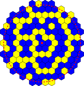
Figure 1. Bernoulli site percolation on the triangular lattice $\mathbb{T}$. Each hexagon of the hexagonal lattice $\mathbb{H}$ represents a site of $\mathbb{T}$, and is colored blue ($t(v)=0$) or yellow ($t(v)=1$). Here, the first-passage time $c_{6}=2$.

Theorem 1 ([28]).

Under the critical Bernoulli FPP measure $\mathbf{P}_{1/2}$ on $\mathbb{T}$,

$$\lim_{n\rightarrow\infty}\frac{c_{n}}{\log n}=\frac{1}{2\sqrt{3}\pi}\quad a.s.,$$ (1)

$$\lim_{n\rightarrow\infty}\frac{\mathbf{E}_{1/2}[c_{n}]}{\log n}=\frac{1}{2\sqrt{3}\pi},$$ (2)

$$\lim_{n\rightarrow\infty}\frac{\operatorname{Var}_{1/2}[c_{n}]}{\log n}=\frac{2}{3\sqrt{3}\pi}-\frac{1}{2\pi^{2}},$$ (3)

$$\lim_{n\rightarrow\infty}\frac{a_{0,n}}{\log n}=\frac{1}{\sqrt{3}\pi}\quad\mbox{in probability but not a.s.}$$ (4)

Let us mention that an analogous theorem for critical Bernoulli FPP starting on the boundary was established in [13]. In [9, 15], the authors studied asymptotics for general planar critical FPP. From Theorem 1.6 in [9] (see also (1.13) in [15]), we know that

$$\frac{c_{n}-\mathbf{E}_{1/2}[c_{n}]}{\sqrt{\operatorname{Var}_{1/2}[c_{n}]}}\stackrel{{\scriptstyle d}}{{\longrightarrow}}N(0,1)\quad\mbox{as }n\rightarrow\infty.$$

This combined with (2) and (3) implies that there exists a function $\delta(n)$ with $\delta(n)\rightarrow 0$ as $n\rightarrow\infty$, such that

$$\frac{c_{n}-(1+\delta(n))\log n/(2\sqrt{3}\pi)}{\sqrt{\left(2/(3\sqrt{3}\pi)-1/(2\pi^{2})\right)\log n}}\stackrel{{\scriptstyle d}}{{\longrightarrow}}N(0,1)\quad\mbox{as }n\rightarrow\infty.$$ (5)

We conjecture, but can not prove, that one may choose $\delta\equiv 0$ in (5). Let us point out that the explicit form of the CLT in Corollary 1.2 of [28] should be replaced with a similar weaker form.

In the present paper, we continue our study of Bernoulli FPP on $\mathbb{T}$ from [28]. The main purpose is threefold: to derive exact asymptotics for Bernoulli FPP as $p\searrow p_{c}$, to construct different subsequential limits for $a_{0,n}$ when $p=p_{c}$, to obtain strong law of large numbers for a natural random graph by applying the result for critical Bernoulli FPP. See the next subsection for details.

Throughout this paper, $C$ or $C_{i}$ stands for a positive constant that may change from line to line according to the context.

1.2. Main results

Before stating our main results, we give some basic notation. For $r>0$, let $\mathbb{D}(r)$ denote the Euclidean disc of radius $r$ centered at 0 and $\partial\mathbb{D}(r)$ denote the boundary of $\mathbb{D}(r)$. Write $\mathbb{D}:=\mathbb{D}(1)$. For $v\in\mathbb{V}$, let $B(v,r)$ denote the set of hexagons of $\mathbb{\mathbb{H}}$ that are contained in $v+\mathbb{D}(r)$. We will sometimes see $B(v,r)$ as a union of these closed hexagons. For $B(v,r)$, denote by $\partial B(v,r)$ its topological boundary. Write $B(r):=B(0,r)$ and $T(0,\partial B(r)):=T(0,\mathbb{C}\backslash B(r))$.

Recall the standard coupling of the percolation measures $\mathbf{P}_{p},0\leq p\leq 1$: Take i.i.d. random variables $U_{v}$ for each site $v$ of $\mathbb{V}$, with $U_{v}$ uniformly distributed on $[0,1]$. We denote the underlying probability measure by $\mathbf{P}$, the corresponding expectation by $\mathbf{E}$, and the space of configurations by $([0,1]^{\mathbb{V}},\mathscr{F})$, where $\mathscr{F}$ is the cylinder $\sigma$-field on $[0,1]^{\mathbb{V}}$. For each $p$, we obtain the measure $\mathbf{P}_{p}$ by declaring each site $v$ to be $p$-open ($t(v)=0$) if $U_{v}\leq p$, and $p$-closed ($t(v)=1$) otherwise. Let $\mathbf{E}_{p}$ denote the expectation with respect to $\mathbf{P}_{p}$. It is well known that almost surely for each $p>1/2$, there is a unique infinite open cluster, denoted by $\mathcal{C}_{\infty}=\mathcal{C}_{\infty}(p)$. Under the coupling measure $\mathbf{P}$, denote by $T_{p}(\cdot,\cdot)$ the first-passage time between two site sets with respect to the parameter $p$.

Let $L(p)$ denote the correlation length that will be defined in Section 2.

We use the standard notation to express that two quantities are asymptotically equivalent. Given two positive functions $f$ and $g$, we write $f\asymp g$ if there are constants $0<C_{1}<C_{2}<\infty$ such that $C_{1}g\leq f\leq C_{2}g$.

1.2.1. Near-critical behavior: supercritical phase

The following theorem roughly says that $T_{p}(0,\mathcal{C}_{\infty}(p))$ is well-approximated by $T_{1/2}(0,\partial B(L(p)))$ under the coupling measure $\mathbf{P}$.

Theorem 2.

There exists some absolute constant $C>0$, such that for all $p>1/2$,

$$\mathbf{E}|T_{p}(0,\mathcal{C}_{\infty}(p))-T_{1/2}(0,\partial B(L(p)))|\leq C,$$ (6)

$$|\operatorname{Var}_{p}[T(0,\mathcal{C}_{\infty})]-\operatorname{Var}_{1/2}[T(0,\partial B(L(p)))]|\leq C.$$ (7)

Assume $p>1/2$, it is easy to show that

$$\lim_{n\rightarrow\infty}c_{n}=T(0,\mathcal{C}_{\infty})\quad\mbox{$\mathbf{P}_{p}$-a.s.},~{}~{}\lim_{n\rightarrow\infty}\mathbf{E}_{p}[c_{n}]=\mathbf{E}_{p}[T(0,\mathcal{C}_{\infty})],~{}~{}\lim_{n\rightarrow\infty}\mathbf{E}_{p}[a_{0,n}]=2\mathbf{E}_{p}[T(0,\mathcal{C}_{\infty})].$$

Zhang [30] proved analogous result for general supercritical FPP on $\mathbb{Z}^{d}$ with $F(0)>p_{c}$. Using Theorem 1 and Theorem 2, we obtain exact asymptotics for $T_{p}(0,\mathcal{C}_{\infty}(p))$ as $p\searrow 1/2$.

Corollary 1.

Suppose $p>1/2$. We have

$$\lim_{p\searrow 1/2}\frac{T_{p}(0,\mathcal{C}_{\infty}(p))}{-\frac{4}{3}\log(p-1/2)}=\frac{1}{2\sqrt{3}\pi}\quad\mbox{$\mathbf{P}$-a.s.,}$$ (8)

$$\lim_{p\searrow 1/2}\frac{\mathbf{E}_{p}[T(0,\mathcal{C}_{\infty})]}{-\frac{4}{3}\log(p-1/2)}=\frac{1}{2\sqrt{3}\pi},$$ (9)

$$\lim_{p\searrow 1/2}\frac{\operatorname{Var}_{p}[T(0,\mathcal{C}_{\infty})]}{-\frac{4}{3}\log(p-1/2)}=\frac{2}{3\sqrt{3}\pi}-\frac{1}{2\pi^{2}}.$$ (10)

Furthermore, there exists a function $\eta(p)$ with $\eta(p)\rightarrow 0$ as $p\searrow 1/2$, such that

$$\frac{T_{p}(0,\mathcal{C}_{\infty}(p))+(1+\eta(p))\frac{2}{3\sqrt{3}\pi}\log(p-1/2)}{\sqrt{\left(\frac{1}{2\pi^{2}}-\frac{2}{3\sqrt{3}\pi}\right)\frac{4}{3}\log(p-1/2)}}\stackrel{{\scriptstyle d}}{{\longrightarrow}}N(0,1)\quad\mbox{as $p\searrow 1/2$}.$$ (11)

Remark 1.

It is natural to ask what will happen when $p\nearrow 1/2$ for the subcritical Bernoulli FPP. Denote by $\mu(p)$ the corresponding time constant. Chayes, Chayes and Durrett [8] proved that $\mu(p)\asymp 1/L(p)$. This result together with (20) implies that $\mu(p)=(1/2-p)^{4/3+o(1)}$ as $p\nearrow 1/2$. Denote by $\mathcal{B}(p)$ the limit shape in the classical “shape theorem” (see e.g. Section 2 in [2]). It will be proved in [29] that $(1/L(p))\mathcal{B}(p)$ converges to a Euclidean disk as $p\nearrow 1/2$. The proof relies on the scaling limit of near-critical percolation constructed by Garban, Pete and Schramm [11].

1.2.2. Subsequential limits for critical Bernoulli FPP

Notice that in (4), we have convergence of $a_{0,n}/\log n$ only in probability, not almost surely. In fact, to show that the convergence does not occur almost surely, in the proof of Theorem 1.1 in [27], we constructed a random subsequence that converges to one half of the typical limiting value almost surely. Using large deviation estimates on the nesting of CLE₆ loops derived by Miller, Watson and Wilson [17], we get the following theorem. Loosely speaking, it says that one can find many subsequences of sites with different growth rate, growing unusually quickly or slowly.

Theorem 3.

Let $\nu_{1}$ be the constant defined in Section 4. $\mathbf{P}_{1/2}$-almost surely, for each $\nu\in[0,\nu_{1}]$, there exists a random subsequence $\{n_{i}:i\geq 1\}$ depending on $\nu$, such that

$$\lim_{i\rightarrow\infty}\frac{a_{0,n_{i}}}{\log n_{i}}=\frac{1}{2\sqrt{3}\pi}+\nu.$$ (12)

Let us mention that $\nu_{1}>1/(2\sqrt{3}\pi)$; one can derive more accurate approximation of $\nu_{1}$ from its definition. Note that (1) implies that $\liminf_{n\rightarrow\infty}a_{0,n}/\log n\geq 1/(2\sqrt{3}\pi)$ a.s. For the $\limsup$ we propose the following question.

Question 1.

Show that under the measure $\mathbf{P}_{1/2}$,

$$\limsup_{n\rightarrow\infty}\frac{a_{0,n}}{\log n}=\frac{1}{2\sqrt{3}\pi}+\nu_{1}\quad\mbox{a.s.}$$

Question 2 below is a discrete analog of Lemma 3.2 of [17], and is related to Question 1.

Question 2.

Suppose $\nu\geq 0$. Show that for all functions $\delta(n)$ decreasing to 0 sufficiently slowly as $n\rightarrow\infty$, we have

$$\left\{\begin{aligned} &\mathbf{P}_{1/2}\left[\nu\leq\frac{c_{n}}{\log n}\leq\nu+\delta(n)\right]=n^{-\gamma(\nu)+o(1)},&\mbox{for }\nu>0,\\ &\mathbf{P}_{1/2}\left[\frac{\delta(n)}{2}\leq\frac{c_{n}}{\log n}\leq\delta(n)\right]=n^{-5/48+o(1)},&\mbox{for }\nu=0.\end{aligned}\right.$$

Remark 2.

Lemma 16 implies that the left hand side of the above equation is not smaller than $n^{-\gamma(\nu)+o(1)}$. The remaining task is to bound it in the other direction.

Note that $5/48$ in the above equation is the value of 1-arm exponent (see e.g. Theorem 21 of [18]). It is clear that

$$\mathbf{P}_{1/2}[c_{n}=0]=(1/2)\mathbf{P}_{1/2}[\mathcal{A}_{1}(1,n)]=n^{-5/48+o(1)}.$$

(See Section 2 for the definition of 1-arm event $\mathcal{A}_{1}(1,n)$.) Proposition 18 of [18] concerns arms with “defects” (i.e. sites of the opposite color), and implies that for each fixed number $d\in\mathbb{N}$,

$$\mathbf{P}_{1/2}[c_{n}\leq d]\asymp(1+\log n)^{d}\mathbf{P}_{1/2}[\mathcal{A}_{1}(1,n)]=n^{-5/48+o(1)}.$$

1.2.3. Application to cluster graph

In this section, we shall introduce a model called cluster graph. It is a natural object constructed from critical percolation. Then we give an application of the limit theorem for critical Bernoulli FPP to this model.

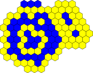
Figure 2. The three open (blue) clusters on the left belong to the same component of cluster graph. The two open clusters on the right are neighbors and belong to a finite component containing only the two clusters.

Cluster graph. Benjamini [4] studied some random metric spaces modeled by graphs. Based on the bond percolation on $\mathbb{Z}^{d}$, in Section 10.2 of [4] he defined a random graph called Contracting Clusters of Critical Percolation (CCCP) by the following rule: Contract each open cluster into a single vertex and define a new edge between the clusters $\mathcal{C},\mathcal{C}^{\prime}$ for every closed edge that connects them in $\mathbb{Z}^{d}$. Similarly, let us define cluster graph based on critical site percolation on $\mathbb{T}$: Contract each open cluster into a single vertex and define a new edge between any pair of clusters $\mathcal{C},\mathcal{C}^{\prime}$ if there exists a closed hexagon touching both of $\mathcal{C}$ and $\mathcal{C}^{\prime}$. Unlike Benjamini’s CCCP which is almost surely a connected multi-graph, our cluster graph is a simple graph and has infinitely many components almost surely. See Figure 2. We embed the cluster graph in the plane in a natural way: Each open cluster is viewed as a vertex of the cluster graph. One may imagine open clusters as islands and closed clusters as lakes, so one cannot cross the water of width larger than the diameter of one hexagon.

Proposition 1.

Cluster graph has a unique infinite component almost surely, denoted by $\mathscr{C}$. There exists a constant $C>0$, such that for any $k\geq 1$,

$$\mathbf{P}_{1/2}[\operatorname{dist}(0,\mathscr{C})\geq k]\leq\exp(-Ck),$$ (13)

where $\operatorname{dist}(\cdot,\cdot)$ denotes Euclidean distance.

To state the following theorem, we need some notation. Let $D(\cdot,\cdot)$ denote the graph distance in the cluster graph. For $n\in\mathbb{N}$, denote by $\mathcal{C}_{n}$ the innermost open cluster surrounding $B(n)$. Let $\mathcal{C}_{0}$ be the open cluster containing 0. Note that if 0 is closed, $\mathcal{C}_{0}=\emptyset$. Using (1), we derive the following strong law of large numbers for the graph distance in cluster graph.

Theorem 4.

Under the conditional probability measure $\mathbf{P}_{1/2}[\cdot|\mathcal{C}_{0}\in\mathscr{C}]$,

$$\lim_{n\rightarrow\infty}\frac{D(\mathcal{C}_{0},\mathcal{C}_{n})}{\log n}=\frac{1}{2\sqrt{3}\pi}\quad\mbox{a.s.}$$

It is worth mentioning another application of critical Bernoulli FPP to loop graph defined below. We will just state the result without giving the proof. We note that the proof is very similar to that for cluster graph.

Loop graph. It is well known that Camia and Newman [7] proved that the scaling limit of cluster boundaries of critical site percolation on $\mathbb{T}$ is CLE₆. Several properties of this scaling limit are established; the third item in Theorem 2 of [7] was called “finite chaining” property in Proposition 2.7 in [10]. That is, for the full-plane CLE₆, almost surely any two loops are connected by a finite path of touching loops. It is natural to define a discrete version of this notion. Similarly to cluster graph, for critical site percolation on $\mathbb{T}$, we contract each cluster boundary loop into a single vertex and define a new edge between any pair of loops $\mathcal{L},\mathcal{L}^{\prime}$ if there exists a hexagon touching both of $\mathcal{L}$ and $\mathcal{L}^{\prime}$. Then we get a random graph called loop graph, whose vertices correspond to cluster boundary loops.

Let $D_{l}(\cdot,\cdot)$ denote the graph distance in the loop graph. For $n\in\mathbb{N}$, denote by $\mathcal{L}_{n}$ the innermost cluster boundary loop surrounding $\mathbb{D}(n)$. Let $\mathcal{L}_{0}$ be the innermost cluster boundary loop surrounding 0.

Similarly to cluster graph, loop graph also has a unique infinite component almost surely, denoted by $\mathscr{C}_{l}$. Moreover, under $\mathbf{P}_{1/2}[\cdot|\mathcal{L}_{0}\in\mathscr{C}_{l}]$,

$$\lim_{n\rightarrow\infty}\frac{D_{l}(\mathcal{L}_{0},\mathcal{L}_{n})}{\log n}=\frac{1}{\sqrt{3}\pi}\quad\mbox{a.s.}$$

2. Notation and preliminaries

Our proofs rely heavily on critical and near-critical percolation. In this section we collect some results that are needed.

A circuit is a path $(v_{1},\ldots,v_{n})$ with $n\geq 3$, such that $v_{1}$ and $v_{n}$ are neighbors. Note that the bonds $(v_{1},v_{2}),\ldots,(v_{n},v_{1})$ of the circuit form a Jordan curve, and sometimes the circuit is viewed as this curve. For a circuit $\mathcal{C}$, define

$$\overline{\mathcal{C}}:=\mathcal{C}\cup\mbox{ interior sites of }\mathcal{C}.$$

If $W$ is a set of sites, then its (external) site boundary is

$$\Delta W:=\{v:v\notin W\mbox{ but $v$ is adjacent to $W$}\}.$$

Given $\varepsilon\in(0,1)$ and $p\in(1/2,1]$, we define the correlation length (or characteristic length) by

$$L_{\varepsilon}(p):=\min\{n\in\mathbb{N}:\mathbf{P}_{p}[\mbox{there is an open horizontal crossing of $[0,n]^{2}$}]\geq 1-\varepsilon\},$$

and by $L_{\varepsilon}(p):=L_{\varepsilon}(1-p)$ for $p<1/2$. We will take the convention $L_{\varepsilon}(1/2)=\infty$.

For two positive functions $f$ and $g$ from a set $\mathcal{X}$ to $(0,\infty)$, we write $f(x)\asymp g(x)$ to indicate that $f(x)/g(x)$ is bounded away from 0 and $\infty$, uniformly in $x\in\mathcal{X}$. It is well known (see e.g. [18]) that there exists $\varepsilon_{0}>0$ such that for all $0<\varepsilon_{1},\varepsilon_{2}\leq\varepsilon_{0}$ we have $L_{\varepsilon_{1}}(p)\asymp L_{\varepsilon_{2}}(p)$. For simplicity we will write $L(p):=L_{\varepsilon_{0}}(p)$ for the entire paper.

For $1\leq r\leq R$ and $v\in\mathbb{V}$, define annuli

$$A(v;r,R):=B(v,R)\backslash B(v,r),~{}~{}A(r,R):=A(0;r,R).$$

The so-called arm events play a central role in studying near-critical percolation. A color sequence $\sigma$ is a sequence $(\sigma_{1},\sigma_{2},\dots,\sigma_{k})$ of “blue” and “yellow” of length $k$. We write 0 and 1 for blue and yellow, respectively. We identify two sequences if they are the same up to a cyclic permutation. For an annulus $A(v;r,R)$, we denote by $\mathcal{A}_{\sigma}(v;r,R)$ the event that there exist $|\sigma|=k$ disjoint monochromatic paths called arms in $A(v;r,R)$ connecting the two boundary pieces of $A(v;r,R)$, whose colors are those prescribed by $\sigma$, when taken in counterclockwise order.

For simplicity, for any $r\geq 1$, we let $\mathcal{A}_{\sigma}(v;r,r)$ be the entire sample space $\Omega$. Write $\mathcal{A}_{\sigma}(r,R)=\mathcal{A}_{\sigma}(0;r,R)$ and $\mathcal{A}_{1}=\mathcal{A}_{(0)}$, $\mathcal{A}_{2}=\mathcal{A}_{(01)}$, $\mathcal{A}_{4}=\mathcal{A}_{(0101)}$, $\mathcal{A}_{6}=\mathcal{A}_{(011011)}$.

Let $\mathcal{O}(r,R)$ denote the event that there exists a blue circuit surrounding 0 in $A(r,R)$. Note that $\mathcal{O}(r,R)=\mathcal{A}_{(1)}^{c}(r,R)$.

We assume that the reader is familiar with the FKG inequality (see Lemma 13 in [18] for generalized FKG), the BK (van den Berg-Kesten) inequality, and the RSW (Russo-Seymour-Welsh) technology. Here we collect some classical results in near-critical percolation that will be used. See e.g. [18, 25] and Section 2.2 in [5].

1. A priori bounds for arm events: For any color sequence $\sigma$, there exist $C_{1}(|\sigma|)$, $C_{2}(|\sigma|)$, $\alpha(|\sigma|)$, $\beta(|\sigma|)>0$ such that for all $1\leq r<R$,

   $$C_{1}\left(\frac{r}{R}\right)^{\alpha}\leq\mathbf{P}_{1/2}[\mathcal{A}_{\sigma}(r,R)]\leq C_{2}\left(\frac{r}{R}\right)^{\beta}.$$

2. Extendability: For any color sequence $\sigma$,

   $$\mathbf{P}_{p}[\mathcal{A}_{\sigma}(r,2R)]\asymp\mathbf{P}_{p}[\mathcal{A}_{\sigma}(r,R)]$$

   uniformly in $p$ and $1\leq r\leq R\leq L(p)$.

3. Quasi-multiplicativity: For any color sequence $\sigma$, there exists $C(|\sigma|)>0$, such that

   $$C\mathbf{P}_{p}[\mathcal{A}_{\sigma}(r_{1},r_{2})]\mathbf{P}_{p}[\mathcal{A}_{\sigma}(r_{2},r_{3})]\leq\mathbf{P}_{p}[\mathcal{A}_{\sigma}(r_{1},r_{3})]$$

   uniformly in $p$ and $1\leq r_{1}<r_{2}<r_{3}\leq L(p)$.

4. For any color sequence $\sigma$,

   $$\mathbf{P}_{p}[\mathcal{A}_{\sigma}(r,R)]\asymp\mathbf{P}_{1/2}[\mathcal{A}_{\sigma}(r,R)]$$ (14)

   uniformly in $p$ and $1\leq r<R\leq L(p)$.

5. As $p\rightarrow 1/2$,

   $$|p-1/2|(L(p))^{2}\mathbf{P}_{1/2}[\mathcal{A}_{4}(1,L(p))]\asymp 1.$$ (15)

6. Exponential decay with respect to $L(p)$. There are constants $C_{1},C_{2}>0$, such that for all $p>1/2$ and $R\geq L(p)$ (see item (ii) in Section 2.2 of [5]),

   $$\mathbf{P}_{p}[\mathcal{A}_{1}(R,\infty)]\geq 1-C_{1}\exp\left(-C_{2}\frac{R}{L(p)}\right),$$ (16)

   $$\mathbf{P}_{p}[\mathcal{O}(R,2R)]\geq 1-C_{1}\exp\left(-C_{2}\frac{R}{L(p)}\right).$$ (17)

7. There exist constants $\varepsilon,C>0$, such that for all $p$ and $1\leq r<R\leq L(p)$,

   $$\mathbf{P}_{p}[\mathcal{A}_{4}(r,R)]\geq C\left(\frac{r}{R}\right)^{2-\varepsilon}.$$ (18)

8. There exist constants $\varepsilon,C>0$, such that for all $1\leq r<R$,

   $$\mathbf{P}_{1/2}[\mathcal{A}_{6}(r,R)]\leq C\left(\frac{r}{R}\right)^{2+\varepsilon}.$$ (19)

9. When $p\rightarrow 1/2$,

   $$L(p)=|p-1/2|^{-4/3+o(1)}.$$ (20)

It is well known that for a fixed number $j$ of arms, if its color sequence is polychromatic (both colors are present), prescribing it changes the probability only by at most a constant factor. Beffara and Nolin [3] showed that the monochromatic $j$-arm exponent is strictly between the polychromatic $j$-arm and $(j+1)$-arm exponents. The following result was essentially proved, see (2.10) and the inequality just below (3.1) in [3].

Lemma 1 ([3]).

For any polychromatic color sequence $\sigma$, there exist $\varepsilon,C>0$ (depending on $|\sigma|$), such that for all $1\leq m<n$,

$$\mathbf{P}_{1/2}[\mathcal{A}_{(\underbrace{1\ldots 1}_{|\sigma|})}(m,n)]\leq C\left(\frac{n}{m}\right)^{-\varepsilon}\mathbf{P}_{1/2}[\mathcal{A}_{\sigma}(m,n)].$$

We call a continuous map from the circle to $\mathbb{C}$ a loop; the loops are identified up to reparametrization by homeomorphisms of the circle with positive winding. Let $\textrm{d}(\cdot,\cdot)$ denote the uniform metric on loops:

$$\textrm{d}(\gamma_{1},\gamma_{2}):=\inf_{\phi}\sup_{t\in\mathbb{R}/\mathbb{Z}}|\gamma_{1}(t)-\gamma_{2}(\phi(t))|,$$

where the infimum is taken over all homeomorphisms of the circle which have positive winding. The distance between two closed sets of loops is defined by the induced Hausdorff metric as follows:

$$\operatorname{dist}(\mathcal{F},\mathcal{F}^{\prime}):=\inf\{\varepsilon>0:\forall\gamma\in\mathcal{F},\exists\gamma^{\prime}\in\mathcal{F}^{\prime}\mbox{ such that }\textrm{d}(\gamma,\gamma^{\prime})\leq\varepsilon\mbox{ and vice versa}\}.$$ (21)

For critical site percolation on $\mathbb{T}$, we orient a cluster boundary loop counterclockwise if it has blue sites on its inner boundary and yellow sites on its outer boundary, otherwise we orient it clockwise. We say $B(R)$ has monochromatic (blue) boundary condition if all the sites in $\Delta B(R)$ are blue. Based on Smirnov’s celebrated work [23], Camia and Newman [7] showed the following well-known result.

Theorem 5 ([7]).

As $\eta\rightarrow 0$, the collection of all cluster boundaries of critical site percolation on $\eta\mathbb{T}$ in $\mathbb{D}$ with monochromatic boundary conditions converges in distribution, under the topology induced by metric (21), to a probability distribution on collections of continuous nonsimple loops in $\overline{\mathbb{D}}$.

We call the continuum nonsimple loop process in Theorem 5 the conformal loop ensemble CLE₆ in $\overline{\mathbb{D}}$. General CLE_κ for $8/3<\kappa<8$ is the canonical conformally invariant measure on countably infinite collections of noncrossing loops in a simply connected planar domain, see [21, 22]. We denote by $\mathbb{P}$ the probability measure of CLE₆ in $\overline{\mathbb{D}}$ and by $\mathbb{E}$ the expectation with respect to $\mathbb{P}$.

Given an annulus $A(r,R)$, define

$$\rho(r,R) :=\mbox{the maximal number of disjoint yellow circuits surrounding 0 in }A(r,R),$$

$$N(r,R) :=\mbox{the number of cluster boundary loops surrounding 0 in $A(r,R)$}.$$

The following elementary proposition is crucial for enabling us to use the scaling limit of critical site percolation on $\mathbb{T}$ to derive explicit limit theorem for our special FPP model. Note that item (i) implies item (ii) immediately.

Proposition 2 (Proposition 2.4 in [28]).

Consider Bernoulli FPP on $\mathbb{T}$ with parameter $p$. Suppose $1\leq r<R$. Then we have:

• $T(\partial B(r),\partial B(R))=\rho(r,R)$.

• There exist $T(\partial B(r),\partial B(R))$ disjoint yellow circuits surrounding 0 in $A(r,R)$, such that for any geodesic $\gamma$ from $\partial B(r)$ to $\partial B(R)$ in $A(r,R)$, each closed site in $\gamma$ is in one of these circuits, with different closed sites lying in different circuits.

• Assume that $p=1/2$ and $B(R)$ has monochromatic boundary condition. Then $T(\partial B(r),\partial B(R))$ has the same distribution as $N(r,R)$.

For $1\leq r<R$, denote by $S(r,R)$ (resp. $S_{r}$) the maximal number of disjoint yellow circuits surrounding 0 and intersecting $A(r,R)$ (resp. $\partial B(r)$).

Lemma 2.

There exist constants $C_{1},\ldots,C_{4}>0$ and $K>1$, such that for all $1\leq r<R$ and $x\geq K\log_{2}(R/r)$,

$$\mathbf{P}_{1/2}[\rho(r,R)\geq x]\leq C_{1}\exp(-C_{2}x),$$ (22)

$$\mathbf{P}_{1/2}[S(r,R)\geq x]\leq C_{3}\exp(-C_{4}x).$$ (23)

Hence, there exists a constant $C_{5}>0$, such that for all $1\leq r\leq R/2$,

$$\mathbf{E}_{1/2}[S^{4}(r,R)]\leq C_{5}\log^{4}(R/r).$$

Proof.

Combining item (i) in Proposition 2 and Lemma 2.5 in [28], we get (22).

Using RSW, FKG and BK inequality, it is easy to prove that there exists a constant $C_{6}>0$, such that for all $r\geq 1$ and $x\geq 1$,

$$\mathbf{P}_{1/2}[S_{r}\geq x]\leq\exp(-C_{6}x).$$

Since $S(r,R)\leq\rho(r,R)+S_{r}+S_{R}$, the above inequality and (22) imply (23) immediately. ∎

3. Supercritical regime

In this section, we will prove Theorem 2 and Corollary 1. We first introduce Russo’s formula for random variables in Section 3.1. This formula plays a central role in the proof of Theorem 2, since it allows us to study how the expectation of a random variable varies when the percolation parameter $p$ varies. Then we prove (6) and (7) in Sections 3.2 and 3.3, respectively. The proof of Corollary 1 is given in Section 3.4.

For convenience, in the proofs of this section we always assume without loss of generality that $L(p)$ is large, say, $L(p)\geq 20$. So we suppose that $p\leq p_{0}$ for some fixed $p_{0}\in(1/2,1)$. It is easy to see by (16) that $\mathbf{E}_{p}[T^{2}(0,\mathcal{C}_{\infty})]$ is uniformly bounded for $p\in[p_{0},1]$, which implies that (6) and (7) hold for $p\in[p_{0},1]$ immediately.

3.1. Russo’s formula

We begin with some notation. Given a percolation configuration $\omega=\{\omega(u)\}_{u\in\mathbb{V}}\in\Omega$ and a site $v\in\mathbb{V}$, let

$$\omega^{v}(u):=\left\{\begin{aligned} &\omega(u)&\mbox{ if }u\neq v,\\ &0&\mbox{if }u=v.\end{aligned}\right.\quad\omega_{v}(u):=\left\{\begin{aligned} &\omega(u)&\mbox{ if }u\neq v,\\ &1&\mbox{if }u=v.\end{aligned}\right.$$

(Note that in the percolation literature $\omega^{v}$ usually means that we set $v$ to be 1; here we adopt the above setting since, for our Bernoulli FPP, a site is open when it takes the value 0, while in the percolation literature, a site is open usually means that the site takes the value 1.) For a random variable $X=X(\omega)$, define the increment of $X$ at $v$ by

$$\delta_{v}X(\omega):=X(\omega^{v})-X(\omega_{v}).$$

Lemma 3 (Russo’s formula, see e.g. Theorem 2.32 in [12]).

Let $X$ be a random variable which is defined in terms of the states of only finitely many sites of $\mathbb{T}$. Then

$$\frac{d}{dp}\mathbf{E}_{p}[X]=\sum_{v\in\mathbb{V}}\mathbf{E}_{p}[\delta_{v}X].$$

3.2. Study of the mean

Suppose $p>1/2$. For simplicity of notation, let $T(p):=T(0,\partial B(L(p)))$. To prove (6), we write

$$\mathbf{E}|T_{1/2}(0,\partial B(L(p)))-T_{p}(0,\mathcal{C}_{\infty}(p))|$$

$$\leq\mathbf{E}|T_{1/2}(0,\partial B(L(p)))-T_{p}(0,\partial B(L(p)))|+\mathbf{E}|T_{p}(0,\partial B(L(p)))-T_{p}(0,\mathcal{C}_{\infty}(p))|$$

$$=\{\mathbf{E}_{1/2}[T(p)]-\mathbf{E}_{p}[T(p)]\}+\{\mathbf{E}_{p}[T(0,\mathcal{C}_{\infty})]-\mathbf{E}_{p}[T(p)]\}.$$ (24)

We will bound the two terms on the right-hand side of (24) separately, starting with the first term.

Lemma 4.

There is a constant $C>0$ such that for all $p>1/2$,

$$\mathbf{E}_{1/2}[T(p)]-\mathbf{E}_{p}[T(p)]\leq C.$$

Proof.

For each $v\in B(L(p))$, define the event

$$\mathcal{E}_{v}:=\{\mbox{for $\omega_{v}$, $\exists$ a geodesic $\gamma$ from 0 to $\partial B(L(p))$ in $B(L(p))$ with $v\in\gamma$}\}.$$

By Lemma 3, applying Russo’s formula to $T(p)$ for $\mathbf{E}_{h}$, where $1/2\leq h\leq p$, one obtains

$$-\frac{d}{dh}\mathbf{E}_{h}[T(p)]=-\sum_{v\in B(L(p))}\mathbf{E}_{h}[\delta_{v}T(p)]=\sum_{v\in B(L(p))}\mathbf{P}_{h}[\mathcal{E}_{v}].$$ (25)

Now let us show that there is a universal constant $C_{1}>0$, such that for $v\in A(2,L(p))$,

$$\mathbf{P}_{h}[\mathcal{E}_{v}]\leq C_{1}\mathbf{P}_{1/2}[\mathcal{A}_{4}(1,|v|)].$$ (26)

Take $K=K(v)=\lfloor\log_{2}|v|\rfloor$. We start by analyzing the case that $v$ is far from the boundary of $B(L(p))$, that is, $v\in A(2,L(p)/2)$. Define the event

$$\mathcal{F}_{v}:=\{\exists~{}r\mbox{ such that $1\leq r\leq 2^{K}$ and $\mathcal{A}_{4}(v;1,r)\cap\mathcal{A}_{(1111)}(v;r,2^{K})$ occurs}\}.$$

Note that $\mathcal{A}_{4}(v;1,2^{K})\subset\mathcal{F}_{v}$ since we have set $\mathcal{A}_{(1111)}(v;2^{K},2^{K})=\Omega$.

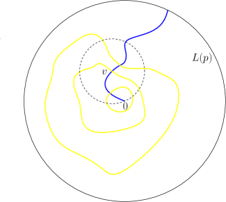
Figure 3. For $v\in A(2,L(p)/2)$, the event $\mathcal{E}_{v}\subset\mathcal{F}_{v}$.

Assume that $v\in A(2,L(p)/2)$. By item (ii) in Proposition 2, we have $\mathcal{E}_{v}\subset\mathcal{F}_{v}$. See Figure 3. Let us bound the probability of the event $\mathcal{F}_{v}$. By considering the smallest $r$ satisfying $\mathcal{F}_{v}$ with $2^{i}\leq r\leq 2^{i+1}$, we get that there exist universal constants $\varepsilon,C_{2},\dots,C_{5}>0$ such that

$$\mathbf{P}_{h}[\mathcal{F}_{v}] \leq\sum_{i=0}^{K-1}\mathbf{P}_{h}[\mathcal{A}_{4}(v;1,2^{i})]\mathbf{P}_{h}[\mathcal{A}_{(1111)}(v;2^{i+1},2^{K})]$$

$$\leq\sum_{i=0}^{K-1}C_{2}\mathbf{P}_{1/2}[\mathcal{A}_{4}(1,2^{i})]\mathbf{P}_{1/2}[\mathcal{A}_{(1111)}(2^{i+1},2^{K})]~{}~{}\mbox{by (\ref{e7})}$$

$$\leq\sum_{i=0}^{K-1}C_{3}\mathbf{P}_{1/2}[\mathcal{A}_{4}(1,2^{i})]\mathbf{P}_{1/2}[\mathcal{A}_{4}(2^{i+1},2^{K})]2^{-\varepsilon(K-i-1)}~{}~{}\mbox{by Lemma \ref{l4}}$$

$$\leq\sum_{i=0}^{K-1}C_{4}\mathbf{P}_{1/2}[\mathcal{A}_{4}(1,2^{K})]2^{-\varepsilon(K-i-1)}~{}~{}\mbox{ by quasi-multiplicativity}$$

$$\leq C_{5}\mathbf{P}_{1/2}[\mathcal{A}_{4}(1,|v|)]~{}~{}\mbox{by extendability.}$$ (27)

Then for $v\in A(2,L(p)/2)$, we get (26) from (27) since $\mathcal{E}_{v}\subset\mathcal{F}_{v}$.

Now we bound $\mathbf{P}_{h}[\mathcal{E}_{v}]$ for the sites $v$ which are close to the boundary of $B(L(p))$, that is, $v\in A(L(p)/2,L(p))$. Let us mention that in the proof of Lemma 4, one can avoid analyzing this case by introducing an intermediate measure $\widetilde{\mathbf{P}}_{h}$ satisfying $\widetilde{\mathbf{P}}_{h}|_{A(L(p)/2,L(p))}=\mathbf{P}_{1/2}|_{A(L(p)/2,L(p))}$ and $\widetilde{\mathbf{P}}_{h}|_{B(L(p)/2)}=\mathbf{P}_{h}|_{B(L(p)/2)}$. However, in the study of the variance in Section 3.3 we will need to handle the boundary issue. So we give the analysis here, and will use it in Section 3.3.

Assume that $v\in A(L(p)/2,L(p))$ and $1<r\leq|v|$. Define the event

$$\widehat{\mathcal{A}}_{4}(v;1,r):= \{\mbox{$\exists$ four alternating arms from $v$ to $\partial(B(v,r)\cap B(L(p)))$ in $B(v,r)\cap B(L(p))$.}$$

$$\mbox{Furthermore, three of them are from $v$ to $\partial B(v,r)$, with color sequence $(101)$}\}.$$

When $v$ touches $\partial B(L(p))$, we just interpret $\widehat{\mathcal{A}}_{4}(v;1,r)$ as the event that there exist three arms from $v$ to $\partial B(v,r)$ in $B(v,r)\cap B(L(p))$, with color sequence $(101)$. It is clear that when $r\leq L(p)-|v|$, we have $\widehat{\mathcal{A}}_{4}(v;1,r)=\mathcal{A}_{4}(v;1,r)$.

By using the fact that the polychromatic half-plane 3-arm exponent is 2, which is larger than the 4-arm exponent, it is standard to show that there is some universal constant $C_{6}>0$, such that

$$\mathbf{P}_{h}[\widehat{\mathcal{A}}_{4}(v;1,r)]\leq C_{6}\mathbf{P}_{1/2}[\mathcal{A}_{4}(1,r)].$$ (28)

Similarly to the event $\mathcal{F}_{v}$, for $v\in A(L(p)/2,L(p))$ we define the event

$$\widehat{\mathcal{F}}_{v}:=\{\exists~{}r\mbox{ such that $1\leq r\leq 2^{K}$ and $\widehat{\mathcal{A}}_{4}(v;1,r)\cap\mathcal{A}_{(1111)}(v;r,2^{K})$ occurs}\}.$$

Suppose that $v\in A(L(p)/2,L(p))$. Using item (ii) in Proposition 2, we have $\mathcal{E}_{v}\subset\widehat{\mathcal{F}}_{v}$. By considering the smallest $r$ satisfying $\widehat{\mathcal{F}}_{v}$ with $2^{i}\leq r\leq 2^{i+1}$, we obtain that

$$\mathbf{P}_{h}[\widehat{\mathcal{F}}_{v}] \leq\sum_{i=0}^{K-1}\mathbf{P}_{h}[\widehat{\mathcal{A}}_{4}(v;1,2^{i})]\mathbf{P}_{h}[\mathcal{A}_{(1111)}(v;2^{i+1},2^{K})]$$

$$\leq\sum_{i=0}^{K-1}C_{7}\mathbf{P}_{1/2}[\mathcal{A}_{4}(1,2^{i})]\mathbf{P}_{1/2}[\mathcal{A}_{4}(2^{i+1},2^{K})]2^{-\varepsilon(K-i-1)}~{}~{}\mbox{by (\ref{e71}), (\ref{e7}) and Lemma \ref{l4}}$$

$$\leq C_{8}\mathbf{P}_{1/2}[\mathcal{A}_{4}(1,|v|)]~{}~{}\mbox{by the proof of (\ref{e70}).}$$ (29)

Then for $v\in A(L(p)/2,L(p))$, we derive (26) from (29) since $\mathcal{E}_{v}\subset\widehat{\mathcal{F}}_{v}$. This combined with the above argument for $v\in A(2,L(p)/2)$ ends the proof of (26).

Take $M$ such that $2^{M}\leq L(p)<2^{M+1}$. We have

$$\sum_{v\in A(2,L(p))}\mathbf{P}_{h}[\mathcal{E}_{v}] \leq\sum_{i=1}^{M}\sum_{v\in A(2^{i},2^{i+1})}C_{1}\mathbf{P}_{1/2}[\mathcal{A}_{4}(1,|v|)]~{}~{}\mbox{ by (\ref{e68})}$$

$$\leq\sum_{i=1}^{M}C_{9}4^{i}\mathbf{P}_{1/2}[\mathcal{A}_{4}(1,2^{i})]$$

$$\leq\sum_{i=1}^{M}C_{10}4^{i}\frac{\mathbf{P}_{1/2}[\mathcal{A}_{4}(1,L(p))]}{\mathbf{P}_{1/2}[\mathcal{A}_{4}(2^{i},L(p))]}~{}~{}\mbox{ by quasi-multiplicativity}$$

$$\leq\sum_{i=1}^{M}C_{11}2^{-\varepsilon(M-i)}(L(p))^{2}\mathbf{P}_{1/2}[\mathcal{A}_{4}(1,L(p))]~{}~{}\mbox{ by (\ref{e9})}$$

$$\leq C_{12}(L(p))^{2}\mathbf{P}_{1/2}[\mathcal{A}_{4}(1,L(p))].$$ (30)

Finally, by integrating (25) from $1/2$ to $p$ and using (30) and (15), we have

$$\mathbf{E}_{1/2}[T(p)]-\mathbf{E}_{p}[T(p)]\leq C_{13}+C_{12}(p-1/2)(L(p))^{2}\mathbf{P}_{1/2}[\mathcal{A}_{4}(1,L(p))]\leq C,$$

which completes the proof. ∎

Remark 3.

Let us mention that without using Lemma 1 one can derive (27) by a weaker result. It is noted just below (2.8) of [3], by using a theorem from Reimer (Theorem 3 in [3]), one easily obtains $\mathbf{P}_{1/2}[\mathcal{A}_{(111111)}(2^{i+1},2^{K})]\leq\mathbf{P}_{1/2}[\mathcal{A}_{(011111)}(2^{i+1},2^{K})]$. This inequality together with $\mathbf{P}_{1/2}[\mathcal{A}_{6}(2^{i+1},2^{K})]\leq\mathbf{P}_{1/2}[\mathcal{A}_{4}(2^{i+1},2^{K})]2^{-\varepsilon(K-i-1)}$ enables us to derive (27) by a more complicated argument. We will not give the details here.

Let us now bound the second term of (24).

Lemma 5.

There is a constant $C>0$ such that for all $p>1/2$,

$$\mathbf{E}_{p}[T(0,\mathcal{C}_{\infty})-T(p)]\leq C.$$

Proof.

By (16), (17) and FKG, there exist $C_{1},C_{2}>0$, such that for all $p>1/2$ and $R\geq L(p)$,

$$\mathbf{P}_{p}[\mathcal{O}(R,2R)\cap\mathcal{A}_{1}(R,\infty)]\geq 1-C_{1}\exp\left(-C_{2}\frac{R}{L(p)}\right).$$ (31)

For $j\geq 0$, define the event

$$\mathcal{W}_{j}:=\{j=\min\{i\geq 0:\mathcal{O}(2^{i}L(p),2^{i+1}L(p))\cap\mathcal{A}_{1}(2^{i}L(p),\infty)\mbox{ occurs}\}\}.$$

Then we have

$$\mathbf{E}_{p}[T(0,\mathcal{C}_{\infty})-T(p)]$$

$$\leq\sum_{j=0}^{\infty}\mathbf{E}_{p}[S(L(p),2^{j+1}L(p))\mathbf{1}_{\mathcal{W}_{j}}]$$

$$\leq\sum_{j=0}^{\infty}\left\{\mathbf{E}_{p}[S^{2}(L(p),2^{j+1}L(p))]\right\}^{1/2}\left\{\mathbf{P}_{p}[\mathcal{W}_{j}]\right\}^{1/2}~{}~{}\mbox{ by Cauchy-Schwarz inequality}$$

$$\leq\sum_{j=0}^{\infty}C_{3}(j+1)\exp(-C_{2}2^{j})~{}~{}\mbox{ by (\ref{e12}) and Lemma \ref{l10}},$$

which concludes the proof. ∎

Combining Lemmas 4 and 5, the two terms on the right-hand side of (24) are bounded, and we obtain (6).

3.3. Study of the variance

Suppose $p>1/2$. Recall $T(p):=T(0,\partial B(L(p)))$. Let $J(p):=\lceil\log_{2}(L(p))\rceil+1$. To prove (7), we write

$$|\operatorname{Var}_{1/2}[T(p)]-\operatorname{Var}_{p}[T(0,\mathcal{C}_{\infty})]|$$

$$\leq|\operatorname{Var}_{1/2}[T(p)]-\operatorname{Var}_{p}[T(p)]|+|\operatorname{Var}_{p}[T(0,\mathcal{C}_{\infty})]-\operatorname{Var}_{p}[T(0,\mathcal{C}_{J(p)})]|$$

$$\quad+|\operatorname{Var}_{p}[T(0,\mathcal{C}_{J(p)})]-\operatorname{Var}_{p}[T(p)]|,$$ (32)

where $\mathcal{C}_{J(p)}$ is an open circuit surrounding 0 and is defined in Section 3.3.2. In Sections 3.3.1, 3.3.2 and 3.3.3, we will bound the three terms on the right-hand side of (32), respectively. Let us now focus on the first term.

3.3.1. Bound on $|\operatorname{Var}_{1/2}[T(p)]-\operatorname{Var}_{p}[T(p)]|$

Lemma 6.

There is a constant $C>0$ such that for all $p>1/2$,

$$|\operatorname{Var}_{1/2}[T(p)]-\operatorname{Var}_{p}[T(p)]|\leq C.$$

Proof.

Similarly to the proof of Lemma 4, we shall use Russo’s formula again, although the proof turns out to be more involved. Recall the definition of the event $\mathcal{E}_{v}$ defined in the proof of Lemma 4. For $1/2\leq h\leq p$, applying Lemma 3, one obtains

$$\frac{d}{dh}\{\mathbf{E}_{h}[T^{2}(p)]-\mathbf{E}_{h}^{2}[T(p)]\}$$

$$=\sum_{v\in B(L(p))}\{\mathbf{E}_{h}[\delta_{v}T^{2}(p)]-2\mathbf{E}_{h}[T(p)]\mathbf{E}_{h}[\delta_{v}T(p)]\}$$

$$=\sum_{v\in B(L(p))}\{\mathbf{E}_{h}[T^{2}(p)(\omega^{v})-T^{2}(p)(\omega_{v})]-2\mathbf{E}_{h}[T(p)]\mathbf{E}_{h}[T(p)(\omega^{v})-T(p)(\omega_{v})]\}$$

$$=\sum_{v\in B(L(p))}\{\mathbf{E}_{h}[\mathbf{1}_{\mathcal{E}_{v}}]+2\mathbf{E}_{h}[\mathbf{1}_{\mathcal{E}_{v}}]\mathbf{E}_{h}[T(p)]-2\mathbf{E}_{h}[\mathbf{1}_{\mathcal{E}_{v}}T(p)(\omega_{v})]\}$$

$$=\sum_{v\in B(L(p))}(1-2h)\mathbf{P}_{h}[\mathcal{E}_{v}]+\sum_{v\in B(L(p))}2\{\mathbf{P}_{h}[\mathcal{E}_{v}]\mathbf{E}_{h}[T(p)]-\mathbf{E}_{h}[\mathbf{1}_{\mathcal{E}_{v}}T(p)]\}.$$ (33)

Unlike the expectation, it is not clear if $\operatorname{Var}_{h}[T(p)]$ is monotonic in $h$. So we need to bound the absolute value of the above derivative. It turns out that the key ingredient is to prove the following claim: For $v\in B(4,L(p))$,

$$\mathbf{E}_{h}[\mathbf{1}_{\mathcal{E}_{v}}T(p)]=\mathbf{P}_{h}[\mathcal{E}_{v}]\mathbf{E}_{h}[T(p)]+O(1)\mathbf{P}_{1/2}[\mathcal{A}_{4}(1,|v|)].$$ (34)

To show the claim (34), we will control the decorrelation of $\mathbf{1}_{\mathcal{E}_{v}}T(p)$ and give the lower and upper bounds of $\mathbf{E}_{h}[\mathbf{1}_{\mathcal{E}_{v}}T(p)]$ separately. We start with some notation. Assume $v\in A(4,L(p)/2)$. Define the events

$$\mathcal{G}_{i}^{-}:=\left\{\begin{aligned} &\{i=\min\{k\geq 1:\mathcal{O}(2^{-k-1}|v|,2^{-k}|v|)\mbox{ occurs}\}\}&\mbox{ if }1\leq i\leq\lfloor\log_{2}|v|\rfloor-1,\\ &\{\forall~{}1\leq k\leq i-1,\mathcal{O}(2^{-k-1}|v|,2^{-k}|v|)\mbox{ does not occur}\}&\mbox{if }i=\lfloor\log_{2}|v|\rfloor.\end{aligned}\right.$$

$$\mathcal{G}_{j}^{+}:=\left\{\begin{aligned} &\{j=\min\{k\geq 1:\mathcal{O}(2^{k}|v|,2^{k+1}|v|)\mbox{ occurs}\}\}&\mbox{ if }1\leq j\leq\lfloor\log_{2}(L(p)/|v|)\rfloor-1,\\ &\{\forall~{}1\leq k\leq j-1,\mathcal{O}(2^{k}|v|,2^{k+1}|v|)\mbox{ does not occur}\}&\mbox{ if }j=\lfloor\log_{2}(L(p)/|v|)\rfloor.\end{aligned}\right.$$

$$\mathcal{G}_{i,j}:=\mathcal{G}_{i}^{-}\cap\mathcal{G}_{j}^{+}.$$

Write $\mathcal{I}=\mathcal{I}(|v|):=\{1,2,\ldots,\lfloor\log_{2}|v|\rfloor\}$ and $\mathcal{J}=\mathcal{J}(p,|v|):=\{1,2,\ldots,\lfloor\log_{2}(L(p)/|v|)\rfloor\}$. By RSW and FKG, it is standard to show that there exist universal $C_{1},C_{2}>0$ such that

$$\exp(-C_{1}(i+j))\leq\mathbf{P}_{h}[\mathcal{G}_{i,j}]\leq\exp(-C_{2}(i+j)).$$ (35)

Let $\widehat{\mathcal{A}}_{4}(v;1,r)$ be the event defined in the proof of Lemma 4. For $v\in B(4,L(p))$, define the event

$$\widetilde{\mathcal{E}}_{v}:=\left\{\begin{aligned} &\{\exists~{}1\leq r\leq|v|/3\mbox{ s.t. $\mathcal{A}_{4}(v;1,r)\cap\mathcal{A}_{(1111)}(v;r,|v|/3)$ occurs}\}&\mbox{if }v\in B(4,L(p)/2),\\ &\{\exists~{}1\leq r\leq|v|/3\mbox{ s.t. $\widehat{\mathcal{A}}_{4}(v;1,r)\cap\mathcal{A}_{(1111)}(v;r,|v|/3)$ occurs}\}&\mbox{if }v\in B(L(p)/2,L(p)).\end{aligned}\right.$$

Note that $\mathcal{E}_{v}\subset\widetilde{\mathcal{E}}_{v}$. Similarly to the proof of (27) and (29), one derives that there is a universal $C_{3}>0$, such that

$$\mathbf{P}_{h}[\widetilde{\mathcal{E}}_{v}]\leq C_{3}\mathbf{P}_{1/2}[\mathcal{A}_{4}(1,|v|)].$$ (36)

For $v\in A(4,L(p)/2)$, write

$$\mathbf{E}_{h}[\mathbf{1}_{\mathcal{E}_{v}}T(p)]=\sum_{i\in\mathcal{I},j\in\mathcal{J}}\mathbf{P}_{h}[\mathcal{G}_{i,j}]\mathbf{E}_{h}[\mathbf{1}_{\mathcal{E}_{v}}T(p)|\mathcal{G}_{i,j}].$$

For convenience, let $T(0,\partial B(r))=0$ if $r\leq\sqrt{3}/2$ and let $T(\partial B(r),\partial B(R))=0$ if $r\geq R$. Observe that conditioned on $\mathcal{G}_{i,j}$, the indicator function $\mathbf{1}_{\mathcal{E}_{v}}$ and $T(0,\partial B(2^{-i-1}|v|))+T(\partial B(2^{j+1}|v|),\partial B(L(p)))$ are independent. Indeed, conditionally on $\mathcal{G}_{i,j}$, we distinguish the following four cases: (1) Suppose that $i\in\mathcal{I}\backslash\{\lfloor\log_{2}|v|\rfloor\}$ and $j\in\mathcal{J}\backslash\{\lfloor\log_{2}(L(p)/|v|)\rfloor\}$. The event $\mathcal{E}_{v}$ is equivalent to the event that for $\omega_{v}$, there exists a geodesic $\gamma$ from an open circuit surrounding 0 in $A(2^{-i-1}|v|,2^{-i}|v|)$ to an open circuit surrounding 0 in $A(2^{j}|v|,2^{j+1}|v|)$, with $v\in\gamma$. So $\mathcal{E}_{v}$ is independent of the configuration outside $A(2^{-i-1}|v|,2^{j+1}|v|)$. In particular, $\mathcal{E}_{v}$ is independent of $T(0,\partial B(2^{-i-1}|v|))+T(\partial B(2^{j+1}|v|),\partial B(L(p)))$. (2) Suppose that $i\in\mathcal{I}\backslash\{\lfloor\log_{2}|v|\rfloor\}$ and $j=\lfloor\log_{2}(L(p)/|v|)\rfloor$. The event $\mathcal{E}_{v}$ is equivalent to the event that for $\omega_{v}$, there exists a geodesic $\gamma$ from an open circuit surrounding 0 in $A(2^{-i-1}|v|,2^{-i}|v|)$ to $\partial B(L(p))$, with $v\in\gamma$. So $\mathcal{E}_{v}$ is independent of $T(0,\partial B(2^{-i-1}|v|))$. (3) Suppose that $i=\lfloor\log_{2}|v|\rfloor$ and $j\in\mathcal{J}\backslash\{\lfloor\log_{2}(L(p)/|v|)\rfloor\}$. The argument for this case is similar to that for the case (2). (4) Suppose that $i=\lfloor\log_{2}|v|\rfloor$ and $j=\lfloor\log_{2}(L(p)/|v|)\rfloor$. Then the observation is trivial since $T(0,\partial B(2^{-i-1}|v|))=T(\partial B(2^{j+1}|v|),\partial B(L(p)))=0$ in this case.

Then we have

$$\mathbf{E}_{h}[\mathbf{1}_{\mathcal{E}_{v}}T(p)]$$

$$\geq\sum_{i\in\mathcal{I},j\in\mathcal{J}}\mathbf{P}_{h}[\mathcal{G}_{i,j}]\mathbf{E}_{h}[\mathbf{1}_{\mathcal{E}_{v}}|\mathcal{G}_{i,j}]\mathbf{E}_{h}[T(0,\partial B(2^{-i-1}|v|))+T(\partial B(2^{j+1}|v|),\partial B(L(p)))]$$

$$\geq\sum_{i\in\mathcal{I},j\in\mathcal{J}}\mathbf{P}_{h}[\mathcal{E}_{v}\mathcal{G}_{i,j}]\{\mathbf{E}_{h}[T(p)]-\mathbf{E}_{h}[S(2^{-i-1}|v|,2^{j+1}|v|)]\}$$

$$\geq\mathbf{P}_{h}[\mathcal{E}_{v}]\mathbf{E}_{h}[T(p)]-\sum_{i\in\mathcal{I},j\in\mathcal{J}}C_{4}(i+j)\mathbf{P}_{h}[\mathcal{E}_{v}\mathcal{G}_{i,j}]~{}~{}\mbox{ by Lemma \ref{l10}}.$$

Since $\mathcal{E}_{v}\subset\widetilde{\mathcal{E}}_{v}$ and $\widetilde{\mathcal{E}}_{v}$ is independent of the event $\mathcal{G}_{i,j}$, we have

$$\mathbf{E}_{h}[\mathbf{1}_{\mathcal{E}_{v}}T(p)] \geq\mathbf{P}_{h}[\mathcal{E}_{v}]\mathbf{E}_{h}[T(p)]-\sum_{i\in\mathcal{I},j\in\mathcal{J}}C_{4}(i+j)\exp(-C_{2}(i+j))\mathbf{P}_{h}[\widetilde{\mathcal{E}}_{v}]~{}~{}\mbox{ by (\ref{e20})}$$

$$\geq\mathbf{P}_{h}[\mathcal{E}_{v}]\mathbf{E}_{h}[T(p)]-C_{5}\mathbf{P}_{1/2}[\mathcal{A}_{4}(1,|v|)]~{}~{}\mbox{ by (\ref{e21})},$$

which gives the desired lower bound of $\mathbf{E}_{h}[\mathbf{1}_{\mathcal{E}_{v}}T(p)]$. To get the upper bound, we need more notation. For $i\in\mathcal{I},j\in\mathcal{J}$, define

$$X_{v}:=\mbox{the maximal number of disjoint closed paths connecting the two boundary pieces}$$

$$\qquad\quad\mbox{of $A(v;|v|/3,|v|/2)$},$$

$$Y_{v}(i,j):=\mbox{the maximal number of disjoint closed circuits surrounding 0 and intersecting}$$

$$\qquad\qquad\quad\mbox{ $A(2^{-i-1}|v|,2^{j+1}|v|)\backslash B(v;|v|/3)$}.$$

Observe that

$$X_{v}+Y_{v}(i,j)\geq S(2^{-i-1}|v|,2^{j+1}|v|).$$ (37)

It is clear that $X_{v}$ is independent of $\mathcal{G}_{i,j}$. Then, using RSW and BK inequality, it is standard that

$$\mathbf{E}_{h}[X_{v}|\mathcal{G}_{i,j}]=\mathbf{E}_{h}[X_{v}]\leq\mathbf{E}_{1/2}[X_{v}]\leq C_{6}.$$ (38)

Since $Y_{v}(i,j)\leq S(2^{-i-1}|v|,2^{j+1}|v|)$, we deduce that there are universal constants $C_{7},C_{8}>0$, such that for all $x\geq K(i+j+2)$, where $K$ is from Lemma 2,

$$\mathbf{P}_{h}[Y_{v}(i,j)\geq x|\mathcal{G}_{i,j}] \leq\frac{\mathbf{P}_{h}[S(2^{-i-1}|v|,2^{j+1}|v|)\geq x]}{\mathbf{P}_{h}[\mathcal{G}_{i,j}]}$$

$$\leq C_{7}\exp(-C_{8}x)\exp(C_{1}(i+j))\mbox{ by Lemma \ref{l10} and (\ref{e20}),}$$

which implies that there is a universal $C_{9}>0$, such that

$$\mathbf{E}_{h}[Y_{v}(i,j)|\mathcal{G}_{i,j}]\leq C_{9}(i+j).$$ (39)

Then for $v\in A(4,L(p)/2)$, we get the desired upper bound as follows.

$$\mathbf{E}_{h}[\mathbf{1}_{\mathcal{E}_{v}}T(p)]$$

$$\leq\sum_{i\in\mathcal{I},j\in\mathcal{J}}\mathbf{P}_{h}[\mathcal{E}_{v},\mathcal{G}_{i,j}]\mathbf{E}_{h}[T(0,\partial B(2^{-i-1}|v|))+T(\partial B(2^{j+1}|v|),\partial B(L(p)))]$$

$$\qquad+\sum_{i\in\mathcal{I},j\in\mathcal{J}}\mathbf{P}_{h}[\widetilde{\mathcal{E}}_{v}]\mathbf{P}_{h}[\mathcal{G}_{i,j}]\mathbf{E}_{h}[X_{v}+Y_{v}(i,j)|\mathcal{G}_{i,j}]~{}~{}\mbox{ by (\ref{e77})}$$

$$\leq\mathbf{P}_{h}[\mathcal{E}_{v}]\mathbf{E}_{h}[T(p)]+\sum_{i\in\mathcal{I},j\in\mathcal{J}}C_{10}(i+j)\exp(-C_{2}(i+j))\mathbf{P}_{h}[\widetilde{\mathcal{E}}_{v}]~{}~{}\mbox{ by (\ref{e20}), (\ref{e76}) and (\ref{e17})}$$

$$\leq\mathbf{P}_{h}[\mathcal{E}_{v}]\mathbf{E}_{h}[T(p)]+C_{11}\mathbf{P}_{1/2}[\mathcal{A}_{4}(1,|v|)]~{}~{}\mbox{ by (\ref{e21})}.$$

The above lower and upper bounds yield (34) for $v\in A(4,L(p)/2)$. Using (36), the proof for the case of $v\in B(L(p)/2,L(p))$ is very similar to the case of $v\in B(4,L(p)/2)$; one needs to obtain lower and upper bounds of $\mathbf{E}_{h}[\mathbf{1}_{\mathcal{E}_{v}}T(p)]$ as above. So the proof is omitted here. Thus our claim (34) is established. For $v\in A(1,4)$, the proof of the following equation (40) is much simpler than that of (34). The proof is also omitted.

$$\mathbf{E}_{h}[\mathbf{1}_{\mathcal{E}_{v}}T(p)]=\mathbf{E}_{h}[\mathbf{1}_{\mathcal{E}_{v}}]\mathbf{E}_{h}[T(p)]+O(1).$$ (40)

Combining (33), (34), (40) and the proof of (30), we have

$$\left|\frac{d}{dh}\{\mathbf{E}_{h}[T^{2}(p)]-\mathbf{E}_{h}^{2}[T(p)]\}\right| \leq C_{12}+C_{13}\sum_{v\in A(2,L(p))}\mathbf{P}_{1/2}[\mathcal{A}_{4}(1,|v|)]$$

$$\leq C_{12}+C_{14}(L(p))^{2}\mathbf{P}_{1/2}[\mathcal{A}_{4}(1,L(p))].$$

Finally, by integrating over the interval $[1/2,p]$ and using (15) we obtain the desired result. ∎

3.3.2. Bound on $|\operatorname{Var}_{p}[T(0,\mathcal{C}_{\infty})]-\operatorname{Var}_{p}[T(0,\mathcal{C}_{J(p)})]|$

We now wish to bound the second term on the right-hand side of (32). We will use the martingale method introduced in [15]. This approach has been used in [9, 28] also. We start with some notation.

For $j\in\mathbb{N}\cup\{0\}$, we write $A(j):=A(2^{j},2^{j+1})$. Define

$$m(j) :=\inf\{k\geq j:A(k)\mbox{ contains an open circuit surrounding 0}\},$$

$$\mathcal{C}_{j} :=\mbox{the innermost open circuit surrounding 0 in }A(m(j)),$$

$$\mathscr{F}_{j} :=\sigma\mbox{-field generated by }\{t(v):v\in\overline{\mathcal{C}}_{j}\}.$$

Denote by $\mathcal{C}_{-1}$ the origin and by $\mathscr{F}_{-1}$ the trivial $\sigma$-field. For $p\geq 1/2$ and $q\in\mathbb{N}$, write

$$T(0,\mathcal{C}_{q})-\mathbf{E}_{p}[T(0,\mathcal{C}_{q})]=\sum_{j=0}^{q}\left(\mathbf{E}_{p}[T(0,\mathcal{C}_{q})|\mathscr{F}_{j}]-\mathbf{E}_{p}[T(0,\mathcal{C}_{q})|\mathscr{F}_{j-1}]\right):=\sum_{j=0}^{q}\Delta_{j}.$$

Then $\{\Delta_{j}\}_{0\leq j\leq q}$ is an $\mathscr{F}_{j}$-martingale increment sequence. Hence,

$$\operatorname{Var}_{p}[T(0,\mathcal{C}_{q})]=\sum_{j=0}^{q}\mathbf{E}_{p}[\Delta_{j}^{2}].$$ (41)

Let $(\Omega^{\prime},\mathscr{F}^{\prime},\mathbf{P}_{p}^{\prime})$ be a copy of $(\Omega,\mathscr{F},\mathbf{P}_{p})$. Denote by $\mathbf{E}_{p}^{\prime}$ the expectation with respect to $\mathbf{P}_{p}^{\prime}$, and by $\omega^{\prime}$ a sample point in $\Omega^{\prime}$. Let $T(\cdot,\cdot)(\omega),m(j,\omega)$ and $\mathcal{C}_{j}(\omega)$ denote the quantities defined before, but with explicit dependence on $\omega$. Define $l(j,\omega,\omega^{\prime}):=m(m(j,\omega)+1,\omega^{\prime})$. We need the following lemma, which was essentially proved in [15]. Note that (42) is standard and follows from RSW and FKG; (43) is the same as Lemma 2 of [15].

Lemma 7 ([15]).

(i) There exists $C>0$, such that for all $j,k\in\mathbb{N}$ and $p\geq 1/2$, we have

$$\mathbf{P}_{p}[m(j)\geq j+k]\leq\exp(-Ck).$$ (42)

(ii) For $j\geq 0$, $\Delta_{j}$ does not depend on $q$. Furthermore,

$$\Delta_{j}(\omega)= T(\mathcal{C}_{j-1}(\omega),\mathcal{C}_{j}(\omega))(\omega)+\mathbf{E}_{p}^{\prime}[T(\mathcal{C}_{j}(\omega),\mathcal{C}_{l(j,\omega,\omega^{\prime})}(\omega^{\prime}))(\omega^{\prime})]$$

$$-\mathbf{E}_{p}^{\prime}[T(\mathcal{C}_{j-1}(\omega),\mathcal{C}_{l(j,\omega,\omega^{\prime})}(\omega^{\prime}))(\omega^{\prime})].$$ (43)

Similarly to (41), the next lemma allows us to express the variance of $T(0,\mathcal{C}_{\infty})$ in terms of sums of $\mathbf{E}_{p}[\Delta_{j}^{2}]$.

Lemma 8.

Suppose $p>1/2$. We have

$$\mathbf{E}_{p}[T^{2}(0,\mathcal{C}_{\infty})]<\infty,$$ (44)

$$\lim_{q\rightarrow\infty}\operatorname{Var}_{p}[T(0,\mathcal{C}_{q})]\rightarrow\operatorname{Var}_{p}[T(0,\mathcal{C}_{\infty})],$$ (45)

$$\operatorname{Var}_{p}[T(0,\mathcal{C}_{\infty})]=\sum_{j=0}^{\infty}\mathbf{E}_{p}[\Delta_{j}^{2}].$$ (46)

Proof.

It is clear that (44) follows from (16). Observe that almost surely for all $q\geq 1$, $T(0,\mathcal{C}_{q})\leq T(0,\mathcal{C}_{\infty})$. So for all $q\geq 1$,

$$\mathbf{E}_{p}[T^{2}(0,\mathcal{C}_{q})]\leq\mathbf{E}_{p}[T^{2}(0,\mathcal{C}_{\infty})]<\infty.$$

For $j\geq\lceil\log_{2}(L(p))\rceil$, define the event

$$\mathcal{W}_{j}:=\{j=\min\{i\geq\lceil\log_{2}(L(p))\rceil:\mathcal{O}(2^{i},2^{i+1})\cap\mathcal{A}_{1}(2^{i},\infty)\mbox{ occurs}\}\}.$$

It is standard that $\bigcup_{j=\lceil\log_{2}(L(p))\rceil}^{\infty}\mathcal{W}_{j}$ occurs with probability one. For $q\geq\lceil\log_{2}(L(p))\rceil$, there exist absolute constants $C_{1},C_{2}>0$, such that

$$\mathbf{E}_{p}[(T(0,\mathcal{C}_{q})-T(0,\mathcal{C}_{\infty}))^{2}]$$

$$\leq\sum_{j=q}^{\infty}\mathbf{E}_{p}[\rho^{2}(2^{q},2^{j+1})\mathbf{1}_{\mathcal{W}_{j}}]$$

$$\leq\sum_{j=q}^{\infty}\left\{\mathbf{E}_{p}[\rho^{4}(2^{q},2^{j+1})]\right\}^{1/2}\left\{\mathbf{P}_{p}[\mathcal{W}_{j}]\right\}^{1/2}~{}~{}\mbox{ by Cauchy-Schwarz inequality}$$

$$\leq\sum_{j=q}^{\infty}C_{1}(j+1-q)^{2}\exp\left(-C_{2}\frac{2^{j}}{L(p)}\right)~{}~{}\mbox{ by (\ref{e12}) and Lemma \ref{l10}}.$$

This implies

$$\mathbf{E}_{p}[(T(0,\mathcal{C}_{q})-T(0,\mathcal{C}_{\infty}))^{2}]\rightarrow 0~{}~{}\mbox{ as }q\rightarrow\infty.$$ (47)

The triangle inequality for the norm $\|\cdot\|_{2}=\sqrt{\mathbf{E}[|\cdot|^{2}]}$ and (47) give

$$\left|\sqrt{\operatorname{Var}_{p}[T(0,\mathcal{C}_{q})]}-\sqrt{\operatorname{Var}_{p}[T(0,\mathcal{C}_{\infty})]}\right| \leq\sqrt{\operatorname{Var}_{p}[T(0,\mathcal{C}_{q})-T(0,\mathcal{C}_{\infty})]}$$

$$\leq\sqrt{\mathbf{E}_{p}[(T(0,\mathcal{C}_{q})-T(0,\mathcal{C}_{\infty}))^{2}]}\rightarrow 0~{}~{}\mbox{ as }q\rightarrow\infty.$$

This yields (45) immediately.

Item (ii) in Lemma 7 tells us that for $j\geq 0$, $\Delta_{j}$ does not depend on $q$. This fact together with (41) and (45) gives (46). ∎

We bound the second term on the right-hand side of (32) in the following lemma.

Lemma 9.

There exist universal constants $C_{1},\ldots,C_{4}>0$, such that for all $p>1/2$,

$$\mathbf{E}_{p}[\Delta_{j}^{2}]\leq C_{1}\quad\mbox{for all }j\geq 0,$$ (48)

$$\mathbf{E}_{p}[\Delta_{J(p)+j}^{2}]\leq C_{2}\exp(-C_{3}2^{j})\quad\mbox{for all }j\geq 0,$$ (49)

$$|\operatorname{Var}_{p}[T(0,\mathcal{C}_{\infty})]-\operatorname{Var}_{p}[T(0,\mathcal{C}_{J(p)})]|<C_{4}.$$ (50)

Proof.

The proof of (48) is essentially the same as that of (29) in [28]. For completeness we give it here. Assume that $j\geq 1$. Applying Lemma 2 and (42), there exist $C_{5},C_{6}>0$, such that for all $x\geq K+3$, where $K$ is from Lemma 2,

$$\mathbf{P}_{p}[|T(\mathcal{C}_{j-1},\mathcal{C}_{j})|\geq x]$$

$$\leq\mathbf{P}_{p}[m(j)\geq j+\lfloor x/K\rfloor-2]+\mathbf{P}_{p}[\rho(2^{j-1},2^{j+\lfloor x/K\rfloor-1})\geq x]\leq C_{5}\exp(-C_{6}x).$$

Similarly we have

$$\mathbf{P}_{p}^{\prime}[T(\mathcal{C}_{j}(\omega),\mathcal{C}_{l(j,\omega,\omega^{\prime})}(\omega^{\prime}))(\omega^{\prime})\geq x]\leq C_{7}\exp(-C_{8}x),$$

which implies

$$\mathbf{E}_{p}^{\prime}[T^{2}(\mathcal{C}_{j}(\omega),\mathcal{C}_{l(j,\omega,\omega^{\prime})}(\omega^{\prime}))(\omega^{\prime})]\leq C_{9}.$$

Using the same method we obtain

$$\mathbf{E}_{p}^{\prime}[T^{2}(\mathcal{C}_{j-1}(\omega),\mathcal{C}_{l(j,\omega,\omega^{\prime})}(\omega^{\prime}))(\omega^{\prime})]\leq C_{10}.$$

Equation (43) together with above inequalities implies (48) for $j\geq 1$ immediately. The proof for the case that $j=0$ is essentially the same.

To prove (49), we will use (43) to get large deviation estimates of $|\Delta_{J(p)+j}|$. For all $j\geq 0,k\geq 1$ and $n>2^{J(p)+j-1}$, define the events

$$\mathcal{Q}_{n}(j,k):=\{\mbox{$\exists$ $k$ disjoint closed circuits surrounding 0 in $A(2^{J(p)+j-1},n)$}\},$$

$$\mathcal{Q}(j,k):=\{\mbox{$\exists$ $k$ disjoint closed circuits surrounding 0 and lying outside $B(2^{J(p)+j-1})$}\}.$$

By BK inequality (with the condition that the events depend on finitely many sites) and (16),

$$\mathbf{P}_{p}[\mathcal{Q}_{n}(j,k)]\leq\{\mathbf{P}_{p}[\mathcal{Q}_{n}(j,1)]\}^{k}\leq\{\mathbf{P}_{p}[\mathcal{A}_{1}^{c}(2^{J(p)+j-1},\infty)]\}^{k}\leq C_{11}^{k}\exp(-C_{12}2^{j}k).$$

Therefore, there is an absolute constant $j_{0}>1$, such that for all $j\geq j_{0}$,

$$\mathbf{P}_{p}[\mathcal{Q}(j,k)]=\lim_{n\rightarrow\infty}\mathbf{P}_{p}[\mathcal{Q}_{n}(j,k)]\leq\exp(-C_{13}2^{j}k).$$

This implies that for all $j\geq j_{0}$,

$$\mathbf{P}_{p}[T(\mathcal{C}_{J(p)+j-1},\mathcal{C}_{J(p)+j})\geq k]\leq\mathbf{P}_{p}[\mathcal{Q}(j,k)]\leq\exp(-C_{13}2^{j}k),$$ (51)

$$\mathbf{P}_{p}^{\prime}[T(\mathcal{C}_{J(p)+j-1}(\omega),\mathcal{C}_{l(J(p)+j,\omega,\omega^{\prime})}(\omega^{\prime}))(\omega^{\prime})\geq k]\leq\mathbf{P}_{p}[\mathcal{Q}(j,k)]\leq\exp(-C_{13}2^{j}k).$$

From the above inequality we know that there exists a constant $j_{1}>j_{0}$, such that for all $j\geq j_{1}$,

$$\mathbf{E}_{p}^{\prime}[T(\mathcal{C}_{J(p)+j-1}(\omega),\mathcal{C}_{l(J(p)+j,\omega,\omega^{\prime})}(\omega^{\prime}))(\omega^{\prime})]\leq\exp(-C_{14}2^{j}),$$ (52)

which obviously implies

$$\mathbf{E}_{p}^{\prime}[T(\mathcal{C}_{J(p)+j}(\omega),\mathcal{C}_{l(J(p)+j,\omega,\omega^{\prime})}(\omega^{\prime}))(\omega^{\prime})]\leq\exp(-C_{14}2^{j}).$$ (53)

Equation (43) together with (51), (52) and (53) implies that there is an absolute constant $j_{2}>j_{1}$, such that for all $p>1/2$, $j\geq j_{2}$ and $x\geq 0$,

$$\mathbf{P}_{p}[|\Delta_{J(p)+j}|\geq\exp(-C_{14}2^{j})+x]\leq\exp(-C_{13}2^{j}x),$$

which yields $\mathbf{E}_{p}[\Delta_{J(p)+j}^{2}]\leq C_{15}\exp(-C_{16}2^{j})$ for $j\geq j_{2}$. This and (48) give (49) immediately.

Combining (41), (46) and (49), we obtain (50) as follows.

$$|\operatorname{Var}_{p}[T(0,\mathcal{C}_{\infty})]-\operatorname{Var}_{p}[T(0,\mathcal{C}_{J(p)})]|=\sum_{j=1}^{\infty}\mathbf{E}_{p}[\Delta_{J(p)+j}^{2}]\leq\sum_{j=1}^{\infty}C_{2}\exp(-C_{3}2^{j})<C_{4}.$$

∎

3.3.3. Bound on $|\operatorname{Var}_{p}[T(0,\mathcal{C}_{J(p)})]-\operatorname{Var}_{p}[T(p)]|$

The following lemma gives the upper bound of the third term on the right-hand side of (32).

Lemma 10.

There exists a universal constant $C>0$, such that for all $p>1/2$,

$$|\operatorname{Var}_{p}[T(0,\mathcal{C}_{J(p)})]-\operatorname{Var}_{p}[T(p)]|<C.$$

We have already known that $\operatorname{Var}_{p}[T(0,\mathcal{C}_{J(p)})]=\sum_{j=0}^{J(p)}\mathbf{E}_{p}[\Delta_{j}^{2}]$ from (41). To prove the lemma, we will write $T(p)-\mathbf{E}_{p}[T(p)]$ as a sum of martingale differences $\widetilde{\Delta}_{j}$’s, and then bound $|\mathbf{E}_{p}[\widetilde{\Delta}_{j}^{2}]-\mathbf{E}_{p}[\Delta_{j}^{2}]|$ appropriately. Let us start with some notation. For $j\in\mathbb{N}\cup\{0\}$, let

$$\widetilde{\mathcal{C}}_{j}:=\left\{\begin{array}[]{ll}\mathcal{C}_{j}&\mbox{if $m(j)\leq J(p)-3$},\\ \partial B(L(p))&\mbox{otherwise}.\end{array}\right.$$

$$\widetilde{\mathscr{F}}_{j}:=\left\{\begin{array}[]{ll}\sigma\mbox{-field generated by }\{t(v):v\in\overline{\mathcal{C}}_{j}\}&\mbox{if $m(j)\leq J(p)-3$},\\ \sigma\mbox{-field generated by }\{t(v):v\in B(L(p))\}&\mbox{otherwise}.\end{array}\right.$$

Denote by $\widetilde{\mathscr{F}}_{-1}$ the trivial $\sigma$-field and by $\widetilde{\mathcal{C}}_{-1}$ the origin. For $p>1/2$, write

$$T(p)-\mathbf{E}_{p}[T(p)]=\sum_{j=0}^{J(p)-2}\left(\mathbf{E}_{p}[T(p)|\widetilde{\mathscr{F}}_{j}]-\mathbf{E}_{p}[T(p)|\widetilde{\mathscr{F}}_{j-1}]\right):=\sum_{j=0}^{J(p)-2}\widetilde{\Delta}_{j}.$$

Then $\{\widetilde{\Delta}_{j}\}_{0\leq j\leq J(p)-2}$ is an $\widetilde{\mathscr{F}}_{j}$-martingale increment sequence. So,

$$\operatorname{Var}_{p}[T(p)]=\sum_{j=0}^{J(p)-2}\mathbf{E}_{p}[\widetilde{\Delta}_{j}^{2}].$$ (54)

We claim that for all $j\geq 0$,

$$\widetilde{\Delta}_{j}(\omega)= T(\widetilde{\mathcal{C}}_{j-1}(\omega),\widetilde{\mathcal{C}}_{j}(\omega))(\omega)+\mathbf{E}_{p}^{\prime}[T(\widetilde{\mathcal{C}}_{j}(\omega),\widetilde{\mathcal{C}}_{l(j,\omega,\omega^{\prime})}(\omega^{\prime}))(\omega^{\prime})]$$

$$-\mathbf{E}_{p}^{\prime}[T(\widetilde{\mathcal{C}}_{j-1}(\omega),\widetilde{\mathcal{C}}_{l(j,\omega,\omega^{\prime})}(\omega^{\prime}))(\omega^{\prime})].$$ (55)

The proof is essentially the same as that of (43), and is included in the Appendix. Similarly to the proof of (48), one can show that there is an absolute constant $C>0$ such that

$$\mathbf{E}_{p}[\widetilde{\Delta}_{j}^{2}]\leq C\quad\mbox{for all $p>1/2$ and all }j\geq 0.$$ (56)

Proof of Lemma 10.

Let $K$ be the constant from Lemma 2. By Lemma 2 and (42), there exist $C_{1},C_{2}>0$, such that for all $j,k\geq 1$,

$$\mathbf{P}_{p}[\rho(2^{j-1},2^{m(j)+1})\geq k]$$

$$\leq\mathbf{P}_{p}[m(j)\geq j-1+\lfloor k/K\rfloor]+\mathbf{P}_{p}[\rho(2^{j-1},2^{j-1+\lfloor k/K\rfloor})\geq k]\leq C_{1}\exp(-C_{2}k).$$ (57)

Suppose $0\leq j\leq J(p)-2$. It is easy to see that if $m(j)\leq J(p)-3$, then $T(\widetilde{\mathcal{C}}_{j-1},\widetilde{\mathcal{C}}_{j})=T(\mathcal{C}_{j-1},\mathcal{C}_{j})$; if $m(j)\geq J(p)-2$, then $|T(\widetilde{\mathcal{C}}_{j-1},\widetilde{\mathcal{C}}_{j})-T(\mathcal{C}_{j-1},\mathcal{C}_{j})|\leq\rho(2^{J(p)-2},2^{m(J(p)-2)+1})$. Therefore, using (42), (57) and independence, we obtain that there exist $C_{3},C_{4}>0$, such that for all $k\geq 1$,

$$\mathbf{P}_{p}[|T(\widetilde{\mathcal{C}}_{j-1},\widetilde{\mathcal{C}}_{j})-T(\mathcal{C}_{j-1},\mathcal{C}_{j})|\geq k] \leq\mathbf{P}_{p}[m(j)\geq J(p)-2]\mathbf{P}_{p}[\rho(2^{J(p)-2},2^{m(J(p)-2)+1})\geq k]$$

$$\leq C_{3}\exp(-C_{4}(J(p)-j+k)).$$ (58)

So for $j\leq J(p)-2$,

$$\mathbf{E}_{p}\left|T(\widetilde{\mathcal{C}}_{j-1},\widetilde{\mathcal{C}}_{j})-T(\mathcal{C}_{j-1},\mathcal{C}_{j})\right|^{2}\leq C_{5}\exp(-C_{6}(J(p)-j)).$$ (59)

Similarly to (58), there exist $C_{7},C_{8}>0$, such that for any fixed $\mathcal{C}_{j}(\omega)$ with $m(j,\omega)\leq J(p)-3$ and all $k\geq 1$,

$$\mathbf{P}_{p}^{\prime}[|T(\widetilde{\mathcal{C}}_{j}(\omega),\widetilde{\mathcal{C}}_{l(j,\omega,\omega^{\prime})}(\omega^{\prime}))(\omega^{\prime})-T(\mathcal{C}_{j}(\omega),\mathcal{C}_{l(j,\omega,\omega^{\prime})}(\omega^{\prime}))(\omega^{\prime})|\geq k]$$

$$\leq\mathbf{P}_{p}^{\prime}[m(m(j,\omega)+1,\omega^{\prime})\geq J(p)-2]\mathbf{P}_{p}^{\prime}[\rho(2^{J(p)-2},2^{m(J(p)-2)+1})\geq k]$$

$$\leq C_{7}\exp(-C_{8}(J(p)-m(j,\omega)+k)),$$

which gives

$$\left|\mathbf{E}_{p}^{\prime}[T(\widetilde{\mathcal{C}}_{j}(\omega),\widetilde{\mathcal{C}}_{l(j,\omega,\omega^{\prime})}(\omega^{\prime}))(\omega^{\prime})]-\mathbf{E}_{p}^{\prime}[T(\mathcal{C}_{j}(\omega),\mathcal{C}_{l(j,\omega,\omega^{\prime})}(\omega^{\prime}))(\omega^{\prime})]\right|\leq C_{9}\exp(-C_{8}(J(p)-m(j,\omega))).$$ (60)

Note that if $m(j,\omega)\geq J(p)-2$, then $\widetilde{\mathcal{C}}_{j}(\omega)=\partial B(L(p))$ and $T(\widetilde{\mathcal{C}}_{j}(\omega),\widetilde{\mathcal{C}}_{l(j,\omega,\omega^{\prime})}(\omega^{\prime}))(\omega^{\prime})=0$. Therefore, for any fixed $\mathcal{C}_{j}(\omega)$ with $m(j,\omega)\geq J(p)-2$ and all $k\geq 1$,

$$\mathbf{P}_{p}^{\prime}[|T(\widetilde{\mathcal{C}}_{j}(\omega),\widetilde{\mathcal{C}}_{l(j,\omega,\omega^{\prime})}(\omega^{\prime}))(\omega^{\prime})-T(\mathcal{C}_{j}(\omega),\mathcal{C}_{l(j,\omega,\omega^{\prime})}(\omega^{\prime}))(\omega^{\prime})|\geq k]$$

$$=\mathbf{P}_{p}^{\prime}[T(\mathcal{C}_{j}(\omega),\mathcal{C}_{l(j,\omega,\omega^{\prime})}(\omega^{\prime}))(\omega^{\prime})\geq k]$$

$$\leq\mathbf{P}_{p}^{\prime}[\rho(2^{m(j,\omega)},2^{m(m(j,\omega)+1)+1})(\omega^{\prime})\geq k]$$

$$\leq C_{1}\exp(-C_{2}k)\quad\mbox{by (\ref{e81})},$$

which gives

$$\left|\mathbf{E}_{p}^{\prime}[T(\widetilde{\mathcal{C}}_{j}(\omega),\widetilde{\mathcal{C}}_{l(j,\omega,\omega^{\prime})}(\omega^{\prime}))(\omega^{\prime})]-\mathbf{E}_{p}^{\prime}[T(\mathcal{C}_{j}(\omega),\mathcal{C}_{l(j,\omega,\omega^{\prime})}(\omega^{\prime}))(\omega^{\prime})]\right|\leq C_{10}.$$ (61)

Combining (60) and (61) with (42), we obtain that for $j\leq J(p)-3$,

$$\mathbf{E}_{p}\left|\mathbf{E}_{p}^{\prime}[T(\widetilde{\mathcal{C}}_{j}(\omega),\widetilde{\mathcal{C}}_{l(j,\omega,\omega^{\prime})}(\omega^{\prime}))(\omega^{\prime})]-\mathbf{E}_{p}^{\prime}[T(\mathcal{C}_{j}(\omega),\mathcal{C}_{l(j,\omega,\omega^{\prime})}(\omega^{\prime}))(\omega^{\prime})]\right|^{2}$$

$$\leq\sum_{k=j}^{J(p)-3}\mathbf{P}_{p}[m(j)=k]C_{9}^{2}\exp(-2C_{8}(J(p)-k))+C_{10}^{2}\mathbf{P}_{p}[m(j)\geq J(p)-2]$$

$$\leq\sum_{k=j}^{J(p)-3}\exp(-C_{11}(k-j))C_{9}^{2}\exp(-2C_{8}(J(p)-k))+C_{10}^{2}\exp(-C_{11}(J(p)-2-j))$$

$$\leq C_{12}\exp(-C_{13}(J(p)-j)).$$ (62)

Similarly, for $j\leq J(p)-3$,

$$\mathbf{E}_{p}\left|\mathbf{E}_{p}^{\prime}[T(\widetilde{\mathcal{C}}_{j-1}(\omega),\widetilde{\mathcal{C}}_{l(j,\omega,\omega^{\prime})}(\omega^{\prime}))(\omega^{\prime})]-\mathbf{E}_{p}^{\prime}[T(\mathcal{C}_{j-1}(\omega),\mathcal{C}_{l(j,\omega,\omega^{\prime})}(\omega^{\prime}))(\omega^{\prime})]\right|^{2}\leq C_{14}\exp(-C_{15}(J(p)-j)).$$ (63)

Combining the equations (43), (55) together with inequalities (59), (62) and (63), we obtain that, there exist absolute constants $C_{16},C_{17}>0$, such that for all $0\leq j\leq J(p)-3$,

$$\mathbf{E}_{p}|\widetilde{\Delta}_{j}-\Delta_{j}|^{2}\leq C_{16}\exp(-C_{17}(J(p)-j)).$$ (64)

Therefore, for all $0\leq j\leq J(p)-3$,

$$|\mathbf{E}_{p}[\widetilde{\Delta}_{j}^{2}]-\mathbf{E}_{p}[\Delta_{j}^{2}]|$$

$$\leq\sqrt{\mathbf{E}_{p}[(\widetilde{\Delta}_{j}+\Delta_{j})^{2}]}\sqrt{\mathbf{E}_{p}[(\widetilde{\Delta}_{j}-\Delta_{j})^{2}]}\quad\mbox{by Cauchy-Schwarz inequality}$$

$$\leq C_{18}\exp(-C_{19}(J(p)-j))\quad\mbox{by (\ref{e36}), (\ref{e48}) and (\ref{e49})}.$$ (65)

Finally, we have

$$|\operatorname{Var}_{p}[T(0,\mathcal{C}_{J(p)})]-\operatorname{Var}_{p}[T(p)]| =\left|\sum_{j=0}^{J(p)}\mathbf{E}_{p}[\Delta_{j}^{2}]-\sum_{j=0}^{J(p)-2}\mathbf{E}_{p}[\widetilde{\Delta}_{j}^{2}]\right|\quad\mbox{by (\ref{e15}) and (\ref{e41})}$$

$$\leq C_{20}+\sum_{j=0}^{J(p)-3}\left|\mathbf{E}_{p}[\widetilde{\Delta}_{j}^{2}]-\mathbf{E}_{p}[\Delta_{j}^{2}]\right|\quad\mbox{by (\ref{e36}) and (\ref{e48})}$$

$$\leq C\quad\mbox{by (\ref{e50})},$$

which concludes the proof. ∎

By Lemma 6, (50) and Lemma 10, the three terms on the right-hand side of (32) are bounded, and we obtain (7).

3.4. Proof of Corollary 1

Proof of Corollary 1.

First we prove (8). Let $C$ be the constant in (6). For $k\in\mathbb{N}$, let $p_{k}$ be the solution of the equation

$$-\log(p_{k}-1/2)=k^{4}C^{2}.$$

By (1) and (20), we have

$$\frac{T_{1/2}(0,\partial B(L(p_{k})))}{-\frac{4}{3}\log(p_{k}-1/2)}\rightarrow\frac{1}{2\sqrt{3}\pi}~{}~{}\mbox{ a.s. as }k\rightarrow\infty.$$ (66)

Define the event

$$\mathcal{F}_{k}:=\left\{|T_{p_{k}}(0,\mathcal{C}_{\infty}(p_{k}))-T_{1/2}(0,\partial B(L(p_{k})))|\geq k^{2}C\right\}.$$

Then Markov’s inequality and (6) give

$$\mathbf{P}[\mathcal{F}_{k}]\leq 1/k^{2}.$$

Since $\sum_{k=1}^{\infty}\mathbf{P}[\mathcal{F}_{k}]<\infty$, the Borel-Cantelli lemma implies that almost surely only finitely many $\mathcal{F}_{k}$’s occur. Then, by (66) and the definition of $p_{k}$ we obtain

$$\frac{T_{p_{k}}(0,\mathcal{C}_{\infty}(p_{k}))}{-\frac{4}{3}\log(p_{k}-1/2)}\rightarrow\frac{1}{2\sqrt{3}\pi}~{}~{}\mbox{ a.s. as }k\rightarrow\infty.$$ (67)

Observe that for $p_{k+1}\leq p\leq p_{k}$,

$$\frac{T_{p_{k}}(0,\mathcal{C}_{\infty}(p_{k}))}{-\log(p_{k+1}-1/2)}\leq\frac{T_{p}(0,\mathcal{C}_{\infty}(p))}{-\log(p-1/2)}\leq\frac{T_{p_{k+1}}(0,\mathcal{C}_{\infty}(p_{k+1}))}{-\log(p_{k}-1/2)}$$

and

$$\frac{\log(p_{k}-1/2)}{\log(p_{k+1}-1/2)}=\frac{k^{4}}{(k+1)^{4}}\rightarrow 1~{}~{}\mbox{ as }k\rightarrow\infty.$$

Then we derive (8) from (67) easily.

Combining (2), (6) and (20) gives (9).

Combining (3), (7) and (20) gives (10).

By (5) and (20), there exists a function $\eta(p)$ with $\eta(p)\rightarrow 0$ as $p\searrow 1/2$, such that

$$\frac{T_{1/2}(0,\partial B(L(p)))+(1+\eta(p))\frac{2}{3\sqrt{3}\pi}\log(p-1/2)}{\sqrt{\left(\frac{1}{2\pi^{2}}-\frac{2}{3\sqrt{3}\pi}\right)\frac{4}{3}\log(p-1/2)}}\stackrel{{\scriptstyle d}}{{\longrightarrow}}N(0,1)\quad\mbox{as $p\searrow 1/2$}.$$ (68)

Using Markov’s inequality and (6), we get that for all $p>1/2$,

$$\mathbf{P}[|T_{p}(0,\mathcal{C}_{\infty}(p))-T_{1/2}(0,\partial B(L(p)))|\geq C(-\log(p-1/2))^{1/3}]\leq\frac{1}{(-\log(p-1/2))^{1/3}}.$$

This inequality together with (68) gives (11). ∎

4. Subsequential limits for critical FPP

In this section, we give the proof of Theorem 3. As mentioned earlier, we will use large deviation estimates for CLE₆ loops derived in [17]. Recall that $\mathbb{P}$ is the probability measure of CLE₆ in $\overline{\mathbb{D}}$. In the following, we write $\mathbf{P}$ for $\mathbf{P}_{1/2}$.

4.1. CLE₆ nesting estimates

Let us define some notation before stating the result of [17].

If $D$ is a simply connected planar domain with $0\in D$, the conformal radius of $D$ viewed from 0 is defined to be $\operatorname{CR}(D):=|g^{\prime}(0)|^{-1}$, where $g$ is any conformal map from $D$ to $\mathbb{D}$ that sends 0 to 0.

For $k\in\mathbb{N}$, let $\mathcal{L}_{k}$ be the $k$th largest CLE₆ loop that surrounds 0 in $\overline{\mathbb{D}}$, and let $U_{k}$ be the connected component of the open set $\mathbb{D}\backslash\mathcal{L}_{k}$ that contains 0. Write $U_{0}:=\mathbb{D}$. For $k\in\mathbb{N}$, define

$$Z_{k}:=\log\operatorname{CR}(U_{k-1})-\log\operatorname{CR}(U_{k}).$$

Proposition 1 in [20] says that $\{Z_{k}\}_{k\in\mathbb{N}}$ are i.i.d. random variables. Furthermore, the log moment generating function of $Z_{1}$ was computed in [20] and is given by

$$\Lambda(\lambda):=\log\mathbb{E}[\exp(\lambda B_{k})]=\log\left(\frac{1}{2\cos(\pi\sqrt{1/9+4\lambda/3})}\right),\quad\mbox{for $-\infty<\lambda<5/48$.}$$

Define the Fenchel-Legendre transform $\Lambda^{\star}:\mathbb{R}\rightarrow[0,\infty]$ of $\Lambda$ by

$$\Lambda^{\star}(x):=\sup_{\lambda\in\mathbb{R}}\{\lambda x-\Lambda(\lambda)\}.$$

Write

$$\gamma(\nu):=\left\{\begin{aligned} &\nu\Lambda^{\star}(1/\nu),&\mbox{ if }\nu>0,\\ &5/48,&\mbox{if }\nu=0.\end{aligned}\right.$$

We denote by $\nu_{1}$ the unique value of $\nu\geq 0$ such that $\gamma(\nu)=1$.

The following lemma for the nesting of CLE₆ loops was proved in [17].

Lemma 11 (Lemma 4.3 in [17]).

Let $\Gamma$ be a CLE₆ in $\overline{\mathbb{D}}$, and fix $\nu\geq 0$. Then for all fixed sufficiently large constant $M>1$, and for all functions $\varepsilon\mapsto\delta(\varepsilon)$ decreasing to 0 sufficiently slowly as $\varepsilon\rightarrow 0$, the event that:

• there is a loop which is contained in the annulus $\overline{\mathbb{D}(\varepsilon)}\backslash\mathbb{D}(\varepsilon/M)$ and which surrounds 0, and

• the index $J$ of the outermost such loop in the annulus $\overline{\mathbb{D}(\varepsilon)}\backslash\mathbb{D}(\varepsilon/M)$ satisfies $\nu\log(1/\varepsilon)\leq J\leq(\nu+\delta(\varepsilon))\log(1/\varepsilon)$,

has probability at least $\varepsilon^{\gamma(\nu)+o(1)}$ as $\varepsilon\rightarrow 0$.

However, we cannot use Lemma 11 directly. We need to modify it slightly:

Lemma 12.

Let $\Gamma$ be a CLE₆ in the unit disk $\overline{\mathbb{D}}$, and fix $\nu\geq 0$. Then for all fixed sufficiently large constant $M>1$, and for all functions $\varepsilon\mapsto\delta(\varepsilon)$ decreasing to 0 sufficiently slowly as $\varepsilon\rightarrow 0$, the event $\mathcal{E}(\varepsilon,\delta,\nu)$ that:

• $\mathcal{L}_{1}\subset\mathbb{D}\backslash\mathbb{D}(1/2)$, and

• there exists a loop $\mathcal{L}_{J}\subset\overline{\mathbb{D}(\varepsilon)}\backslash\mathbb{D}(\varepsilon/M)$, with the the index $J$ satisfying $\nu\log(1/\varepsilon)\leq J\leq(\nu+\delta(\varepsilon))\log(1/\varepsilon)$,

has probability at least $\varepsilon^{\gamma(\nu)+o(1)}$ as $\varepsilon\rightarrow 0$.

Note that condition (ii) of Lemma 12 is similar as the conditions of Lemma 11, except that it does not require $\mathcal{L}_{J}$ be the outermost loop in $\overline{\mathbb{D}(\varepsilon)}\backslash\mathbb{D}(\varepsilon/M)$. Before we prove Lemma 12, let us state a standard fact of complex analysis that will be used in the proof.

Lemma 13 (see e.g. Corollary 3.25 in [16]).

Let $D,D^{\prime}$ be two Jordan domains. If $f:D\rightarrow D^{\prime}$ is a conformal transformation, then for all $w\in D$, $0<r<1$ and all $|z-w|\leq r\operatorname{dist}(w,\partial D)$,

$$|f(z)-f(w)|\leq\frac{4|z-w|}{(1-r)^{2}}\frac{\operatorname{dist}(f(w),\partial D^{\prime})}{\operatorname{dist}(w,\partial D)}.$$

Proof of Lemma 12.

Theorem 5 together with RSW and FKG implies that, there exists $p_{0}\in(0,1)$ such that

$$\mathbb{P}[\mathcal{L}_{1}\subset\mathbb{D}\backslash\mathbb{D}(1/2)]\geq p_{0}.$$ (69)

Suppose that the event $\{\mathcal{L}_{1}\subset\mathbb{D}\backslash\mathbb{D}(1/2)\}$ holds. Let $f:\overline{U}_{1}\rightarrow\overline{\mathbb{D}}$ be a continuous function that maps $U_{1}$ conformally onto $\mathbb{D}$ with $f(0)=0$. By Lemma 13 and Schwarz Lemma, for all $|z|<1/2$,

$$|z|\leq|f(z)|\leq\frac{8|z|}{(1-2|z|)^{2}}.$$

Therefore, for fixed large $M$ and all small $\varepsilon$, one has

$$f\left(\overline{\mathbb{D}(\varepsilon)}\backslash\mathbb{D}(\varepsilon/M)\right)\supset\overline{\mathbb{D}(\varepsilon)}\backslash\mathbb{D}(10\varepsilon/M).$$ (70)

By the conformal invariance and renewal property of of CLE₆ (see e.g. Proposition 1 of [20]), the law of $f(\Gamma|_{\overline{U}_{1}})$ is CLE₆ in $\overline{\mathbb{D}}$. By Lemma 11, for $f(\Gamma|_{\overline{U}_{1}})$ in $\overline{\mathbb{D}}$, we know that for large $M$, the event $\widetilde{\mathcal{E}}(\varepsilon,\delta,\nu)$ that there is a loop which is contained in the annulus $\overline{\mathbb{D}(\varepsilon)}\backslash\mathbb{D}(10\varepsilon/M)$ and which surrounds 0, and the index $\tilde{J}$ of this loop satisfies $\nu\log(1/\varepsilon)\leq\tilde{J}-1\leq(\nu+\delta(\varepsilon))\log(1/\varepsilon)$, has probability at least $\varepsilon^{\gamma(\nu)+o(1)}$ as $\varepsilon\rightarrow 0$. Note that the index $J$ of the preimage $\mathcal{L}_{J}$ of the above loop equals $\tilde{J}+1$, and $\mathcal{L}_{J}\subset\overline{\mathbb{D}(\varepsilon)}\backslash\mathbb{D}(\varepsilon/M)$ by (70). Then by (69) we have

$$\mathbb{P}[\mathcal{E}(\varepsilon,\delta,\nu)]\geq\mathbb{P}\left[\mathcal{L}_{1}\subset\mathbb{D}\backslash\mathbb{D}(1/2)\right]\mathbb{P}\left[\widetilde{\mathcal{E}}(\varepsilon,\delta,\nu)|\mathcal{L}_{1}\subset\mathbb{D}\backslash\mathbb{D}(1/2)\right]\geq\varepsilon^{\gamma(\nu)+o(1)},$$

which proves Lemma 12. ∎

4.2. Estimates for cluster boundary loops and circuits

Let us consider cluster boundary loops in $B(R)$ with monochromatic boundary condition. For $k\in\mathbb{N}$, let $\mathcal{L}_{k}(R)$ be the $k$th largest cluster boundary loop that surrounds 0 in $B(R)$. In the following, we let $M=M(\nu)$ and $\delta(\varepsilon)$ be some fixed sufficiently large constant and some fixed function in Lemma 12, respectively. Define the discrete version of the event $\mathcal{E}(\varepsilon,\delta,\nu)$ as follows.

$$\mathcal{E}(R,\varepsilon,\delta,\nu):=\left\{\begin{aligned} &\mbox{(i) $\mathcal{L}_{1}(R)\subset A(R/2,R)$ and $\mathcal{L}_{1}(R)$ does not touch $\partial B(R)$, and}\\ &\mbox{(ii) there exists a loop $\mathcal{L}_{J}(R)\subset A(\varepsilon R/M,\varepsilon R)$, with the the index $J$}\\ &\mbox{satisfing $\nu\log(1/\varepsilon)\leq J\leq(\nu+\delta(\varepsilon))\log(1/\varepsilon)$}\end{aligned}\right\}.$$

Similarly to Lemma 12, for the discrete model we have the following lemma.

Lemma 14.

Fix $\nu\geq 0$. For each $\eta>0$, there exists $\varepsilon_{0}=\varepsilon_{0}(\eta)$, such that for each $\varepsilon\in(0,\varepsilon_{0}]$, there exists $R_{0}=R_{0}(\eta,\varepsilon,\delta)$, such that for all $R>R_{0}$,

$$\mathbf{P}[\mathcal{E}(R,\varepsilon,\delta,\nu)]\geq\varepsilon^{\gamma(\nu)+\eta/2},$$

where $\delta(\varepsilon)\rightarrow 0$ as $\varepsilon\rightarrow 0$.

Proof.

The proof is standard, and is very similar to that of Proposition 3.1 in [28]. For the reader’s convenience we give some details of the proof here.

By Lemma 12, for each $\eta>0$, there exists $\varepsilon_{0}=\varepsilon_{0}(\eta)$, such that for each $\varepsilon\in(0,\varepsilon_{0}]$,

$$\mathbb{P}[\mathcal{E}(\varepsilon,\delta,\nu)]\geq\varepsilon^{\gamma(\nu)+\eta/3},$$ (71)

where $\delta\rightarrow 0$ as $\varepsilon\rightarrow 0$.

Let

$$\mathcal{F}(R):=\mbox{the collection of cluster boundary loops surrounding 0 in $A(R\varepsilon/M,R)$}$$

$$\qquad\qquad\mbox{scaled by $1/R$},$$

$$\mathcal{F}_{1}(R):=\mbox{the collection of cluster boundary loops surrounding 0 in $A(R/2,R)$}$$

$$\qquad\qquad\mbox{scaled by $1/R$},$$

$$\mathcal{F}_{2}(R):=\mbox{the collection of cluster boundary loops surrounding 0 in $A(R\varepsilon/M,R\varepsilon)$}$$

$$\qquad\qquad\mbox{scaled by $1/R$},$$

$$\mathcal{F}:=\mbox{the collection of CLE${}_{6}$ loops surrounding 0 in $\overline{\mathbb{D}}\backslash\mathbb{D}(\varepsilon/M)$},$$

$$\mathcal{F}_{1}:=\mbox{the collection of CLE${}_{6}$ loops surrounding 0 in $\overline{\mathbb{D}}\backslash\mathbb{D}(1/2)$},$$

$$\mathcal{F}_{2}:=\mbox{the collection of CLE${}_{6}$ loops surrounding 0 in $\overline{\mathbb{D}(\varepsilon)}\backslash\mathbb{D}(\varepsilon/M)$}.$$

For $0<\varepsilon^{\prime}<\varepsilon/M$, define the event

$$\mathcal{A}(R,\varepsilon,\varepsilon^{\prime}):=\left\{\begin{aligned} &\mbox{$\exists\mathcal{L}$ surrounding 0 in $A((1-\varepsilon^{\prime})R\varepsilon/M,R)$, such that}\\ &\mathcal{L}\cap\mathbb{D}((1+\varepsilon^{\prime})R\varepsilon/M)\backslash\mathbb{D}((1-\varepsilon^{\prime})R\varepsilon/M)\neq\emptyset\end{aligned}\right\}.$$

Assume that $\mathcal{A}(R,\varepsilon,\varepsilon^{\prime})$ holds and $R$ is large enough (depending on $\varepsilon^{\prime}$). Then we have a polychromatic 3-arm event from a ball of radius $3\varepsilon^{\prime}R\varepsilon/M$ centered at a point $z\in\partial\mathbb{D}((1-\varepsilon^{\prime})R\varepsilon/M)$ to a distance of order $R\varepsilon/M$ in $A((1-\varepsilon^{\prime})R\varepsilon/M,R)$. For a fixed $z\in\partial\mathbb{D}((1-\varepsilon^{\prime})R\varepsilon/M)$, the corresponding 3-arm event happens with probability at most $O((\varepsilon^{\prime})^{2})$ (see e.g. Lemma 6.8 in [24]). From this one easily obtains $\mathbf{P}[\mathcal{A}(R,\varepsilon,\varepsilon^{\prime})]\leq O(\varepsilon^{\prime})$. Then Theorem 5 implies that $\mathcal{F}(R)$ converges in distribution to $\mathcal{F}$ as $R\rightarrow\infty$. Because of the choice of topology, we can find coupled versions of $\mathcal{F}_{R}$ and $\mathcal{F}$ on the same probability space such that $\operatorname{dist}(\mathcal{F}(R),\mathcal{F})\rightarrow 0$ almost surely as $R\rightarrow\infty$. Similarly to the above argument, in the above coupling we have $\operatorname{dist}(\mathcal{F}_{1}(R),\mathcal{F}_{1})\rightarrow 0$ and $\operatorname{dist}(\mathcal{F}_{2}(R),\mathcal{F}_{2})\rightarrow 0$ in probability as $R\rightarrow\infty$.

For $0<\varepsilon^{\prime}<\varepsilon/M$, define the event

$$\mathcal{B}(R,\varepsilon,\varepsilon^{\prime}):=\{\exists\mathcal{L},\mathcal{L}^{\prime}\in\mathcal{F}(R)\mbox{ such that }\textrm{d}(\mathcal{L},\mathcal{L}^{\prime})<\varepsilon^{\prime}\}.$$

Similarly to the proof of Proposition 3.1 in [28], by using that polychromatic half-plane 3-arm exponent is 2 and the polychromatic plane 6-arm exponent is larger that 2 (see e.g. [18]), one can prove that $\mathbf{P}[\mathcal{B}(R,\varepsilon,\varepsilon^{\prime})]\rightarrow 0$ as $\varepsilon^{\prime}\rightarrow 0$ and all large $R$ (depending on $\varepsilon^{\prime}$). This implies that in the above coupling, for all $1\leq i\leq(\nu+\delta(\varepsilon))\log(1/\varepsilon)$ with $\mathcal{L}_{i}\subset\overline{\mathbb{D}(\varepsilon)}\backslash\mathbb{D}(\varepsilon/M)$, $\textrm{d}(\mathcal{L}_{i},(1/R)\mathcal{L}_{i}(R))\rightarrow 0$ in probability as $R\rightarrow\infty$ (if such $i$ exists). This fact combined with the above argument gives the the desired result. ∎

Now let us consider circuits in $B(R)$. Let $D_{0}:=B(R)$. Take $\mathcal{C}_{1}(R)$ the outermost yellow circuit surrounding 0 in $D_{0}$ and let $D_{1}$ be the component of $D_{0}\backslash\mathcal{C}_{1}(R)$ that contains 0, then take $\mathcal{C}_{2}(R)$ the outermost yellow circuit surrounding 0 in $D_{1}$ and let $D_{2}$ be the component of $D_{1}\backslash\mathcal{C}_{2}(R)$ that contains 0, and so on. We call $\mathcal{C}_{k}(R)$ the $k$th outermost yellow circuit that surrounds 0 in $B(R)$. Define the event

$$\widehat{\mathcal{E}}(R,\varepsilon,\delta,\nu):=\left\{\begin{aligned} &\mbox{(i) $\mathcal{L}_{1}(R)\subset A(R/2,R)$ and $\mathcal{L}_{1}(R)$ does not touch $\partial B(R)$, and}\\ &\mbox{(ii) there exists a circuit $\mathcal{C}_{J}(R)\subset A(\varepsilon R/M,\varepsilon R)$, with the the index $J$}\\ &\mbox{satisfing $\nu\log(1/\varepsilon)\leq J\leq(\nu+\delta(\varepsilon))\log(1/\varepsilon)$}\end{aligned}\right\}.$$

We will derive the following lemma from Lemma 14 by a “color switching trick”.

Lemma 15.

Fix $\nu\geq 0$. For each $\eta>0$, there exists $\varepsilon_{0}=\varepsilon_{0}(\eta)$, such that for each $\varepsilon\in(0,\varepsilon_{0}]$, there exists $R_{0}=R_{0}(\eta,\varepsilon,\delta)$, such that for all $R>R_{0}$,

$$\mathbf{P}[\widehat{\mathcal{E}}(R,\varepsilon,\delta,\nu)]\geq\varepsilon^{\gamma(\nu)+\eta/2},$$

where $\delta(\varepsilon)\rightarrow 0$ as $\varepsilon\rightarrow 0$.

Proof.

We use the proof of the second item in Proposition 2.4 of [28]. Assume that $B(R)$ has monochromatic boundary condition. It is proved that, for any fixed $n\in\mathbb{N}$, one can construct a bijection $f_{n}$ between the sets $\{\omega:\rho(r,R)=n\}$ and $\{\omega^{\prime}:N(r,R)=n\}$ as follows. Given a configuration $\omega\in\{\rho(r,R)=n\}$, if $n$ is odd, we switch the colors of the sites in $D_{1}\backslash D_{2},\ldots,D_{n-2}\backslash D_{n-1},D_{n}$; if $n$ is even, we switch the colors of the sites in $D_{1}\backslash D_{2},\ldots,D_{n-1}\backslash D_{n}$. Observe that under the transformation $f_{n}$, each $\mathcal{C}_{k}(R)$ in the original configuration $\omega$ corresponds to the outermost monochromatic circuit inside $\mathcal{L}_{k}(R)$ that surrounds 0 in the configuration $f_{n}(\omega)$. This observation together with Lemma 14 implies Lemma 15. ∎

Note that $\widehat{\mathcal{E}}(R,\varepsilon,\delta,\nu)$ is an event about circuits surrounding 0. Similarly, one can define the event $\widehat{\mathcal{E}}(n;R,\varepsilon,\delta,\nu)$ about circuits surrounding the point $n$, which includes analogous conditions (i) and (ii). It is clear that $\widehat{\mathcal{E}}(0;R,\varepsilon,\delta,\nu)=\widehat{\mathcal{E}}(R,\varepsilon,\delta,\nu)$. For $k\in\mathbb{N}$, we write $\mathcal{E}(n;k)=\widehat{\mathcal{E}}(n;(\varepsilon/M)^{-k},\varepsilon,\delta,\nu)$ for notational convenience.

Assume that the event $\mathcal{E}(n;k)$ holds. Let $\mathcal{\mathcal{C}}^{+}(n;k)$ be the outermost yellow circuit in $B(n,(\varepsilon/M)^{-k})$ that surrounds $n$, and let $\mathcal{\mathcal{C}}^{-}(n;k)$ be the outermost circuit satisfying condition (ii). Assume that $k\geq 2$ and the event $\mathcal{E}(n;k)\cap\mathcal{E}(n;k-1)$ holds. Then define the event

$$\mathcal{G}(n;k):=\{\mbox{there exists a blue path touching both $\mathcal{C}^{-}(n;k)$ and $\mathcal{C}^{+}(n;k-1)$}\}.$$

For $i\geq 1$ and $j\geq i+1$, define the events

$$\mathcal{F}(n;i,j)=\mathcal{F}(n;i,j;\varepsilon,\delta,\nu):=\bigcap_{k=i}^{j}\mathcal{E}(n;k)\cap\bigcap_{k=i+1}^{j}\mathcal{G}(n;k).$$

For convenience, write $\mathcal{F}(n;i,i):=\mathcal{E}(n;i)$ and $\mathcal{F}(n;i):=\mathcal{F}(n;1,i)$.

Lemma 16.

Fix $\nu\geq 0$. For each $\eta>0$, there exists $\varepsilon_{0}=\varepsilon_{0}(\eta)$, such that for each $\varepsilon\in(0,\varepsilon_{0}]$, there exists $C(\eta,\varepsilon,\delta,\nu)>0$, such that for all $j\geq i\geq 1$,

$$\mathbf{P}[\mathcal{F}(0;i,j)]\geq C\varepsilon^{(j-i+1)(\gamma(\nu)+\eta)},$$

where $\delta\rightarrow 0$ as $\varepsilon\rightarrow 0$.

Proof.

It is obvious that the case of $j=i\geq 1$ follows from Lemma 15. So we assume that $j>i\geq 1$ in the following.

It is clear that conditioned on the event $\mathcal{E}(0;i)\cap\cdots\cap\mathcal{E}(0;j)$ and the circuits $\mathcal{C}^{-}(0;k)$, $\mathcal{C}^{+}(0;k),i\leq k\leq j$, the events $\mathcal{G}(0;k)$, $i+1\leq k\leq j$ are independent, and furthermore, the probability measure of the configuration in $D_{k}:=\{\mbox{interior of }\mathcal{C}^{-}(0;k)\}\backslash\overline{\mathcal{C}^{+}(0;k-1)}$ is just the percolation measure in $D_{k}$ conditioned that there is a blue circuit surrounding 0 in $B((M/\varepsilon)^{k-1})\backslash\overline{\mathcal{C}^{+}(0;k-1)}$ and for each site in $\mathcal{C}^{+}(0;k-1)$ there is a blue path touching this site and $\partial B((M/\varepsilon)^{k-1})$. Then by FKG and RSW, there exists an absolute constant $p_{0}\in(0,1)$ (depending only on $M$), such that

$$\mathbf{P}[\mathcal{F}(0;i,j)]$$

$$=\sum_{\{C^{-}(0;k),C^{+}(0;k):i\leq k\leq j\}}\mathbf{P}[\mathcal{C}^{-}(0;k)=C^{-}(0;k),\mathcal{C}^{+}(0;k)=C^{+}(0;k),i\leq k\leq j]$$

$$\quad\times\mathbf{P}\left[\bigcap_{k=i+1}^{j}\mathcal{G}(0;k)\mid\mathcal{C}^{-}(0;k)=C^{-}(0;k),\mathcal{C}^{+}(0;k)=C^{+}(0;k),i\leq k\leq j\right]$$

$$=\sum_{\{C^{-}(0;k),C^{+}(0;k):i\leq k\leq j\}}\mathbf{P}[\mathcal{C}^{-}(0;k)=C^{-}(0;k),\mathcal{C}^{+}(0;k)=C^{+}(0;k),i\leq k\leq j]$$

$$\quad\times\prod_{k=i+1}^{j}\mathbf{P}\left[\mathcal{G}(0;k)\mid\mathcal{C}^{-}(0;k)=C^{-}(0;k),\mathcal{C}^{+}(0;k)=C^{+}(0;k),i\leq k\leq j\right]$$

$$\geq\prod_{k=i}^{j}\mathbf{P}[\mathcal{E}(0;k)]\prod_{k=i}^{j-1}\mathbf{P}[\mathcal{A}_{1}((M/\varepsilon)^{k}/2,(M/\varepsilon)^{k}M)]$$

$$\geq p_{0}^{j-i}\prod_{k=i}^{j}\mathbf{P}[\mathcal{E}(0;k)].$$ (72)

By Lemma 15, for each $\eta>0$, there exists $\varepsilon_{1}=\varepsilon_{1}(\eta)$, such that for each $\varepsilon\in(0,\varepsilon_{1}]$, there exists $k_{1}=k_{1}(\eta,\varepsilon,\delta)$, such that for all $k\geq k_{1}$,

$$\mathbf{P}[\mathcal{E}(0;k)]\geq\varepsilon^{\gamma(\nu)+\eta/2},$$

where $\delta\rightarrow 0$ as $\varepsilon\rightarrow 0$. This and (72) implies that for each $\eta>0$, there exists $\varepsilon_{2}=\varepsilon_{2}(\eta)$, such that for each $\varepsilon\in(0,\varepsilon_{2}]$ and for all $j>i\geq k_{1}$,

$$\mathbf{P}[\mathcal{F}(0;i,j)]\geq p_{0}^{j-i}\varepsilon^{(j-i+1)(\gamma(\nu)+\eta/2)}\geq\varepsilon^{(j-i+1)(\gamma(\nu)+\eta)},$$

which gives the lemma immediately. ∎

The following result is easy to derive from Lemma 16, and is needed for our second moment method.

Lemma 17.

Fix $\nu\geq 0$. For each $\eta>0$, there exists $\varepsilon_{0}=\varepsilon_{0}(\eta)$, such that for each $\varepsilon\in(0,\varepsilon_{0}]$, there exists $C(\eta,\varepsilon,\delta,\nu)>0$, such that for all $n\geq 1$ and $j\geq\max\{1,\lfloor\log_{M/\varepsilon}(n/2)\rfloor\}$,

$$\mathbf{P}[\mathcal{F}(0;j)\cap\mathcal{F}(n;j)]\leq Cn^{-(\gamma(\nu)+\eta)}(M/\varepsilon)^{j(\gamma(\nu)+\eta)}\left\{\mathbf{P}[\mathcal{F}(0;j)]\right\}^{2},$$

where $\delta\rightarrow 0$ as $\varepsilon\rightarrow 0$.

Proof.

By Lemma 16, for each $\eta>0$, we can choose a small $\varepsilon_{0}=\varepsilon_{0}(\eta)>0$, such that for each $\varepsilon\in(0,\varepsilon_{0}]$, there exists $C(\eta,\varepsilon,\delta,\nu)>0$, such that for all $j\geq i\geq 1$,

$$\mathbf{P}[\mathcal{F}(0;i,j)]\geq C\varepsilon^{(j-i+1)(\gamma(\nu)+\eta)},$$ (73)

where $\delta\rightarrow 0$ as $\varepsilon\rightarrow 0$. Therefore, if $1\leq n<2M/\varepsilon$, then we have

$$\mathbf{P}[\mathcal{F}(0;j)\cap\mathcal{F}(n;j)]\leq\mathbf{P}[\mathcal{F}(0;j)]\leq C^{-1}\varepsilon^{-j(\gamma(\nu)+\eta)}\left\{\mathbf{P}[\mathcal{F}(0;j)]\right\}^{2}.$$ (74)

In the following, we assume that $n\geq 2M/\varepsilon$. Write

$$j_{1}:=\lfloor\log_{M/\varepsilon}(n/2)\rfloor,~{}j_{2}:=\lceil\log_{M/\varepsilon}(3n/2)\rceil.$$

Note that $j_{2}$ equals $j_{1}+1$ or $j_{1}+2$. By (73) and the argument in the proof of Lemma 16, there exists $C_{1}(\eta,\varepsilon,\delta,\nu)>0$, such that

$$\mathbf{P}[\mathcal{F}(0;j)]\geq p_{0}\mathbf{P}[\mathcal{F}(0;j_{1})]\mathbf{P}[\mathcal{F}(0;j_{1}+1,j)]\geq C_{1}\varepsilon^{(j-j_{1})(\gamma(\nu)+\eta)}\mathbf{P}[\mathcal{F}(0;j_{1})],$$ (75)

where we let $\mathbf{P}[\mathcal{F}(0;j_{1}+1,j)]=1$ if $j=j_{1}$. If $j_{2}>j$, the above inequality gives

$$\mathbf{P}[\mathcal{F}(0;j)\cap\mathcal{F}(n;j)]\leq(\mathbf{P}[\mathcal{F}(0;j_{1})])^{2}\leq C_{1}^{-1}\varepsilon^{-2(\gamma(\nu)+\eta)}\left\{\mathbf{P}[\mathcal{F}(0;j)]\right\}^{2}.$$ (76)

In the following, we assume that $j_{2}\leq j$. By (73) and the argument in the proof of Lemma 16, there exists $C_{2}(\eta,\varepsilon,\delta,\nu)>0$, such that

$$\mathbf{P}[\mathcal{F}(0;j)] \geq p_{0}^{2}\mathbf{P}[\mathcal{F}(0;j_{1})]\mathbf{P}[\mathcal{F}(0;j_{1}+1,j_{2})]\mathbf{P}[\mathcal{F}(0;j_{2},j)]$$

$$\geq C_{2}\mathbf{P}[\mathcal{F}(0;j_{1})]\mathbf{P}[\mathcal{F}(0;j_{2},j)].$$ (77)

Using (75) and (77), there is a $C_{3}(\eta,\varepsilon,\delta,\nu)>0$ such that

$$\mathbf{P}[\mathcal{F}(0;j)\cap\mathcal{F}(n;j)] \leq(\mathbf{P}[\mathcal{F}(0;j_{1})])^{2}\mathbf{P}[\mathcal{F}(0;j_{2},j)]$$

$$\leq C_{1}^{-1}C_{2}^{-1}(M/\varepsilon)^{(j-j_{1})(\gamma(\nu)+\eta)}\left\{\mathbf{P}[\mathcal{F}(0;j)]\right\}^{2}$$

$$\leq C_{3}n^{-(\gamma(\nu)+\eta/2)}(M/\varepsilon)^{j(\gamma(\nu)+\eta)}\left\{\mathbf{P}[\mathcal{F}(0;j)]\right\}^{2}.$$ (78)

Combining (74), (76) and (78) gives the desired result. ∎

4.3. Proof of Theorem 3

We will use the second moment method to prove Theorem 3. The following lemma is a key ingredient. For $j\in\mathbb{N}$, write $j^{*}=\lfloor\log_{M/\varepsilon}(2^{j-1})\rfloor$. If $j^{*}\geq 1$, let

$$\quad X_{j}:=\sum_{n\in[2^{j},2^{j+1})}\mathbf{1}_{\mathcal{F}(n;j^{*})}.$$

Lemma 18.

Fix $\nu\in[0,\nu_{1})$. For each $\eta\in(0,1-\gamma(\nu))$, there exists $\varepsilon_{0}=\varepsilon_{0}(\eta)$, such that for each $\varepsilon\in(0,\varepsilon_{0}]$, there exists $C(\eta,\varepsilon,\delta,\nu)>0$, such that for all $j$ with $j^{*}\geq 1$,

$$\mathbf{P}[X_{j}\geq 1]\geq C,$$

where $\delta\rightarrow 0$ as $\varepsilon\rightarrow 0$.

Proof.

It is clear that

$$\mathbf{E}[X_{j}]=2^{j}\mathbf{P}[\mathcal{F}(0;j^{*})].$$

By Lemmas 16 and 17, for each $\eta\in(0,1-\gamma(\nu))$, there exists $\varepsilon_{0}=\varepsilon_{0}(\eta)$, such that for each $\varepsilon\in(0,\varepsilon_{0}]$, there exist $C_{1},C_{2},C>0$ that depend on $\eta,\varepsilon,\delta,\nu$, such that for all $j$ with $j^{*}\geq 1$,

$$\mathbf{E}[X_{j}^{2}] =\sum_{2^{j}\leq m<n<2^{j+1}}2\mathbf{P}[\mathcal{F}(m;j^{*})\cap\mathcal{F}(n;j^{*})]+\sum_{2^{j}\leq n<2^{j+1}}\mathbf{P}[\mathcal{F}(n;j^{*})]$$

$$\leq C_{1}2^{(\gamma(\nu)+\eta)j}(\mathbf{P}[\mathcal{F}(0;j^{*})])^{2}\sum_{2^{j}\leq m<n<2^{j+1}}(n-m)^{-(\gamma(\nu)+\eta)}$$

$$\quad+C_{2}2^{j}2^{(\gamma(\nu)+\eta)j}(\mathbf{P}[\mathcal{F}(0;j^{*})])^{2}$$

$$\leq C4^{j}(\mathbf{P}[\mathcal{F}(0;j^{*})])^{2}.$$

Then we have

$$\mathbf{P}[X_{j}\geq 1]\geq\frac{(\mathbf{E}[X_{j}])^{2}}{\mathbf{E}[X_{j}^{2}]}\geq C.$$

∎

Proof of Theorem 3.

Fix any $\nu\in[0,\nu_{1})$. By Lemma 18, for each $\eta\in(0,1-\gamma(\nu))$, there exists $\varepsilon_{0}=\varepsilon_{0}(\eta)$, such that for each $\varepsilon\in(0,\varepsilon_{0}]$, there exists $C(\eta,\varepsilon,\delta,\nu)>0$, such that for all $j$ with $j^{*}\geq 2$, with probability at least $C$ there exists $2^{j}\leq n<2^{j+1}$, such that $\mathcal{F}(n;j^{*})$ occurs. Suppose that $\mathcal{F}(n;j^{*})$ holds. For each $2\leq k\leq j^{*}$, since the outermost cluster boundary loop surrounding $n$ in $B(n,(M/\varepsilon)^{k-1})$ does not touch $\partial B(n,(M/\varepsilon)^{k-1})$ and there exists a blue path touching both $\mathcal{C}^{-}(n;k)$ and $\mathcal{C}^{+}(n;k-1)$, we know that $\mathcal{C}^{+}(n;k-1)$ is the outermost yellow circuit surrounding $n$ inside $\mathcal{C}^{-}(n;k)$. Therefore, all the $i$th’s outermost yellow circuits surrounding $n$ in $B(n,(M/\varepsilon)^{j^{*}})$ from outside to inside are $\mathcal{C}^{+}(n;j^{*}),\ldots,\mathcal{C}^{-}(n;j^{*}),\mathcal{C}^{+}(n;j^{*}-1),\ldots,\mathcal{C}^{-}(n;2),\mathcal{C}^{+}(n;1),\ldots,\mathcal{C}^{-}(n;1),\ldots$, where $\mathcal{C}^{-}(n;1)\subset A(1,M)$, and the number of circuits in the subsequence $\mathcal{C}^{+}(n;k),\ldots,\mathcal{C}^{-}(n;k)$ is in $[\nu\log(1/\varepsilon),(\nu+\delta)\log(1/\varepsilon)]$ for each $1\leq k\leq j^{*}$. Then by item (i) of Proposition 2, we have

$$j^{*}\nu\log(1/\varepsilon)\leq T(n,\partial B(n,(M/\varepsilon)^{j*}))\leq j^{*}(\nu+\delta)\log(1/\varepsilon)+M,$$

where $j^{*}=\lfloor\log_{M/\varepsilon}(2^{j-1})\rfloor$ and $\delta\rightarrow 0$ as $\varepsilon\rightarrow 0$. Denote the above event by $\mathcal{B}_{j}$. Since the events $\{\mathcal{B}_{3j}\}_{j}$ are independent and $\sum_{j=1}^{\infty}\mathbf{P}[\mathcal{B}_{3j}]=\infty$, the Borel-Cantelli lemma implies that almost surely infinitely many of the events $\{\mathcal{B}_{3j}\}_{j}$ occur. So almost surely there exists a random subsequence $\{m_{i}:i\geq 1\}$ with $2^{j_{i}}\leq m_{i}<2^{j_{i}+1}$ and $j_{1}<j_{2}<\cdots$, such that

$$j_{i}^{*}\nu\log(1/\varepsilon)\leq T(m_{i},\partial B(m_{i},(M/\varepsilon)^{j_{i}*}))\leq j_{i}^{*}(\nu+\delta)\log(1/\varepsilon)+M.$$ (79)

Define

$$Y_{j}:= [0,2^{j+2}]$$ the maximal number of disjoint yellow circuits intersecting with

$$\mbox{Euclidean diameters greater than $\varepsilon 2^{j-1}/M$}.$$

Observe that for $2^{j}\leq m<2^{j+1}$, the maximal number of disjoint yellow circuits surrounding either 0 or $m$ and intersecting $\mathbb{C}\backslash(B(2^{j-1})\cup B(m,2^{j^{*}}))$ is smaller than or equal to $Y_{j}$. From this fact we obtain that

$$T(0,\partial B(2^{j-1}))+T(m,\partial B(m,2^{j^{*}}))\leq a_{0,m}\leq T(0,\partial B(2^{j-1}))+T(m,\partial B(m,2^{j^{*}}))+Y_{j}.$$ (80)

By RSW and BK inequality, there exists $C_{1}>0$ depending on $\varepsilon$ and $M$ but independent of $j$, such that

$$\mathbf{P}[Y_{j}\geq\sqrt{j}]\leq\exp(-C_{1}\sqrt{j}).$$

Therefore, $\sum_{j=1}^{\infty}\mathbf{P}[Y_{j}\geq\sqrt{j}]<\infty$. Then the Borel-Cantelli lemma implies that almost surely

$$Y_{j}\leq\sqrt{j}~{}~{}\mbox{ for all large $j$}.$$ (81)

By (1), given any fixed small $\delta>0$, almost surely

$$\frac{1}{2\sqrt{3}\pi}-\delta\leq\frac{T(0,\partial B(2^{j}))}{\log 2^{j}}\leq\frac{1}{2\sqrt{3}\pi}+\delta~{}~{}\mbox{ for all large $j$}.$$ (82)

Combining (79), (80) (81) and (82) gives that, for all large $m_{i}$, we have

$$a_{0,m_{i}}\geq\left(\frac{1}{2\sqrt{3}\pi}-\delta\right)\log 2^{j_{i}-1}+j_{i}^{*}\nu\log(1/\varepsilon),$$

$$a_{0,m_{i}}\leq\left(\frac{1}{2\sqrt{3}\pi}+\delta\right)\log 2^{j_{i}-1}+j_{i}^{*}(\nu+\delta)\log(1/\varepsilon)+\sqrt{j_{i}}+M.$$

Therefore, by choosing $\varepsilon$ and $\delta(\varepsilon)$ sufficiently small, we know that for each fixed $\delta^{\prime}>0$, almost surely there exists a random subsequence $\{m_{i}:i\geq 1\}$ such that

$$\left(\frac{1}{2\sqrt{3}\pi}+\nu-\delta^{\prime}\right)\log m_{i}\leq a_{0,m_{i}}\leq\left(\frac{1}{2\sqrt{3}\pi}+\nu+\delta^{\prime}\right)\log m_{i}.$$

This implies that for any fixed $\nu\in[0,\nu_{1})$, almost surely there exists a random subsequence $\{n_{i}:i\geq 1\}$ depending on $\nu$, such that

$$\lim_{i\rightarrow\infty}\frac{a_{0,n_{i}}}{\log n_{i}}=\frac{1}{2\sqrt{3}\pi}+\nu.$$

Therefore, almost surely for all rational $\nu\in[0,\nu_{1})$, there exists a corresponding random subsequence with respect to $\nu$ as above simultaneously, which gives the desired result for all $\nu\in[0,\nu_{1}]$ immediately. ∎

5. Cluster graph

In this section, we give the proof of Proposition 1 and Theorem 4. We write $\mathbf{P}$ for $\mathbf{P}_{1/2}$ throughout this section.

5.1. Double circuit

To study cluster graph, we need the notion of double circuit introduced in [26], which was used by Wierman and Appel to show that there is almost surely an infinite AB percolation cluster on $\mathbb{T}$ for an interval of parameter values centered at $1/2$. A double circuit is a pair of disjoint circuits $\mathcal{C},\mathcal{C}^{\prime}$, such that $\mathcal{C}$ is surrounded by $\mathcal{C}^{\prime}$, and each site in $\mathcal{C}$ has a neighbor site in $\mathcal{C}^{\prime}$, and each site in $\mathcal{C}^{\prime}$ has a neighbor site in $\mathcal{C}$. We need some additional notation.

If $W$ is a set of sites, then its internal site boundary is

$$\Delta^{in}W:=\{v:v\in W\mbox{ and $v$ is adjacent to $\mathbb{V}\backslash W$}\}.$$

Note that $\Delta^{in}W=\Delta(\mathbb{V}\backslash W)$. The exterior site boundary of $W$ is

$$\Delta^{\infty}W:= \{v\in\Delta W:\mbox{there exists a path $\gamma$ on $\mathbb{T}$ from $v$ to $\infty$ such that}$$

$$\mbox{ the only site of $\gamma$ in $W\cup\Delta W$ is $v$}\}.$$

It is well known that if $W$ is a finite and connected set, then $\Delta^{\infty}W$ is a circuit. The following two observations for double circuit are elementary, and we omit the proof here.

• For a double circuit, there exist no sites between its two circuits.

• Suppose that $\mathcal{C}$ is a circuit. Then both $\Delta^{\infty}\mathcal{C}$ and $\Delta^{in}\{\mbox{interior of }\Delta^{\infty}\mathcal{C}\}$ are circuits, and they form a double circuit.

Proposition 3 below states two combinatorial properties of double circuit, which will be used in the proof of Proposition 1. The first property was essentially proved in [26]; an analogue of the second one for AB percolation also appeared in [26]. Therefore, we just sketch the proof here and omit some details. To state the result, we denote by $\widetilde{\mathbb{Z}^{2}}$ the parallelogrammic lattice derived from $\mathbb{T}$ by deleting the bonds parallel to the vector $e^{2i\pi/3}$.

Proposition 3.

Double circuit in $\mathbb{T}$ satisfies the following properties.

• For a double circuit composed of circuits $\mathcal{C}$ and $\mathcal{C}^{\prime}$, there exists a circuit $\widetilde{\mathcal{C}}$ in $\widetilde{\mathbb{Z}^{2}}$ such that $\mathcal{C}\subset\widetilde{\mathcal{C}}\subset\mathcal{C}\cup\mathcal{C}^{\prime}$.

• A cluster $\mathcal{C}$ belongs to a finite component of cluster graph if and only if $\mathcal{C}$ is surrounded by a closed double circuit.

Proof.

We first show item (i). Suppose that $\mathcal{C}=(u_{1},u_{2},\ldots,u_{m})$ and $\mathcal{C}^{\prime}=(v_{1},v_{2},\ldots,v_{n})$. We construct the circuit $\widetilde{\mathcal{C}}$ as follows. Let $1\leq i\leq m$. We claim that for any bond $(u_{i},u_{i+1})$ (let $u_{m+1}:=u_{1}$ if $i=m$) parallel to the vector $e^{2i\pi/3}$, there exists a site $v_{i}^{*}$ in $\{v_{1},\ldots,v_{n}\}$ that is adjacent to both $u_{i}$ and $u_{i+1}$ by bonds parallel to vectors $1$ or $e^{i\pi/3}$. Suppose for a contradiction that this is not the case. Then three cases may occur:

1. neither common neighbor site of $\{u_{i},u_{i+1}\}$ belongs to $\mathcal{C}\cup\mathcal{C}^{\prime}$;

2. one common neighbor site belongs to $\mathcal{C}$, while the other does not belong to $\mathcal{C}\cup\mathcal{C}^{\prime}$;

3. both the common neighbor sites belong to $\mathcal{C}$.

One can check that each case above will lead to a contradiction with the definition of double circuit, which gives our claim. We insert $v_{i}^{*}$ between $u_{i}$ and $u_{i+1}$ for each $(u_{i},u_{i+1})$ parallel to the vector $e^{2i\pi/3}$ and replace $(u_{i},u_{i+1})$ with $(u_{i},v_{i}^{*},u_{i+1})$. Then we get the desired circuit $\widetilde{\mathcal{C}}$, since a site can not be inserted more than once. If not, suppose that $v_{i}$ is inserted more than once. Then there exist four sites $u_{j},u_{j+1},u_{k},u_{k+1}$ in $\mathcal{C}$, such that they are adjacent to $v_{i}$, with the bonds $(u_{j},u_{j+1})$ and $(u_{k},u_{k+1})$ parallel to vector $e^{2i\pi/3}$. Therefore, either $(u_{j},u_{j+1})$ or $(u_{k},u_{k+1})$ is surrounded by $\mathcal{C}^{\prime}$. This leads to $\mathcal{C}\cap\mathcal{C}^{\prime}\neq\emptyset$, which is a contradiction.

Now let us show item (ii). It is obvious that if an open cluster is surrounded by a closed double circuit, then it belongs to a finite component of cluster graph. Conversely, it remains to show that given any finite component of cluster graph composed of open clusters $\mathcal{C}_{1},\ldots,\mathcal{C}_{n}$, we can find a closed double circuit surrounding all these clusters. Note that $\Delta^{\infty}\mathcal{C}_{1},\ldots,\Delta^{\infty}\mathcal{C}_{n}$ are closed circuits. Let $G_{0}=\bigcup_{i=1}^{n}\overline{\Delta^{\infty}\mathcal{C}_{i}}$. It is easy to show that $G_{0}$ is simply connected and has no “bottlenecks” (cut vertices). So $\mathcal{C}:=\Delta^{in}G_{0}$ is a circuit. It is clear that $\mathcal{C}$ is closed and $\mathcal{C}$ surrounds $\mathcal{C}_{1},\ldots,\mathcal{C}_{n}$. Furthermore, the circuit $\Delta^{\infty}\mathcal{C}$ is also closed, since each site $v$ in $\Delta^{\infty}\mathcal{C}$ has a neighbor in $\mathcal{C}$ and thus the graph distance between $v$ and some $\mathcal{C}_{i}$ equals two. Then the second observation just above Proposition 3 implies that $\Delta^{\infty}\mathcal{C}$ and $\Delta^{in}\{\mbox{interior of }\Delta^{\infty}\mathcal{C}\}$ form a closed double circuit surrounding $\mathcal{C}_{1},\ldots,\mathcal{C}_{n}$. ∎

5.2. Proof of Proposition 1

Proof of Proposition 1.

For $k,n\in\mathbb{N}$, define the events

$$\mathcal{F}(k):=\{\mbox{$\exists$ a closed double circuit surrounding 0, with Euclidean diameter larger than $k$}\},$$

$$\widetilde{\mathcal{A}}(n;k):=\{\mbox{$\exists$ a closed path connecting site $n$ to $\partial B(n,k)$ on $\widetilde{\mathbb{Z}^{2}}$}\}.$$

Note that a closed double circuit surrounding 0 must intersect some site $n\in\mathbb{N}$. Then by Proposition 3, there exists a closed circuit on $\widetilde{\mathbb{Z}^{2}}$ which surrounds 0 and passes through $n$.

Denote by $\widetilde{\mathbf{P}}$ the probability measure for site percolation on $\widetilde{\mathbb{Z}^{2}}$ with parameter $1/2$. It is well known that the critical probability of site percolation on $\mathbb{Z}^{2}$, denoted by $p_{c}^{site}(\mathbb{Z}^{2})$, is strictly greater than that of bond percolation on $\mathbb{Z}^{2}$, denoted by $p_{c}^{bond}(\mathbb{Z}^{2})$ (see Theorem 3.28 in [12]). Then Kesten’s result that $p_{c}^{bond}(\mathbb{Z}^{2})=1/2$ (see e.g. Theorem 11.11 in [12]) implies $p_{c}^{site}(\mathbb{Z}^{2})>1/2$. Combining the above argument with the exponential decay of the radius distribution result for subcritical site percolation on $\mathbb{Z}^{2}$ (see e.g. Theorems 7 and 9 in [6]), there exist $C_{1},C_{2}>0$, such that for any $k\geq 1$,

$$\mathbf{P}[\mathcal{F}(k)]\leq\sum_{n=1}^{k}\widetilde{\mathbf{P}}[\widetilde{\mathcal{A}}(n;k)]+\sum_{n=k+1}^{\infty}\widetilde{\mathbf{P}}[\widetilde{\mathcal{A}}(n;n)]\leq C_{1}k\exp(-C_{2}k).$$

From this one easily obtains that there exists $C_{3}>0$ such that for any $k\in\mathbb{N}$,

$$\mathbf{P}[\mathcal{F}(k)]\leq\exp(-C_{3}k),$$ (83)

which implies $\sum_{k=1}^{\infty}\mathbf{P}[\mathcal{F}(k)]<\infty$. By the Borel-Cantelli lemma, almost surely only finitely many of the events $\mathcal{F}(k)$’s occur. So almost surely there is a random $K>0$, such that there exist no closed double circuits surrounding $B(K)$. Since there are infinitely many open clusters surrounding $B(K)$ almost surely, by Proposition 3, they must belong to the unique infinite component $\mathscr{C}$ of the cluster graph.

Now let us show (13) for cluster graph. For $k\in\mathbb{N}$, write

$$\mathcal{E}(k):=\{\mbox{all the sites in $B(k)$ are open}\}.$$

Then we have

$$\mathbf{P}[\mbox{there exist no closed double circuits surrounding $B(k)$}]$$

$$=\mathbf{P}[\mbox{there exist no closed double circuits surrounding $B(k)$}|\mathcal{E}(k)]$$

$$=\mathbf{P}[\mbox{the cluster containing $B(k)$ belongs to $\mathscr{C}$}|\mathcal{E}(k)]\quad\mbox{by Proposition \ref{p6}}$$

$$=\mathbf{P}[\mbox{there is a path from $\partial B(k)$ to $\infty$ without two consecutive sites being closed}|\mathcal{E}(k)]$$

$$\leq\mathbf{P}[\mathscr{C}\cap B(k+2)\neq\emptyset].$$

Combining the above inequality and (83), for all $k\geq 3$ we get

$$\mathbf{P}[\operatorname{dist}(0,\mathscr{C})\geq k] \leq\mathbf{P}[\mbox{$\exists$ a closed double circuit surrounding $B(k-2)$}]$$

$$\leq\mathbf{P}[\mathcal{F}(k-1)]\leq\exp(-C_{3}(k-1)).$$

From this we derive (13) for cluster graph easily. ∎

5.3. Proof of Theorem 4

Before giving the proof of Theorem 4, we need Proposition 4 below on the geodesics of critical Bernoulli FPP. We start with the following definitions.

An infinite path $\gamma$ is called an infinite geodesic if every subpath of $\gamma$ is a finite geodesic. For a pair of neighboring closed sites, if there exists an infinite geodesic from 0 to $\infty$ passing through both of them, we call them bad sites.

Let us note that Proposition 4 allows us to derive that cluster graph has a unique infinite component almost surely, which has been proved in the last section, and allows us to get a polynomially small upper bound for $\mathbf{P}[\operatorname{dist}(0,\mathscr{C})\geq k]$, which is weaker than (13).

Proposition 4.

Consider critical Bernoulli FPP on $\mathbb{T}$. The following properties are valid with probability one.

• There exists an infinite geodesic from 0 to $\infty$. Moreover, there exists a sequence of disjoint closed circuits surrounding 0, such that for any infinite geodesic $\gamma$ starting from 0, each closed site in $\gamma$ except 0 is in one of these circuits, with different closed sites lying in different circuits.

• The number of bad sites is finite.

Proof.

RSW implies that almost surely there are infinitely many open clusters surrounding 0, denoted by $\mathcal{C}_{1},\mathcal{C}_{2},\ldots$ from inside to outside. Then it is clear that almost surely, there exists an infinite geodesic from 0 to $\infty$, and each infinite geodesic $\gamma$ starting from 0 can be represented by $0\gamma_{0,1}\gamma_{1}\gamma_{1,2}\gamma_{2}\ldots$, where for $i\geq 1$, $\gamma_{i}$ is a path in $\mathcal{C}_{i}$ and $\gamma_{i,i+1}$ is a geodesic between $\mathcal{C}_{i}$ to $\mathcal{C}_{i+1}$, and $\gamma_{0,1}$ is a geodesic between 0 and $\mathcal{C}_{1}$. Similarly to item (ii) in Proposition 2, for each $i\geq 1$, there exist $T(\mathcal{C}_{i},\mathcal{C}_{i+1})$ disjoint closed circuits surrounding 0 between $\mathcal{C}_{i}$ and $\mathcal{C}_{i+1}$, such that each closed site in $\gamma_{i,i+1}$ is in one of these circuits, with different closed sites lying in different circuits; there exist $T(0,\mathcal{C}_{1})-t(0)$ disjoint closed circuits surrounding 0 between 0 and $\mathcal{C}_{1}$, such that each closed site in $\gamma_{0,1}$ is in one of these circuits, with different closed sites lying in different circuits. Then the first item follows immediately.

Let us turn to the proof of the item (ii). For each site $v\in\mathbb{V}$ with $|v|\geq 4$, we let $K=K(v)=\lfloor\log_{2}|v|\rfloor$, and define the event

$$\mathcal{F}_{v}:=\{\exists~{}r\mbox{ such that $2\leq r\leq 2^{K}$ and $\mathcal{A}_{6}(v;2,r)\cap\mathcal{A}_{(111111)}(v;r,2^{K})$ occurs}\}.$$

Note that $\mathcal{A}_{6}(v;2,2^{K})\subset\mathcal{F}_{v}$ since we have set $\mathcal{A}_{(111111)}(v;2^{K},2^{K})=\Omega$. Assume that $|v|\geq 4$. It is easy to see by item (i) in Proposition 4 that if $v$ is a bad site, then $\mathcal{F}_{v}$ occurs. Suppose that the event $\mathcal{F}_{v}$ holds. By considering the smallest $r$ satisfying $\mathcal{F}_{v}$ with $2^{i}\leq r\leq 2^{i+1}$, there exist universal constants $\varepsilon_{0},C_{1},C_{2},C_{3}>0$ such that

$$\mathbf{P}[\mathcal{F}_{v}] \leq\sum_{i=1}^{K-1}\mathbf{P}[\mathcal{A}_{6}(2,2^{i})]\mathbf{P}[\mathcal{A}_{(111111)}(2^{i+1},2^{K})]$$

$$\leq\sum_{i=1}^{K-1}C_{1}\mathbf{P}[\mathcal{A}_{6}(2,2^{i})]\mathbf{P}[\mathcal{A}_{6}(2^{i+1},2^{K})]2^{-\varepsilon_{0}(K-i-1)}~{}~{}\mbox{by Lemma \ref{l4}}$$

$$\leq\sum_{i=1}^{K-1}C_{2}\mathbf{P}[\mathcal{A}_{6}(2,2^{K})]2^{-\varepsilon_{0}(K-i-1)}~{}~{}\mbox{ by quasi-multiplicativity}$$

$$\leq C_{3}\mathbf{P}[\mathcal{A}_{6}(1,|v|)]~{}~{}\mbox{by extendability.}$$

This together with (19) implies that, there exist $\varepsilon,C>0$, such that for all sites $v$ with $|v|\geq 4$,

$$\mathbf{P}[\mbox{$v$ is a bad site}]\leq\mathbf{P}[\mathcal{F}_{v}]\leq C_{3}\mathbf{P}[\mathcal{A}_{6}(1,|v|)]\leq C|v|^{-2-\varepsilon},$$

which gives

$$\mathbf{E}[\mbox{the number of bad sites}]=\sum_{v\in\mathbb{V}}\mathbf{P}[\mbox{$v$ is a bad site}]<\infty.$$

So the number of bad sites is finite with probability one. ∎

Proof of Theorem 4.

By Proposition 1, the cluster graph has a unique infinite component $\mathscr{C}$ almost surely. Therefore, there is a constant $p_{0}\in(0,1)$ such that

$$\mathbf{P}[\mathcal{C}_{0}\in\mathscr{C}]\geq p_{0}.$$

Conditioned on the event $\{\mathcal{C}_{0}\in\mathscr{C}\}$, it is clear that almost surely $D(\mathcal{C}_{0},\mathcal{C}_{n})$ is finite for all $n\in\mathbb{N}$, and similarly to item (i) in Proposition 2, the first-passage time $T(0,\mathcal{C}_{n})$ is equal to the maximal disjoint closed circuits surrounding 0 in the component of $\mathbb{T}\backslash\mathcal{C}_{n}$ containing 0.

By RSW, it is easy to see that infinitely many of the events $\{\exists$ an open cluster surrounding 0 in $A(2^{k},2^{k+1})\}_{k\in\mathbb{N}}$ occur almost surely. This fact together with Proposition 4 implies that with probability one there exists a random $k_{0}$ (depending on percolation configuration $\omega$), such that $A(2^{k_{0}},2^{k_{0}+1})$ contains an open cluster surrounding 0, there exist no bad sites outside $B(2^{k_{0}})$, and for all $2^{k_{0}}\leq m\leq n$,

$$D(\mathcal{C}_{m},\mathcal{C}_{n})=T(\mathcal{C}_{m},\mathcal{C}_{n}).$$

Define the event

$$\mathcal{E}_{k}:=\{T(0,\mathcal{C}_{2^{k}})-T(0,\partial B(2^{k}))\geq k^{1/3}\}.$$

By Lemma 2 and RSW, it is standard to prove that there exist $C_{1},C_{2}>0$, such that for all large $k$,

$$\mathbf{P}[\mathcal{E}_{k}]\leq\mathbf{P}[\mathcal{C}_{2^{k}}\nsubseteq A(2^{k},2^{k+C_{1}k^{1/3}})]+\mathbf{P}[S(2^{k},2^{k+C_{1}k^{1/3}})\geq k^{1/3}]\leq\exp(-C_{2}k^{1/3}).$$

Then by Borel-Cantelli lemma, almost surely only finitely many of $\mathcal{E}_{k}$’s occur. So with probability one there exists a random $k_{1}$, such that for all $k\geq k_{1}$, the event $\mathcal{E}_{k}$ does not occur.

The arguments above implies that, conditioned on the event $\{\mathcal{C}_{0}\in\mathscr{C}\}$, almost surely for all $k\geq\max\{k_{0},k_{1}\}$,

$$D(\mathcal{C}_{0},\mathcal{C}_{2^{k}})-T(0,\partial B(2^{k}))=D(\mathcal{C}_{0},\mathcal{C}_{2^{k_{0}}})+T(\mathcal{C}_{2^{k_{0}}},\mathcal{C}_{2^{k}})-T(0,\partial B(2^{k}))\leq 2^{k_{0}+1}+k^{1/3}.$$ (84)

It is obvious that conditioned on $\{\mathcal{C}_{0}\in\mathscr{C}\}$, almost surely for all $k\geq 1$ and $2^{k}\leq n\leq 2^{k+1}$,

$$D(\mathcal{C}_{0},\mathcal{C}_{2^{k}})\leq D(\mathcal{C}_{0},\mathcal{C}_{n})\leq D(\mathcal{C}_{0},\mathcal{C}_{2^{k+1}}).$$ (85)

Combining (84), (85) and (1), we obtain Theorem 4. ∎

6. Appendix: Proof of (55)

Proof of (55).

The proof is essentially the same as the proof of (2.24) in [15]. Recall that for $j\geq 0$,

$$\widetilde{\Delta}_{j}(\omega):=\mathbf{E}_{p}[T(0,\partial B(L(p)))\mid\widetilde{\mathscr{F}}_{j}]-\mathbf{E}_{p}[T(0,\partial B(L(p)))\mid\widetilde{\mathscr{F}}_{j-1}].$$

First, let us show that for all $j\geq 0$,

$$\widetilde{\Delta}_{j}(\omega)= T(\widetilde{\mathcal{C}}_{j-1}(\omega),\widetilde{\mathcal{C}}_{j}(\omega))(\omega)+\mathbf{E}_{p}^{\prime}[T(\widetilde{\mathcal{C}}_{j}(\omega),\partial B(L(p)))(\omega^{\prime})]$$

$$-\mathbf{E}_{p}^{\prime}[T(\widetilde{\mathcal{C}}_{j-1}(\omega),\partial B(L(p)))(\omega^{\prime})].$$ (86)

For $j\geq 1$, observe that

$$T(0,\partial B(L(p)))=T(0,\widetilde{\mathcal{C}}_{j-1})+T(\widetilde{\mathcal{C}}_{j-1},\widetilde{\mathcal{C}}_{j})+T(\widetilde{\mathcal{C}}_{j},\partial B(L(p))).$$ (87)

Note that $T(0,\widetilde{\mathcal{C}}_{j-1})$ depends only on the sites in $\overline{\widetilde{\mathcal{C}}_{j-1}}$, and $T(\widetilde{\mathcal{C}}_{j-1},\widetilde{\mathcal{C}}_{j})$ depends only on the sites in $\overline{\widetilde{\mathcal{C}}_{j}}\backslash\{\mbox{interior of }\widetilde{\mathcal{C}}_{j-1}\}$. So $T(0,\widetilde{\mathcal{C}}_{j-1})$ is $\widetilde{\mathscr{F}}_{j-1}$-measurable, and $T(\widetilde{\mathcal{C}}_{j-1},\widetilde{\mathcal{C}}_{j})$ is $\widetilde{\mathscr{F}}_{j}$-measurable. Observe that once $\widetilde{\mathcal{C}}_{j}$ is fixed, $T(\widetilde{\mathcal{C}}_{j},\partial B(L(p)))$ depends only on sites which lie in $B(L(p))\backslash\overline{\widetilde{\mathcal{C}}_{j}}$; given the configuration of the sites in $\overline{\widetilde{\mathcal{C}}_{j}}$, the sites in $B(L(p))\backslash\overline{\widetilde{\mathcal{C}}_{j}}$ are conditionally independent of this configuration. Therefore,

$$\mathbf{E}_{p}[T(\widetilde{\mathcal{C}}_{j},\partial B(L(p)))\mid\widetilde{\mathscr{F}}_{j}](\omega)=\mathbf{E}_{p}^{\prime}[T(\widetilde{\mathcal{C}}_{j}(\omega),\partial B(L(p)))(\omega^{\prime})].$$ (88)

This together with (87) and the preceding remarks gives

$$\mathbf{E}_{p}[T(0,\partial B(L(p)))\mid\widetilde{\mathscr{F}}_{j}](\omega)=T(0,\widetilde{\mathcal{C}}_{j-1})(\omega)+T(\widetilde{\mathcal{C}}_{j-1},\widetilde{\mathcal{C}}_{j})(\omega)+\mathbf{E}_{p}^{\prime}[T(\widetilde{\mathcal{C}}_{j}(\omega),\partial B(L(p)))(\omega^{\prime})].$$ (89)

Similarly, we have

$$\mathbf{E}_{p}[T(0,\partial B(L(p)))\mid\widetilde{\mathscr{F}}_{j-1}](\omega)=T(0,\widetilde{\mathcal{C}}_{j-1})(\omega)+\mathbf{E}_{p}^{\prime}[T(\widetilde{\mathcal{C}}_{j-1}(\omega),\partial B(L(p)))(\omega^{\prime})].$$ (90)

Then for $j\geq 1$, (86) follows by subtracting (90) from (89).

It remains to show (86) for $j=0$. Observe that

$$T(0,\partial B(L(p)))=T(0,\widetilde{\mathcal{C}}_{1})+T(\widetilde{\mathcal{C}}_{1},\partial B(L(p))).$$

Essentially the same proof as above shows that

$$\mathbf{E}_{p}[T(0,\partial B(L(p)))\mid\widetilde{\mathscr{F}}_{1}](\omega)=T(0,\widetilde{\mathcal{C}}_{1})(\omega)+\mathbf{E}_{p}^{\prime}[T(\widetilde{\mathcal{C}}_{1}(\omega),\partial B(L(p)))(\omega^{\prime})].$$ (91)

It is clear that

$$\mathbf{E}_{p}[T(0,\partial B(L(p)))]=\mathbf{E}_{p}^{\prime}[T(0,\partial B(L(p)))].$$ (92)

Then for $j=0$, (86) follows by subtracting (92) from (91).

Finally, note that for $j\geq 0$,

$$T(\widetilde{\mathcal{C}}_{j}(\omega),\partial B(L(p)))(\omega^{\prime})=T(\widetilde{\mathcal{C}}_{j}(\omega),\widetilde{\mathcal{C}}_{l(j,\omega,\omega^{\prime})}(\omega^{\prime}))(\omega^{\prime})+T(\widetilde{\mathcal{C}}_{l(j,\omega,\omega^{\prime})}(\omega^{\prime}),\partial B(L(p)))(\omega^{\prime}),$$ (93)

$$T(\widetilde{\mathcal{C}}_{j-1}(\omega),\partial B(L(p)))(\omega^{\prime})=T(\widetilde{\mathcal{C}}_{j-1}(\omega),\widetilde{\mathcal{C}}_{l(j,\omega,\omega^{\prime})}(\omega^{\prime}))(\omega^{\prime})+T(\widetilde{\mathcal{C}}_{l(j,\omega,\omega^{\prime})}(\omega^{\prime}),\partial B(L(p)))(\omega^{\prime}).$$ (94)

Substitution of 93 and (94) into the right hand side of (86) yields (55). ∎

References

- [1]
- [2] Auffinger, A., Damron, M., Hanson, J.: 50 years of first-passage percolation. University Lecture Series Vol. 68, American Mathematical Society. (2017)
- [3] Beffara, V., Nolin, P.: On monochromatic arm exponents for 2D critical percolation. Ann. Probab. 39, 1286–1304 (2011)
- [4] Benjamini, I.: Coarse Geometry and Randomness. École d’ Été de Probabilités de Saint-Flour XLI – 2011. Lecture notes in mathematics, vol. 2100. Springer (2013)
- [5] van den Berg, J., Kiss, D., Nolin, P.: Two-dimensional volume-frozen percolation: deconcentration and prevalence of mesoscopic clusters. Annales Scientifiques de l’École Normale Supérieure. To appear.
- [6] Bollobás, B., Riordan, O. Percolation. Cambridge University Press, New York (2006)
- [7] Camia, F., Newman, C.M.: Critical percolation: the full scaling limit. Commun. Math. Phys. 268, 1–38 (2006)
- [8] Chayes, J.T., Chayes, L., Durrett, R.: Critical behavior of the two-dimensional first passage time. Journal of Stat. Physics 45, 933–951 (1986)
- [9] Damron, M., Lam, W.-K., Wang, W.: Asymptotics for 2D critical first passage percolation. Ann. Probab. 45, 2941–2970 (2017)
- [10] Garban, C., Pete, G., Schramm, O.: Pivotal, cluster and interface measures for critical planar percolation. J. Amer. Math. Soc. 26, 939–1024 (2013)
- [11] Garban, C., Pete, G., Schramm, O.: The scaling limits of near-critical and dynamical percolation. J. Eur. Math. Soc. 20, 1195–1268 (2018)
- [12] Grimmett, G.: Percolation, 2nd ed. Springer-Verlag Berlin (1999)
- [13] Jiang, J., Yao, C.-L.: Critical first-passage percolation starting on the boundary. arXiv:1612.01803. To appear in Stoch. Proc. Appl.
- [14] Kesten, H.: Aspects of first passage percolation. In Lecture Notes in Math., Vol 1180, pp. 125–264 Berlin: Springer. (1986)
- [15] Kesten, H., Zhang, Y.: A central limit theorem for “critical” first-passage percolation in two-dimensions. Probab. Theory Relat. Fields. 107, 137–160 (1997)
- [16] Lawler, G.F.: Conformally invariant processes in the plane. Amer. Math. Soc. (2005)
- [17] Miller, J., Watson, S.S., Wilson, D.B.: Extreme nesting in the conformal loop ensemble. Ann. Probab. 44, 1013–1052 (2016)
- [18] Nolin, P.: Near critical percolation in two-dimensions. Electron. J. Probab. 13, 1562–1623 (2008)
- [19] Reimer, D.: Proof of the van den Berg-Kesten conjecture. Combin. Probab. Comput. 9, 27–32 (2000)
- [20] Schramm, O., Sheffield, S., Wilson, D.B.: Conformal radii for conformal loop ensembles. Commun. Math. Phys. 288, 43–53 (2009)
- [21] Sheffield, S.: Exploration trees and conformal loop ensembles. Duke Math. J. 147, 79–129 (2009)
- [22] Sheffield, S., Werner, W.: Conformal loop ensembles: the Markovian characterization and the loop-soup construction. Ann. Math. 176, 1827–1917 (2012)
- [23] Smirnov, S.: Critical percolation in the plane: conformal invariance, Cardy’s formula, scaling limits. C. R. Acad. Sci. Paris Sér. I Math. 333 no. 3, 239–244 (2001)
- [24] Sun, N.: Conformally invariant scaling limits in planar critical percolation. Probab. Surveys 8, 155–209 (2011)
- [25] Werner, W.: Lectures on two-dimensional critical percolation. In: Statistical mechanics. IAS/Park City Math. Ser., Vol.16. Amer. Math. Soc., Providence, RI, 297–360 (2009)
- [26] Wierman, J.C., Appel, M.J., Infinite AB percolation clusters exist on the triangular lattice, J. Phys. A: Math. Gen. 20, 2533–2537 (1987)
- [27] Yao, C.-L.: Law of large numbers for critical first-passage percolation on the triangular lattice. Electron. Commun. Probab. 19, no. 18, 1–14 (2014)
- [28] Yao, C.-L.: Limit theorems for critical first-passage percolation on the triangular lattice. Stoch. Proc. Appl. 128, 445–460 (2018)
- [29] Yao, C.-L.: In preparation.
- [30] Zhang, Y.: Supercritical behaviors in first-passage percolation. Stoch. Proc. Appl. 59, 251–266 (1995)