Steering multiattractors to overcome parameter inaccuracy and noise effects

Abstract

Steering of attractors in multistable systems is used to increase the available parameter domains which lead to stable dynamics in nonlinear physical systems, reducing substantially undesirable effects of parametric inaccuracy and noise. The procedure proposed here uses  time and/or space asymmetric perturbations to move independent multistable attractors in phase space. Applying this mechanism we increase around $230\%$ the stable domains in Hénon’s map, roughly $85\%$ in the ratchet current described by the Langevin equation and $60\%$ in Chua’s electronic circuit. The proposal is expected to have wide applications in generic nonlinear complex system presenting multistability, so that related experiments can increase robustness under parametric inaccuracy and noise.

Introduction.Any process in nature may be affected by intrinsic parameter inaccuracy and noise, specially at smaller scales where such intrinsic effects can become the dominant processes. Inaccuracy in the values of parameters may destroy the desired dynamics of the system under analysis. For example, the resistance value in an electronic circuit is a parameter. Due to manufacture inaccuracy of the resistance value, i. e. the mean deviation of the normal produced resistance value, the electronic circuit can be affected leading to an undesirable dynamics de Sousa and et. al. (2016). Parameter inaccuracy is a remarkably general property existent in the estimation of cardiovascular parameters Fan and Li (2018), in optical parameters in terahertz time-domain spectroscopy Fastampa et al. (2017), in the charge carrier mobility in conjugated polymers Nawaz and et. al. (2017), in estimating parameters in biological networks Ferranti et al. (2017), in the effective mass between particles in classical Oliveira et al. (2008) and quantum Gunawan and et. al. (2004) wells, among many others.

A key development in the description of nonlinear complex systems was the discovery of Stable Structures (SSs) in parameter space. When parameters are chosen inside such SSs, the underline dynamics is Lyapunov stable, periodic and determines the complex behavior. Thus, the SSs, observed in many systems Fraser and Kapral (1982); Markus and Hess (1989); Carcassés et al. (1991); J.A.C.Gallas (1993); Broer et al. (1998); Bonatto et al. (2005); Zou et al. (2006); Bonatto and Gallas (2007); Kovanis et al. (2010); Gallas et al. (2014); Stoop et al. (2010); Medeiros et al. (2011); Gonchenko et al. (2013); Oliveira and Leonel (2011a, b); Celestino et al. (2011, 2013); da Costa and et. al. (2016); Cabeza and et. al. (2013), delimit the range of available parameters which lead to stable dynamics. Even though the behaviour found inside SSs is desirable in many situations, there exist two huge problems: (i) due to the parameter inaccuracy mentioned above, parameters may change and are not anymore necessarily located inside the boundaries of the SSs and (ii) the SSs are easily destroyed due to inevitable noise effects from the surrounding environment. In general, noise effects start to destroy the SSs from their borders Carlo (2012); Manchein et al. (2013); M.W.Beims et al. (2015); Carlo et al. (2016); Horstmann et al. (2017). The relevant question then evolves into: is there any procedure which allows experiments and simulations in complex systems to run properly despite the parameter inaccuracy and noise effects? This work proposes a mechanism to answer this positively. Instead trying to reduce the undesirable consequences of parameter inaccuracy, we propose to enlarge the parameter domains which generate the desired dynamics, i.e. to enlarge the SSs generating a flexibility in the allowed parameter values. Consequently the relative destructive effect of noise is reduced  increasing the critical noise intensity which destroys the SS. In this sense we increase the structural stability, if any.

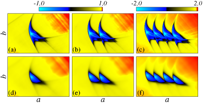
Figure 1: Enlargement of Hénon’s stable domains in two-dimensional parameter space ($a,b$) inside the interval $(a_{\mbox{\tiny min}},a_{\mbox{\tiny max}})=(1.713,1.743)$ and $(b_{\mbox{\tiny min}},b_{\mbox{\tiny max}})=(0.110,0.119)$ for noise intensities $7\times 10^{-5}$ (top row) and $2\times 10^{-4}$ (bottom row).

Being more specific, to motivate and exemplify our proposal, Fig. 1 displays the enlargement of stable domains in the two-dimensional parameter space ($a,b$) of the Hénon map $(x_{n+1},y_{n+1})=(1-ax_{n}^{2}+y_{n}+F_{n}+D\phi_{n},bx_{n})$ subjected to an external periodic force $F_{n}$ and a Gaussian noise $\phi_{n}$ with intensities proportional to $D=7\times 10^{-5}$ (top row) and $D=2\times 10^{-4}$ (bottom row). Blue colours are related to parameters which induce stable dynamics and yellow to red colours leading to chaotic dynamics. Plotted is the largest Lyapunov exponent (LE) (see colour bar). The stable domains are the SSs mentioned before but slightly deformed by noise Manchein et al. (2017); Horstmann et al. (2017). Going from Fig. 1(a) ($F=0$) to Fig. 1(b) ($F=8\times 10^{-4}$) and finally to Fig. 1(c) ($F=2\times 10^{-3}$), an astonishing increase of stable domains is observed. The increasing area of the stable domains are, when compared to Fig. 1(a), $85\%$ in Fig. 1(b) and $230\%$ in Fig. 1(c). The same behaviour is observed for the bottom row (same values of $F$) for which the gain is of $77\%$ for duplication [Fig. 1(e)] and $205\%$ for quadruplication [Fig. 1(f)] when compared to Fig. 1(d). The origin of such enlargement is that independent attractors are steered to distinct locations in phase space. Two attractors in Figs. 1(b) and (e) and four in Figs. 1(c) and (f). In this case the attractors are created and steered by the time dependent function $F_{n}$ which has period-2 ($+F,-F,+F,-F,\ldots$) in Fig. 1(b) and (e) and period-4 ($+F,-F/2,+F/4,-F,+F,-F/2,\ldots$) in Fig. 1(c) and (f). The physical and mathematical backgrounds of our findings are demonstrated next using realistic systems.  It is worth to mention here that in the above motivational example of the Hénon model, the multiattractors attractors are simultaneously created and moved in phase space. The Hénon map without external perturbation has only one attractor for the considered parameters.

This Letter shows that by steering multiple independent attractors in phase space, overlapped SSs split apart generating enlarged stable domains in parameter space, leading to a substantial enhanced resistance under parameter inaccuracy and noise. The replication of periodic windows in differential equations was previously reported in Medeiros et al. (2010, 2011), but a methodology to apply this procedure remained unclear. Our procedure introduces the concept of enhanced parameter flexibility under steering of attractors and should be applicable to all experiments and complex systems models whose underline dynamics presents multistability. Results are presented for two complete distinct physical situations, namely for the Ratchet current described by the Langevin equation and for the Chua’s circuit. While investigations about applications of ratchet effects are still very active Ding and et. al. (2018); Waitukaitis and et. al. (2017); Bramwell (2017); Brox and et. al. (2017); Erbas-Cakmal and et. al. (2017); Müller et al. (2017); Oliveira et al. (2016); Reichhardt and Reichhardt (2016); Budkin and Tarasenko (2016); Olbrich and et. al. (2016); Grossert et al. (2016); Bao-quan (2016), the Chua’s electronic circuit Chua (1992) contains all ingredients of regular and chaotic motion and is also of actual interest Talla and Woafo (2017); Stankevich et al. (2017); Shepelev et al. (2017); Peng and Min (2017).

Ratchet current in the Langevin equation. The most general way to describe unbiased currents in realistic systems is to integrate the Langevin equation with an asymmetric spatial potential, namely

$$\ddot{x}+\gamma\dot{x}-5.0[0.7\sin(2x)+\cos(x)]-K\sin(t)+\xi(t)=0,$$

where $x$ is the position, dot represents time derivative, $\xi(t)$ is the Gaussian thermal noise satisfying $\langle\xi(t)\rangle=0$ and obeying the dissipation-fluctuation relation $\langle\xi(t)^{2}\rangle=2\gamma K_{\mbox{\tiny B}}T\delta(t-t^{\prime})$. $K_{\mbox{\tiny B}}=1$ is the Boltzmann constant, $\gamma$ is the dissipation parameter which induces time irreversibility, $T$ the temperature and $K\sin(t)$ is the force which keeps physical states out of equilibrium. For distinct parameters combination ($K,\chi=e^{-\gamma}$), used to construct two-dimensional parameter spaces studied here, ratchet current may be generated, as shown in Fig. 2(a) for $T=0$. To integrate the Langevin equation we use fourth order Stochastic Runge-Kutta algorithm with fixed time-step $h=0.01$. Ratchet current is determined by double averages $\langle\langle\dot{x}\rangle\rangle$, one in time and the other one along $625$ equally distributed initial conditions (ICs) inside the interval $[-2\pi,2\pi]$, i.e. $\langle x(0)\rangle=\langle\dot{x}(0)\rangle=0$. Colours represent the values of the current, black for zero, green to blue for positive and yellow to red for negative currents. It is evident that for almost all parameter combination no ratchet current is observed. Exceptions are three regions with small currents (green points). Two of these regions, marked with cyan and yellow boxes contain SSs, not clearly visible due to the small current values. These SSs are more complicated SSs than those usually studied in the literature (see introduction). The thermal noise tends to destroy a considerable portion of the SSs, always starting from their antennas, decreasing the parameter combinations that generate non-zero ratchet current. This is displayed in Figs. 2(c) and (e) for $T=10^{-4}$.

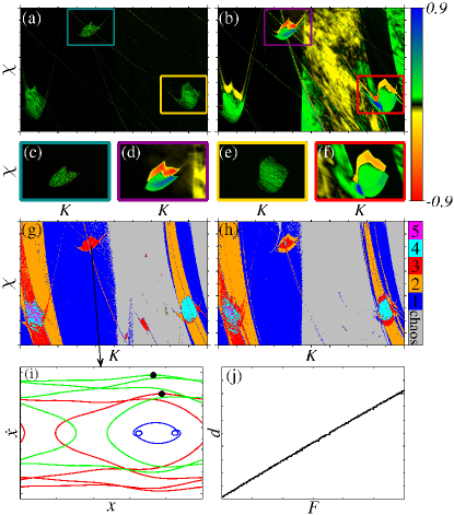
Figure 2: Two-dimensional parameter space $(K,\chi)$ for the Langevin equation plotting the ratchet current in (a) $F=0.0$ and (b) $F=0.3$, and the number of stable attractors in (g) for $F=0.0$ and (h) for $F=0.3$ using $(K_{\mbox{\tiny min}},K_{\mbox{\tiny max}})=(5.6,9.6)$ and $(\chi_{\mbox{\tiny min}},\chi_{\mbox{\tiny max}})=(0.7,0.9)$. Figures (c)-(f) show thermal effects using $T=10^{-4}$ for the regions selected by coloured boxes in (a) and (b). Figure (i) displays the stable attractors in phase-space $(x_{\mbox{\tiny min}},x_{\mbox{\tiny max}})=(-\pi,\pi)$ and $(\dot{x}_{\mbox{\tiny min}},\dot{x}_{\mbox{\tiny max}})=(-11,11)$, while (j) shows the distance $d$ between the black dots in (i), which are the maxima of velocity $\dot{x}$ for the attractors red and green,  in the ranges $(F_{\mbox{\tiny min}},F_{\mbox{\tiny max}})=(0.0,0.3)$ and $(d_{\mbox{\tiny min}},d_{\mbox{\tiny max}})=(3.4,3.5)$

In order to successfully apply our procedure we have to follow two fundamental steps. First is to check if the number of attractors for a parameter combination  of the unperturbed system is larger than one, i.e. if  there are multiattractors  in the correspondent phase space. This is displayed in Fig. 2(g) for the same two-dimensional parameter space from Fig. 2(a). In this case, colours are related to the number of periodic attractors, as shown in the colour bar. For each pair $(K,\chi)$ we calculated the time average $\langle\dot{x}\rangle$ for $25$ ICs equally distributed inside the interval $[-2\pi,2\pi]$ and, comparing them, it is possible to determine the number of different periodic attractors. Regions with chaotic attractors are easily found analysing the largest LE. It is well known that usually stable attractors generate efficient ratchet currents Celestino et al. (2011, 2013). Comparisons between Figs. 2(g) and (a) convince us that only regions with three and four stable attractors are able to generate the small currents. The blue and orange regions generate zero currents since attractors are located symmetrically around $\dot{x}=0$ (not shown). In order to explain the small currents in Fig. 2(a) we focus on the three stable attractors located inside the cyan box. Figure 2(i) displays these attractors located at $K=7.1$ and $\chi=0.865$. It is easy to see that the red and green attractors are not located completely symmetrically around $\dot{x}=0$, thus generating the small currents inside the cyan box from Fig. 2(a).

Now we come to the next step, which is to steer the stable attractors to distinct directions in phase and parameter spaces. This can be achieved by inserting in the above Langevin equation an additional external force

$$F(t)=F\cos(2t),$$

which has a distinct period and symmetry from the external oscillation force $K\sin(t)$ which is already there. Other kind of periodic forms for $F(t)$ could be used, depending on specifics needs, as discussed later. Figure 2(j) shows an example of how the distance $d$ between the maxima of $\dot{x}$ for two different attractors (see black dots in the attractors from Fig. 2(i)) changes as a function of $F$. In Fig. 2(h) the changes in the number of attractors in the two-dimensional parameter space can be observed for $F=0.3$. Attractors move in phase space and the SSs enlarge by a given amount. Not all of them move since this depends on the function $F(t)$, as mentioned above. Inside the periodic structures from the cyan box [compare Figs. 2(a),(g) and (h)] some regions remain with only two attractors from the three attractors shown in Fig. 2(i). The effect of such movements on the current is quite interesting and is plotted in Fig. 2(b) for $T=0.0$, and in Figs. 2(d) and (f) for $T=10^{-4}$. To see the efficiency of the procedure proposed here we have to compare Fig. 2(c) ($F=0$) with Fig. 2(d) ($F=0.3$) and Fig. 2(e) ($F=0$) with (f) ($F=0.3$). Figs. 2(d) and (f) display enlarged SSs and much larger values of the currents when compared to the cases with $F=0$. The increase of the regions with non-zero ratchet currents is around $85\%$ when comparing Fig. 2(a) and Fig. 2(b). From the total number of attractors found for a specific parameter combination $(K,\chi)$, two of them, with opposite value of $\langle\dot{x}\rangle$ (time average of $\dot{x}$), are steered leading to two independent SSs, which have opposite currents (blue and red). Thus, the available currents domains in parameter space are enlarged by moving apart the attractors in Fig. 2(i) with $\langle\dot{x}\rangle>0$ (green) and $\langle\dot{x}\rangle<0$ (red), avoiding the reduction of the total ratchet current when both attractors are found for same parameter combination $(K,\chi)$.

Chua’s electronic circuit. In this circuit the parameters are directly related to properties of the experimental device, namely, resistance, inductance and capacitances in the circuit. Due to experimental instabilities like electric voltage variations and noise, or even intrinsic imprecision in the resistance and capacitance values, there is no guarantee that the underline dynamics corresponds to the parameters for which the experiment was performed. According to the Kirchhoff’s laws applied for current and voltage in the circuit, we find the following first order differential equations:

$$\begin{array}[]{cl}&\dot{X}=\dfrac{dX}{dT}=\alpha\left[Y-X-I(X)\right],\\ \\ &\dot{Y}=\dfrac{dY}{dT}=X-Y+Z,\\ \\ &\dot{Z}=\dfrac{dZ}{dT}=-\beta Y-\gamma Z-\left(\dfrac{\beta}{B_{p}}\right)F(X)+\phi(t).\\ \end{array}$$ (1)

The piecewise linear current through the diode is $I(X)=bX+\frac{1}{2}(a-b)(|X+1|-|X-1|)$, with $a$ and $b$ being control parameters and $F(X)=K[\sin(B_{p}X)+A\cos(3B_{p}X)]$, which is the external asymmetric perturbation used to steer attractors. The adimensional states variables ($X,Y,Z$) are written in terms of the original states ($x,y,z$) as $X=x/B_{p},Y=y/B_{p}$ and $Z=zR/B_{p}$ and parameters $\alpha=C_{2}/C_{1}$, $\beta={R^{2}C_{2}}/{L}$, $\gamma={Rr_{L}C_{2}}/{L}$, $T={t}/{RC_{2}}$, and $I(X)=i_{d}(x)R/B_{p}$. The states ($x,y$) are the voltages across the capacitors $C_{1}$ and $C_{2}$ and $z$ the current across the inductor. $R$ and $L$ are passive linear elements and $r_{L}$ is the inductor-resistance. The fixed parameters are $a=-1.13996128$, $b=-0.7120006131$, $B_{p}=2.2$, $\beta=50.0$ and $K=0.01$, while $A$, $\alpha$ and $\gamma$ are varied. For $K=0$ the above system is the usual Chua’s circuit Chua (1992). For $A\neq 0$ the current asymmetry is introduced and leads to the steering of attractors. The effect of noise $\phi(t)$ is introduced in the $Z$ state variable and obeys a Gaussian distribution with $\langle\phi(t)\rangle=0$ and  $\langle\phi(t)^{2}\rangle=2D\delta(t-t^{\prime})$, being $D$ its intensity. Noise effects in the original Chua’s circuit is by itself an actual research subject Prebianca et al. (2018).

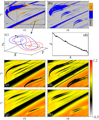
Figure 3: (Color online) Two-dimensional parameter spaces for Chua’s circuit showing the number of stable attractors in (a) $A=0.0$ and (b) $A=0.3$ for $(\alpha_{\mbox{\tiny min}},\alpha_{\mbox{\tiny max}})=(21.8,24.8)$ and $(\gamma_{\mbox{\tiny min}},\gamma_{\mbox{\tiny max}})=(-0.40,0.05)$. Panel (c) displays the two attractors found in the SS indicated by the black arrow in the phase space limited by $(X_{\mbox{\tiny min}},X_{\mbox{\tiny max}})=(-2.5,2.5)$, $(Y_{\mbox{\tiny min}},Y_{\mbox{\tiny max}})=(-0.4,0.4)$ and $(Z_{\mbox{\tiny min}},Z_{\mbox{\tiny max}})=(-5.0,5.0)$, while (d) shows the distance in coordinate $z$ between the black points as function of $A$  using $(A_{\mbox{\tiny min}},A_{\mbox{\tiny max}})=(0.0,0.15)$ and $(d_{\mbox{\tiny min}},d_{\mbox{\tiny max}})=(0.595,0.625)$. Figures (e)-(h) are magnifications of the black box displayed in (a) plotting the largest LE using (e) $A=0.0$, $D=0.0$, (f) $A=0.2$, $D=0.0$, (g) $A=0.0$, $D=10^{-5}$ and (g) $A=0.2$, $D=10^{-5}$.

As before, the first step in the procedure is to find the parameter combination for which there are more than one independent stable attractors in phase space. In this case, different stable attractors for a specific parameter combination $(\alpha,\gamma)$ are identified comparing the value of the lowest LE (related to the most stable direction) obtained for $64$ different ICs equally distributed in $(x_{\mbox{\tiny min}},x_{\mbox{\tiny max}})=(y_{\mbox{\tiny min}},y_{\mbox{\tiny max}})=(z_{\mbox{\tiny min}},z_{\mbox{\tiny max}})=(-0.2,0.2)$. This is shown in Fig. 3(a) in the two-dimensional parameter space ($\alpha,\gamma$) for the noiseless case and $A=0$. Blue for one, orange for two stable attractors and gray for chaotic attractors. For this system only regions with one and two attractors were found inside this parameter range. We call to attention that the structures of the stable regions are the shrimp-like SSs frequently found in the literature. Figure 3(c) shows exemplary two attractors in phase space for ($\alpha=24.06,\gamma=-0.31$) (see black arrow in Fig.3(a)). These attractors are obtained from distinct initial conditions and are therefore independent. Now we include the current asymmetry by using $A=0.3$ and the number of attractors for this case is displayed in Fig.3(b), demonstrating that only SSs with two attractors become separated. Each of the separated SSs have now only one stable attractor and the relative movement $d$ [distance between black points in Fig. 3(c)] of attractors as a function of $A$ is displayed in Fig. 3(d).

The next step is to measure the enlargement of SSs for $A\neq 0$ in the presence of noise. For clarity we analyse the enlargement inside the box shown in Fig. 3(a). Figure 3(e) for $A=0$ and Fig. 3(f) for $A=0.2$ compare the enlargement in parameter space obtained by steering the stable attractors for the noiseless case, while Figs. 3(g) and (h) compare the case with $D=10^{-5}$. Plotted in colours is the largest LE, black to white for stable motion and yellow to red for unstable motion. We observe that while the SSs with two attractors from Fig. 3(a) become enlarged, the central black stripe which has one attractor starts to be destroyed. This show the relevance to having SSs with more than one attractor. The increased area with stable dynamics in this case is around $60\%$ when comparing regions close to the duplicated SSs.

Discussion. The key procedure in the mechanism of steering multiattractors is to use  asymmetric time and/or space external forces capable of moving them independently in phase space.  A simple systematic scheme to apply our method is: (i) run the simulation/experiment for the desirable parameter combination in a regular regime, (ii) plot the stable attractor in phase space (or coexisting stable attractors, in case), (iii) insert an asymmetric (in time or/and in space) periodic external perturbation and (iv) run the simulation/experiment again, plot the attractor and compare it to the attractor found in item (ii) above. Check if the attractor is split in more attractors (in case the original attractor was degenerated) or if the coexisting attractors moved apart  or got closer. If yes, you achieved the needed extension of the available parameter which induce the same dynamics. If not, techniques to generated multiattractors in continuous systems Chizhevsky (2001) might be used. In this case, start again in step (i). In the crucial step (iii) there is a maximum of $D+1$ possibilities, where $D$ is the spatial dimension of the system. The method is very general (universal) since there is no need to know the symmetry of the attractors.  In addition, when the external force moves multiattractors equally in phase space, no enlargement of SSs is expected to occur. On the other hand, when such external forcing is chosen with appropriate parameters (amplitude and frequency) it may be used to suppress SSs in parameter space Mathias and Rech (2012), exactly the opposite of what is proposed here. We also have to mention a crucial difference between both continuous systems discussed here and the discrete Hénon map used in the motivation. While in the continuous cases the extra external force only steers the already existing multistable attractors, in the map it simultaneously creates and moves them in phase and parameter space, as demonstrated for one-dimensional da Silva et al. (2017) and two-dimensional Manchein et al. (2017) noiseless maps.

Conclusions. The steering of multistable attractors in phase space is proposed to enlarge the available parameters of physical devices which lead to a desired dynamics. This could be interpreted as a kind of chaos control Ott et al. (1990) in parameter space, but having the fundamental principle of moving multiattractors apart  or closer to each other. The enlarged stable domains (SSs) in parameter space,  only possible due to the existence of multiattractors, transform the underline dynamics more resistant to parameter inaccuracy and noise. Our procedure is motivated using the paradigmatic Hénon map with noise, and explained in details for the ratchet currents in a thermal bath and Chua’s electronic circuit with noise. The increasing percentage ($230\%$) of stable domains in Hénon’s map and regions with non-zero current ($85\%$) in the ratchet system are astonishing. In Chua’s electronic circuit the percentage gain is around $60\%$. While results for the Hénon map show the generality of our procedure in the context of discrete nonlinear systems, the ratchet current and Chua’s circuit represent realistic systems described by continuous differential equations under noise. Thus, our mechanism should be applicable to a wide range of physical systems whose underline dynamics presents multistability. In case the systems have just one attractor, hidden attractors may be found Stankevich et al. (2017); Cubero and Renzoni (2016) or multiattractors  might be created Chizhevsky (2001). Our proposal is also expected to be useful for experiments in distinct areas, ranging from electronic circuits, lasers, ratchet devices, Josephson junctions, population evolutions, fluid dynamics, neuronal models, among others. Besides the experimental demonstration of our findings, future investigations may analise steering effects of independent chaotic multiattractors.