Leaves on the line and in the plane

Abstract

The dead leaves model (DLM) provides a random tessellation of $d$-space, representing the visible portions of fallen leaves on the ground when $d=2$. For $d=1$, we establish formulae for the intensity, two-point correlations, and asymptotic covariances for the point process of cell boundaries, along with a functional CLT. For $d=2$ we establish analogous results for the random surface measure of cell boundaries, and also determine the intensity of cells in a more general setting than in earlier work of Cowan and Tsang. We introduce a general notion of dead leaves random measures and give formulae for means, asymptotic variances and functional CLTs for these measures; this has applications to various other quantities associated with the DLM.

Key words and phrases: random tessellation, dead leaves model, random measure, central limit theorem, Ornstein-Uhlenbeck process.

AMS classifications: 60D05, 60G57, 60G55, 60F05, 82C22.

1 Introduction

1.1 Overview

The dead leaves model (or DLM for short) in $d$-dimensional space ($d\in\mathbb{N}$), due originally to Matheron [21], is defined as follows [4, 34]. Leaves fall at random onto the ground and the visible parts of leaves on the ground (i.e., those parts that are not covered by later arriving leaves) tessellate $\mathbb{R}^{d}$ (typically with $d=2$; see Figure 1). Motivation for studying the DLM from the modelling of natural images, and from materials science, is discussed in [4], [15], and [8], for example. The DLM provides a natural way of generating a stationary random tessellation of the plane with non-convex cells having possibly curved boundaries.

To define the model more formally, let ${\mathbb{Q}}$ be a probability measure on the space ${\cal C}$ of compact sets in $\mathbb{R}^{d}$ (equipped with the $\sigma$-algebra generated by the Fell topology, as defined in Section 1.3 below), assigning strictly positive measure to the collection of sets in ${\cal C}$ having non-empty interior. A collection of ‘leaves’ arrives as an independently marked homogeneous Poisson point process ${\cal P}=\sum_{i=1}^{\infty}\delta_{(x_{i},t_{i})}$ in $\mathbb{R}^{d}\times\mathbb{R}$ of unit intensity with marks $(S_{i})_{i\geq 1}$ taking values in ${\cal C}$ with common mark distribution ${\mathbb{Q}}$. Each point $(x_{i},t_{i},S_{i})$ of this marked point process is said to have arrival time $t_{i}$ and the associated leaf covers the region $S_{i}+x_{i}\subset\mathbb{R}^{d}$ from that time onwards (where $S+x:=\{y+x:y\in S\}$). At a specified time, say time 0, and at spatial location $x\in\mathbb{R}^{d}$, the most recent leaf to arrive before time 0 that covers location $x$ is said to be visible (or exposed) at $x$. For each $i\in\mathbb{N}$, the visible portion of leaf $i$ at time 0 is the set of sites $x\in\mathbb{R}^{d}$ such that leaf $i$ is visible at $x$ at time 0. The connected components of visible portions of leaves (at time 0) form a tessellation of $\mathbb{R}^{d}$, which we call the DLM tessellation.

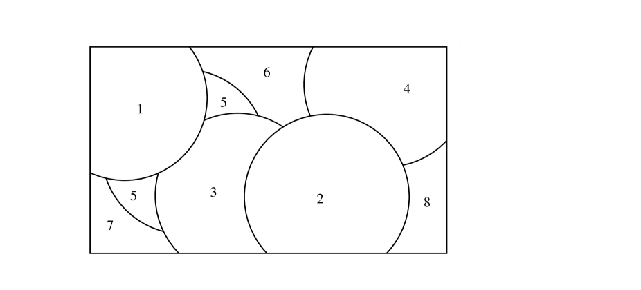
Figure 1: A realization of the DLM tessellation, restricted to a window, where all the leaves are unit disks. The numbers indicate the reverse order of arrival of the leaves visible within the window. In this paper we view the two visible components of leaf 5 as being separate components of the DLM tessellation

Properties of the DLM itself are discussed in [4, 6, 15, 34], while percolation on the DLM tessellation has been considered in [2, 24]. In some of these works the authors call the DLM the ‘confetti’ model. Note that in the present paper, all cells of our DLM tessellation are connected; the tessellation where cells are taken to be the visible portions of leaves (rather than their connected components) is also of interest, and is considered in some of the works just mentioned.

In this paper we consider the DLM for $d=1$ and for $d=2$. For $d=1$, we develop the second order theory for the point process of cell boundaries. That is, we determine its second factorial moment measure, two-point correlation functions, asymptotic variance and a spatial central limit theorem (CLT). Moreover, we can and do consider the point process to be evolving as leaves continue to rain down; we establish a functional CLT showing that the (evolving) number of cells in a large window approximates to an Ornstein-Uhlenbeck process. For $d=2$ we carry out a similar programme (asymptotic variance and functional CLT) for the surface measure of cell boundaries within a large window. We state our results for $d=1$ in Section 2, and for $d=2$ in Section 3.

For general $d$, we also develop (in Section 4) an extension of the DLM which we call the dead leaves random measure (DLRM). Suppose now that each point $(x_{i},t_{i})$ of ${\cal P}$ is marked with not only a random closed set $S_{i}$ as before, but also a random measure $M_{i}$, for example the surface measure of $\partial S_{i}$. The DLRM at time $t$ is the sum, over those $i$ with $t_{i}\leq t$, of the measures $M_{i}+x_{i}:=M_{i}(\cdot+(-x_{i}))$, restricted to the complement of leaves arriving between times $t_{i}$ and $t$. We give results on its intensity, limiting covariances and functional CLTs. This provides a general framework from which we may deduce the results already mentioned as special cases, and is also applicable to other DLM functionals and to variants of the DLM including the colour DLM and dead leaves random function, as discussed in Section 4.

As well as the new results already mentioned, we provide some extensions to known first-order results, giving the intensity of cell boundaries in $d=1$, and the intensity of cells in $d=2$. These were already in the literature in the special cases when all of the leaves are connected (for $d=1$; see [21]), and when they all have the same shape (for $d=2$; see [6]). Finally, for $d=1$ we discuss the distribution of cell sizes; essentially this was given in [21] but we give a bit more detail here.

Exact formulae for second moment measures and for two-point correlation functions are rarely available for non-trivial point processes in Euclidean space, and one contribution of this work is to provide such formulae in one class of such models. Our CLTs could be useful for providing confidence intervals for parameter estimation in the DLM and related models. Our general functional CLT shows that the DLRMs are a class of off-lattice interacting particle systems for which the limiting process of fluctuations can be identified explicitly as an Ornstein-Uhlenbeck process. In earlier works [28, 30], functional CLTs were obtained for certain general classes of particle systems but without any characterisation of the limit process.

The proof of some of our results in $d=2$ uses the following results. For rectifiable curves $\gamma$ and $\gamma^{\prime}$ in $\mathbb{R}^{2}$ of respective lengths $|\gamma|$ and $|\gamma^{\prime}|$, let $N(\gamma,\gamma^{\prime})$ (respectively ${\tilde{N}}(\gamma,\gamma^{\prime})$) denote the number of times they cross each other (respectively, touch each other). If one integrates $N(\gamma,T(\gamma^{\prime}))$ (resp. ${\tilde{N}}(\gamma,T(\gamma^{\prime}))$ over all rigid motions $T$ of the plane, one obtains a value of $4|\gamma|\times|\gamma^{\prime}|$ (resp. zero). We discuss these results, which are related to the classic Buffon’s needle problem, in Section 5.

Since we prefer to work with positive rather than negative times, in this paper we often consider a time-reversed version of the DLM where, for each site $x\in\mathbb{R}^{d}$, the first leaf to arrive at $x$ after time 0 is taken to be visible at $x$. Imagine leaves falling onto a glass plate which can be observed from below, starting from time 0. Clearly this gives a tessellation with the same distribution as the original DLM. This observation dates back at least to [12]. In [17], it is the basis for a perfect simulation algorithm for the DLM. The time-reversed DLM is illustrated for $d=1$ in Figure 2.

We shall state our results in Sections 2-5, and prove them in Sections 6-8.

Figure 2: A realization of the time-reversed DLM in $d=1$, with time as the vertical coordinate. The leaves are intervals of variable length. Those leaves arriving in a given rectangular region of space-time are shown, and the boundary points of the induced 1-dimensional DLM tessellation are shown at the bottom. The thicker lines represent leaves which are at least partially visible

1.2 Motivation

We now discuss further the motivation for considering the DLM. Since we consider the case $d=1$ in some detail, we discuss the motivation for this at some length.

The phrase ‘leaves on the line’ entered the British folklore in the early 1990s as a corporate justification for delays on the railways. To quote Wikipedia, this phrase is ‘a standing joke … seen by members of the public who do not understand the problem as an excuse for poor service.’ This paper is a mathematical contribution to said public understanding.

A one-dimensional DLM is obtained whenever one takes the restriction of a higher-dimensional DLM (in $\mathbb{R}^{d}$, say, with $d>1$) to a specified one-dimensional subspace of $\mathbb{R}^{d}$. Such restrictions are considered in [34] and [4].

Moreover, the one dimensional DLM is quite natural in its own right. For example, to quote [34], ‘Standing at the beginning of a forest, one sees only the first few trees, the others being hidden behind.’ A less pleasant interpretation, is that if an explosion takes place in a crowded spot, one might be interested in the number of people directly exposed to the blast (rather than shielded by others). In these two interpretations, the ‘time’ dimension in fact represents a second spatial dimension.

In another interpretation of the one-dimensional time-reversed DLM, consider a rolling news television or radio station. Suppose news stories arise as a homogeneous Poisson process in the product space $\mathbb{R}\times\mathbb{R}_{+}$, where the first coordinate represents the time at which the story starts, and the second coordinate represents its ‘newsworthiness’ (a lower score representing a more newsworthy story), and each story is active for a random duration. Suppose at any given time the news station presents the most newsworthy currently active story. Then the stories presented form a sequence of intervals, each story presented continuing until it finishes or is superseded by a more newsworthy story. The continuum time series of stories presented forms a DLM in time rather than in space, with ‘newsworthiness’ taking the role of ‘time’ in the original DLM. One can imagine a similar situation with, for example, the time series of top-ranked tennis or golf players.

In these interpretations, we are taking the trajectory of a news story’s newsworthiness, or a tennis player’s standard of play, to be flat but of possibly random duration. It would be interesting in future work to allow for other shapes of trajectory. If the trajectory is taken to be a fixed wedge-shape, then the sequence of top-ranked stories/players is the sequence of maximal points (actually minimal points in our formulation), which has been considered, for example, in [18, 37].

The two-dimensional DLM has received considerable attention in applications; see [4] and references therein. For any two-dimensional image of a three-dimensional particulate material with opaque particles, the closest particles obscure those lying behind, and the DLM models this phenomenon. See for example [15, 14] for applications to analysis of images of powders. Jeulin [13, 15] extends to the DLM to a dead leaves random function model for further flexibility in modelling greyscale images, and some of our results are applicable to this model. See Section 4.

Another reason to study the DLM, in arbitrary dimensions, is as an analogue to the car parking model of random sequential adsorption. In the one-dimensional and infinite-space version of the latter model, unit intervals (‘cars’) arrive at locations in space-time given by the points of a homogeneous Poisson process in $\mathbb{R}\times\mathbb{R}_{+}$. Each car is accepted if the position (a unit interval) where it arrives does not intersect any previously accepted cars. Ultimately, at time infinity one ends up with a random maximal (i.e., saturated) packing of $\mathbb{R}$ by unit intervals. The higher-dimensional version of the car parking model has also been studied, for example in [9] and references therein.

The problem of covering can be viewed as in some sense dual to that of packing (see for example [31, 39]), and in this sense the (time-reversed) DLM is dual to the car parking model; in each case, objects of finite but positive size (cars/leaves) arrive sequentially at random in $d$-space, and are accepted in a greedy manner subject to a hard-core constraint (for the packing) or a visibility constraint (for the DLM).

1.3 Notation and terminology

Let ${\cal B}^{d}$ denote the Borel $\sigma$-algebra on $\mathbb{R}^{d}$. For $k\in\{0,1,\ldots,d\}$, let ${\cal H}_{k}$ denote the $k$-dimensional Hausdorff measure of sets in $\mathbb{R}^{d}$. This is a measure on $(\mathbb{R}^{d},{\cal B}^{d})$. In particular, ${\cal H}_{0}$ is the counting measure and ${\cal H}_{d}$ is Lebesgue measure. See [19].

Let $\|\cdot\|$ denote the Euclidean norm in $\mathbb{R}^{d}$. Given $x\in\mathbb{R}^{d}$, let $\delta_{x}$ denote the Dirac measure at $x$, i.e. $\delta_{x}(A)=1$ if $x\in A$, otherwise $\delta_{x}(A)=0$. For $r>0$, let $B(r):=\{y\in\mathbb{R}^{d}:\|y\|\leq r\}$, the closed Euclidean ball of radius $r$ centred on the origin. Set $\pi_{d}:={\cal H}_{d}(B(1))$, the Lebesgue measure of the unit ball in $d$ dimensions.

We say a set $\gamma\subset\mathbb{R}^{2}$ is a rectifiable curve if there exists a continuous injective function $\Gamma:[0,1]\to\mathbb{R}^{2}$ such that $\gamma=\Gamma([0,1])$ and ${\cal H}_{1}(\gamma)<\infty$. If moreover there exist $k\in\mathbb{N}\cup\{0\}$ and numbers $0=x_{0}<x_{1}<\cdots<x_{k+1}=1$, such that for $1\leq i\leq k+1$ the restriction of $\Gamma$ to $[x_{i-1},x_{i}]$ is continuously differentiable with derivative that is nowhere zero, we say that $\gamma$ is a piecewise $C^{1}$ curve. We then refer to the points $\Gamma(x_{1}),\ldots,\Gamma(x_{k})$ (where $k$ is assumed to be taken as small as possible) as the corners of $\gamma$. If we can take $k=0$ (so there are no corners), then we say $\gamma$ is a $C^{1}$ curve. We say that $\Gamma(0)$ and $\Gamma(1)$ are the endpoints of $\gamma$. We define a rectifiable Jordan curve (respectively, a piecewise $C^{1}$ Jordan curve) similarly to a rectifiable curve (respectively, piecewise $C^{1}$ curve) except that now $\Gamma$ must satisfy $\Gamma(1)=\Gamma(0)$ but be otherwise injective.

For $\sigma\geq 0$, let ${\cal N}(0,\sigma^{2})$ denote a normally distributed random variable having mean zero and variance $\sigma^{2}$ if $\sigma>0$, and denote a random variable taking the value 0 almost surely if $\sigma=0$.

We now review some concepts from the theory of point processes and random measures that we shall be using. See for example [19] or [33] for more details.

Let ${\bf M}$ be the space of locally finite measures on $(\mathbb{R}^{d},{\cal B}^{d})$, equipped with the smallest $\sigma$-algebra that makes measurable all of the functions from ${\bf M}$ to $\mathbb{R}$ of the form $\mu\mapsto\mu(A)$, with $A\in{\cal B}^{d}$. For $\mu\in{\bf M}$ we shall often write $|\mu|$ for $\mu(\mathbb{R}^{d})$. A random measure on $\mathbb{R}^{d}$ is a measurable function from an underlying probability space to ${\bf M}$, or equivalently, a measurable kernel from the probability space to $(\mathbb{R}^{d},{\cal B}^{d})$. A random measure on $\mathbb{R}^{d}$ is said to be stationary if its distribution is shift invariant, in which case the expected value of the measure it assigns to a Borel set $B\subset\mathbb{R}^{d}$ is proportional to the Lebesgue measure of $B$; the constant of proportionality is called the intensity of the random measure.

A random measure on $\mathbb{R}^{d}$ taking integer values is called a point process on $\mathbb{R}^{d}$, and the notions of intensity and stationarity for random measures carry through to point processes. A point process is said to be simple if it has no multiple points.

The second factorial moment measure of a point process $\eta$ in $\mathbb{R}^{d}$ is a Borel measure $\alpha_{2}$ on $\mathbb{R}^{d}\times\mathbb{R}^{d}$, defined at [19, eqn (4.22)]. For disjoint Borel sets $A,B\subset\mathbb{R}^{d}$, we have $\alpha_{2}(A\times B)=\mathbb{E}\,[\eta(A)\eta(B)].$ If $\eta$ is simple then for $x,y\in\mathbb{R}^{d}$ with $x\neq y$, loosely speaking $\alpha_{2}(d(x,y))$ is the probability of seeing a point of $\eta$ in $dx$ and another one in $dy$. If $\alpha_{2}(d(x,y))=\rho(y-x)dxdy$ for some Borel function $\rho:\mathbb{R}^{d}\to\mathbb{R}_{+}$, then the pair correlation function $\rho_{2}(\cdot)$ of the point process $\eta$ is defined by $\rho_{2}(z):=\rho(z)/\gamma^{2}$, where $\gamma$ is the intensity of $\eta$.

The Fell topology on ${\cal C}$ is the topology generated by all sets of the form $\{F\in{\cal C}:F\cap G\neq\varnothing\}$ with $G\subset\mathbb{R}^{d}$ open, or of the form $\{F\in{\cal C}:F\cap K=\varnothing\}$ with $K\in{\cal C}$.

A random closed set in $\mathbb{R}^{d}$ is a measurable map from a probability space to the space of closed sets in $\mathbb{R}^{d}$ equipped with the sigma-algebra generated by the Fell topology. See [33, Definition 2.1.2] or [23, Definition 1.1.$1^{\prime\prime}$]. A simple point process on $\mathbb{R}^{d}$ can also be interpreted as a random, locally finite set of points in $\mathbb{R}^{d}$.

We now elaborate on the definition of the DLM given already. Let ${\mathbb{Q}}$ be a probability measure on ${\cal C}$, which we call the grain distribution of the model. Assume ${\mathbb{Q}}$ assigns strictly positive measure to the collection of sets in ${\cal C}$ having non-empty interior. Let ${\cal P}$ be a homogeneous Poisson process in $\mathbb{R}^{d}\times\mathbb{R}$ of unit intensity. Write ${\cal P}=\sum_{i=1}^{\infty}\delta_{(x_{i},t_{i})}$ with $(x_{i},t_{i})_{i\in\mathbb{N}}$ a sequence of random elements of $\mathbb{R}^{d}\times\mathbb{R}$. This can be done: see [19, Corollary 6.5]. Independently of ${\cal P}$, let $(S_{i})_{i\geq 1}$ be a sequence of independent random elements of ${\cal C}$ with common distribution ${\mathbb{Q}}$. By the Marking theorem (see (see [19, Theorem 5.6]) the point process $\sum_{i=1}^{\infty}\delta_{(x_{i},t_{i},S_{i})}$ is a Poisson process in $\mathbb{R}^{d}\times\mathbb{R}\times{\cal C}$ with intensity measure ${\cal H}_{d}\otimes{\cal H}_{1}\otimes{\mathbb{Q}}$.

For $A\subset\mathbb{R}^{d}$, let $\overline{A}$ denote its closure and $A^{o}$ its interior; let $\partial A:=\overline{A}\setminus A^{o}$, the topological boundary of $A$. The boundary of the DLM tessellation at time $t$, which we denote by $\Phi_{t}$, is given by

$$\Phi_{t}:=\cup_{i:t_{i}\leq t}[(\partial S_{i}+x_{i})\setminus\cup_{j:t_{i}<t_{j}\leq t}(S_{j}^{o}+x_{j})].$$ (1.1)

The boundary of the the time-reversed DLM tessellation is denoted by $\Phi$, and given by

$$\Phi:=\cup_{i:t_{i}\geq 0}[(\partial S_{i}+x_{i})\setminus\cup_{j:0\leq t_{j}<t_{i}}(S_{j}^{o}+x_{j})].$$ (1.2)

The cells of our (time-reversed) DLM tessellation are then defined to be the closures of the connected components of $\mathbb{R}^{d}\setminus\Phi$. Clearly $\Phi_{t}$ has the same distribution as $\Phi$ for all $t$.

Throughout, we let $S$ denote a random element of ${\cal C}$ with distribution ${\mathbb{Q}}$; that is, a measurable function from an underlying probability space (denoted $(\Omega,{\cal F},{\mathbb{P}})$) to ${\cal C}$. For $x\in\mathbb{R}^{d}$ we set

$$\lambda:=\mathbb{E}\,[{\cal H}_{d}(S)];~{}~{}~{}~{}~{}~{}~{}\lambda_{x}:=\mathbb{E}\,[{\cal H}_{d}(S\cup(S+x))].$$ (1.3)

Clearly $0<\lambda\leq\lambda_{x}\leq 2\lambda$. We set

$$R:=\sup\{\|x\|:x\in S\},$$ (1.4)

taking $R=0$ if $S$ is empty. Observe that $2\lambda-\lambda_{x}$ equals the expected value of ${\cal H}_{d}(S\cap(S+x))$, sometimes called the covariogram of $S$. The function $\lambda_{x}$ will feature in certain formulae for limiting covariances below. It also features in certain formulae for limiting variances arising from the Boolean model (see for example [10]). The Boolean model, that is the random set $\cup_{i:0\leq t_{i}\leq\lambda}(S_{i}+x_{i})$ for some fixed $\lambda$, is another fundamental model in stochastic geometry.

Some of our results require the following measurability condition.

Condition 1.1.

${\mathbb{Q}}$ is such that ${\cal H}_{d-1}(\cdot\cap\partial S)$ is a random measure on $\mathbb{R}^{d}$.

For $d=1$, we shall show in Lemma 6.2 that Condition 1.1 can actually be deduced from our earlier assumption that $S$ is a random element of ${\cal C}$, that is, a measurable map from a probability space to ${\cal C}$. However, we do not know whether this is also the case for $d\geq 2$.

Given $d$, for $n>0$ let $W_{n}:=[0,n^{1/d}]^{d}$, a cube of volume $n$ in $d$-space. Let ${\cal R}_{0}$ denote the class of bounded measurable real-valued functions on $\mathbb{R}^{d}$ that are Lebesgue-almost everywhere continuous and have compact support (the ${\cal R}$ stands for ‘Riemann integrable’). For $f\in{\cal R}_{0}$, and $n>0$, define the rescaled function $T_{n}f$ by $T_{n}f(x):=f(n^{-1/d}x)$, for $x\in\mathbb{R}^{d}$. Given a measure $\mu$ on $\mathbb{R}^{d}$ we shall often write $\mu(f)$ for $\int_{\mathbb{R}^{d}}fd\mu$. Also, we write $\|f\|_{2}$ for $(\int_{\mathbb{R}^{d}}|f(x)|^{2}dx)^{1/2}$, and for $f,g\in{\cal R}_{0}$ we write $\langle f,g\rangle$ for $\int_{\mathbb{R}^{d}}f(x)g(x)dx$.

For $A,B\subset\mathbb{R}^{d}$ we set $A\oplus B:=\{a+b:a\in A,b\in B\}$.

2 Leaves on the line

In this section we take $d=1$ and state our results for the $1$-dimensional DLM. We shall prove them in Section 7.

We define a visible interval to be a cell of the DLM tessellation. In the special case where all of the leaves are single intervals of fixed length, a visible interval is simply the visible part of a leaf, because this visible part cannot be disconnected.

The endpoints of the visible intervals form a stationary point process in $\mathbb{R}$. In terms of earlier notation this point process is simply the random set $\Phi$ (if viewed as a random subset of $\mathbb{R}$) or the measure ${\cal H}_{0}(\Phi\cap\cdot)$ (if viewed as a random point measure). We denote this point process (viewed as a random measure) by $\eta$, as illustrated in Figure 2. The point process $\eta$ is simple, even if some of the leaves include constituent intervals of length zero (recall that we assume ${\mathbb{Q}}$ is such that some of the leaves have non-empty interior).

Our main results for $d=1$ concern the second factorial moment measure and the pair correlation function of $\eta$ (Theorem 2.2), asymptotic covariances and a CLT for the total number of points of $\eta$ in a large interval (Theorems 2.3, 2.4, and 2.5), and a functional CLT for this quantity as the DLM evolves in time (Theorem 2.6).

We shall also give formulae for the intensity of $\eta$, the distribution of the length of the visible interval containing the origin and the length of a typical visible interval (Propositions 2.1, 2.7 and 2.8). These propositions are to some extent already known, as we shall discuss.

Recall that $\lambda$ and $R$ are defined by (1.3) and (1.4), respectively.

Proposition 2.1 (Intensity of $\eta$).

Assume that $\mathbb{E}\,[R]<\infty$ and $\mathbb{E}\,[{\cal H}_{0}(\partial S)]<\infty$. Then $\eta$ is a stationary point process with intensity ${\lambda}^{-1}\mathbb{E}\,[{\cal H}_{0}(\partial S)]$.

Remarks. In the special case where all the leaves are intervals of strictly positive length, the intensity of $\eta$ simplifies to just $2/\lambda$. This special case of Proposition 2.1 is already documented; see [21, page 4], or [34, (XIII.41)].

Our more general statement (and proof) of Proposition 2.1 allows for disconnected leaves. If ${\cal H}_{0}(\partial S)$ is finite, then $S$ consists of finitely many disjoint intervals, and ${\cal H}_{0}(\partial S)$ equals twice the number of constituent intervals of $S$, minus the number of these intervals having length zero. It is quite natural to allow a leaf to have several components; for example if the one-dimensional DLM is obtained as the restriction of a higher-dimensional DLM (in $\mathbb{R}^{d}$, say, for some $d>1$) to a specified one-dimensional subspace of $\mathbb{R}^{d}$. If the leaves in the parent DLM in $\mathbb{R}^{d}$ are not restricted to be convex, but have ‘nice’ boundaries (for example the polygonal boundaries considered in [6]), then the one-dimensional DLM induced in this manner will typically include leaves with more than one component. The proof given here, based on a general result for DLRMs, and ultimately on the Mecke formula from the theory of Poisson processes [19], is quite simple and may be new.

In the next two results we use the following notation. Let $\nu$ denote the distribution of the Lebesgue measure of a leaf under the measure ${\mathbb{Q}}$. Let $H$ denote a random variable with distribution $\nu$. For $x>0$, write $F(x)=\mathbb{P}[H\leq x]$ and ${\overline{F}}(x):=1-F(x)$, and set $\lambda_{x}:=\mathbb{E}\,[H+\min(x,H)]$ (this is consistent with (1.3)).

Theorem 2.2 (Second moment measure of $\eta$).

Suppose that ${\mathbb{Q}}$ is concentrated on connected sets (i.e., on intervals), and that $F(0)=0$ and $\lambda<\infty$. Then the second factorial moment measure $\alpha_{2}$ of the point process $\eta$ is given for $x<y$ by

$$\alpha_{2}(d(x,y))=4(1+F(y-x))(\lambda\lambda_{y-x})^{-1}dydx+{\lambda}_{y-x}^{-1}\mathbb{P}[H+x\in dy]dx.$$ (2.1)

If $\nu$ has a probability density function $f$, then the pair correlation function $\rho_{2}$ of $\eta$ is given by

$$\rho_{2}(z)=\frac{\lambda(1+F(z))}{\lambda_{z}}+\frac{\lambda^{2}f(z)}{4\lambda_{z}},~{}~{}~{}z>0.$$ (2.2)

In the particular case where $\nu=\delta_{\lambda}$ for some $\lambda>0$, we have for $x<y$ that

$$\alpha_{2}(d(x,y))=\frac{4{\bf 1}_{(0,{\lambda})}(y-x)}{\lambda({\lambda}+y-x)}dydx+8{\lambda}^{-2}{\bf 1}_{({\lambda},\infty)}(y-x)dydx+(2{\lambda})^{-1}\delta_{{\lambda}+x}(dy)dx.$$

(2.3)

We now give some limit theorems for $\eta([0,n])$, as $n\to\infty$. In these results, $n$ does not need to be integer-valued.

Theorem 2.3 (Asymptotic variance for $\eta([0,n])$).

Suppose that $\mathbb{E}\,[({\cal H}_{0}(\partial S))^{2}]<\infty$ and $\mathbb{E}\,[R^{2}]<\infty$. Then the limit $\sigma_{1}^{2}:=\lim_{n\to\infty}n^{-1}{\rm Var}[\eta([0,n])]$ exists. If also ${\mathbb{Q}}$ is concentrated on intervals, and $F(0)=0$, then

$$\sigma_{1}^{2}=\frac{2}{{\lambda}}+2\int_{(0,\infty)}\lambda_{u}^{-1}\mathbb{P}[H\in du]+8\int_{0}^{\infty}\left(\frac{1+F(u)}{{\lambda}{\lambda}_{u}}-\frac{1}{{\lambda}^{2}}\right)du.$$ (2.4)

In (2.4) the last integrand on the right hand side is equal to

$$\frac{\int_{u}^{\infty}{\overline{F}}(t)dt-{\lambda}{\overline{F}}(u)}{{\lambda}^{2}(2{\lambda}-\int_{u}^{\infty}{\overline{F}}(t)dt)}.$$ (2.5)

In the special case with $\nu=\delta_{1}$, the right hand side of (2.4) comes to $8\log 2-5\approx 0.545$

It is interesting to consider the evolving point process of visible leaf boundaries. For $t\in\mathbb{R}$ let $\eta_{t}:={\cal H}_{0}(\Phi_{t}\cap\cdot)$, the point process of endpoints of visible intervals at time $t$, for the DLM run forward in time. See Figure 3. We use the abbreviation $\eta_{t}(n)$ for $\eta_{t}([0,n])$.

Theorem 2.4 (Asymptotic covariance for $\eta_{t}(n)$).

Suppose that $\mathbb{E}\,[({\cal H}_{0}(\partial S))^{2}]<\infty$ and $\mathbb{E}\,[R^{2}]<\infty$. Let $t,u\in\mathbb{R}$ and $r,s\in\mathbb{R}_{+}:=[0,\infty)$. Then with $\sigma_{1}^{2}$ as given in the preceding theorem,

$$\lim_{n\to\infty}n^{-1}{\rm Cov}(\eta_{t}(nr),\eta_{u}(ns))=\sigma_{1}^{2}(\min(r,s))\exp(-\lambda(|u-t|))$$

$$=:\kappa_{1}((r,t),(s,u)).$$ (2.6)

Figure 3: Illustration of the evolving DLM tessellation in $d=1$ with the point processes $\eta_{t}$ and $\eta_{u}$ shown. Here $t<u$.

Theorem 2.5 (CLT for $\eta_{t}(n)$).

Suppose that there exist constants $\varepsilon,K\in(0,\infty)$ such that $\mathbb{E}\,[({\cal H}_{0}(\partial S))^{2+\varepsilon}]<\infty$ and $\mathbb{P}[R\leq K]=1$. Then as $n\to\infty$,

$$n^{-1/2}(\eta([0,n])-\mathbb{E}\,\eta([0,n]))\stackrel{{\scriptstyle{\cal D}}}{{\longrightarrow}}{\cal N}(0,\sigma^{2}_{1}),$$ (2.7)

where $\sigma^{2}_{1}$ is given in Theorem 2.3. More generally, the finite-dimensional distributions of the random field $(n^{-1/2}(\eta_{t}(ns)-\mathbb{E}\,[\eta_{t}(ns)]),(s,t)\in\mathbb{R}_{+}\times\mathbb{R})$ converge to those of a centred Gaussian random field with covariance function $\kappa_{1}((r,t),(s,u))$ as defined in (2.6).

By the case $s=1$ of Theorem 2.5, the finite dimensional distributions of the process $(n^{-1/2}(\eta_{t}(n)-\mathbb{E}\,[\eta_{t}(n)]),t\in\mathbb{R})$ converge to those of a Gaussian process $(X_{t})_{t\in\mathbb{R}}$ with covariance function $\sigma_{1}^{2}\exp(-\lambda|u-t|)$. This limiting process is a stationary Ornstein-Uhlenbeck process; see [16, page 358]. That is, it is the solution to the stochastic differential equation

$$dX_{t}=-\lambda X_{t}dt+(2\lambda)^{1/2}\sigma_{1}dB_{t},$$

where $(B_{t})$ is a standard Brownian motion. Under a stronger moment condition, we can improve this finite dimensional convergence to a functional CLT; that is, to convergence in $D(-\infty,\infty)$ of right-continuous functions on $\mathbb{R}$ with left limits. We give this space the Skorohod topology, as described in [3] and extended to non-compact time intervals in [36].

Theorem 2.6 (Functional CLT for $\eta_{t}(n)$).

Suppose there exist $\varepsilon,K\in(0,\infty)$ such that $\mathbb{E}\,[({\cal H}_{0}(\partial S))^{4+\varepsilon}]<\infty$ and $\mathbb{P}[R\leq K]=1$. Then as $n\to\infty$, the stochastic process $(n^{-1/2}(\eta_{t}(n)-\mathbb{E}\,[\eta_{t}(n)]),t\in\mathbb{R})$ converges in distribution, in the space $D(-\infty,\infty)$, to the stationary Ornstein-Uhlenbeck Gaussian process with covariance function $\sigma_{1}^{2}\exp(-\lambda|u-t|),$ $t,u\in\mathbb{R}$.

The limiting random field in Theorem 2.5 is an Ornstein-Uhlenbeck process in Wiener space. See for example [26] for a definition, or [22] for a more detailed discussion of this infinite-dimensional Ornstein-Uhlenbeck process. It would be interesting, in future work, to try to extend the finite dimensional convergence of Theorem 2.5 to convergence in an appropriate two-parameter function space. This is beyond the scope of the methods used here, since our proof is based ultimately on the classical approach of [3] for showing convergence of a sequence of processes with a single time parameter, namely finite-dimensional convergence plus tightness via moment bounds.

It would also be of interest to extend these CLTs to cases where the leaves are intervals of unbounded length but satisfy a moment condition.

We conclude this section with results on the length of the interval of the DLM tessellation containing the origin, and the length of a ‘typical interval’. These follow from results in [21], as we discuss in Section 7. For an alternative proof, see the earlier version [29] of the present paper.

Proposition 2.7 (Exposed interval length distribution).

Assume that ${\mathbb{Q}}$ is concentrated on intervals of strictly positive length, and that $\lambda<\infty$. Let $\nu$ denote the distribution of the length of a leaf under the measure ${\mathbb{Q}}$, and $X$ the length of the visible interval covering the origin. The distribution of $X$ is given by

$$\mathbb{P}[X\in dx]=\left(\int_{(x,\infty)}\left(\frac{2x({\lambda}+u)}{({\lambda}+x)^{3}}\right)\nu(du)\right)dx+\frac{x\nu(dx)}{x+{\lambda}}.$$ (2.8)

In the special case where the measure $\nu$ is the Dirac measure $\delta_{\lambda}$ for some ${\lambda}>0$,

$$\mathbb{P}[X\in dx]=\left(\frac{4{\lambda}x}{({\lambda}+x)^{3}}\right){\bf 1}_{\{x<{\lambda}\}}dx+(1/2)\delta_{{\lambda}}(dx).$$ (2.9)

If $\nu$ is a Dirac measure, then $X$ is the length of the visible part of the leaf visible at the origin. In general, $X$ counts the length only of the connected component of the visible part of this leaf that includes $0$, ignoring any other components.

A typical visible interval, loosely speaking, is obtained by fixing a very large region of $\mathbb{R}$, and choosing at random one of the inter-point intervals of $\eta$ that lie in that region. The distribution of the length of a typical visible interval is the inverse-size-biased distribution of $X$ (see [19, Proposition 9.7]); that is, if $Y$ is the length of a typical visible interval we have $\mathbb{P}[Y\in dy]=y^{-1}\mathbb{P}[X\in dy]/\mathbb{E}\,[X^{-1}]$. Now $\mathbb{E}\,[X^{-1}]=2/\lambda$, which can be deduced either from (2.8) or from Proposition 2.1 using [19, eqn (9.22)]. Hence from (2.8) we have the following.

Proposition 2.8.

Let $Y$ denote the length of a typical visible interval. Under the assumptions of Proposition 2.7, the distribution of $Y$ is given by

$$\mathbb{P}[Y\in dy]=\left(\int_{(y,\infty)}\left(\frac{{\lambda}({\lambda}+u)}{({\lambda}+y)^{3}}\right)\nu(du)\right)dy+\frac{{\lambda}\nu(dy)}{2(y+{\lambda})}.$$ (2.10)

If all the leaves are intervals of length $\lambda$, i.e. $\nu=\delta_{\lambda}$ for some $\lambda>0$, then $Y$ has a mixed distribution with

$$\mathbb{P}[Y\in dy]=\left(\frac{2\lambda^{2}{\bf 1}_{(0,\lambda)}(y)}{(\lambda+y)^{3}}\right)dy+(1/4)\delta_{\lambda}(dy).$$

3 Leaves in the plane

In this section we take $d=2$, and state our results for the two-dimensional DLM. We shall prove them in Section 8.

We shall say that our grain distribution ${\mathbb{Q}}$ has the rectifiable Jordan property if it is concentrated on nonempty regular compact sets having a rectifiable Jordan curve as their boundary. Here, we say a compact set in $\mathbb{R}^{2}$ is regular if it is the closure of its interior. We say ${\mathbb{Q}}$ has the piecewise $C^{1}$ Jordan property if it is concentrated on sets having a piecewise $C^{1}$ Jordan curve as their boundary.

Recalling the definitions (1.1) and (1.2), define the measures $\phi:={\cal H}_{1}(\Phi\cap\cdot)$, the restriction of the one-dimensional Hausdorff measure to the boundaries of the DLM tessellation, and $\phi_{t}:={\cal H}_{1}(\Phi_{t}\cap\cdot)$ for $t\in\mathbb{R}$. As in (1.3), we set $\lambda:=\mathbb{E}\,[{\cal H}_{2}(S)]$, and $\lambda_{x}:=\mathbb{E}\,[{\cal H}_{2}(S\cup(S+x))]$ for $x\in\mathbb{R}^{2}$, where $S$ is a random element of ${\cal C}$ with distribution ${\mathbb{Q}}$ as per usual. Define $R$ by (1.4).

Theorem 3.1 (Intensity of cell boundaries).

Suppose that Condition 1.1 holds and $\mathbb{E}\,[{\cal H}_{2}(S\oplus B(1))]<\infty$. Then $\phi$ is a stationary random measure and its intensity is $\lambda^{-1}\mathbb{E}\,[{\cal H}_{1}(\partial S)].$

As mentioned earlier, the cells of the (time-reversed) DLM tessellation are the closures of the connected components of the set $\mathbb{R}^{2}\setminus\Phi$. We now define $\Xi$ to be the set of points in $\mathbb{R}^{2}$ which lie in three or more cells of this tessellation. Later we shall view $\Phi$ as a planar graph with the points of $\Xi$ as the nodes, which we call branch points, in this graph. We define the measure $\chi:={\cal H}_{0}(\Xi\cap\cdot)$.

For $A\subset\mathbb{R}^{2}$ and $\theta\in(-\pi,\pi]$, let $\rho_{\theta}(A)$ denote the image of $A$ under an anticlockwise rotation through an angle $\theta$ about the origin (elsewhere we are using $\rho_{2}$ to denote pair correlation, but this clash of notation should not be confusing). We say ${\mathbb{Q}}$ is rotation invariant if $\rho_{\theta}(S)\stackrel{{\scriptstyle{\cal D}}}{{=}}S$ for all $\theta\in(-\pi,\pi]$.

Theorem 3.2 (Intensity of branch points).

Assume either that ${\mathbb{Q}}$ has the piecewise $C^{1}$ Jordan property, or that ${\mathbb{Q}}$ has the rectifiable Jordan property and is rotation invariant. Assume also that $\lambda<\infty$, and $\mathbb{E}\,[R^{2}]<\infty$, and set

$$\beta_{3}:=\lambda^{-2}\int_{{\cal C}}\int_{{\cal C}}\int_{\mathbb{R}^{2}}{\cal H}_{0}(\partial\sigma\cap(\partial\sigma^{\prime}+x))dx{\mathbb{Q}}(d\sigma){\mathbb{Q}}(d\sigma^{\prime}).$$ (3.1)

Then: (a) If $\beta_{3}<\infty$, then $\chi$ is a stationary point process, with intensity $\beta_{3}$.

(b) If ${\mathbb{Q}}$ is rotation invariant, then

$$\beta_{3}=\frac{2}{\pi\lambda^{2}}\left(\mathbb{E}\,[{\cal H}_{1}(\partial S)]\right)^{2}.$$ (3.2)

The next two results require ${\mathbb{Q}}$ to have a further property. We say ${\mathbb{Q}}$ has the non-containment property if for $({\mathbb{Q}}\otimes{\mathbb{Q}})$-almost all pairs $(\sigma,\sigma^{\prime})\in{\cal C}\times{\cal C}$, the set of $x\in\mathbb{R}^{2}$ such that $\sigma+x\subset\sigma^{\prime}$ is Lebesgue-null. One way to guarantee the non-containment property is to have ${\mathbb{Q}}$ be such that under ${\mathbb{Q}}$, all of the sets $S_{i}$ have the same area.

Theorem 3.3 (Connectivity of $\Phi$).

Suppose ${\mathbb{Q}}$ has the rectifiable Jordan and non-containment properties, and that $\mathbb{E}\,[R^{2}]<\infty$. Then $\Phi$ is almost surely a connected set.

Let $\Psi$ be the set of centroids of cells of the DLM tessellation, and define the measure $\psi:={\cal H}_{0}(\Psi\cap\cdot)$. While we would expect that $\psi$ is a point process (i.e., that it is measurable), we have not proved this in general (unlike in the case of $\chi$), so we leave this as an open problem and include the measurability as an assumption in the next result.

Theorem 3.4 (Intensity of cells).

Suppose ${\mathbb{Q}}$ has the rectifiable Jordan and non-containment properties, and either has the piecewise $C^{1}$ Jordan property or is rotation invariant. Assume that $\beta_{3}<\infty$, and $\mathbb{E}\,[R^{2}]<\infty$, and that $\psi$ is a point process. Then $\psi$ is a stationary point process, and its intensity, denoted $\beta_{1}$, is given by $\beta_{1}=\beta_{3}/2$. In particular, if ${\mathbb{Q}}$ is rotation invariant, then

$$\beta_{1}=(\pi\lambda^{2})^{-1}(\mathbb{E}\,[{\cal H}_{1}(\partial S)])^{2}.$$ (3.3)

Remarks. Our formula for the intensity of $\phi$ in Theorem 3.1 agrees with that of [6, p. 57] but is considerably more general. In [6] it is assumed that ${\mathbb{Q}}$ is such that a random set $S$ with distribution ${\mathbb{Q}}$ is a uniform random rotation of a fixed polygon $S_{0}$. In [6, Sec. 7] there is some discussion on generalising to the case where $S_{0}$ is non-polygonal, but it is still taken to be a fixed set. Similarly, Equations (3.2) and (3.3) also generalize formulae in [6].

Theorem 3.3 is perhaps intuitively obvious, but a careful proof seems to require some effort. As well as being of interest in itself, the connectivity of $\Phi$ is required for the proof of Theorem 3.4.

The reason we require ${\mathbb{Q}}$ to have the Jordan and non-containment properties in Theorem 3.4, is because the proof relies on a topological argument based on the cell boundaries of the DLM tessellation forming a connected planar graph with all vertices of degree 3. The Jordan property (requiring all leaves to be connected with a Jordan curve boundary) could be relaxed to a requirement that every leaf has a finite (and uniformly bounded) number of components, each with a Jordan curve boundary; the key requirement here is to avoid having leaves which are one-dimensional sticks or have boundary shaped like a figure 8 or letter $b$, for example, since then there would be vertices of degree other than 3. The non-containment condition is needed to ensure that the planar graph of boundaries is connected. If it fails (but the Jordan condition holds) then one may still deduce in a more general version of Theorem 3.4 that $\beta_{3}/2$ is the density of faces minus the density of ‘holes’, where by a ‘hole’ we mean a bounded component of the union of cell boundaries.

Examples. If the leaves are all a fixed convex set $S_{0}$ with $0<{\cal H}_{2}(S_{0})<\infty$, then using Theorem 3.4 and (3.1) we have

$$\beta_{1}={\color[rgb]{0,0,0}\beta_{3}/2}=({\cal H}_{2}(S_{0}))^{-2}{\cal H}_{2}(S_{0}\oplus\check{S_{0}}),$$

where $\check{S_{0}}:=\{-x:x\in S_{0}\}$. Therefore, if moreover $S_{0}$ is symmetric (i.e. $S_{0}=\check{S}_{0}$; for example if $S_{0}$ is a fixed rectangle or circle centred on the origin), then $\beta_{1}=4/{\cal H}_{2}(S_{0}).$

On the other hand, if each leaf is a uniformly distributed random rotation of a unit square, then (3.3) gives us $\beta_{1}=16/\pi$.

Recall the definitions of ${\cal R}_{0}$, $W_{n}$, $T_{n}$ and $R$ from Section 1.3, and of $\phi$, $\phi_{t}$ from the start of this section.

Theorem 3.5 (Asymptotic covariance for edge length).

Suppose $\mathbb{E}\,[({\cal H}_{1}(\partial S))^{2}]<\infty$ and $\mathbb{E}\,[R^{4}]<\infty$. Let $f\in{\cal R}_{0}$. Then $n^{-1}{\rm Var}[\phi(T_{n}(f))]\to\sigma_{2}^{2}\|f\|_{2}^{2}$ as $n\to\infty$, with $\sigma_{2}^{2}:=v_{1}+v_{2}-v_{3}$, where we set

$$v_{1}:=\mathbb{E}\,\int_{\partial S}\int_{\partial S}\lambda_{y-x}^{-1}{\cal H}_{1}(dx){\cal H}_{1}(dy),$$ (3.4)

$$v_{2}:=\lambda^{-2}(\mathbb{E}\,{\cal H}_{1}(\partial S))^{2}\int_{\mathbb{R}^{2}}((2\lambda/\lambda_{x})-1)dx,$$ (3.5)

and

$$v_{3}:=\lambda^{-1}\left(\mathbb{E}\,[{\cal H}_{1}(\partial S)]\right)\mathbb{E}\,\int_{\partial S}\left(\int_{S}(2/\lambda_{y-x})dy\right){\cal H}_{1}(dx),$$ (3.6)

and the quantities $v_{1},v_{2},v_{3}$ are all finite. More generally, for $t,u\in\mathbb{R}$ and $f,g\in{\cal R}_{0}$,

$$\lim_{n\to\infty}n^{-1}{\rm Cov}(\phi_{t}(T_{n}(f)),\phi_{u}(T_{n}(g)))=\sigma_{2}^{2}\langle f,g\rangle\exp(-\lambda|u-t|)$$

$$=:\kappa_{2}((f,t),(g,u)).$$ (3.7)

We now provide a central limit theorem for $\phi(W_{n})$, under the assumption that the leaves are uniformly bounded together with a moment condition on ${\cal H}_{1}(\partial S)$.

Theorem 3.6 (CLT for the length of tessellation boundaries).

Suppose for some $\varepsilon,r_{0}\in(0,\infty)$ that $\mathbb{E}\,[({\cal H}_{1}(\partial S))^{2+\varepsilon}]<\infty$ and $\mathbb{P}[R\leq r_{0}]=1$. Then

$$n^{-1/2}(\phi(W_{n})-\mathbb{E}\,\phi(W_{n}))\stackrel{{\scriptstyle{\cal D}}}{{\longrightarrow}}{\cal N}(0,\sigma_{2}^{2}),$$ (3.8)

where $\sigma_{2}$ is as given in Theorem 3.5. More generally, the finite-dimensional distributions of the random field $(n^{-1/2}(\phi_{t}(T_{n}(f))-\mathbb{E}\,[\phi_{t}(T_{n}(f))]),f\in{\cal R}_{0},t\in\mathbb{R})$ converge to those of a centred Gaussian random field with covariance function $\kappa_{2}((f,t),(g,u))$ given by (3.7).

Theorem 3.7 (Functional CLT for the length of tessellation boundaries).

Suppose for some $\varepsilon,r_{0}\in(0,\infty)$ that $\mathbb{E}\,[({\cal H}_{1}(\partial S))^{4+\varepsilon}]<\infty$ and $\mathbb{P}[R\leq r_{0}]=1$. Let $f\in{\cal R}_{0}$. Then $(n^{-1/2}(\phi_{t}(T_{n}(f))-\mathbb{E}\,[\phi_{t}(T_{n}(f))]),t\in\mathbb{R})$ converges in distribution as $n\to\infty$, in the space $D(-\infty,\infty)$, to the stationary Ornstein-Uhlenbeck process with covariance function $\kappa_{2}((f,t),(f,u))$.

Remarks. The limiting Gaussian process in the preceding theorem is a stationary Ornstein-Uhlenbeck process. Similar remarks to those made after Theorem 2.5, regarding possible extensions to the result above, apply here.

It should be possible to adapt the conditional variance argument of Avram and Bertsimas [1] to show the proportionate variance of $\phi(W_{n})$ is bounded away from zero, so that $\sigma_{2}^{2}$ is strictly positive.

4 Dead leaves random measures

In this section we present some results for the DLM in arbitrary dimension $d\in\mathbb{N}$ (which we shall prove in Section 6), which enable us to consider some of the results already stated in a unified framework and also to indicate further results on dead-leaves type models that can be derived similarly.

It is convenient here to consider a slightly more general setting than before. We augment our mark space (previously taken to be ${\cal C}$) to now be the space ${\cal C}\times{\bf M}$. Let ${\mathbb{Q}}^{\prime}$ denote a probability measure on ${\cal C}\times{\bf M}$ with first marginal ${\mathbb{Q}}$. Assume that our Poisson process ${\cal P}=\sum_{i=1}^{\infty}\delta_{(x_{i},t_{i})}$ in $\mathbb{R}^{d}\times\mathbb{R}$ is now independently marked using a sequence $(S_{i},M_{i})_{i\geq 1}$ of independent random elements of ${\cal C}\times{\bf M}$ with common distribution ${\mathbb{Q}}^{\prime}$. With each point $(x_{i},t_{i})$ of ${\cal P}$ we associate a ‘leaf’ $S_{i}+x_{i}$ and also a measure $M_{i}+x_{i}$, where $(\mu+x)(A):=\mu(A+(-x))$ for any $(\mu,x)\in{\bf M}\times\mathbb{R}^{d}$ and $A\in{\cal B}^{d}$. For each $i$ the measure $M_{i}+x_{i}$ is added at time $t_{i}$ but is then restricted to the complement of regions covered by later arriving leaves $S_{j}+x_{j}$, as they arrive. Thus, at time $t\in\mathbb{R}$ we end up with a measure

$$\xi_{t}:=\sum_{\{i:t_{i}\leq t\}}(M_{i}+x_{i})(\cdot\cap\mathbb{R}^{d}\setminus\cup_{\{j:t_{i}<t_{j}\leq t\}}(S_{j}+x_{j})),$$ (4.1)

which we call the dead leaves random measure (DLRM) at time $t$. We also define the time-reversed DLRM (at time zero) by

$$\xi:=\sum_{\{i:t_{i}\geq 0\}}(M_{i}+x_{i})(\cdot\cap\mathbb{R}^{d}\setminus\cup_{\{j:0\leq t_{j}<t_{i}\}}(S_{j}+x_{j})),$$ (4.2)

Here are some examples of how to specify a type of distribution ${\mathbb{Q}}^{\prime}$ that yields a resulting DLRM of interest. In these examples, to describe ${\mathbb{Q}}^{\prime}$ we let $(S,M)$ denote a random element of ${\cal C}\times{\bf M}$ having the distribution ${\mathbb{Q}}^{\prime}$, and we describe the interpretation of the resulting DLRM. Often we take $M$ to be supported by $S$ but this is not essential.

• Let $M(\cdot):={\cal H}_{d-1}(\partial S\cap\cdot)$. Then (see Proposition 4.4 below), the resulting DLRM is $\xi_{t}={\cal H}_{d-1}(\Phi_{t}\cap\cdot)$, where $\Phi_{t}$ is the set of points in the union of all cell boundaries of the DLM tessellation at time $t$. Similarly, $\xi={\cal H}_{d-1}(\Phi\cap\cdot)$. For $d=1$, this $\xi$ is the same as the measure $\eta$ considered earlier. For $d=2$, this $\xi$ is the same as the measure $\phi$ considered earlier.

• Take $d=2$ and let $M$ be the counting measure supported by the set of corners of $S$ (counting measures are defined in e.g. [19]). Here we could be assuming that the shape $S$ is almost surely polygonal, or more generally, that its boundary is almost surely a piecewise $C^{1}$ Jordan curve. We defined a ‘corner’ of such a curve in Section 1.3. The resulting measure $\xi$ is the counting measure supported by the set of corners of the boundaries of the DLM tessellation, which has been considered in [6].

• Colour Dead Leaves Model (CDLM). Let each leaf have a ‘colour’ (either 1 or 0) and let $M$ be Lebesgue measure restricted to $S$ (if the colour is 1) or the zero measure (if the colour is 0). Then $\xi$ is Lebesgue measure restricted to those visible leaves which are coloured 1. The CDLM was introduced by Jeulin in [12] (see also [15]), and is the basis of the percolation problems considered in [2, 24].

• Dead Leaves Random function (DLRF). Let $M$ have a density given by a random function $f:\mathbb{R}^{d}\to\mathbb{R}_{+}$ with support $S$ (representing for example the level of ‘greyscale’ on the leaf $S$). Then $\xi$ is a measure with density at each site $x\in\mathbb{R}^{d}$ given by the level of greyscale on the leaf visible at $x$. The DLRF has been proposed by Jeulin [15] for modelling microscopic images.

• Seeds and leaves model. Imagine that at each ‘event’ of our Poisson process the arriving object is either a random finite set of points (seeds) or a leaf. Thus for the random ${\mathbb{Q}}^{\prime}$-distributed pair $(S,M)$, either $M$ is a finite sum of Dirac measures and $S$ is the empty set, or $M$ is the zero measure and $S$ is a non-empty set in ${\cal C}$ (a leaf). The point process $\xi_{t}$ will then represent the set of locations of seeds on the ground that are visible (i.e., not covered by leaves) at time $t$. It might be that these are the seeds which have potential to grow into new trees, or that they are the seeds which get eaten.

We now give some general results on the DLRM. In applying these results elsewhere in this paper, we concentrate on the first of the examples just listed. However, the general results could similarly be applied to the other examples. In the following results, $(S,M)$ denotes a random element of ${\cal C}\times{\bf M}$ with distribution ${\mathbb{Q}}^{\prime}$, and we write $|M|$ for $M(\mathbb{R}^{d})$. We define $\lambda$, $\lambda_{x}$, $R$ and $W_{n}$ as in Section 1.3.

Theorem 4.1 (Intensity of $\xi$).

Assume ${\mathbb{Q}}^{\prime}$ is such that $\mathbb{E}\,[|M|]<\infty$, and also $\mathbb{E}\,[{\cal H}_{d}(S\oplus B(1))]<\infty$. Then $\xi$ defined at (4.2) is a stationary random measure and its intensity, denoted $\alpha$, is given by

$$\alpha=\lambda^{-1}\mathbb{E}\,[|M|].$$ (4.3)

Theorem 4.2 (Asymptotic covariance for the DLRM).

Suppose $\mathbb{E}\,[|M|^{2}]<\infty$ and $\mathbb{E}\,[R^{2d}]<\infty$. Let $f\in{\cal R}_{0}$. Then $n^{-1}{\rm Var}[\xi(T_{n}(f))]\to\sigma_{0}^{2}\|f\|_{2}^{2}$ as $n\to\infty$, where we set $\sigma_{0}^{2}:=v_{4}+v_{5}-v_{6}$ with

$$v_{4}:=\mathbb{E}\,\int_{\mathbb{R}^{d}}\int_{\mathbb{R}^{d}}\lambda_{y-x}^{-1}M(dy)M(dx),$$ (4.4)

$$v_{5}:=\lambda^{-2}(\mathbb{E}\,[|M|])^{2}\int_{\mathbb{R}^{d}}((2\lambda/\lambda_{x})-1)dx,$$ (4.5)

and

$$v_{6}:=\lambda^{-1}\mathbb{E}\,[|M|]\mathbb{E}\,\left[\int_{\mathbb{R}^{d}}\left(\int_{S}(2/\lambda_{y-x})dy\right)M(dx)\right],$$ (4.6)

and the quantities $v_{4},v_{5},v_{6}$ are all finite. More generally, for $t,u\in\mathbb{R}$, $f,g\in{\cal R}_{0}$,

$$\lim_{n\to\infty}n^{-1}{\rm Cov}(\xi_{t}(T_{n}(f)),\xi_{u}(T_{n}(g)))=\sigma_{0}^{2}\langle f,g\rangle\exp(-\lambda|u-t|)$$ (4.7)

$$=:\kappa_{0}((f,t),(g,u)).$$ (4.8)

Theorem 4.2 does not rule out the possibility that $\sigma_{0}$ could be zero. Our formula for $\sigma_{0}^{2}$ has some resemblance for the formula for the asymptotic variances of certain measures associated with the Boolean model in [10, eqn (7.3)]. There is a certain similarity between the manner in which these measures are defined in [10], and the DLRMs considered here. However there is no time-parameter in the definition of the Boolean model.

Theorem 4.3 (CLT for the DLRM).

(a) Suppose for some $\varepsilon,r_{0}\in(0,\infty)$ that $\mathbb{E}\,[|M|^{2+\varepsilon}]<\infty$, $M$ is supported by the ball $B(r_{0})$ almost surely, and that $R\leq r_{0}$ almost surely. Then with $\sigma_{0}$ given in Theorem 4.2, the finite-dimensional distributions of the random field $n^{-1/2}(\xi_{t}(T_{n}(f))-\mathbb{E}\,[\xi_{t}(T_{n}(f))])_{f\in{\cal R}_{0},t\in\mathbb{R}}$ converge to those of a centred Gaussian random field with covariance function $\kappa_{0}((f,t),(g,u))$ given by (4.8). In particular,

$$n^{-1/2}(\xi(W_{n})-\mathbb{E}\,[\xi(W_{n})])\stackrel{{\scriptstyle{\cal D}}}{{\longrightarrow}}\mathcal{N}(0,\sigma_{0}^{2}).$$ (4.9)

(b) Suppose in addition that $\mathbb{E}\,[|M|^{4+\varepsilon}]<\infty$ for some $\varepsilon>0$. Let $f\in{\cal R}_{0}$. Then as $n\to\infty$ the process $n^{-1/2}(\xi_{t}(T_{n}(f))-\mathbb{E}\,[\xi_{t}(T_{n}(f))])_{t\in\mathbb{R}}$ converges in distribution (in $D(-\infty,\infty)$) to the stationary Ornstein-Uhlenbeck process with covariance function $\kappa_{0}((f,t),(f,u))$.

Our proof of (4.9) provides a rate of convergence (using the Kolmogorov distance) to the normal in (4.9), and hence also in Theorems 2.5 and 3.6. Under a stronger moment condition, namely $\mathbb{E}\,[|M|^{3+\varepsilon}]<\infty$, one can adapt the proof (which is based on the Chen-Stein method) to make the rate of convergence presumably optimal.

It would be of interest to derive a functional CLT for the DLRM starting from the zero measure at time 0 (rather than starting from equilibrium as we have taken here). It may be possible to do this using [28, Theorem 3.3]; the evolving DLRM fits into the general framework of the spatial birth, death, migration and displacement process in [28, Section 4.1]. It is not so clear whether results from [28] can be used directly in the present setting where the DLM starts in equilibrium, although the argument used here is related to that in [28].

It would also be of interest to extend these CLTs to cases where there is no uniform bound $r_{0}$ on the range of the support of $M$ and the value of $R$. We would expect that the uniform boundedness condition could be replaced by appropriate moment conditions, but we leave this for future work. There are several approaches to proving central limit theorems for Boolean models (see for example in [10, 27, 11]), which allow for unbounded grains and might be adaptable to the dead leaves setting.

Our last result in this section confirms that the surface measure ${\cal H}_{d-1}(\Phi\cap\cdot)$ of the DLM can be obtained as a special case of the DLRM.

Proposition 4.4.

Let ${\mathbb{Q}}^{\prime}$ be such that $M(\cdot):={\cal H}_{d-1}(\partial S\cap\cdot)$. Assume that Condition 1.1 holds, and that ${\cal H}_{d-1}(\partial S)<\infty$ almost surely. Then the resulting DLRM is $\xi_{t}={\cal H}_{d-1}(\Phi_{t}\cap\cdot)$, where $\Phi_{t}$ is the set of points in the union of all cell boundaries of the DLM tessellation at time $t$. Similarly, $\xi={\cal H}_{d-1}(\Phi\cap\cdot)$.

5 Buffon’s noodle and Poincaré’s formula

The classical Buffon’s needle problem may be phrased as follows. If one throws a stick (straight, and of zero thickness) at random onto a wooden floor (so both its location and its orientation are random and uniform), then how often does one expect to see it cross the cracks between floorboards? The generalization to a possibly curved stick has been wittily christened Buffon’s noodle. What we require here is a further variant, concerned with the expected number of crossings for two curved sticks thrown at random onto a carpeted floor. This has been referred to as Poincaré’s formula [20], although in an earlier version of the present paper [29] we called it the two noodle formula.

Lemma 5.1 (Poincare’s ‘two noodle’ formula).

Let $\gamma$ and $\gamma^{\prime}$ be rectifiable curves in $\mathbb{R}^{2}$. Then

$$\int_{-\pi}^{\pi}\int_{\mathbb{R}^{2}}{\cal H}_{0}\left(\gamma\cap\left(\rho_{\theta}(\gamma^{\prime})+x\right)\right)dxd\theta=4{\cal H}_{1}(\gamma){\cal H}_{1}(\gamma^{\prime}).$$ (5.1)

In other words, if $\gamma^{\prime}$ is rotated uniformly at random, and translated by a random amount uniformly distributed over a large region $A$, then the expected number of times it intersects $\gamma$ is equal to $(2/\pi)$ times the product of the lengths of $\gamma$ and $\gamma^{\prime}$, divided by the area of $A$. Lemma 5.1 follows from [38, Theorem 1.5.1]. In the special case where $\gamma$ and $\gamma^{\prime}$ are piecewise $C^{1}$, an elementary proof of (5.1) may be found in [29].

Given rectifiable curves $\gamma$ and $\gamma^{\prime}$ in $\mathbb{R}^{2}$, we say that $\gamma$ and $\gamma^{\prime}$ cross at a point $x\in\gamma\cap\gamma^{\prime}$ if $x$ is not an endpoint of $\gamma$ or $\gamma^{\prime}$, and $\gamma$ passes from one side of $\gamma^{\prime}$ to the other at $x$, where the ‘sides’ of $\gamma^{\prime}$ in a neighbourhood of $x$ can be defined by extending $\gamma$ to a Jordan curve and taking the two components of its complement. We say that $\gamma$ and $\gamma^{\prime}$ touch at $x$ if $x\in\gamma\cap\gamma^{\prime}$ but $\gamma$ and $\gamma^{\prime}$ do not cross at $x$.

We say that $\gamma$ and $\gamma^{\prime}$ touch if there exists $z\in\mathbb{R}^{2}$ such that they touch at $z$. As well as Lemma 5.1, in the proof of (3.2) and (3.3) we require the following.

Lemma 5.2.

Suppose $\gamma$ and $\gamma^{\prime}$ are rectifiable curves in $\mathbb{R}^{2}$. For Lebesgue-almost every $(z,\theta)\in\mathbb{R}^{2}\times(-\pi,\pi]$, the set $\rho_{\theta}(\gamma^{\prime})+z$ does not touch $\gamma$.

Lemma 5.3.

Suppose $\gamma$ and $\gamma^{\prime}$ are piecewise $C^{1}$ curves in $\mathbb{R}^{2}$. For Lebesgue-almost every $z\in\mathbb{R}^{2}$, the set $\gamma^{\prime}+z$ does not touch $\gamma$.

We shall prove Lemmas 5.2 and 5.3 later in this section. The proof of Lemma 5.2 is very short, but heavily reliant on results in [20, 38]. In the case where $\gamma$ and $\gamma^{\prime}$ are piecewise $C^{1}$, the conclusion of Lemma 5.2 can alternatively be derived from Lemma 5.3; we shall provide an elementary proof of the latter result.

As a slight digression, we also state the Buffon’s noodle result mentioned above.

Theorem 5.4 (Buffon’s noodle).

Let $\gamma$ be a rectifiable curve in $\mathbb{R}^{2}$. Let $a>0$. For $i\in\mathbb{Z}$, let $L_{i}$ denote the horizontal line $\{(x,y):y=i\}$. If $Y$ and $\Theta$ denote independent random variables, uniformly distributed over $[0,a)$ and $(-\pi,\pi)$ respectively, then

$$\mathbb{E}\,\left[\sum_{i\in\mathbb{Z}}{\cal H}_{0}(L_{i}\cap(\rho_{\Theta}(\gamma)+(0,Y)))\right]={\color[rgb]{0,0,0}(2/(\pi a))}{\cal H}_{1}(\gamma).$$ (5.2)

This result is well known, though not all of the proofs in the literature are complete. It can be deduced from Lemma 5.1, but we do not give the details here. For further discussion and a proof of Theorem 5.4 in the piecewise $C^{1}$ case, see [29].

Proof of Lemma 5.2.

Given rectifiable curves $\gamma$ and $\gamma^{\prime}$ in $\mathbb{R}^{2}$, let $\gamma\;\square\;\gamma^{\prime}$ be the set of points at which $\gamma$ crosses $\gamma^{\prime}$. It is proved in [20] that

$$\int_{-\pi}^{\pi}\int_{\mathbb{R}^{2}}{\cal H}_{0}(\gamma\;\square\;(\rho_{\theta}(\gamma^{\prime})+x))dxd\theta=4{\cal H}_{1}(\gamma){\cal H}_{1}(\gamma^{\prime}),$$

and combined with (5.1), this gives us the result.     

In the rest of this section we prove Lemma 5.3.

Given $C^{1}$ curves $\gamma$ and $\gamma^{\prime}$ in $\mathbb{R}^{2}$, we shall say that they graze at a point $z\in\mathbb{R}^{2}$, if $z\in\gamma\cap\gamma^{\prime}$ but $z$ is not one of the endpoints of $\gamma$ or $\gamma^{\prime}$, and $\gamma$, $\gamma^{\prime}$ have a common tangent line at $z$ (in [29] we used the term ‘touch’ for this notion). We say that $\gamma$ and $\gamma^{\prime}$ graze if they graze at $z$ for some $z\in\mathbb{R}^{2}$.

We say that a $C^{1}$ curve $\gamma$ in $\mathbb{R}^{2}$ is almost straight, if all lines tangent to $\gamma$ are an angle of at most $\pi/99$ to each other. Observe that if $\gamma$ is almost straight, then there exists $\theta\in[-\pi,\pi)$ such that $\rho_{\theta}(\gamma)$ is the graph of a $C^{1}$ function defined on an interval.

Lemma 5.5.

Suppose $\gamma$ and $\gamma^{\prime}$ are $C^{1}$ curves in $\mathbb{R}^{2}$, and $\gamma$ is almost straight. Assume there exist an interval $[a,b]$ and a function $f\in C^{1}([a,b])$ such that

$$\gamma=\{(x,y):a\leq x\leq b,y=f(x)\}$$ (5.3)

with $f^{\prime}(x)=0$ for some $x\in(a,b)$. Then

$${\color[rgb]{0,0,0}\int_{-\infty}^{\infty}{\bf 1}\{\gamma^{\prime}+(0,v)\mbox{\rm~{} grazes }\gamma\}dv}=0.$$ (5.4)

Proof.

Without loss of generality we may assume $\gamma^{\prime}$ is also almost straight, since if not, we may break $\gamma^{\prime}$ into finitely many almost straight pieces. We claim that we may also assume that the locus of $\gamma^{\prime}$ takes a similar form to that of $\gamma$, namely

$$\gamma^{\prime}=\{(x,y):a^{\prime}\leq x\leq b^{\prime},y=g(x)\}$$ (5.5)

for some $a^{\prime}<b^{\prime}$ and and for some $C^{1}$ function $g:[a^{\prime},b^{\prime}]\to\mathbb{R}$. Indeed, if $\gamma^{\prime}$ cannot be expressed in this form then it must have a vertical tangent line somewhere, but in this case, since both $\gamma$ and $\gamma^{\prime}$ are assumed almost straight and $\gamma$ has at least one horizontal tangent line, it is impossible for any translate of $\gamma^{\prime}$ to be tangent to $\gamma$.

By (5.5) we have for all $v\in\mathbb{R}$ that

$$\gamma^{\prime}+(0,v)=\{(x,y):a^{\prime}\leq x\leq b^{\prime},y=g(x)+v\}$$

and therefore comparing with (5.3) we see that if $\gamma^{\prime}+(0,v)$ grazes $\gamma$, then for some $x\in[a,b]\cap[a^{\prime},b^{\prime}]$, we have both $g(x)+v=f(x)$, and $g^{\prime}(x)=f^{\prime}(x)$. In other words, setting $h=f-g$, we have that

$$\{v:\gamma^{\prime}+(0,v)\mbox{ grazes }\gamma\}\subset\{h(x):x\in[a,b]\cap[a^{\prime},b^{\prime}]\mbox{ and }h^{\prime}(x)=0\}$$

$$=h(A),$$ (5.6)

where we set $A:=\{x\in[a,b]\cap[a^{\prime},b^{\prime}]:h^{\prime}(x)=0\}$. Given $n\in\mathbb{N}$, divide $[a,b]\cap[a^{\prime},b^{\prime}]$ into $n$ intervals of equal length, denoted $I_{n,1},\ldots,I_{n,n}$. Let $A_{n}$ be the union of those intervals $I_{n,i}$ having non-empty intersection with $A$. That is, set $A_{n}:=\cup_{i\in{\cal I}_{n}}I_{n,i}$ with

$${\cal I}_{n}:=\{i\in\{1,\ldots,n\}:I_{n,i}\cap A\neq\varnothing\}.$$

Since $h\in C^{1}$, the derivative $h^{\prime}$ is uniformly continuous on $[a,b]\cap[a^{\prime},b^{\prime}]$. Therefore, given $\varepsilon>0$, we can choose $n$ large enough so that for all $i\in{\cal I}_{n}$ we have $|h^{\prime}(x)|\leq\varepsilon$ for all $x\in I_{n,i}$. Hence, for all such $i$, by the mean value theorem, with ${\cal H}_{1}$ denoting Lebesgue measure we have ${\cal H}_{1}(h(I_{n,i}))\leq\varepsilon{\cal H}_{1}(I_{n,i})$. Thus

$${\cal H}_{1}(h(A))\leq{\cal H}_{1}(h(A_{n}))\leq\sum_{i\in{\cal I}_{n}}{\cal H}_{1}(h(I_{n,i}))\leq\varepsilon\sum_{i\in{\cal I}_{n}}{\cal H}_{1}(I_{n,i})\leq\varepsilon(b-a),$$

and hence, since $\varepsilon$ is arbitrarily small, ${\cal H}_{1}(h(A))=0$. Therefore by (5.6) we have (5.4), as required.     

Proof of Lemma 5.3.

We can and do assume without loss of generality that both $\gamma$ and $\gamma^{\prime}$ are $C^{1}$ (not just piecewise $C^{1}$), and moreover that they are almost straight. It is enough to prove the result for $\rho_{\theta}(\gamma)$ and $\rho_{\theta}(\gamma^{\prime})$ for some $\theta\in(-\pi,\pi]$ (rather than for the original $\gamma$, $\gamma^{\prime}$) and therefore we can (and do) also assume there exists an interval $[a,b]$ and function $f\in C^{1}([a,b])$ such that (5.3) holds.

Under these assumptions, applying (5.4) to the curve $\gamma^{\prime}_{x}:=\gamma^{\prime}+(x,0)$ instead of $\gamma^{\prime}$ shows that

$$\int_{-\infty}^{\infty}\int_{-\infty}^{\infty}{\bf 1}\{\gamma^{\prime}+(x,y)\mbox{ grazes }\gamma\}dydx=\int_{-\infty}^{\infty}\int_{-\infty}^{\infty}{\bf 1}\{\gamma^{\prime}_{x}+(0,y)\mbox{ grazes }\gamma\}dydx=0,$$

and hence the set of $z=(x,y)$ such that $\gamma^{\prime}+z$ grazes $\gamma$ is Lebesgue null.

Let $\gamma_{0},\gamma_{1}$ denote the endpoints of $\gamma$ and $\gamma^{\prime}_{0},\gamma^{\prime}_{1}$ the endpoints of $\gamma^{\prime}$. If $\gamma$ and $\gamma^{\prime}+z$ touch but do not graze for some $z\in\mathbb{R}^{2}$, then either $\gamma_{i}\in\gamma^{\prime}+z$ or $\gamma^{\prime}_{i}+z\in\gamma$ for some $i\in\{0,1\}$. Since $\gamma^{\prime}$ is rectifiable we have for $i=0,1$ that

$$\int_{\mathbb{R}^{2}}{\bf 1}_{\gamma^{\prime}+z}(\gamma_{i})dz=\int_{\mathbb{R}^{2}}{\bf 1}_{\gamma^{\prime}}(\gamma_{i}+(-z))dz={\cal H}_{2}(\gamma^{\prime})=0,$$

and similarly $\int_{\mathbb{R}^{2}}{\bf 1}_{\gamma}(\gamma^{\prime}_{i}+z)dz=0$. Hence the set of $z\in\mathbb{R}^{2}$ such that $\gamma$ and $\gamma^{\prime}+z$ touch but do not graze is also Lebesgue null.     

6 Proof of results for the DLRM

Throughout this section $(S,M)$ and $(S^{\prime},M^{\prime})$ denote independent random elements of ${\cal C}\times{\bf M}$ with common distribution ${\mathbb{Q}}^{\prime}$.

Lemma 6.1.

Suppose ${\mathbb{Q}}$ is such that $\mathbb{E}\,[{\cal H}_{d}(S\oplus B(1))]<\infty$. Then for any $K\in(0,\infty)$, with probability 1 only finitely many of the sets $S_{j}+x_{j}$ with $-K\leq t_{j}\leq K$ have non-empty intersection with $B(K)$.

Proof.

The number of sets $S_{j}+x_{j}$ that intersect $B(1)$ and have $|t_{j}|\leq K$ is Poisson with mean

$$2K\int_{\mathbb{R}^{d}}dx\int_{{\cal C}}{\mathbb{Q}}(d\sigma){\bf 1}\{(\sigma+x)\cap B(1)\neq\varnothing\}=2K\int_{{\cal C}}{\mathbb{Q}}(d\sigma)\int_{\mathbb{R}^{d}}{\bf 1}_{\sigma\oplus B(1)}(-x)dx,$$

which is finite by the assumption $\mathbb{E}\,[{\cal H}_{d}(S\oplus B(1))]<\infty$. Hence, almost surely, $(S_{j}+x_{j})\cap B(1)\neq\varnothing$ for only finitely many $j$ with $-K\leq t_{j}\leq K$. Since we can cover $B(K)$ with finitely many translates of $B(1)$, the result follows.     

Lemma 6.2.

Suppose $\mathbb{E}\,[{\cal H}_{d}(S\oplus B(1))]<\infty$. Then the time-reversed DLRM $\xi$ is indeed a random measure, and so is the DLRM $\xi_{t}$ for all $t\in\mathbb{R}$.

Proof.

We prove just the first assertion (the proof of the second assertion is similar). It suffices to show, for arbitrary bounded Borel $A\subset\mathbb{R}^{d}$, that $\xi(A)$ is a random variable. By the definition (4.2),

$$\xi(A)=\sum_{i=1}^{\infty}(M_{i}+x_{i})(A\setminus\cup_{\{j:0\leq t_{j}<t_{i}\}}(S_{j}+x_{j})){\bf 1}\{t_{i}\geq 0\},$$

and it suffices to prove that each summand is a random variable. Choose $r_{1}$ such that $A\subset B^{o}(r_{1})$, where $B^{o}(r_{1})$ is the interior of the ball $B(r_{1})$. Fix $i\in\mathbb{N}$. By Lemma 6.1, with probability 1 only finitely many of the sets $S_{j}+x_{j}$ with $0\leq t_{j}<t_{i}$ have non-empty intersection with $B^{o}(r_{1})$. Therefore the set

$$U:=B^{o}(r_{1})\setminus\cup_{\{j:0\leq t_{j}<t_{i}\}}(S_{j}+x_{j})$$

is open.

Given $n\in\mathbb{N}$, partition $\mathbb{R}^{d}$ into cubes of the form $[0,2^{-n})^{d}+2^{-n}z$ with $z\in\mathbb{Z}^{d}$. Let the cubes in the partition that are contained in $B^{o}(r_{1})$ be denoted $Q_{n,1},\ldots,Q_{n,m_{n}}$. Let $U_{n}$ be the union of cubes of the form $Q_{n,k}$ with $1\leq k\leq m_{n}$ and $Q_{n,k}\subset U$. Since $U$ is open we have $U_{n}\uparrow U$, and so by monotone convergence,

$$(M_{i}+x_{i})(A\setminus\cup_{\{j:0\leq t_{j}<t_{i}\}}(S_{j}+x_{j})){\bf 1}\{t_{i}\geq 0\}=\lim_{n\to\infty}(M_{i}+x_{i})(A\cap U_{n}){\bf 1}\{t_{i}\geq 0\}$$

$$=\lim_{n\to\infty}\sum_{k=1}^{m_{n}}(M_{i}+x_{i})(A\cap Q_{n,k}){\bf 1}\{Q_{n,k}\cap\cup_{\{j:0\leq t_{j}<t_{i}\}}(S_{j}+x_{j})=\varnothing\}{\bf 1}\{t_{i}\geq 0\},$$

and we claim that this is a random variable. For example, if $Q_{n,k}=[0,1)^{d}$, then for each $j$ we have

$$\{(S_{j}+x_{j})\cap Q_{n,k}=\varnothing\}=\cap_{n=2}^{\infty}\{(S_{j}+x_{j})\cap[0,1-1/n]^{d}\}=\varnothing\}$$

which is an event by the definition of the Fell topology and the fact that $S_{j}+x_{j}$ is a random element of ${\cal K}$ by [33, Theorem 2.4.3], for example.     

Lemma 6.3.

For $(x,t)\in\mathbb{R}^{d}\times\mathbb{R}_{+}$ let $E_{x,t}$ be the event that the site $x$ is exposed (i.e., not already covered) just before time $t$, in the time-reversed DLM. That is, let

$$E_{x,t}:=\{x\notin\cup_{\{i:0\leq t_{i}<t\}}(S_{i}+x_{i})\}.$$ (6.1)

Then with $\lambda$ and $\lambda_{x}$ defined at (1.3), for all $x,y\in\mathbb{R}^{d}$, $t\geq 0$ and $u\in[t,\infty)$ we have

$$\mathbb{P}[E_{x,t}\cap E_{y,u}]=\exp(-\lambda_{y-x}t-\lambda(u-t)).$$ (6.2)

In particular $\mathbb{P}[E_{x,t}]=\exp(-\lambda t)$.

Proof.

We first prove (6.2) in the case with $u=t$. The number of $i$ with $\{x,y\}\cap(S_{i}+x_{i})\neq\varnothing$ and $t_{i}\in[0,t)$ is Poisson distributed with parameter

$$t\int_{{\cal C}}\int_{\mathbb{R}^{d}}{\bf 1}\{\{x,y\}\cap(\sigma+z)\neq\varnothing\}dz{\mathbb{Q}}(d\sigma)=t\int_{{\cal C}}\int_{\mathbb{R}^{d}}{\bf 1}_{(\sigma+(-x))\cup(\sigma+(-y))}(-z)dz{\mathbb{Q}}(d\sigma)$$

$$=t\int_{{\cal C}}{\cal H}_{d}((\sigma+(-x))\cup(\sigma+(-y))){\mathbb{Q}}(d\sigma)=t\lambda_{x-y},$$

and since $\lambda_{x-y}=\lambda_{y-x}$ this gives us (6.2) for $u=t$. Taking $y=x$ gives us also that $\mathbb{P}[E_{x,t}]=e^{-\lambda t}$. Finally, for $u>t$, by the independence property and time-homogeneity of the Poisson process $\sum_{i}\delta_{(x_{i},t_{i},S_{i})}$ we have that

$$\mathbb{P}[E_{x,t}\cap E_{y,u}]=\mathbb{P}[E_{x,t}\cap E_{y,t}]\mathbb{P}[E_{y,u-t}]=\exp(-t\lambda_{y-x})\times\exp(-(u-t)\lambda),$$

which gives us (6.2) in general.     

Proof of Theorem 4.1.

By Lemma 6.2, $\xi$ is a random measure. It is easy to see that this random measure is stationary. Recalling (4.2), and using the Mecke formula (see [19]), and the notation from (6.1), we have that

$$\alpha=\mathbb{E}\,[\xi([0,1]^{d})]$$

$$=\int_{{\cal C}\times{\bf M}}{\mathbb{Q}}^{\prime}(d(\sigma,\mu))\int_{0}^{\infty}dt\int_{\mathbb{R}^{d}}dx\int_{\mathbb{R}^{d}}\mu(dy){\bf 1}_{[0,1]^{d}}(x+y)\mathbb{P}[E_{x+y,t}].$$

Hence by Lemma 6.3 and Fubini’s theorem,

$$\alpha=\int_{{\cal C}\times{\bf M}}\int_{\mathbb{R}^{d}}\int_{0}^{\infty}\exp(-\lambda t)dt\mu(dy){\mathbb{Q}}^{\prime}(d(\sigma,\mu))=\lambda^{-1}\mathbb{E}\,[|M|].$$

That is, we have (4.3).     

Proof of Theorem 4.2.

Let $f\in{\cal R}_{0}$ and $t\in\mathbb{R}$. We first prove (4.7) in the special case where $g=f$ and $u=t$. For each $n$ set $f_{n}:=T_{n}(f)$ and $Z_{n}:=\xi(f_{n})$. Then $\mathbb{E}\,[Z_{n}^{2}]=a_{n}+b_{n}$, where we set

$$a_{n}:=\mathbb{E}\,\sum_{\{i:t_{i}\geq 0\}}\left(\int_{\mathbb{R}^{d}}f_{n}(x)(1-{\bf 1}_{\cup_{\{k:0\leq t_{k}<t_{i}\}}(S_{k}+x_{k})}(x))(M_{i}+x_{i})(dx)\right)^{2},$$

and

$$b_{n}:=\mathbb{E}\,\sum_{\{i:t_{i}\geq 0\}}\sum_{\{j:t_{j}\geq 0,j\neq i\}}\int_{\mathbb{R}^{d}}f_{n}(x)(1-{\bf 1}_{\cup_{\{k:0\leq t_{k}<t_{i}\}}(S_{k}+x_{k})}(x))(M_{i}+x_{i})(dx)$$

$$\times\int_{\mathbb{R}^{d}}f_{n}(y)(1-{\bf 1}_{\cup_{\{k:0\leq t_{k}<t_{j}\}}(S_{k}+x_{k})}(y))(M_{j}+x_{j})(dy).$$

In what follows, we adopt the convention that any unspecified domain of integration is taken to be $\mathbb{R}^{d}$. By the Mecke formula

$$a_{n}=\int_{{\cal C}\times{\bf M}}{\mathbb{Q}}^{\prime}(d(\sigma,\mu))\int dx\int_{0}^{\infty}dt$$

$$\times\mathbb{E}\,\left[\left(\int f_{n}(y)(1-{\bf 1}_{\cup_{\{k:0\leq t_{k}<t\}}}(S_{k}+x_{k})(y))(\mu+x)(dy)\right)^{2}\right],$$

so using notation $E_{x,t}$ from Lemma 6.3,

$$a_{n}=\int_{{\cal C}\times{\bf M}}{\mathbb{Q}}^{\prime}(d(\sigma,\mu))\int dx\int_{0}^{\infty}dt\mathbb{E}\,\left[\int{\bf 1}_{E_{y,t}}\times f_{n}(y)(\mu+x)(dy)\right.$$

$$\left.\times\int{\bf 1}_{E_{z,t}}\times f_{n}(z)(\mu+x)(dz)\right].$$

Changing variables to ${\tilde{y}}=y-x$ and $\tilde{z}=z-x$ we obtain that

$$a_{n}=\int_{{\cal C}\times{\bf M}}{\mathbb{Q}}^{\prime}(d(\sigma,\mu))\int dx\int_{0}^{\infty}dt\mathbb{E}\,\left[\int{\bf 1}_{E_{x+\tilde{y},t}}f_{n}(x+\tilde{y})\mu(d{\tilde{y}})\right.$$

$$\left.\times\int{\bf 1}_{E_{x+\tilde{z},t}}f_{n}(x+\tilde{z})\mu(d\tilde{z})\right].$$

Now writing $y$ for $\tilde{y}$ and $z$ for $\tilde{z}$, using Fubini’s theorem and Lemma 6.3, followed by a change of variable ${\tilde{x}}=x+y$, we have

$$a_{n}=\int_{{\cal C}\times{\bf M}}{\mathbb{Q}}^{\prime}(d(\sigma,\mu))\int dx\int_{0}^{\infty}dt\int_{\mathbb{R}^{d}}\mu(dy)\int_{\mathbb{R}^{d}}\mu(dz)e^{-\lambda_{z-y}t}f_{n}(x+y)f_{n}(x+z)$$

$$=\int_{{\cal C}\times{\bf M}}{\mathbb{Q}}^{\prime}(d(\sigma,\mu))\int_{\mathbb{R}^{d}}\mu(dy)\int_{\mathbb{R}^{d}}\mu(dz)\lambda_{z-y}^{-1}\int d{\tilde{x}}f_{n}({\tilde{x}})f_{n}({\tilde{x}}+z-y).$$

Using the further change of variables $x^{\prime}:=n^{-1/d}{\tilde{x}}$, we have for almost all $x^{\prime}\in\mathbb{R}^{d}$ and all $(z,y)$ that $f_{n}(n^{1/d}x^{\prime}+z-y)\to f(x^{\prime})$ as $n\to\infty$ (because we assume $f\in{\cal R}_{0}$), so by the dominated convergence theorem $n^{-1}a_{n}\to v_{4}\|f\|_{2}^{2},$ with $v_{4}$ given by (4.4), and $v_{4}$ is finite because we assume $\mathbb{E}\,[|M|^{2}]<\infty$, and because $\lambda_{z}\geq\lambda>0$ for all $z\in\mathbb{R}^{d}$.

By the multivariate Mecke formula (see e.g. [19, page 30]),

$$b_{n}=2\int_{{\cal C}\times{\bf M}}{\mathbb{Q}}^{\prime}(d(\sigma,\mu))\int_{{\cal C}\times{\bf M}}{\mathbb{Q}}^{\prime}(d(\sigma^{\prime},\mu^{\prime}))\int_{0}^{\infty}ds\int_{s}^{\infty}dt\int du\int dv$$

$$\times\mathbb{E}\,\int{\bf 1}_{E_{x,s}}f_{n}(x)(\mu+u)(dx)\int{\bf 1}_{E_{y,t}}f_{n}(y){\bf 1}\{y\notin\sigma+u\}(\mu^{\prime}+v)(dy).$$

Then by Fubini’s theorem and the changes of variables ${\tilde{x}}=x-u$ and $\tilde{y}=y-v$,

$$b_{n}=2\int_{{\cal C}\times{\bf M}}{\mathbb{Q}}^{\prime}(d(\sigma,\mu))\int_{{\cal C}\times{\bf M}}{\mathbb{Q}}^{\prime}(d(\sigma^{\prime},\mu^{\prime}))\int_{0}^{\infty}ds\int_{s}^{\infty}dt\int du\int dv$$

$$\times\int\int f_{n}(u+{\tilde{x}})f_{n}(v+\tilde{y})\mathbb{P}[E_{u+{\tilde{x}},s}\cap E_{v+\tilde{y},t}]{\bf 1}\{v+\tilde{y}\notin\sigma+u\}\mu(d{\tilde{x}})\mu^{\prime}(d\tilde{y}).$$

By the law of total probability, the two outer integrals may be written as expectations with respect to $(S,M)$ and $(S^{\prime},M^{\prime})$. Using also Lemma 6.3, and writing just $x$ for ${\tilde{x}}$ and $y$ for $\tilde{y}$, we obtain that

$$b_{n}=2\mathbb{E}\,\int du\int dv\int_{0}^{\infty}ds\int_{s}^{\infty}dt\int_{\mathbb{R}^{d}}M(dx)\int_{\mathbb{R}^{d}}M^{\prime}(dy)f_{n}(u+x)f_{n}(v+y)$$

$$\times{\bf 1}\{v+y\notin S+u\}\exp(-\lambda_{v+y-u-x}s)e^{-\lambda(t-s)}$$

$$=2\mathbb{E}\,\int du\int dv\int M(dx)\int M^{\prime}(dy){\bf 1}\{v+y\notin S+u\}\lambda_{v+y-u-x}^{-1}\lambda^{-1}$$

$$\times f_{n}(u+x)f_{n}(v+y).$$

On the other hand, $(\mathbb{E}\,Z_{n})^{2}=\lambda^{-2}(\mathbb{E}\,|M|)^{2}(\int f_{n}(x)dx)^{2}$ by Theorem 4.1 and Campbell’s formula (see e.g. [19, page 128]). Setting $w=v-u$ and $\tilde{u}=u+x$, we may deduce that

$$b_{n}-(\mathbb{E}\,Z_{n})^{2}=\lambda^{-1}\mathbb{E}\,\int d\tilde{u}\int dw\int M(dx)\int M^{\prime}(dy)f_{n}(\tilde{u})f_{n}(\tilde{u}+w+y-x)$$

$$\times(2\lambda_{w+y-x}^{-1}{\bf 1}\{w+y\notin S\}-\lambda^{-1}).$$

Now take $u^{\prime}=n^{-1/d}\tilde{u}$. For almost every $u^{\prime}\in\mathbb{R}^{d}$, and all $(w,x,y)$, we have that $f_{n}(n^{1/d}u^{\prime}+w+y-x)\to f(u^{\prime})$ as $n\to\infty$. Hence using dominated convergence, we find that

$$n^{-1}(b_{n}-(\mathbb{E}\,Z_{n})^{2})\to\lambda^{-1}\|f\|_{2}^{2}\mathbb{E}\,\int dw\int M(dx)\int M^{\prime}(dy)\left(\frac{2{\bf 1}\{w+y\notin S\}}{\lambda_{w+y-x}}-\frac{1}{\lambda}\right)$$

$$=(v^{\prime}_{5}-v^{\prime}_{6})\|f\|_{2}^{2},$$

where we set

$$v^{\prime}_{5}:=\lambda^{-1}\mathbb{E}\,\int dw\int M(dx)\int M^{\prime}(dy)\left(\frac{2}{\lambda_{w+y-x}}-\frac{1}{\lambda}\right),$$

and

$$v^{\prime}_{6}:=\lambda^{-1}\mathbb{E}\,\int dw\int M(dx)\int M^{\prime}(dy)\left(\frac{2{\bf 1}\{w+y\in S\}}{\lambda_{w+y-x}}\right).$$

Then we obtain that $n^{-1}{\rm Var}[Z_{n}]\to(v_{4}+v^{\prime}_{5}-v^{\prime}_{6})\|f\|_{2}^{2}$.

Now setting $w^{\prime}:=w+y$, we obtain that

$$v^{\prime}_{6}=\lambda^{-1}\mathbb{E}\,\int M(dx)\int M^{\prime}(dy)\int_{S}dw^{\prime}(2/\lambda_{w^{\prime}-x})=v_{6},$$

with $v_{6}$ given by (4.6). Also, setting $v=w+y-x$ yields that

$$v^{\prime}_{5}=\lambda^{-1}\mathbb{E}\,\int M(dx)\int M^{\prime}(dy)\int dv\left(\frac{2\lambda-\lambda_{v}}{\lambda\lambda_{v}}\right)=v_{5},$$

where $v_{5}$ is given by (4.5). The integral in (4.5) is finite because $(2\lambda-\lambda_{x})/\lambda_{x}$ is bounded above by a constant times $\mathbb{E}\,[{\cal H}_{d}(S\cap(S+x))]$, and with $R$ given by (1.4),

$$\mathbb{E}\,\int{\cal H}_{d}(S\cap(S+v))dv\leq\mathbb{E}\,\left[{\cal H}_{d}(S)\int_{B(2R)}dv\right]\leq 2^{d}\pi_{d}^{2}\mathbb{E}\,[R^{2d}].$$

Thus we have the case $t=u$ and $f=g$ of (4.7). We can then deduce the case of (4.7) with $t=u$ but with general $f,g\in{\cal R}_{0}$, by polarisation (see e.g. [19, page 192]).

Finally we need to prove (4.7) in general. Without loss of generality, we assume $u>t$. Write $g_{n}$ for $T_{n}(g)$. Then we may write $\xi_{u}(g_{n}):=X+Y$, where

$$X:=\int g_{n}(x)(1-{\bf 1}_{\cup_{i:t<t_{i}\leq u}(S_{i}+x_{i})}(x))\xi_{t}(dx),$$

and $Y$ denotes the sum, over those $i$ for which $t<t_{i}\leq u$, of the integral of $g_{n}$ with respect to the measure $(M_{i}+x_{i})$ restricted to regions which do not subsequently get covered between times $t_{i}$ and $u$, i.e.

$$Y:=\sum_{i:t<t_{i}\leq u}\int g_{n}(x)(1-{\bf 1}_{\cup_{\{j:t_{i}<t_{j}\leq u\}}(S_{j}+x_{j})}(x))(M_{i}+x_{i})(dx).$$

Let ${\cal F}_{t}$ denote the $\sigma$-algebra generated by all Poisson arrivals and associated marks up to time $t$. Then by Lemma 6.3,

$$\mathbb{E}\,[X|{\cal F}_{t}]=\int_{\mathbb{R}^{d}}g_{n}(x)e^{-\lambda(u-t)}\xi_{t}(dx)=e^{\lambda(t-u)}\xi_{t}(g_{n}).$$

Also $Y$ is independent of ${\cal F}_{t}$ and by the Mecke formula and Fubini’s theorem,

$$\mathbb{E}\,[Y|{\cal F}_{t}]=\mathbb{E}\,[Y]=\mathbb{E}\,\int dx\int_{t}^{u}ds\int M(dy)g_{n}(x+y)\exp(-\lambda(u-s))$$

$$=n\lambda^{-1}(1-e^{\lambda(t-u)})\mathbb{E}\,[|M|]\int g(x)dx.$$

Hence,

$$\mathbb{E}\,[\xi_{u}(g_{n})|{\cal F}_{t}]=\mathbb{E}\,[X+Y|{\cal F}_{t}]~{}~{}~{}~{}~{}~{}~{}~{}~{}~{}~{}~{}~{}~{}~{}~{}~{}~{}~{}~{}~{}~{}~{}~{}~{}~{}~{}~{}~{}~{}~{}~{}~{}~{}~{}~{}~{}~{}~{}~{}~{}~{}~{}~{}~{}~{}~{}~{}~{}~{}~{}~{}~{}~{}~{}~{}~{}~{}~{}~{}~{}~{}~{}~{}$$

$$=\left(n\lambda^{-1}\mathbb{E}\,[|M|]\int g(x)dx\right)+e^{\lambda(t-u)}\left(\xi_{t}(g_{n})-n\lambda^{-1}\mathbb{E}\,[|M|]\int g(x)dx\right).~{}~{}~{}~{}~{}$$ (6.3)

For all $h\in{\cal R}_{0}$, set ${\tilde{\xi}}_{t}(h)=\xi_{t}(h)-\mathbb{E}\,\xi_{t}(h)$. By Theorem 4.1 and Campbell’s formula, $\mathbb{E}\,[\xi_{t}(h)]=\lambda^{-1}\mathbb{E}\,[|M|]\int h(x)dx$. Therefore by (6.3), $\mathbb{E}\,[{\tilde{\xi}}_{u}(g_{n})|{\cal F}_{t}]=e^{\lambda(t-u)}{\tilde{\xi}}_{t}(g_{n})$. Thus, since $\xi_{t}(f_{n})$ is ${\cal F}_{t}$-measurable,

$$n^{-1}{\rm Cov}(\xi_{t}(f_{n}),\xi_{u}(g_{n}))=n^{-1}\mathbb{E}\,[{\tilde{\xi}}_{t}(f_{n}){\tilde{\xi}}_{u}(g_{n})]=n^{-1}\mathbb{E}\,[{\tilde{\xi}}_{t}(f_{n})\mathbb{E}\,[{\tilde{\xi}}_{u}(g_{n})|{\cal F}_{t}]]$$

$$=n^{-1}\mathbb{E}\,[{\tilde{\xi}}_{t}(f_{n})e^{\lambda(t-u)}{\tilde{\xi}}_{t}(g_{n})],$$

and by the case of (4.7) already proved, this tends to $e^{\lambda(t-u)}\sigma_{0}^{2}\langle f,g\rangle$ as $n\to\infty$. Thus we obtain the general case of (4.7).     

We now work towards proving Theorem 4.3. Recall the notation $W_{1}:=[0,1]^{d}$.

Lemma 6.4.

Suppose for some $q\geq 1,r_{0}\in(0,\infty)$ that $\mathbb{E}\,[|M|^{q}]<\infty$, and almost surely, $R\leq r_{0}$ and $M$ is supported by the ball $B(r_{0})$. Then $\mathbb{E}\,[\xi(W_{1})^{q}]<\infty.$

Proof.

Let ${\cal I}:=\{i\in\mathbb{N}:(x_{i},t_{i})\in B(r_{0}+d)\times\mathbb{R}_{+}\}$, and enumerate this set as ${\cal I}=\{j(1),j(2),j(3),\dots\}$ with $0\leq t_{j(1)}<t_{j(2)}<t_{j(3)}<\cdots$. Let

$$N:=\min\{k:W_{1}\subset\cup_{i=1}^{k}(S_{j(i)}+x_{j(i)})\}.$$ (6.4)

We prove first that all moments of $N$ are finite. For $x\in\mathbb{R}^{d},$ $r>0$ set $B(x,r):=B(r)+x$. Recall from Section 4 that we assume ${\mathbb{Q}}^{\prime}$ has first marginal ${\mathbb{Q}}$, and from Section 1.1 that we assume there exist $x^{*}\in\mathbb{R}^{d}$ and $r_{2}>0$ such that ${\mathbb{Q}}(\{\sigma:B(x^{*},2r_{2})\subset\sigma\})>0$. We may assume without loss of generality that $x^{*}$ is the origin.

Choose $m\in\mathbb{N}$ and $y_{1},\ldots,y_{m}\in\mathbb{R}^{d}$ such that $W_{1}\subset\cup_{i=1}^{m}B(y_{i},r_{1}).$ For $k=1,2,\ldots,m$ set

$$N_{k}:=\min\{n\in\mathbb{N}:x_{j(n)}\in B(y_{k},r_{2}){\rm~{}and~{}}B(2r_{2})\subset S_{j(n)}\}.$$

Then $B(y_{k},r_{2})\subset S_{j(N_{k})}+x_{j(N_{k})}$ for each $k$, and hence $N\leq\max(N_{1},\ldots,N_{m})$. Also each of $N_{1},\ldots,N_{m}$ has a geometric distribution with strictly positive parameter. It follows that $N$ has finite moments of all orders as claimed, since for each $r\in\mathbb{N}$ we have $N^{r}\leq\sum_{k=1}^{m}N_{k}^{r}$ and $\mathbb{E}\,[N_{k}^{r}]<\infty$ for each $k$.

For $k\in\mathbb{N}$ set $Z_{k}:=|M_{j(k)}|$. Then $\xi(W_{1})\leq\sum_{i=1}^{N}Z_{i}$, and by Jensen’s inequality,

$$\mathbb{E}\,\left[\left(\sum_{i=1}^{N}Z_{i}\right)^{q}\right]\leq\mathbb{E}\,\left[N^{q}\left(N^{-1}\sum_{i=1}^{N}Z_{i}^{q}\right)\right]=\mathbb{E}\,\left[N^{q-1}\sum_{i=1}^{N}Z_{i}^{q}\right].$$

For each $i\in\mathbb{N}$, let

$$N_{i}:=\min\{k:W_{1}\subset\cup_{\ell=i+1}^{i+k}(S_{j(\ell)}+x_{j(\ell)})\},$$

which has the same distribution as $N$. Then $N\leq i+N_{i}$ for each $i$, so that

$$\mathbb{E}\,[\xi(W_{1})^{q}]\leq\mathbb{E}\,\left[\sum_{i=1}^{\infty}Z_{i}^{q}{\bf 1}_{\{N\geq i\}}N^{q-1}\right]\leq\sum_{i=1}^{\infty}\mathbb{E}\,[Z_{i}^{q}{\bf 1}_{\{N\geq i\}}(i+N_{i})^{q-1}].$$

For each $i$ the three random variables $Z_{i}$, ${\bf 1}_{\{N\geq i\}}$ and $N_{i}$ are mutually independent, so

$$\mathbb{E}\,[\xi(W_{1})^{q}]\leq\sum_{i=1}^{\infty}\mathbb{E}\,[Z_{1}^{q}]\mathbb{P}[N\geq i]\mathbb{E}\,[2^{q-1}(i^{q-1}+N^{q-1})],$$

which is finite because $\mathbb{E}\,[Z_{1}^{q}]<\infty$ by assumption, while $\mathbb{E}\,[N^{q}]<\infty$ as explained earlier.     

Given a finite graph $G$ with vertex set $V$, we say $G$ is a dependency graph for a collection of random variables (or random vectors) $\{X_{i},i\in V\}$ if for all pairs of disjoint subsets $V_{1},V_{2}$ of $V$ such that there are no edges connecting $V_{1}$ to $V_{2}$, the random vectors $(X_{i},i\in V_{1})$ and $(X_{i},i\in V_{2})$ are independent of each other. Let $|V|$ denote the number of elements of $V$. To derive a central limit theorem we are going to use the following result from [5, Theorem 2.7]:

Lemma 6.5.

Let $2<q\leq 3$. Let $X_{i}$, $i\in V$, be random variables indexed by the vertices of a dependency graph with maximum degree $D$. Let $W=\sum_{i\in V}X_{i}$. Assume that $\mathbb{E}\,[W^{2}]=1,$ $\mathbb{E}\,[X_{i}]=0$, and $\mathbb{E}\,[|X_{i}|^{q}]\leq\theta^{q}$ for all $i\in V$ and some $\theta>0$. Then

$$\sup_{t\in\mathbb{R}}|\mathbb{P}[W\leq t]-\mathbb{P}[\mathcal{N}(0,1)\leq t]|\leq 75D^{5(q-1)}|V|\theta^{q}.$$

Proof of Theorem 4.3 (a).

For $t\in\mathbb{R}$ and $f\in{\cal R}_{0}$, write ${\tilde{\xi}}_{t}(f)$ for $\xi_{t}(f)-\mathbb{E}\,[\xi_{t}(f)]$. Let $k\in\mathbb{N}$ and $f_{1},\ldots,f_{k}\in{\cal R}_{0}$, and $t_{1},\ldots,t_{k}\in\mathbb{R}$. Write $f_{n,i}$ for $T_{n}(f_{i})$, $1\leq i\leq k$. By the Cramér-Wold theorem [3, page 49], it suffices to prove that

$$n^{-1/2}\sum_{i=1}^{k}{\tilde{\xi}}_{t_{i}}(f_{n,i})\stackrel{{\scriptstyle{\cal D}}}{{\longrightarrow}}\mathcal{N}\left(0,\sum_{i=1}^{k}\sum_{j=1}^{k}\kappa_{0}((f_{i},t_{i}),(f_{j},t_{j}))\right).$$ (6.5)

By Theorem 4.2,

$$\lim_{n\to\infty}{\rm Var}\left[n^{-1/2}\sum_{i=1}^{k}{\tilde{\xi}}_{t_{i}}(f_{n,i})\right]=\sum_{i=1}^{k}\sum_{j=1}^{k}\kappa_{0}((f_{i},t_{i}),(f_{j},t_{j})).$$ (6.6)

Partition $\mathbb{R}^{d}$ into half-open rectilinear unit cubes, and denote those cubes in this partition which intersect the support of at least one of $f_{n,1},\ldots,f_{n,k}$ by $Q_{n,1},\ldots,Q_{n,m_{n}}$. Since $f_{1},\ldots,f_{k}$ are all in ${\cal R}_{0}$ and therefore have bounded support, $m_{n}=O(n)$ as $n\to\infty$.

Given $n$, for $1\leq m\leq m_{n}$ set

$$X_{n,m}:=\frac{\sum_{i=1}^{k}{\tilde{\xi}}_{t_{i}}(f_{n,i}{\bf 1}_{Q_{n,m}})}{\sqrt{{\rm Var}\left[\sum_{j=1}^{k}{\tilde{\xi}}_{t_{j}}(f_{n,j})\right]}}.$$ (6.7)

Suppose the right hand side of (6.6) is strictly positive. Then the denominator in (6.7) is $\Theta(n^{1/2})$, and therefore by Lemma 6.4 and the assumption that $\mathbb{E}\,[|M|^{2+\varepsilon}]<\infty$, there is a constant $C$ such that

$$\mathbb{E}\,[|X_{n,m}|^{2+\varepsilon/2}]\leq Cn^{-1-\varepsilon/4},~{}~{}~{}1\leq m\leq m_{n},~{}n\in\mathbb{N}.$$

By our assumption that the random set $S$ and the support of the random measure $M$ are uniformly bounded, the indices $1\leq m\leq m_{n}$ of the random variables $X_{n,m}$, have a dependency graph structure with all vertex degrees bounded by a constant independent of $n$. Moreover

$$\frac{\sum_{i=1}^{k}{\tilde{\xi}}_{t_{i}}(f_{n,i})}{\sqrt{{\rm Var}(\sum_{j=1}^{k}{\tilde{\xi}}_{t_{j}}(f_{n,j}))}}=\sum_{m=1}^{m_{n}}X_{n,m}.$$

Therefore we obtain from Lemma 6.5 that

$$\sup_{t\in\mathbb{R}}\left(\mathbb{P}\left[\frac{\sum_{i=1}^{k}{\tilde{\xi}}_{t_{i}}(f_{n,i})}{\sqrt{{\rm Var}(\sum_{j=1}^{k}{\tilde{\xi}}_{t_{j}}(f_{n,j}))}}\leq t\right]-\mathbb{P}[\mathcal{N}(0,1)\leq t]\right)=O(n^{-\varepsilon/4}).$$

Using (6.6) again, we thus have (6.5), if the right hand side of (6.6) is strictly positive. If in fact this limit is zero, we still have (6.5) by Chebyshev’s inequality.     

The proof of Theorem 4.3(b) is based on the following lemma.

Lemma 6.6.

Let $-\infty<a<b<\infty$. Suppose the assumptions of Theorem 4.3 (b) hold. Let $f\in{\cal R}_{0}$, and for $n\in\mathbb{N}\cup\{0\}$ set $f_{n}:=T_{n}(f)$. Then there are constants $C>0,$ $\varepsilon^{\prime}>0$ such that for all $s,t,u$ with $a\leq s<t<u\leq b$,

$${\color[rgb]{0,0,0}\mathbb{E}\,[n^{-2}(\xi_{t}(f_{n})-\xi_{s}(f_{n}))^{2}(\xi_{u}(f_{n})-\xi_{t}(f_{n}))^{2}]\leq C(u-s)^{1+\varepsilon^{\prime}}.}$$ (6.8)

Proof.

Assume initially that $0\leq f(x)\leq 1$ for all $x\in\mathbb{R}^{d}$. Also let $g\in{\cal R}_{0}$ with $0\leq g(x)\leq 1$ for all $x\in\mathbb{R}^{d}$, and set $g_{n}:=T_{n}(g)$.

Partition $\mathbb{R}^{d}$ into half-open rectilinear unit cubes, and for $n>0$, denote those cubes in this partition which intersect the support of $f_{n}$ or the support of $g_{n}$ by $Q_{n,1},\ldots,Q_{n,m_{n}}$, with the centres of these cubes denoted $q_{n,1},\ldots,q_{n,m_{n}}$ respectively. Then $m_{n}=O(n)$ as $n\to\infty$.

Let $a\leq s<t<u\leq b$. For $1\leq i\leq m_{n}$, set

$$R_{i}:=R_{i}(s,t,u):=\xi_{t}(f_{n}{\bf 1}_{Q_{n,i}})-\xi_{s}(f_{n}{\bf 1}_{Q_{n,i}});$$

$$Y_{i}:=Y_{i}(s,t,u):=\xi_{u}(g_{n}{\bf 1}_{Q_{n,i}})-\xi_{t}(g_{n}{\bf 1}_{Q_{n,i}}),$$

and observe that $\mathbb{E}\,[R_{i}]=\mathbb{E}\,[Y_{i}]=0$ by time-stationarity. Let us introduce an adjacency relationship $\sim$ on $\{1,2,\ldots,m_{n}\}$ whereby $i\sim j$ if and only if $\|q_{n,i}-q_{n,j}\|\leq 3(r_{0}+d)$. Then the degrees of the resulting graph $(\{1,2,\ldots,m_{n}\},\sim)$ are bounded by a constant, independent of $n$. Also, this graph is a dependency graph for the random 2-vectors $(R_{1},Y_{1}),\ldots,(R_{m_{n}},Y_{m_{n}})$. Thus, for $i,j,k,\ell\in\{1,2,\ldots,m_{n}\}$, we have $\mathbb{E}\,[R_{i}R_{j}Y_{k}Y_{\ell}]=0$ unless the subgraph of $(\{1,\ldots,m_{n}\},\sim)$ induced by $\{i,j,k,\ell\}$ is either connected or has two connected components of order 2; in the latter case the expectation factorises as the product of two expectations of pairwise products. Since $\xi_{t}(f_{n})-\xi_{s}(f_{n})=\sum_{i=1}^{m_{n}}R_{i}$ and $\xi_{u}(g_{n})-\xi_{t}(g_{n})=\sum_{i=1}^{m_{n}}Y_{i}$, we thus have

$$\mathbb{E}\,[(\xi_{t}(f_{n})-\xi_{s}(f_{n}))^{2}(\xi_{u}(g_{n})-\xi_{t}(g_{n}))^{2}]=\mathbb{E}\,\sum_{i=1}^{m_{n}}\sum_{j=1}^{m_{n}}\sum_{k=1}^{m_{n}}\sum_{\ell=1}^{m_{n}}R_{i}R_{j}Y_{k}Y_{\ell}$$

$$\leq Cm_{n}\sup_{i,j,k,\ell\in\{1,\ldots,m_{n}\}}\mathbb{E}\,[R_{i}R_{j}Y_{k}Y_{\ell}]$$

$$+Cm_{n}^{2}\left(\sup_{i,j\in\{1,\ldots,m_{n}\}}(|\mathbb{E}\,[R_{i}R_{j}]|+|\mathbb{E}\,[Y_{i}Y_{j}]|+|\mathbb{E}\,[R_{i}Y_{j}]|)\right)^{2},$$ (6.9)

where, throughout this proof, $C$ denotes a positive constant independent of $s,$ $t,$ $u,$ $n,$ $i,$ $j,$ $k,$ and $\ell$ which may change from line to line (or even within a line).

Given $i$ and $j$, let $N_{ij}$ (respectively, $N^{\prime}_{ij}$) be the number of arrivals of ${\cal P}$ between times $s$ and $t$ (respectively, between times $t$ and $u$) within Euclidean distance $r_{0}$ of $Q_{n,i}\cup Q_{n,j}$. Then $N_{ij}$ and $N^{\prime}_{ij}$ are independent Poisson variables, each with parameter bounded by $c(u-s)$, where we may take the constant $c$ to be $2(2r_{0}+1)^{d}$. Since we assume $a\leq s<u\leq b$, by the law of the unconscious statistician, for any constant $\beta>0$, and any $i,j$, we have

$$\mathbb{E}\,[N_{ij}^{\beta}]\leq\sum_{k=1}^{\infty}\frac{k^{\beta}(c(u-s))^{k}}{k!}\leq(u-s)\sum_{k=1}^{\infty}\frac{k^{\beta}(b-a)^{k-1}c^{k}}{k!}.$$ (6.10)

The last sum converges so $\mathbb{E}\,[N_{ij}^{\beta}]=O(u-s)$, uniformly in $n$, $i,$ $j$, $s$, $t$ and $u$. Similarly $\mathbb{E}\,[(N^{\prime}_{ij})^{\beta}]=O(u-s)$, uniformly in $n$, $i,$ $j$, $s$, $t$ and $u$.

Given $i,j\in\{1,2,\ldots,m_{n}\}$, let

$${\cal I}:=\{k\in\mathbb{N}:(x_{k},t_{k})\in((B(r_{0}+d)+q_{n,i})\cup(B(r_{0}+d)+q_{n,j}))\times(s,\infty)\};$$

$${\cal I^{\prime}}:=\{k\in\mathbb{N}:(x_{k},t_{k})\in((B(r_{0}+d)+q_{n,i})\cup(B(r_{0}+d)+q_{n,j}))\times(t,\infty)\}.$$

Enumerate ${\cal I}=\{k(1),k(2),k(3),\dots\}$ with $s<t_{k(1)}<t_{k(2)}<t_{k(3)}<\cdots$, and enumerate ${\cal I^{\prime}}=\{k^{\prime}(1),k^{\prime}(2),k^{\prime}(3),\dots\}$ with $t<t_{k^{\prime}(1)}<t_{k^{\prime}(2)}<t_{k^{\prime}(3)}<\cdots$. For $h\in\mathbb{N}$ set $Z_{i,j,h}:=|M_{k(h)}|$ and $Z^{\prime}_{i,j,h}:=|M_{k^{\prime}(h)}|$.

By Jensen’s inequality, followed by (6.10), and our assumption that $\mathbb{E}\,[|M|^{4+\varepsilon}]<\infty$, for $1\leq\beta\leq 4$ we have

$$\mathbb{E}\,\left[\left(\sum_{h=1}^{N_{ij}}Z_{i,j,h}\right)^{\beta}\right]\leq\mathbb{E}\,\left[\mathbb{E}\,\left[{N_{ij}}^{\beta}\left(\frac{1}{{N_{ij}}}\sum_{h=1}^{N_{ij}}Z_{i,j,h}^{\beta}\right)|{N_{ij}}\right]\right]=\mathbb{E}\,\left[N_{ij}^{\beta}\right]\mathbb{E}\,[|M|^{\beta}]$$

$$\leq C(u-s).~{}~{}~{}~{}~{}~{}~{}~{}~{}~{}~{}~{}~{}~{}~{}~{}~{}$$ (6.11)

Given any random variable $X$, let $X^{+}:=\max(X,0)$, and $X^{-}:=\max(-X,0)$ be its positive and negative parts. Since we assume $0\leq f\leq 1$ and $0\leq g\leq 1$ pointwise we have the following estimates, which we shall use repeatedly:

$$R_{i}^{+}\leq\sum_{h=1}^{N_{ij}}Z_{i,j,h},~{}~{}~{}~{}~{}~{}~{}Y_{i}^{+}\leq\sum_{h^{\prime}=1}^{N^{\prime}_{ij}}Z^{\prime}_{i,j,h^{\prime}},$$ (6.12)

$$R_{i}^{-}\leq\xi_{s}(Q_{n,i}){\bf 1}\{N_{ij}\geq 1\},~{}~{}~{}~{}~{}~{}~{}{\rm and}~{}~{}~{}~{}~{}~{}~{}Y_{i}^{-}\leq\xi_{t}(Q_{n,i}){\bf 1}\{N^{\prime}_{ij}\geq 1\}.$$ (6.13)

Let $i,j\in\{1,\ldots,m_{n}\}$. By (6.12) and (6.13),

$$|R_{i}|\leq\left(\sum_{h=1}^{N_{ij}}Z_{i,j,h}\right)+\xi_{s}(Q_{n,i}){\bf 1}\{N_{ij}\geq 1\}\leq 2\max\left(\sum_{h=1}^{N_{ij}}Z_{i,j,h},\xi_{s}(Q_{n,i}){\bf 1}\{N_{ij}\geq 1\}\right).$$

Hence,

$$\mathbb{E}\,[|R_{i}|^{2}]\leq 2\mathbb{E}\,\left[\left(\sum_{h=1}^{N_{ij}}Z_{i,j,h}\right)^{2}+\xi_{s}(Q_{n,i})^{2}{\bf 1}\{N_{ij}\geq 1\}\right],$$

Thus using (6.11), and Lemma 6.4, and the fact that $N_{ij}$ is independent of $\xi_{s}(Q_{n,i})$, we have that $\mathbb{E}\,[R_{i}^{2}]\leq C(u-s).$ By the same argument we may also deduce that $\mathbb{E}\,[Y_{i}^{2}]\leq C(u-s)$, and then by the Cauchy-Schwarz inequality we obtain that

$$\sup_{m\in\mathbb{N},i,j\in\{1,\ldots,m_{n}\}}(|\mathbb{E}\,[R_{i}R_{j}]|+|\mathbb{E}\,[Y_{i}Y_{j}]|+|\mathbb{E}\,[R_{i}Y_{j}]|)\leq C(u-s).$$ (6.14)

Given now $i,j,k,\ell\in\{1,\ldots,m_{n}\}$, by (6.12) we have

$$R_{i}^{+}R_{j}^{+}Y_{k}^{+}Y_{\ell}^{+}\leq\left(\sum_{h=1}^{N_{ij}}Z_{i,j,h}\right)^{2}\left(\sum_{h^{\prime}=1}^{N^{\prime}_{k\ell}}Z^{\prime}_{k,\ell,h^{\prime}}\right)^{2},$$

and the two factors on the right are independent of each other. Hence by (6.11) and a similar estimate for $\sum_{h^{\prime}=1}^{N^{\prime}_{k\ell}}Z^{\prime}_{k,\ell,h^{\prime}}$,

$$\mathbb{E}\,[R_{i}^{+}R_{j}^{+}Y_{k}^{+}Y_{\ell}^{+}]\leq\mathbb{E}\,\left[\left(\sum_{h=1}^{N_{ij}}Z_{i,j,h}\right)^{2}\right]\mathbb{E}\,\left[\left(\sum_{h^{\prime}=1}^{N^{\prime}_{k\ell}}Z^{\prime}_{k,\ell,h^{\prime}}\right)^{2}\right]\leq C(u-s)^{2}.$$ (6.15)

Also by (6.13),

$$R_{i}^{-}R_{j}^{-}Y_{k}^{-}Y_{\ell}^{-}\leq\xi_{s}(Q_{n,i})\xi_{s}(Q_{n,j})\xi_{t}(Q_{n,k})\xi_{t}(Q_{n,\ell}){\bf 1}\{N_{ij}\geq 1\}{\bf 1}\{N^{\prime}_{k\ell}\geq 1\},$$

and since $N^{\prime}_{k\ell}$ is independent of $\xi_{s}(Q_{n,i})\xi_{s}(Q_{n,j})\xi_{t}(Q_{n,k})\xi_{t}(Q_{n,\ell}){\bf 1}\{N_{ij}\geq 1\}$, we obtain that

$$\mathbb{E}\,[R_{i}^{-}R_{j}^{-}Y_{k}^{-}Y_{\ell}^{-}]\leq\mathbb{E}\,[\xi_{s}(Q_{n,i})\xi_{s}(Q_{n,j})\xi_{t}(Q_{n,k})\xi_{t}(Q_{n,\ell}){\bf 1}\{N_{ij}\geq 1\}]\mathbb{P}[N^{\prime}_{k\ell}\geq 1].$$

Since we assume for some $\varepsilon>0$ that $\mathbb{E}\,[|M|^{4+\varepsilon}]<\infty$, we have by Lemma 6.4 that $\mathbb{E}\,[\xi_{s}(Q_{n,i})^{4+\varepsilon}]$ and $\mathbb{E}\,[\xi_{t}(Q_{n,j})^{4+\varepsilon}]$ are bounded by a constant, independent of $n$, $i$, $j$, $s$ and $t$. Hence by Hölder’s inequality, taking $p=1+(\varepsilon/4)$, we have

$$\mathbb{E}\,[R_{i}^{-}R_{j}^{-}Y_{k}^{-}Y_{\ell}^{-}]\leq\mathbb{E}\,[|\xi_{s}(Q_{n,i})\xi_{s}(Q_{n,j})\xi_{t}(Q_{n,k})\xi_{t}(Q_{n,\ell})|^{p}]^{1/p}$$

$$\times\mathbb{P}[N_{ij}\geq 1]^{1-1/p}\mathbb{P}[N^{\prime}_{k\ell}\geq 1]$$

$$\leq C(u-s)^{2-1/p}\leq C^{\prime}(u-s)^{1+\varepsilon/4}.$$ (6.16)

Also by (6.12) and (6.13),

$$R_{i}^{+}R_{j}^{+}Y_{k}^{-}Y_{\ell}^{-}\leq\left(\sum_{h=1}^{N_{ij}}Z_{i,j,h}\right)^{2}\xi_{t}(Q_{n,k})\xi_{t}(Q_{n,\ell}){\bf 1}\{N^{\prime}_{k\ell}\geq 1\},$$

so by independence of $N^{\prime}_{k\ell}$, and the Cauchy-Schwarz inequality,

$$\mathbb{E}\,[R_{i}^{+}R_{j}^{+}Y_{k}^{-}Y_{\ell}^{-}]\leq\mathbb{P}[N^{\prime}_{k\ell}\geq 1]\mathbb{E}\,\left[\left(\sum_{h=1}^{N_{ij}}Z_{h}\right)^{4}\right]^{1/2}\mathbb{E}\,[\xi_{t}(Q_{n,k})^{2}\xi_{t}(Q_{n,\ell})^{2}]^{1/2}.$$

Hence by (6.11), Lemma 6.4, our $(4+\varepsilon)$-th moment assumption on $|M|$, and the Cauchy-Schwarz inequality,

$$\mathbb{E}\,[R_{i}^{+}R_{j}^{+}Y_{k}^{-}Y_{\ell}^{-}]\leq C(u-s)^{3/2}.$$ (6.17)

Next, observe that by (6.12) and (6.13),

$$R_{i}^{-}R_{j}^{-}Y_{k}^{+}Y_{\ell}^{+}\leq\xi_{s}(Q_{n,i})\xi_{s}(Q_{n,j}){\bf 1}\{N_{ij}\geq 1\}\left(\sum_{h=1}^{N^{\prime}_{k\ell}}Z^{\prime}_{k,\ell,h}\right)^{2},$$

and since the last factor on the right is independent of the other factors, using the Cauchy-Schwarz inequality and Lemma 6.4 we obtain

$$\mathbb{E}\,[R_{i}^{-}R_{j}^{-}Y_{k}^{+}Y_{\ell}^{+}]\leq\mathbb{E}\,\left[\xi_{s}(Q_{n,i})^{2}\xi_{s}(Q_{n,j})^{2}\right]^{1/2}\mathbb{P}[N_{ij}\geq 1]^{1/2}\mathbb{E}\,\left[\left(\sum_{h=1}^{N^{\prime}_{k\ell}}Z^{\prime}_{k,\ell,h}\right)^{2}\right]$$

$$\leq C(u-s)^{3/2}.~{}~{}~{}~{}~{}~{}~{}~{}~{}~{}~{}~{}~{}~{}$$ (6.18)

Next, note from (6.12) and (6.13) that

$$R_{i}^{+}R_{j}^{-}Y_{k}^{+}Y_{\ell}^{-}\leq\xi_{s}(Q_{n,j})\left(\sum_{h=1}^{N_{ij}}Z_{i,j,h}\right)\xi_{t}(Q_{n,\ell})\left(\sum_{h^{\prime}=1}^{N^{\prime}_{k\ell}}Z^{\prime}_{k,\ell,h^{\prime}}\right),$$

and since the last factor on the right is independent of the other factors, using the Cauchy-Schwarz inequality, (6.11) and Lemma 6.4 again yields

$$\mathbb{E}\,[R_{i}^{+}R_{j}^{-}Y_{k}^{+}Y_{\ell}^{-}]\leq\mathbb{E}\,[\xi_{s}(Q_{n,j})^{2}\xi_{t}(Q_{n,\ell})^{2}]^{1/2}\mathbb{E}\,\left[\left(\sum_{h=1}^{N_{ij}}Z_{i,j,h}\right)^{2}\right]^{1/2}\mathbb{E}\,\left[\sum_{h^{\prime}=1}^{N^{\prime}_{k\ell}}Z^{\prime}_{k,\ell,h^{\prime}}\right]$$

$$\leq C(u-s)^{3/2}.~{}~{}~{}~{}~{}~{}~{}~{}~{}$$ (6.19)

Combining (6.15), (6.16), (6.17), (6.18) and (6.19) gives us

$$\mathbb{E}\,[R_{i}R_{j}Y_{k}Y_{\ell}]\leq C(u-s)^{1+\varepsilon^{\prime}},$$ (6.20)

where we take $\varepsilon^{\prime}:=\min(\varepsilon/4,1/2)$. Using (6.20), (6.14), and the fact that $m_{n}=O(n)$, gives us from (6.9) that

$$\mathbb{E}\,[n^{-2}(\xi_{t}(f_{n})-\xi_{s}(f_{n}))^{2}(\xi_{u}(g_{n})-\xi_{t}(g_{n}))^{2}]\leq C(u-s)^{1+\varepsilon^{\prime}},$$ (6.21)

for $0\leq f\leq 1$ and $0\leq g\leq 1$ pointwise (the case $g=f$ gives (6.8) for the special case with $0\leq f\leq 1$ pointwise).

Now we drop the assumption that $f\geq 0$ but still assume $|f|\leq 1$ pointwise. Write $\xi_{s,t}(f)$ for $\xi_{t}(f)-\xi_{s}(f)$. Using the fact that for any real $A,B$ we have $(A+B)^{2}\leq(2\max(|A|,|B|))^{2}\leq 4(A^{2}+B^{2})$, we obtain that

$$(\xi_{s,t}(f_{n}))^{2}(\xi_{t,u}(f_{n}))^{2}=(\xi_{s,t}(f_{n}^{+})-\xi_{s,t}(f_{n}^{-}))^{2}(\xi_{t,u}(f_{n}^{+})-\xi_{t,u}(f_{n}^{-}))^{2}$$

$$\leq 4(\xi_{s,t}(f_{n}^{+})^{2}+\xi_{s,t}(f_{n}^{-})^{2})\times 4(\xi_{t,u}(f_{n}^{+})^{2}+\xi_{t,u}(f_{n}^{-})^{2})$$

$$=16[\xi_{s,t}(f_{n}^{+})^{2}\xi_{t,u}(f_{n}^{+})^{2}+\xi_{s,t}(f_{n}^{+})^{2}\xi_{t,u}(f_{n}^{-})^{2}$$

$$+\xi_{s,t}(f_{n}^{-})^{2}\xi_{t,u}(f_{n}^{+})^{2}+\xi_{s,t}(f_{n}^{-})^{2}\xi_{t,u}(f_{n}^{-})^{2}].$$

By applying (6.21) four times, we see that (6.8) holds for arbitrary $f\in{\cal R}_{0}$ with $|f|\leq 1$ pointwise. Then the general case follows by linearity.     

Proof of Theorem 4.3(b).

Assume the conditions of Theorem 4.3(b) hold, and let $f\in{\cal R}_{0}$. Suppose $-\infty<a<b<\infty$. By Theorem 4.3(a), the finite-dimensional distributions of the processes $n^{-1/2}(\xi_{t}(T_{n}(f))-\mathbb{E}\,[\xi_{t}(T_{n}(f))])_{t\in[a,b]}$ converge to those of a centred Gaussian process $(X_{t})_{t\in[a,b]}$ with covariance function $\|f\|_{2}^{2}\kappa_{0}((f,t),(f,u))$ given by (4.8) (a stationary Ornstein-Uhlenbeck process).

Given real numbers $a<b$, we can now apply [3, Theorem 15.6] to obtain convergence in distribution in $D[a,b]$. Our Lemma 6.6 implies the condition [3, eqn (15.21)], with $F(t)=t$. The continuity of the limiting Ornstein-Uhlenbeck can be seen for example from the Kolmogorov-Čentsov theorem [16, Theorem 2.8].

Once we have the convergence in $D[a,b]$ for all $a<b$ we can obtain convergence in $D(-\infty,\infty)$ using [36, Theorem 2.8].     

Proof of Proposition 4.4.

Let ${\mathbb{Q}}^{\prime}$ be such that $M(\cdot):={\cal H}_{d-1}(\partial S\cap\cdot)$, and Condition 1.1 holds, and ${\cal H}_{d-1}(\partial S)<\infty$ almost surely. We claim that almost surely, for all $i,j\in\mathbb{N}$ with $i\neq j$, we have ${\cal H}_{d-1}((S_{i}+x_{i})\cap(S_{j}+x_{j}))=0$. Indeed, by the Marking theorem (see [19, Theorem 5.6]) the point process $\sum_{i=1}^{\infty}\delta_{(x_{i},t_{i},S_{i},M_{i})}$ is a Poisson process in $\mathbb{R}^{d}\times\mathbb{R}\times{\cal C}\times\mathcal{M}$, with intensity ${\cal H}_{d}\otimes{\cal H}_{1}\otimes{\mathbb{Q}}^{\prime}$, and hence by the bivariate Mecke formula,

$$\mathbb{E}\,\left[\sum_{i\in\mathbb{N}}\sum_{j\in\mathbb{N}\setminus\{i\}}{\cal H}_{d-1}((\partial S_{i}+x_{i})\cap(\partial S_{j}+x_{j}))\right]$$

$$=\int_{\cal C}{\mathbb{Q}}(d\sigma)\int_{{\cal C}}{\mathbb{Q}}(d\sigma^{\prime})\int_{0}^{\infty}dt\int_{0}^{\infty}ds\int_{\mathbb{R}^{d}}dx\int_{\mathbb{R}^{d}}dy{\cal H}_{d-1}((\partial\sigma+x)\cap(\partial\sigma^{\prime}+y))$$

$$=\int_{\cal C}{\mathbb{Q}}(d\sigma)\int_{{\cal C}}{\mathbb{Q}}(d\sigma^{\prime})\int_{0}^{\infty}dt\int_{0}^{\infty}ds\int_{\mathbb{R}^{d}}dx\int_{\partial\sigma}{\cal H}_{d-1}(dz)\int_{\mathbb{R}^{d}}dy{\bf 1}_{\partial\sigma^{\prime}+y}(x+z),$$

which comes to zero because, almost surely, ${\cal H}_{d-1}(\partial S)<\infty$ and ${\cal H}_{d}(\partial S)=0$. The claim follows.

By (1.2), and the preceding claim, almost surely

$${\cal H}_{d-1}(\Phi\cap\cdot)=\sum_{i:t_{i}\geq 0}{\cal H}_{d-1}(\cdot\cap(\partial S_{i}+x_{i})\setminus\cup_{j:0\leq t_{j}<t_{i}}(S_{j}^{o}+x_{j}))$$

$$=\sum_{i:t_{i}\geq 0}{\cal H}_{d-1}(\cdot\cap(\partial S_{i}+x_{i})\setminus\cup_{j:0\leq t_{j}<t_{i}}(S_{j}+x_{j})),$$

which is equal to $\xi$ by (4.2), since $(M_{i}+x_{i})={\cal H}_{d-1}((\partial S_{i}+x_{i})\cap\cdot)$ by our choice of ${\mathbb{Q}}^{\prime}$.     

7 Proof of results for the DLM in $d=1$

We start this section with a measurability result that we shall use more than once.

Lemma 7.1.

Let $d\in\mathbb{N}$. Suppose $X$ is a random closed set in $\mathbb{R}^{d}$ that is almost surely finite. Then ${\cal H}_{0}(X\cap\cdot)$ is a point process in $\mathbb{R}^{d}$.

Proof.

In the notation of [33, page 51], the set $X$ is a random element of $\mathcal{F}_{\ell f}$. For bounded Borel $A\subset\mathbb{R}^{d}$, and $k\in\mathbb{N}\cup\{0\}$, let $F_{A,k}$ be the set of locally finite sets $\sigma\subset\mathbb{R}^{d}$ such that ${\cal H}_{0}(\sigma\cap A)=k$. Then using notation from [33, Lemma 3.1.4], we have

$$F_{A,k}=i(\{\mu\in{\mathrm{N}}_{s}:\mu(A)=k\})\in i_{s}({\cal N}_{s}),$$

and therefore by [33, Lemma 3.1.4], $F_{A,k}\in{\cal B}({\cal F})_{\ell f}$ so that the event $\{{\cal H}_{0}(X\cap A)=k\}=\{X\in F_{A,k}\}$ is measurable (that is, it is indeed an event). Hence ${\cal H}_{0}(X\cap\cdot)$ is a point process.     

Throughout the rest of this section we take $d=1$. We prove the results stated in Section 2.

Lemma 7.2.

Suppose ${\mathbb{Q}}$ is such that $\partial S$ is almost surely finite. Then Condition 1.1 holds, that is, ${\cal H}_{0}(\partial S\cap\cdot)$ is a point process in $\mathbb{R}$.

Proof.

We are now assuming $d=1$. By [33, Theorem 2.1.1], the set $\partial S$ is a random closed set that is almost surely finite by assumption. Therefore ${\cal H}_{0}(\partial S\cap\cdot)$ is a point process in $\mathbb{R}$ by Lemma 7.1.     

Proof of Proposition 2.1.

By definition $\eta={\cal H}_{0}(\Phi\cap\cdot)$, where $\Phi$ is the set of boundary points of our time-reversed DLM tessellation. We aim to apply Theorem 4.1. We are given the measure ${\mathbb{Q}}$, and let ${\mathbb{Q}}^{\prime}$ be the measure on ${\cal C}\times{\bf M}$ whereby a random pair $(S,M)$ under ${\mathbb{Q}}^{\prime}$ is such that $S$ has distribution ${\mathbb{Q}}$ and $M={\cal H}_{0}((\partial S)\cap\cdot)$. Note that $M$ is a random element of ${\bf M}$ by Lemma 7.2. Then by Proposition 4.4, $\eta$ is the dead leaves random measure $\xi$, defined at (4.1). Hence by Theorem 4.1, $\eta$ is a point process and its intensity is equal to $\mathbb{E}\,[{\cal H}_{0}(\partial S)]/\lambda$.     

Proof of Theorem 2.2.

Assume without loss of generality that ${\mathbb{Q}}$ is concentrated on intervals of the form $[0,x]$ with $x\geq 0$. Let $A,B\in{\cal B}^{1}$ with $0<{\cal H}_{1}(A)<\infty$ and $0<{\cal H}_{1}(B)<\infty$, and with $x<y$ for all $x\in A,y\in B$. The product $\eta(A)\eta(B)$ equals the number of pairs of exposed endpoints of intervals (i.e., leaves) in the time-reversed DLM, one arriving in $A$ and the other in $B$. We can split this into several contributions according to whether the endpoints in question are left or right endpoints, whether they belong to the same or different intervals, and (in the latter case) which of the two endpoints arrives first.

Consider first the contribution from pairs consisting of an exposed right endpoint arriving in $A$ before an exposed left endpoint arriving in $B$. Let $N_{1}$ denote the number of such pairs. By the multivariate Mecke formula,

$$\mathbb{E}\,[N_{1}]=\int dx\int\nu(du)\int dy\int\nu(dv)\int_{0}^{\infty}ds\int_{s}^{\infty}dt{\bf 1}_{A}(x+u){\bf 1}_{B}(y)\mathbb{P}[E_{x+u,s}\cap E_{y,t}],$$

where $E_{x,t}$ is defined in Lemma 6.3, and the range of integration when unspecified is $(-\infty,\infty)$. By Lemma 6.3, for $0<s<t$ and $x,y\in\mathbb{R}$ we have $\mathbb{P}[E_{x,s}\cap E_{y,t}]=\exp(-\lambda_{y-x}s-\lambda(t-s))$. Hence, using the change of variables $z=x+u$, we have

$$\mathbb{E}\,[N_{1}]=\int\nu(du)\int dy\int\nu(dv)\int dz\int_{0}^{\infty}ds\int_{s}^{\infty}dt{\bf 1}_{A}(z){\bf 1}_{B}(y)e^{-s\lambda_{y-z}}e^{-(t-s)\lambda}$$

$$=\int_{A}dz\int_{B}dy\lambda_{y-z}^{-1}\lambda^{-1}.~{}~{}~{}~{}~{}~{}~{}~{}~{}~{}~{}~{}$$ (7.1)

We get the same contribution as $\mathbb{E}\,[N_{1}]$ for pairs consisting of a right endpoint in $A$ arriving before a right endpoint in $B$, and also from a left endpoint in $B$ arriving before a left endpoint in $A$, and also from a left endpoint in $B$ arriving before a right endpoint in $A$.

Let $N_{2}$ denote the number of pairs that consist of an exposed left endpoint arriving in $A$ before an exposed left endpoint arriving in $B$. In this case the first of these arrivals has to avoid covering the second endpoint, for the pair to contribute. By the multivariate Mecke formula and Lemma 6.3,

$$\mathbb{E}\,[N_{2}]=\int_{A}dx\int_{B}dy\int\nu(du){\bf 1}\{x+u<y\}\int_{0}^{\infty}ds\int_{s}^{\infty}dt\mathbb{P}[E_{x,s}\cap E_{y,t}]$$

$$=\int_{A}dx\int_{B}dy\nu([0,y-x))\lambda_{y-x}^{-1}\lambda^{-1}$$

$$=\int_{A}dx\int_{B}dyF(y-x)\lambda_{y-x}^{-1}\lambda^{-1}$$ (7.2)

where we have used the fact that $\nu(\{z\})=0$ for all but countably many $z\in\mathbb{R}$ so $\int_{B}\nu(\{y-x\})dy=0$. We get the same contribution as $\mathbb{E}\,[N_{2}]$ from pairs consisting of a left endpoint arriving in $A$ before a right endpoint in $B$, and from pairs consisting of a right endpoint in $B$ arriving before a left endpoint arriving in $A$, and a right endpoint in $B$ arriving before a right endpoint arriving in $A$.

Let $N_{3}$ be the number of pairs consisting of an exposed left endpoint in $A$ and an exposed right endpoint in $B$, both being endpoints of the same leaf. Then

$$\mathbb{E}\,[N_{3}]=\int_{A}dx\int\nu(dy){\bf 1}_{B}(x+y)\int_{0}^{\infty}dt\mathbb{P}[E_{x,t}\cap E_{x+y,t}],$$

and using the change of variable $z=y+x$ along with Lemma 6.3, we obtain that

$$\mathbb{E}\,[N_{3}]=\int_{A}dx\int_{B}{\color[rgb]{0,0,0}\mathbb{P}[H+x\in dz]}\int_{0}^{\infty}\exp(-\lambda_{z-x}t)dt$$

$$=\int_{A}dx\int_{B}\lambda_{z-x}^{-1}\mathbb{P}[H+x\in dz].$$ (7.3)

Then $\alpha_{2}(A\times B)=\mathbb{E}\,[\eta(A)\eta(B)]=4\mathbb{E}\,[N_{1}]+4\mathbb{E}\,[N_{2}]+\mathbb{E}\,[N_{3}]$, and by (7.1), (7.2) and (7.3) we obtain (2.1). We then obtain (2.2) from (2.1), the definition of pair correlation function, and Proposition 2.1. Likewise, it is straightforward to deduce (2.3) from (2.1) when $\nu=\delta_{\lambda}$.     

Proof of Theorem 2.3.

Suppose that $\mathbb{E}\,[({\cal H}_{0}(\partial S))^{2}]<\infty$ and $\mathbb{E}\,[({\cal H}_{1}(S))^{2}]<\infty$. The existence of the limit $\sigma_{1}^{2}:=\lim_{n\to\infty}(n^{-1}{\rm Var}[\eta([0,n])])$ follows from Theorem 4.2, taking ${\mathbb{Q}}^{\prime}$ to be as in the proof of Proposition 2.1.

Now suppose also that ${\mathbb{Q}}$ is concentrated on connected intervals and $F(0)=0$. Then we can derive (2.4) using either (2.1) or the formula for $\sigma_{0}^{2}$ given in Theorem 4.2. We take the first of these options, and leave it to the reader to check that the latter option gives the same value for $\sigma_{1}^{2}$. Since $\eta$ is a simple point process, we have by (2.1) and Proposition 2.1 that

$$\mathbb{E}\,[(\eta([0,n]))^{2}]=\mathbb{E}\,[\eta([0,n])]+2\int_{0\leq x<y\leq n}\alpha_{2}(d(x,y))$$

$$=(2n/\lambda)+2\int_{0}^{n}\int_{(x,n]}\lambda_{y-x}^{-1}\mathbb{P}[H+x\in dy]dx+8\int_{0}^{n}\int_{x}^{n}\frac{1+F(y-x)}{{\lambda}{\lambda}_{y-x}}dydx,$$

while $\mathbb{E}\,[\eta([0,n])]^{2}=8\int_{0}^{n}\int_{x}^{n}{\lambda}^{-2}dydx$. Taking $v=x/n$ and $u=y-x$, we thus have

$$n^{-1}{\rm Var}[\eta([0,n])]=\frac{2}{\lambda}+2\int_{0}^{1}\int_{(0,n-nv]}\lambda_{u}^{-1}\mathbb{P}[H\in du]dv$$

$$+8\int_{0}^{1}\int_{0}^{n(1-v)}\left(\frac{1+F(u)}{\lambda\lambda_{u}}-\frac{1}{\lambda^{2}}\right)dudv,$$

so that (2.4) holds by dominated convergence, provided the right hand side of (2.4) is finite.

Recall from just before Theorem 2.2, and from (1.3), that $\lambda_{u}=\lambda+\mathbb{E}\,[\min(u,H)]$, for all $u\geq 0$. Since $\mathbb{E}\,[\min(u,H)]=\int_{0}^{u}{\overline{F}}(t)dt={\lambda}-\int_{u}^{\infty}{\overline{F}}(t)dt$, in the last integral of the right hand side of (2.4) the integrand can be re-written as

$$\frac{2-{\overline{F}}(u)}{{\lambda}(2{\lambda}-\int_{u}^{\infty}{\overline{F}}(t)dt)}-\frac{1}{{\lambda}^{2}}=\frac{2{\lambda}-{\lambda}{\overline{F}}(u)-(2{\lambda}-\int_{u}^{\infty}{\overline{F}}(t)dt)}{{\lambda}^{2}(2{\lambda}-\int_{u}^{\infty}{\overline{F}}(t)dt)}$$

which equals the expression in (2.5).

Since we assume $\mathbb{E}\,[H^{2}]<\infty$, we have $\int_{0}^{\infty}\int_{u}^{\infty}{\overline{F}}(t)dtdu<\infty$, and therefore the expression in (2.5) is integrable and the right hand side of (2.4) is indeed finite.

In the special case with $\nu=\delta_{1}$ (so that $\lambda=1$), the expression in (2.5) comes to $-u/(1+u)$ for $u<1$ (and zero for $u\geq 1$). Therefore in this case the right hand side of (2.4) comes to

$$2+1+8\left(\int_{0}^{1}\left(\frac{1}{1+u}\right)du-1\right)=8\log 2-5,$$

as asserted.     

Proof of Theorem 2.4.

We use the last part of Theorem 4.2, taking ${\mathbb{Q}}^{\prime}$ to be as in the proof of Proposition 2.1, and taking $f={\bf 1}_{[0,r]}$ and $g={\bf 1}_{[0,s]}$.     

Proof of Theorems 2.5 and 2.6.

We use Theorem 4.3, taking ${\mathbb{Q}}^{\prime}$ to be as in the proof of Proposition 2.1, and applying it to functions of the form $f={\bf 1}_{[0,s]}$.     

Proof of Propositions 2.7 and 2.8.

We use formulae from [21], and also provide some extra details compared to [21].

Given $h\geq 0$, let $K(h)$ and $P(h)$ be as defined in [21, page 3]; that is, using our notation from Section 2, let $P(h)=\mathbb{P}[\eta([0,h])=0]$ and $K(h)=\mathbb{E}\,[(H-h)^{+}]$. Then $K(h)=\int_{h}^{\infty}(1-F(t))dt$, and $K^{\prime}(h)=-(1-F(h))$. In particular $K^{\prime}(0)=-1$ under our present assumptions. Also $K(0)=\lambda$. We assert that

$$P(h)=\frac{K(h)}{\lambda+h}.$$ (7.4)

Indeed, this is the last formula on [21, page 3], but for completeness we sketch a proof here. In the time-reversed DLM, the time $T$ to the first arrival (after time 0) of a leaf that intersects $[0,h]$ is exponentially distributed with mean $1/\mu_{1}$, where

$$\mu_{1}:=\int_{-\infty}^{\infty}\mathbb{P}[[y,y+H]]\cap[0,h]\neq\varnothing]dy=h+\int_{-\infty}^{0}\mathbb{P}[H\geq-y]dy=h+\lambda.$$

The time $T^{\prime}$ to the first arrival (after time 0) of a leaf that covers the whole of $[0,h]$ is exponential with mean $1/\mu_{2}$, where

$$\mu_{2}:=\int_{-\infty}^{0}\mathbb{P}[[0,h]\subset[y,y+H]]dy=\int_{-\infty}^{0}\mathbb{P}[H\geq-y+h]dy=K(h).$$

Moreover the time $T^{\prime\prime}$ to the first arrival of a leaf that intersects but does not cover $[0,h]$ is also exponential with mean $1/(\mu_{1}-\mu_{2})$, and independent of $T^{\prime}$. Then $P(h)=\mathbb{P}[T^{\prime}<T^{\prime\prime}]$, which gives us (7.4) by a well-known result on the minimum of independent exponentials.

Let $X$ and $Y$ be as in the statement of Propositions 2.7 and 2.8. By stationarity, given $X=x$ the first point of $\eta$ to the right of $0$ is Unif$(0,x)$. Hence $P(h)=\int_{h}^{\infty}((x-h)/x)\mathbb{P}[X\in dx],$ so by the discussion just before Proposition 2.8,

$$P(h)=\int_{h}^{\infty}((x-h)/x)(2x/\lambda)\mathbb{P}[Y\in dx]=(2/\lambda)\int_{h}^{\infty}(1-F_{Y}(t))dt,$$

where $F_{Y}:=\mathbb{P}[Y\leq\cdot]$ is the cumulative distribution function of $Y$, and the last equality comes from Fubini’s theorem. Hence by (7.4),

$$1-F_{Y}(y)=(-\lambda/2)P^{\prime}(y)=\frac{\lambda}{2}\left(\frac{1-F(y)}{\lambda+y}+\frac{K(y)}{(\lambda+y)^{2}}\right).$$

This formula appears on [21, page 10] (Matheron’s $F_{0}$ is our $F$, and Matheron’s $\nu$ is the intensity of $\eta$, which is $2/\lambda$ by Proposition 2.1). By the product rule,

$$-dF_{Y}(y)=\frac{\lambda}{2}\left(\frac{-dF(y)}{y+\lambda}-\frac{2(1-F(y))}{(y+\lambda)^{2}}dy-\frac{2K(y)}{(\lambda+y)^{3}}\right).$$

Since $K(y)=\mathbb{E}\,[(H-y)^{+}]=\int_{y}^{\infty}(u-y)dF(u)$, hence

$$dF_{Y}(y)=\frac{\lambda dF(y)}{2(y+\lambda)}+\frac{\lambda}{(y+\lambda)^{3}}\left[(\lambda+y)(1-F(y))+\int_{y}^{\infty}(u-y)dF(u)\right]dy.$$

The expression inside the square brackets in the above right hand side is equal to $\int_{y}^{\infty}(\lambda+u)dF(u)$, and so we have Proposition 2.8. The argument just before Proposition 2.8 shows that we can then deduce Proposition 2.7.     

8 Proofs for the DLM in $d=2$

Throughout this section we take $d=2$. Also $S,S^{\prime},S^{\prime\prime}$ denote independent random elements of ${\cal C}$ with common distribution ${\mathbb{Q}}$, and $\Theta$ denotes a random variable uniformly distributed over $(-\pi,\pi]$, independent of $(S,S^{\prime})$.

Proof of Theorem 3.1.

We obtain the result by application of Theorem 4.1. Here we are given ${\mathbb{Q}}$, and we take ${\mathbb{Q}}^{\prime}$ to be the probability measure on ${\cal C}\times{\bf M}$ with first marginal ${\mathbb{Q}}$ such that if $(S,M)$ is ${\mathbb{Q}}^{\prime}$-distributed then $M={\cal H}_{1}(\partial S\cap\cdot)$.     

Our proof of Theorem 3.2 requires a series of lemmas. The first is concerned with random closed sets in $\mathbb{R}^{2}$ (or more generally, in $\mathbb{R}^{d}$).

Lemma 8.1.

Any countable intersection of random closed sets in $\mathbb{R}^{2}$ is a random closed set in $\mathbb{R}^{2}$.

Proof.

Let $X_{1},X_{2},\ldots$ be random closed sets in $\mathbb{R}^{2}$. For $n\in\mathbb{N}$ set $Y_{n}=\cap_{i=1}^{n}X_{i}$. Then $Y_{n}$ is a random closed set by [33, Theorem 2.1.1]. Set $X=\cap_{n=1}^{\infty}X_{n}=\cap_{n=1}^{\infty}Y_{n}$. Then for any compact $K\subset\mathbb{R}^{2}$, we have the event equalities

$$\{X\cap K=\varnothing\}=\{K\subset\cup_{n=1}^{\infty}Y_{n}^{c}\}=\cup_{n=1}^{\infty}\{K\subset Y_{n}^{c}\}=\cup_{n=1}^{\infty}\{Y_{n}\cap K=\varnothing\},$$

which is an event because each $Y_{n}$ is a random closed set (see [23, Definition 1.1.1]). Therefore $X$ is also a random closed set.     

Lemma 8.2.

Suppose $\lambda<\infty$ and $\beta_{3}<\infty$, where $\beta_{3}$ is given by (3.1). Then, almost surely:

(a) for all distinct $i,j\in\mathbb{N}$ the set $(\partial S_{i}+x_{i})\cap(\partial S_{j}+x_{j})$ is finite, and

(b) for all distinct $i,j,k\in\mathbb{N}$ the set $(\partial S_{i}+x_{i})\cap(\partial S_{j}+x_{j})\cap(\partial S_{k}+x_{k})$ is empty.

Proof.

Let $K>0$. By the Mecke formula,

$$\mathbb{E}\,\sum_{i\in\mathbb{N}}\sum_{j\in\mathbb{N}\setminus\{i\}}{\cal H}_{0}((\partial S_{i}+x_{i})\cap(\partial S_{j}+x_{j})){\bf 1}_{B(K)\times[-K,K]}((x_{i},t_{i})){\bf 1}_{B(K)\times[-K,K]}((x_{j},t_{j}))$$

$$=(2K)^{2}\int_{B(K)}dx\int_{B(K)}dy\mathbb{E}\,[{\cal H}_{0}((\partial S+x)\cap(\partial S^{\prime}+y))]$$

$$\leq 4K^{2}\int_{B(K)}dx\int_{\mathbb{R}^{2}}dz\mathbb{E}\,[{\cal H}_{0}((\partial S+x)\cap(\partial S^{\prime}+x+z))]={\color[rgb]{0,0,0}4K^{2}(\pi K^{2})\lambda^{2}\beta_{3}},$$

which is finite by assumption. Therefore, almost surely

$${\cal H}_{0}((\partial S_{i}+x_{i})\cap(\partial S_{j}+x_{j}))<\infty$$ (8.1)

for all $(i,j)$ with $i\neq j$ with $(x_{i},t_{i})\in B(K)\times[-K,K]$ and $(x_{j},t_{j})\in B(K)\times[-K,K]$. Therefore, letting $K\to\infty$ shows that (8.1) holds for all $(i,j)$ with $i\neq j$, almost surely, which gives us (a).

For (b), note that for $K>0$, by the multivariate Mecke formula, writing $\sum_{i,j,k\in\mathbb{N}}^{\neq}$ for the sum over ordered triples $(i,j,k)$ of distinct elements of $\mathbb{N}$, we have

$$\mathbb{E}\,\sum_{i,j,k\in\mathbb{N}}^{\neq}{\cal H}_{0}((\partial S_{i}+x_{i})\cap(\partial S_{j}+x_{j})\cap(\partial S_{k}+x_{k})){\bf 1}_{[-K,K]}(t_{i}){\bf 1}_{[-K,K]}(t_{j}){\bf 1}_{[-K,K]}(t_{k})$$

$$=(2K)^{3}\mathbb{E}\,\int dx\int dy\int dz{\cal H}_{0}((\partial S+x)\cap(\partial S^{\prime}+y)\cap(\partial S^{\prime\prime}+z)),$$

where the range of integration is taken to be $\mathbb{R}^{2}$ whenever it is not specified explicitly. Taking $y^{\prime}=y-x$ and $z^{\prime}=z-x$, we find that the last expression equals

$$(2K)^{3}\mathbb{E}\,\int dx\int dy^{\prime}\int dz^{\prime}{\cal H}_{0}(\partial S\cap(\partial S^{\prime}+y^{\prime})\cap(\partial S^{\prime\prime}+z^{\prime}))$$

$$=(2K)^{3}\mathbb{E}\,\int dx\int dy^{\prime}\int dz^{\prime}\int_{\partial S\cap(\partial S^{\prime}+y^{\prime})}{\cal H}_{0}(dw){\bf 1}_{\partial S^{\prime\prime}+z^{\prime}}(w).$$

In the last line we may interchange the innermost two integrals because almost surely and for almost all $y^{\prime}$ the innermost integral $\int_{\partial S\cap(\partial S^{\prime}+y^{\prime})}{\cal H}_{0}(dw)$ is finite because of the assumption that $\beta_{3}<\infty$. Therefore the last expression is equal to

$$(2K)^{3}\mathbb{E}\,\int dx\int dy^{\prime}\int_{\partial S\cap(\partial S^{\prime}+y^{\prime})}{\cal H}_{0}(dw)\int dz^{\prime}{\bf 1}_{\partial S^{\prime\prime}}(w-z^{\prime}),$$

which is zero because, almost surely, $\partial S^{\prime\prime}$ is a rectifiable curve so that $\mathbb{E}\,[{\cal H}_{2}(\partial S^{\prime\prime})]=0$. Since $K$ is arbitrary, this gives us part (b).     

Lemma 8.3.

Assume either that ${\mathbb{Q}}$ has the piecewise $C^{1}$ Jordan property, or that ${\mathbb{Q}}$ has the rectifiable Jordan property and is rotation invariant. Then, almost surely, there is no pair $\{i,j\}$ of distinct elements of $\mathbb{N}$ such that $\partial S_{i}+x_{i}$ touches $\partial S_{j}+x_{j}$.

Proof.

Let $K\in(0,\infty)$. Let $N_{K}$ denote the number of ordered pairs $(i,j)$ of distinct elements of $\mathbb{N}$ such that $\partial S_{i}+x_{i}$ touches $\partial S_{j}+x_{j}$, and $\{t_{i},t_{j}\}\subset[-K,K]$.

Let us say, for any two piecewise $C^{1}$ Jordan curves $\gamma$ and $\gamma^{\prime}$, that $\gamma$ grazes $\gamma^{\prime}$ if there exists $z\in\gamma\cap\gamma^{\prime}$ that is not a corner of either $\gamma$ or $\gamma^{\prime}$, such that $\gamma$ grazes $\gamma$’ at $z$.

Suppose ${\mathbb{Q}}$ has the piecewise $C^{1}$ Jordan property. Then by the bivariate Mecke formula,

$$\mathbb{E}\,[N_{K}]=(2K)^{2}\int_{{\cal C}}{\mathbb{Q}}(d\sigma)\int_{{\cal C}}{\mathbb{Q}}(d\sigma^{\prime})\int_{\mathbb{R}^{2}}dx\int_{\mathbb{R}^{2}}dy{\bf 1}\{\partial\sigma+x\mbox{ touches }\partial\sigma^{\prime}+y\}$$

which is zero by Lemma 5.3.

Suppose instead that ${\mathbb{Q}}$ has the rectifiable Jordan property and is rotation invariant. Then

$$\mathbb{E}\,[N_{K}]=(2K)^{2}\int dx\int dy\mathbb{P}[(\partial S+x)\mbox{ touches }(\partial S^{\prime}+y)]$$

$$=(2K)^{2}\int dx\int dy\mathbb{P}[(\partial S+x)\mbox{ touches }\rho_{\Theta}(\partial S^{\prime}+y)]$$

$$=(2K)^{2}\int dx\int_{{\cal C}}{\mathbb{Q}}(d\sigma)\int_{{\cal C}}{\mathbb{Q}}(d\sigma^{\prime})\int dy\int_{-\pi}^{\pi}d\theta{\bf 1}\{(\partial\sigma+x)\mbox{ touches }\rho_{\theta}(\partial\sigma^{\prime}+y)\}$$

which equals zero by Lemma 5.2. Thus in both cases, $N_{K}=0$ almost surely, for all $K$, and the result follows.     

Before proving Theorem 3.2, we introduce some further notation. For any random closed set $X$ in $\mathbb{R}^{2}$ and event $A$, let $X_{A}$ be the random closed set that is $X$ if $A$ occurs and is $\mathbb{R}^{2}$ if not. Let $X^{A}$ be the random closed set that is $X$ if $A$ occurs and is $\varnothing$ if not.

Given $i\in\mathbb{N}$, write $X_{i}$ for the set $S_{i}+x_{i}$, and $X_{i}^{o}$ for the interior of $X_{i}$. Then $X_{i}$ is a random element of ${\cal C}$, by [33, Theorem 2.4.3], for example. Hence, given also $j\in\mathbb{N}\setminus\{i\}$, the set $\partial X_{i}\cap\partial X_{j}$ is also a random element of ${\cal C}$ by [33, Theorem 2.1.1], and it is almost surely finite by Lemma 8.2. Set

$$Y_{ij}:=(\partial X_{i}\cap\partial X_{j})^{\{\min(t_{i},t_{j})>0\}}\cap\cap_{k\in\mathbb{N}\setminus\{i,j\}}(X_{k}^{o})^{c}_{\{0<t_{k}<\max(t_{i},t_{j})\}}.$$

Recall from Section 3 that we define $\Xi$ to be the set of points in $\mathbb{R}^{2}$ which lie in three or more cells of the time-reversed DLM tessellation, and $\chi$ to be the measure ${\cal H}_{0}(\Xi\cap\cdot)$.

Lemma 8.4.

Assume that ${\mathbb{Q}}$ either has the piecewise $C^{1}$ Jordan property, or is rotation invariant and has the rectifiable Jordan property. Assume also that $\beta_{3}<\infty$, where $\beta_{3}$ is given by (3.1), and that $\mathbb{E}\,[{\cal H}_{2}(S\oplus B(1))]<\infty$. Then, almost surely, $\Xi=\cup_{i=1}^{\infty}(\cup_{j=i+1}^{\infty}Y_{ij})$ and $\chi=\sum_{i=1}^{\infty}(\sum_{j=i+1}^{\infty}{\cal H}_{0}(Y_{ij}\cap\cdot))$.

Proof.

Assume the times $t_{1},t_{2},\ldots$ are distinct (this occurs a.s.). Given $x\in\Xi$, $x$ must lie on the boundary of the first two shapes $X_{i}$ to arrive after time zero and contain $x$, and this gives us the inclusion $\Xi\subset\cup_{i=1}^{\infty}(\cup_{j=i+1}^{\infty}Y_{ij})$.

For the reverse inclusion, let $E$ be the event that there is no triple $(i,j,k)$ of distinct elements of $\mathbb{N}$ with $\partial X_{i}\cap\partial X_{j}\cap\partial X_{k}\neq\varnothing$, and let $E^{\prime}$ be the event that there is no pair $(i,j)$ of distinct elements of $\mathbb{N}$ such that $\partial X_{i}$ touches $\partial X_{j}$. Then $E$ and $E^{\prime}$ occur almost surely, by Lemmas 8.2 and 8.3. Let $E^{\prime\prime}$ be the event that for all $K\geq 0$ the number of shapes $X_{j}$ with $X_{j}\cap B_{K}\neq\varnothing$ and $-K\leq t_{j}\leq K$ is finite. This event also occurs almost surely, by Lemma 6.1.

Also the times $t_{i}$ are all distinct, almost surely. Assume from now on that events $E$, $E^{\prime}$ and $E^{\prime\prime}$ all occur and all of the times $t_{i}$ are distinct.

Suppose $x\in Y_{ij}$ for some $i,j$ with $0<t_{i}<t_{j}$. Let $T_{k}:=\inf\{t_{\ell}:t_{\ell}>0,x\in X_{\ell}^{o}\}$.

Then since we assume $E$ occurs, $x\notin\partial X_{\ell}$ for all $\ell\in\mathbb{N}\setminus\{i,j\}$. Since we assume $E^{\prime\prime}$ occurs, almost surely only finitely many of the shapes $X_{\ell}$ with $0\leq t_{\ell}\leq t_{k}$ have non-empty intersection with $B(1)+x$. Hence, $x\in\partial X_{i}\cap\partial X_{j}\cap X_{k}^{o}$, and there exists a constant $\varepsilon>0$ such that

$$B(\varepsilon)+x\subset\cap_{\ell:0\leq t_{\ell}\leq t_{k},\ell\notin\{i,j,k\}}X_{\ell}^{c}.$$

Now, $x\in X_{i}$ and since $X_{i}$ is a regular set, $x$ is an accumulation point of the interior of $X_{i}$, which is connected by the Jordan curve theorem. Thus $x$ is on the boundary of a component of $\Xi^{c}$ which is contained in the interior of $X_{i}$.

Since we assume that $E^{\prime}$ occurs, $\partial X_{j}$ crosses $\partial X_{i}$ at $x$ rather than touching it. Hence there is an arc within $\partial X_{j}$, with an endpoint at $x$, that lies outside $X_{i}$ except for this endpoint. On one side of this arc is a part of the interior of $X_{j}$, and hence there is a component of $X_{j}^{o}\setminus X_{i}$ with an accumulation point at $x$, and hence a component of $\Phi^{c}$ that is contained in $X_{j}^{o}\setminus X_{i}$ with an accumulation point at $x$.

Moreover, on the other side of the arc just mentioned is a region of $X_{j}^{c}\cap X_{i}^{c}$ with an accumulation point at $x$. Hence there is a component of $\Phi^{c}$ that is contained in $X_{k}^{o}\setminus(X_{i}\cup X_{j})$ and has an accumulation point at $x$. Therefore $x\in\Xi$, so that $\cup_{i=1}^{\infty}(\cup_{j=i+1}^{\infty}Y_{ij})\subset\Xi$. Therefore $\Xi=\cup_{i=1}^{\infty}(\cup_{j=i+1}^{\infty}Y_{ij})$, as claimed. Then since $E$ is assumed to occur, we have $Y_{i^{\prime}j^{\prime}}\neq Y_{ij}$ for all $(i^{\prime},j^{\prime})\neq(i,j)$, so that $\sum_{i=1}^{\infty}\sum_{j=i+1}^{\infty}{\cal H}_{0}(Y_{ij}\cap\cdot)=\chi$.     

Proof of Theorem 3.2 (a).

For each $k\in\mathbb{N}\setminus\{i,j\}$, the set $(X_{k}^{o})^{c}$ is a random closed set by [33, Theorem 2.1.1]. Therefore $(X_{k}^{o})^{c}_{\{0<t_{k}<\max(t_{i},t_{j})\}}$ is also a random closed set, and hence by Lemma 8.1 the set $Y_{ij}$ is also a random closed set. By Lemma 8.2, $Y_{ij}$ is almost surely finite. By Lemma 7.1, ${\cal H}_{0}(Y_{ij}\cap\cdot)$ is a point process in $\mathbb{R}^{2}$. Since $\chi=\sum_{1\leq i<j<\infty}{\cal H}_{0}(Y_{ij}\cap\cdot)$, also $\chi$ is a point process. The stationarity of $\chi$ is clear.

Denote the intensity of the stationary point process $\chi$ by ${\tilde{\beta}}_{3}$. By Lemma 8.4 and the multivariate Mecke formula, using notation $E_{x,t}$ from Lemma 6.3, we have

$${\tilde{\beta}}_{3}=\mathbb{E}\,[\chi(W_{1})]=\mathbb{E}\,\sum_{i<j}{\cal H}_{0}(Y_{ij}\cap W_{1})$$

$$=\int_{{\cal C}}{\mathbb{Q}}(d\sigma)\int_{{\cal C}}{\mathbb{Q}}(d\sigma^{\prime})\int_{\mathbb{R}^{2}}dy\int_{\mathbb{R}^{2}}dx\int_{0}^{\infty}dt\int_{0}^{t}ds\sum_{z\in(\partial\sigma+y)\cap(\partial\sigma^{\prime}+x)}{\bf 1}_{W_{1}}(z)\mathbb{P}[E_{z,t}].$$

Taking $x^{\prime}=x-y$ and $z^{\prime}=z-y$, using Lemma 6.3 we have

$${\tilde{\beta}}_{3}=\int_{{\cal C}}{\mathbb{Q}}(d\sigma)\int_{{\cal C}}{\mathbb{Q}}(d\sigma^{\prime})\int_{\mathbb{R}^{2}}dy\int_{\mathbb{R}^{2}}dx^{\prime}\sum_{z^{\prime}\in\partial\sigma\cap(\partial\sigma^{\prime}+x^{\prime})}{\bf 1}_{W_{1}}(y+z^{\prime})\times\int_{0}^{\infty}te^{-\lambda t}dt,$$

and taking the $y$-integral inside the $x^{\prime}$-integral and the sum, we obtain that

$${\tilde{\beta}}_{3}=\lambda^{-2}\int_{{\cal C}}\int_{{\cal C}}\int_{\mathbb{R}^{2}}{\cal H}_{0}(\partial\sigma\cap(\partial\sigma^{\prime}+x^{\prime}))dx^{\prime}{\mathbb{Q}}(d\sigma){\mathbb{Q}}(d\sigma^{\prime}),$$

and hence ${\tilde{\beta}}_{3}=\beta_{3}$, as asserted.     

Proof of Theorem 3.2 (b).

Assume now that ${\mathbb{Q}}$ is rotation-invariant. Then $\rho_{\Theta}(S^{\prime})\stackrel{{\scriptstyle{\cal D}}}{{=}}S^{\prime}$, so by (3.1) we have

$$\lambda^{2}\beta_{3}=\mathbb{E}\,\int_{\mathbb{R}^{2}}{\cal H}_{0}(\partial S\cap(\partial S^{\prime}+x))dx=\mathbb{E}\,\int_{\mathbb{R}^{2}}{\cal H}_{0}(\partial S\cap(\rho_{\Theta}(\partial S^{\prime})+x))dx$$

$$=(2\pi)^{-1}\mathbb{E}\,\int_{-\pi}^{\pi}\int_{\mathbb{R}^{2}}{\cal H}_{0}(\partial S\cap(\rho_{\theta}(\partial S^{\prime})+x))dxd\theta,$$

and hence by the ‘two noodle’ formula (Lemma 5.1),

$$\lambda^{2}\beta_{3}=(2/\pi)\mathbb{E}\,[{\cal H}_{1}(\partial S){\cal H}_{1}(\partial S^{\prime})],$$

which yields (3.2).     

We now work towards proving Theorem 3.3. Recall from (1.2) that $\Phi$ denotes the boundary of our time-reversed DLM tessellation. It is helpful to represent $\Phi$ in terms of the following sets. For each $i$ with $t_{i}\geq 0$, define the set

$$P_{i}:=(S_{i}+x_{i})\setminus\cup_{\{j:0\leq t_{j}<t_{i}\}}(S_{j}+x_{j}).$$ (8.2)

(Here the $P$ stands for ‘patch’.) Set $P_{i}=\varnothing$ if $t_{i}<0$.

Lemma 8.5.

Under the assumptions of Theorem 3.3, almost surely $\Phi=\cup_{i=1}^{\infty}\partial P_{i}$.

Proof.

Let $y\in\Phi$. Then by (1.2), $y$ lies on the boundary of some leaf that arrives at a non-negative time; let $i$ be the index of the earliest-arriving leaf (at or after time 0) that contains $y$ in its boundary. Then by (1.2) again, $y$ does not lie in (either the interior or the boundary of) any leaf arriving between times 0 and $t_{i}$, so $y\in P_{i}$, and since $y\in\partial S_{i}+x_{i}$, moreover $y\in\partial P_{i}$. Thus $\Phi\subset\cup_{i=1}^{\infty}\partial P_{i}$.

Conversely, let $j\in\mathbb{N}$ be such that $P_{j}\neq\varnothing$, and let $z\in\partial P_{j}$. Then $z\in S_{j}+x_{j}$ (since $S_{j}$ is closed). Also $z\notin S_{k}^{o}+x_{k}$ for all $k\in\mathbb{N}$ with $0\leq t_{k}<t_{j}$ (else some neighbourhood of $z$ is disjoint from $P_{j}$). If $z\in\partial S_{j}+x_{j}$, then $z\in\Phi$ by (1.2). If $z\in S_{j}^{o}+x_{j}$, then (since $z\in\partial P_{j}$) there exists some $k$ with $0\leq t_{k}<t_{j}$ and $z\in\partial S_{k}+x_{k}$. Hence, again $z\in\Phi$ by (1.2). Thus $\cup_{i=1}^{\infty}\partial P_{i}\subset\Phi$.     

Lemma 8.6.

Let $A\subset\mathbb{R}^{2}$ be bounded. Under the assumptions of Theorem 3.3, it is almost surely the case that (a) each component of $\mathbb{R}^{2}\setminus\Phi$ is contained in the interior of one of the patches $P_{i}$, and (b) the union of all components of $\mathbb{R}^{2}\setminus\Phi$ that intersect $A$ is a bounded set.

Proof.

Suppose $y\in\mathbb{R}^{2}\setminus\Phi$. Then $y$ must lie in the interior of the first-arriving leaf (after time 0) to contain $y$. Suppose this leaf has index $i$. Then $y\in P_{i}^{o}$, and since $\partial P_{i}\subset\Phi$ by Lemma 8.5, the component of $\mathbb{R}^{2}\setminus\Phi$ containing $y$ is contained in $P_{i}^{o}$. This gives us part (a). Moreover the patches $P_{i}$ are almost surely bounded sets. Therefore, for part (b) it suffices to prove that the number of patches $P_{i}$ which intersect $[0,1]^{2}$ is almost surely finite.

The number of leaves $S_{i}+x_{i}$ having non-empty intersection with $[0,1]^{2}$ and arrival time $t_{i}\in[0,1]$ is Poisson with intensity $\lambda_{0}$ given by

$$\lambda_{0}:=\int_{\mathbb{R}^{2}}\mathbb{P}[(S+x)\cap[0,1]^{2}\neq\varnothing]\leq\int_{\mathbb{R}^{2}}\mathbb{P}[R\geq\|x\|-2]dx,$$

with $R$ is given by (1.4). Thus $\lambda_{0}<\infty$ since we assume $\mathbb{E}\,[R^{2}]<\infty$. Set

$$\mathcal{I}:=\{i\in\mathbb{N}:(S_{i}+x_{i})\cap[0,1]^{2}\neq\varnothing,t_{i}\geq 0\};$$

then $\sum_{i\in\mathcal{I}}\delta_{t_{i}}$ is a 1-dimensional Poisson process of intensity $\lambda_{0}$.

Define $N$ as at (6.4); by a similar argument to the one given in the proof of Lemma 6.4, $N$ is almost surely finite. That is, almost surely the square $[0,1]^{2}$ is completely covered within a finite (random) time, denoted $T$ say. The number of $i$ for which $(S_{i}+x_{i})\cap[0,1]^{2}\neq\varnothing$ and $0\leq t_{i}\leq T$ is almost surely finite, and provides an upper bound for the number of patches $P_{i}$ which intersect $[0,1]^{2}$, so this number is also almost surely finite, as required.     

Lemma 8.7.

Under the assumptions of Theorem 3.3, it is almost surely the case that for every connected component $Z$ of $\Phi$, the sets $\Phi$, $Z$ and $\Phi\setminus Z$ are all closed.

Proof.

Let $Q\subset\mathbb{R}^{2}$ be compact. Then by Lemma 8.5,

$$\Phi\cap Q=\cup_{i=1}^{\infty}(\partial P_{i}\cap Q),$$

and by the proof of Lemma 8.6, the number of patches $P_{i}$ which intersect $Q$ is almost surely finite. Therefore $\Phi\cap Q$ is a finite union of closed sets, so is closed. This holds for any compact $Q$, and hence $\Phi$ is also closed, almost surely.

Now suppose $Z$ is a connected component of $\Phi$. It is easy to see from the definition of a connected component (see e.g. [32]) that any limit point of $Z$ must be in $Z$, and therefore $Z$ is closed.

It remains to prove that $\Phi\setminus Z$ is closed. Suppose this were not the case. Then there would exist $z\in Z$, and a sequence $(z_{n})_{n\geq 1}$ of points in $\Phi\setminus Z$, such that $z_{n}\to z$ as $n\to\infty$. Then $z$ lies on the boundary of some leaf arriving after time 0; let $i$ be the index of the earliest-arriving such leaf. Also let $k$ be the index of the earliest-arriving leaf with $z$ in its interior. Then without loss of generality we may assume that for all $n$ we have $z_{n}\in(S_{k}^{o}+x_{k})$.

For each $n\in\mathbb{N}$, choose $j(n)$ such that $t_{j(n)}<t_{k}$ and $z_{n}\in\partial S_{j(n)}+x_{j(n)}$. Since there are almost surely only finitely many leaves arriving that intersect any given compact region between times 0 and $t_{k}$, the numbers $j(n)$ run through a finite set of indices, and hence by taking a subsequence if necessary we can assume there is a single index $j$ such that $j(n)=j$ for all $n$. Since $\partial S_{j}+x_{j}$ is closed, we also have $z\in\partial S_{j}+x_{j}$. By our choice of $i$ we then have $t_{i}\leq t_{j}$.

Suppose $t_{i}=t_{j}$; then $i=j$ and $z_{n}\in\partial S_{i}+x_{i}$ for all $n$. Hence for all large enough $n$, there is a path from $z_{n}$ to $z$ along $\partial S_{i}+x_{i}$ that does not meet any leaf arriving before time $t_{i}$, so this path lies in $\Phi$, and hence $z_{n}\in Z$, which is a contradiction.

Therefore we may assume that $t_{i}<t_{j}$, and $z_{n}\in\partial S_{j}+x_{j}$ for all $n$. Then $z\in(\partial S_{i}+x_{i})\cap(\partial S_{j}+x_{j})$. By Lemma 8.2 (b), $z\notin S_{\ell}+x_{\ell}$ for all $\ell\in\mathbb{N}\setminus\{i,j\}$ with $t_{\ell}<t_{k}$. Hence $z$ has a neighbourhood that is disjoint from $\cup_{\{\ell\in\mathbb{N}\setminus\{i,j\}:t_{\ell}<t_{k}\}}(S_{\ell}+x_{\ell})$. Hence for all large enough $n$, there is a path in $\partial S_{j}+x_{j}$ from $z_{n}$ to $z$ that does not intersect any leaf arriving before $t_{k}$ other than possibly leaf $i$; then by taking this path from $z_{n}$ as far as the first intersection with leaf $i$, and then (if this intersection is not at $z$) concatenating it with a path from there along $\partial S_{i}+x_{i}$ to $z$ we have a path in $\Phi$ from $z_{n}$ to $z$, and therefore also $z_{n}\in Z$, which is a contradiction. Thus $\Phi\setminus Z$ must be closed, as claimed.     

In the next two proofs, we shall use the fact that $\mathbb{R}^{2}$ is unicoherent. The unicoherence property says that for any two closed connected sets in $\mathbb{R}^{2}$ having union $\mathbb{R}^{2}$, the intersection of these two sets is connected. See e.g. [25, page 177], or [7].

Lemma 8.8.

Under the assumptions of Theorem 3.3, all connected components of the set $\Phi$ are unbounded, almost surely.

Proof.

Suppose that $\Phi$ has at least one bounded component, pick one of these bounded components, and denote this component by $Z$. Given $\varepsilon>0$, let $Z_{\varepsilon}$ denote the closed $\varepsilon$-neighbourhood of $\Phi$, that is, the set of $x\in\mathbb{R}^{d}$ such that $\|x-y\|\leq\varepsilon$ for some $y\in Z$. By Lemma 8.7, $Z$ is compact and $\Phi\setminus Z$ is closed. Hence we can and do choose $\varepsilon>0$ such that

$$Z_{\varepsilon}\cap(\Phi\setminus Z)=\varnothing.$$ (8.3)

Denote by $V_{\varepsilon}$ the unique unbounded connected component of $\mathbb{R}^{2}\setminus Z_{\varepsilon}$. The set $\mathbb{R}^{2}\setminus V_{\varepsilon}$ is connected; we can think of it as ‘$Z_{\varepsilon}$ with the holes filled in’. Then $\mathbb{R}^{2}\setminus V_{\varepsilon}$, and $\overline{V_{\varepsilon}}$, are connected closed sets with union $\mathbb{R}^{2}$, so by unicoherence their intersection, which is simply $\partial V_{\varepsilon}$, is a connected set (a kind of loop surrounding $Z$). Moreover $\partial V_{\varepsilon}\cap\Phi=\varnothing$ by (8.3), since every element of $\partial V_{\varepsilon}$ is distant $\varepsilon$ from $Z$. Hence $\partial V_{\varepsilon}$ is contained in a single component of $\mathbb{R}^{2}\setminus\Phi$, so by Lemma 8.6 (a), there exists $j_{0}\in\mathbb{N}$ such that $\partial V_{\varepsilon}\subset P^{o}_{j_{0}}$. Then by the assumed Jordan property, and the Jordan curve theorem, $\partial V_{\varepsilon}$ is surrounded by the boundary of $S_{j_{0}}+x_{j_{0}}$. Also $Z$ is contained in a bounded component of $\mathbb{R}^{2}\setminus\partial V_{\varepsilon}$.

Pick $x\in Z$. Then $x$ must lie on the boundary of some leaf $i$ arriving before leaf $j_{0}$ (in the time-reversed DLM), since otherwise $x$ would be in the interior of $P_{j_{0}}$ and not in $\Phi$ at all. Therefore there is some $i$ such that $0\leq t_{i}<t_{j_{0}}$ and the leaf boundary $\partial S_{i}+x_{i}$ includes a point in $Z$. Let $i_{0}$ be the index of the first-arriving such leaf.

By the Jordan property the leaf $S_{i_{0}}+x_{i_{0}}$ is connected, and it does not intersect $\partial V_{\varepsilon}$, since $\partial V_{\varepsilon}\subset P_{j_{0}}$ and $t_{i_{0}}<t_{j_{0}}$. Therefore it is contained in a bounded component of $\mathbb{R}^{2}\setminus\partial V_{\varepsilon}$. Hence, this leaf is entirely surrounded by the boundary $\partial S_{j_{0}}+x_{j_{0}}$. Thus in this case there would exist distinct $i_{0},j_{0}\in\mathbb{N}$ such that $S_{i_{0}}+x_{i_{0}}\subset S_{j_{0}}+x_{j_{0}}$, and the expected number of such pairs is zero by our non-containment assumption, and a similar argument using the Mecke formula to the proof of Lemma 8.3. Thus $\Phi$ almost surely has no bounded component.     

Proof of Theorem 3.3.

Suppose that $\Phi$ has at least two unbounded components. Pick two unbounded components of $\Phi$, and denote them by $Z_{0}$ and $Z_{1}$. By Lemma 8.7, both $Z_{0}$ and $\Phi\setminus Z_{0}$ are closed. By Urysohn’s lemma, we can (and do) pick a continuous function $g:\mathbb{R}^{2}\to[0,1]$ taking the value $0$ for all $x\in Z_{0}$ and $1$ for all $x\in\Phi\setminus Z_{0}$. For example, we could take

$$g(x):=\frac{{\rm dist}(x,Z_{0})}{{\rm dist}(x,Z_{0})+{\rm dist}(x,\Phi\setminus Z_{0})},~{}~{}~{}~{}~{}x\in\mathbb{R}^{2}.$$

Define the set $F:=\{x\in\mathbb{R}^{2}:g(x)\leq 1/2\}$. Then $F\cap(\Phi\setminus Z_{0})=\varnothing$, and $F$ is a closed subset of $\mathbb{R}^{2}$. Let $V$ denote the component of $\mathbb{R}^{2}\setminus F$ containing $Z_{1}$. Then $\mathbb{R}^{2}\setminus V$, and $\overline{V}$, are closed connected sets with union $\mathbb{R}^{2}$, so by the unicoherence of $\mathbb{R}^{2}$, their intersection, which is $\partial V$, is connected; moreover, $\partial V\subset\partial F$, so $g(x)=1/2$ for all $x\in\partial V$, and hence $(\partial V)\cap\Phi=\varnothing$.

By Lemma 8.6 (b), all components of $\mathbb{R}^{2}\setminus\Phi$ are bounded, almost surely. Since $\partial V$ is connected, and disjoint from $\Phi$, it is contained in a single component of $\mathbb{R}^{2}\setminus\Phi$, and therefore $\partial V$ is bounded.

We now show, however that the set $\partial V$ is unbounded, which is a contradiction. Let $r>0$ and recall that $B(r):=\{y\in\mathbb{R}^{2}:\|y\|\leq r\}$. Since $Z_{0}$ and $Z_{1}$ are unbounded, we can pick points $z_{0}\in Z_{0}\setminus B(r)$ and $z_{1}\in Z_{1}\setminus B(r)$. We may then take a polygonal path in $\mathbb{R}^{2}\setminus B(r)$ from $z_{0}$ to $z_{1}$. The last point $z$ in this path for which $g(z)=1/2$, lies in $\partial V$. Hence, $\partial V\setminus B(r)$ is non-empty. Since $r$ is arbitrary, $\partial V$ is unbounded.

We have proved by contradiction that $\Phi$ almost surely has at most one unbounded component. Combined with Lemma 8.8, this shows that it is almost surely connected.     

Proof of Theorem 3.4.

We now view the random set $\Phi$ (the boundaries of the DLM tessellation) as a planar graph. By Lemmas 8.2 and 8.3, there are no vertices of degree 4 or more in this graph.

The planar graph $\Phi$ has no vertices of degree 1, by the Jordan assumption. Thus, we may view $\Phi$ as a planar graph with all of its vertices having degree 3, and $\chi$ is the point process of these vertices.

Moreover, by Theorem 3.3 this planar graph is almost surely connected. Let $\tau$ denote the intensity of the point process of midpoints of edges in this planar graph. By the handshaking lemma, $\tau=3\beta_{3}/2$. Also, by an argument based on Euler’s formula (see [35, eqn. (10.3.1)]), $\beta_{1}=\tau-\beta_{3}=\beta_{3}/2$, as asserted. In the rotation-invariant case, by (3.2) we have (3.3).     

Proof of Theorem 3.5.

Apply Theorem 4.2, using the same choice of ${\mathbb{Q}}^{\prime}$ as in the first part of the proof of Theorem 3.1.     

Proof of Theorem 3.6.

We apply Theorem 4.3, using the same choice of ${\mathbb{Q}}^{\prime}$ as in the first part of the proof of Theorem 3.1.     

Acknowledgements. We thank Pieter Trapman, Günter Last and Michael Klatt for conversations in 2016 which stimulated our interest in this model. We also thank Daniel Hug, Dominique Jeulin and (especially) an anonymous referee for numerous helpful comments on earlier versions of this paper.

References

• [1] Avram, F. and Bertsimas, D. (1993). On central limit theorems in geometrical probability. Ann. Appl. Probab. 3, 1033–1046.
• [2] Benjamini, I. and Schramm, O. (1998). Exceptional planes of percolation. Probab. Theory Related Fields 111, 551–564.
• [3] Billingsley, P. (1968). Convergence of Probability Measures. John Wiley, Chichester.
• [4] Bordenave, C., Gousseau, Y. and Roueff, F. (2006). The dead leaves model: a general tessellation modeling occlusion. Adv. in Appl. Probab. 38, 31–46.
• [5] Chen, L. H. Y. and Shao, Q.-M. (2004). Normal approximation under local dependence. Ann. Probab. 32, 1985–2028.
• [6] Cowan, R. and Tsang, A. K. L. (1994). The falling-leaves mosaic and its equilibrium properties. Adv. in Appl. Probab. 26, 54–62.
• [7] Dugundji, J. (1966). Topology. Allyn and Bacon, Boston.
• [8] Galerne, B. and Gousseau, Y. (2012) The transparent dead leaves model. Adv. in Appl. Probab. 44, 1–20.
• [9] Gloria, A. and Penrose, M. D. (2013). Random parking, Euclidean functionals, and rubber elasticity. Comm. Math. Phys. 321, 1–31.
• [10] Heinrich, L. and Molchanov, I. S. (1999). Central limit theorem for a class of random measures associated with germ-grain models. Adv. in Appl. Probab. 31, 283–314.
• [11] Hug, D. Last, G. and Schulte, M. (2016). Second-order properties and central limit theorems for geometric functionals of Boolean models. (English summary) Ann. Appl. Probab. 26, 73–135.
• [12] Jeulin, D. (1980). Multi-component random models for the description of complex microstructures. Mikroskopie (Wien) 37, 130–137.
• [13] Jeulin, D. (1989). Morphological modeling of images by sequential random functions. Signal Process. 16, 403–431.
• [14] Jeulin, D. (1993). Random models for morphological analysis of powders. J. Microsc. 172, 13–21.
• [15] Jeulin, D. (1997). Dead Leaves Model: from space tessellation to random functions. In Proc. Internat. Symp. Adv. Theory Applications Random Sets (Fontainebleau, 1996), ed. D. Jeulin, World Scientific, River Edge, NJ, pp. 137–156.
• [16] Karatzas, I. and Shreve, S. E. (1991). Brownian Motion and Stochastic Calculus. Second Edition. Springer, New York.
• [17] Kendall, W. S. and ThΓΆnnes, E. (1999). Perfect simulation in stochastic geometry. Pattern Recognition 32, 1569–1586.
• [18] LachiΓ¨ze-Rey, R., Schulte, M. and Yukich, J. E. (2019). Normal approximation for stabilizing functionals. Ann. Appl. Probab. 29, 931–993.
• [19] Last, G. and Penrose, M. (2018). Lectures on the Poisson Process. Cambridge University Press, Cambridge.
• [20] Maak, W. (1942). Schnittpunktanzahl rektifizierbarer und nichtrektifizierbarer Kurven. Math. Ann. 118, 299–304.
• [21] Matheron, G. (1968). SchΓ©ma boolΓ©en sΓ©quentiel de partitions alΓ©atoires. Note gΓ©ostatistique 89, Centre de Morphologie MathΓ©matique, Fontainebleau. Available from http://cg.ensmp.fr/bibliotheque/cgi-bin/public/bibli-index.cgi
• [22] Meyer, P.-A. (1982). Note sur les processus d’Ornstein-Uhlenbeck. In SΓ©minaire de ProbabilitΓ©s XVI, pp. 95–133. Springer
• [23] Molchanov, I. (2017). Theory of Random Sets. Second edition. Springer-Verlag, London.
• [24] MΓΌller, T. (2017). The critical probability for confetti percolation equals 1/2. Random Structures Algorithms 50, 679–697.
• [25] Penrose, M. (2003) Random Geometric Graphs. Oxford University Press, Oxford.
• [26] Penrose, M. D. (1989). On the existence of self-intersections for quasi-every Brownian path in space. Ann. Probab. 17, 482–502.
• [27] Penrose, M. D. (2007). Gaussian limits for random geometric measures. Electron. J. Probab. 12, 989–1035.
• [28] Penrose M. D. (2008). Existence and spatial limit theorems for lattice and continuum particle systems. Probab. Surv. 5, 1–36.
• [29] Penrose, M. D. (2018). Leaves on the line and in the plane. Arxiv:1806.03696v1.
• [30] Qi, X. (2008). A functional central limit theorem for spatial birth and death processes. Adv. in Appl. Probab. 40, 759–797.
• [31] Rogers, C. A. (1964). Packing and Covering. Cambridge University Press, New York.
• [32] Rudin, W. (1987) Real and Complex Analysis. Third edition. McGraw-Hill New York.
• [33] Schneider, R. and Weil, W. (2008). Stochastic and Integral Geometry. Springer, Berlin.
• [34] Serra, J. (1982). Image Analysis and Mathematical Morphology. English version revised by Noel Cressie. Academic Press, Inc. London.
• [35] Stoyan, D., Kendall, W. S. and Mecke, J. (1987). Stochastic Geometry and its Applications. John Wiley & Sons, Ltd., Chichester.
• [36] Whitt, W. (1980). Some useful functions for functional limit theorems. Math. Oper. Res. 5 67–85.
• [37] Yukich, J. E. (2015). Surface order scaling in stochastic geometry. Ann. Appl. Probab. 25, 177–210.
• [38] ZΓ€hle, M. (1982). Random processes of Hausdorff rectifiable closed sets. Math. Nachr. 108, 49–72.
• [39] Zong, C. (2014). Packing, covering and tiling in two-dimensional spaces. Expo. Math. 32, 297–364.