Non-damping oscillations at flaring loops

Abstract

Context. Quasi-periodic oscillations are usually detected as spatial displacements of coronal loops in imaging observations or as periodic shifts of line properties (i.e., Doppler velocity, line width and intensity) in spectroscopic observations. They are often applied for remote diagnostics of magnetic fields and plasma properties on the Sun.

Aims. We combine imaging and spectroscopic measurements of available space missions, and investigate the properties of non-damping oscillations at flaring loops.

Methods. We used the Interface Region Imaging Spectrograph (IRIS) to measure the spectrum over a narrow slit. The double-component Gaussian fitting method was used to extract the line profile of Fe xxi 1354.08 Å at the ‘O i’ spectral window. The quasi-periodicity of loop oscillations were identified in the Fourier and wavelet spectra.

Results. A periodicity at about 40 s is detected in the line properties of Fe xxi 1354.08 Å, hard X-ray emissions in GOES 1$-$8 Å derivative, and Fermi 26$-$50 keV. The Doppler velocity and line width oscillate in phase, while a phase shift of about $\pi$/2 is detected between the Doppler velocity and peak intensity. The amplitudes of Doppler velocity and line width oscillation are about 2.2 km s^-1 and 1.9 km s^-1, respectively, while peak intensity oscillate with amplitude at about 3.6% of the background emission. Meanwhile, a quasi-period of about 155 s is identified in the Doppler velocity and peak intensity of the Fe xxi 1354.08 Å line emission, and AIA 131 Å intensity.

Conclusions. The oscillations at about 40 s are not damped significantly during the observation, it might be linked to the global kink modes of flaring loops. The periodicity at about 155 s is most likely a signature of recurring downflows after chromospheric evaporation along flaring loops. The magnetic field strengths of the flaring loops are estimated to be about 120$-$170 G using the MHD seismology diagnostics, which are consistent with the magnetic field modeling results using the flux rope insertion method.

1 Introduction

Quasi-periodic oscillations are very common phenomena on the Sun. They are detected in a wide range of wavelengths: radio emissions (Ning et al., 2005; Tan & Tan, 2012; Li et al., 2015a), visible lights or extreme-ultraviolet/ultraviolet (EUV/UV) emissions (Aschwanden et al., 2002; De Moortel et al., 2002; Su et al., 2012; Shen et al., 2013; Li et al., 2016a), and soft/hard X-ray (SXR/HXR) or even $\gamma$-ray channels (Li & Gan, 2008; Nakariakov et al., 2010; Ning, 2014, 2017). They are usually identified as a series of regular and periodic variation in the total emission fluxes (Tan & Tan, 2012; Li & Gan, 2008; Ning, 2014; Li et al., 2017a), or the spatial displacements of coronal loops in imaging (Aschwanden et al., 1999; Nakariakov et al., 1999; Shen & Liu, 2012; Shen et al., 2017) or spectroscopic observations (Ofman & Wang, 2002; Wang et al., 2002; Tian et al., 2011, 2012, 2016; Li & Zhang, 2015). The oscillation period in the same event could be observed only in a single channel (e.g., Ning, 2014; Li & Zhang, 2017; Milligan et al., 2017), or simultaneously over a broad wavelength (e.g., Li et al., 2015a; Zhang et al., 2016; Ning, 2017). In a few cases, multiple periodicity could be detected in the same event (Inglis & Nakariakov, 2009; Zimovets & Struminsky, 2010; Tian et al., 2016; Yang & Xiang, 2016; Li et al., 2017a; Li & Zhang, 2017; Shen et al., 2018). The detected periods do not form strict harmonics, which might be caused by the expansion of loops (Verth & Erdélyi, 2008), the separation of footpoints (Tian et al., 2016), the plasma stratification (Andries et al., 2005), or the siphon flow (Li et al., 2013).

In the past few decades, a variety of quasi-periodic oscillations have been observed in the coronal loops (e.g., Wang et al., 2002; Nakariakov & Verwichte, 2005; De Moortel & Nakariakov, 2012; Zimovets & Nakariakov, 2015; Tian et al., 2016), and are usually interpreted as the magnetohydrodynamic (MHD) waves (Nakariakov & Melnikov, 2009; De Moortel & Nakariakov, 2012; Anfinogentov et al., 2015), i.e., slow waves (Ofman & Wang, 2002; Wang et al., 2009; Mandal et al., 2016), sausage waves (Gruszecki et al., 2012; Tian et al., 2016), and kink waves (Tian et al., 2012; Kumar et al., 2016; Yuan et al., 2016; Li et al., 2017b). These MHD oscillations could be identified in the EUV/SXR imaging observations (Nakariakov et al., 1999; Aschwanden et al., 2002; Shen & Liu, 2012; Shen et al., 2013; Goddard & Nakariakov, 2016), and in the spectroscopic observations (Kliem et al., 2002; Mariska, 2005; Li et al., 2015a). The detected periods vary from a few seconds to minutes (Aschwanden et al., 2002; Schrijver et al., 2002; Tian et al., 2016; Verwichte & Kohutova, 2017).

Kink oscillations of coronal loops are the most commonly-measured modes (Nakariakov & Verwichte, 2005; Ruderman & Erdélyi, 2009; Nakariakov et al., 2016). They are often detected as transverse displacements of coronal loops in the imaging observations (Aschwanden et al., 1999; Nakariakov et al., 1999; Schrijver et al., 2002; Yuan & Van Doorsselaere, 2016a), or as Doppler shift oscillations in the spectroscopic measurements (Tian et al., 2012; Yuan & Van Doorsselaere, 2016b; Li et al., 2017b). The oscillations with large amplitudes are normally damped very rapidly, usually within several cycles, (e.g., Nakariakov et al., 1999; Zimovets & Nakariakov, 2015; Goddard & Nakariakov, 2016), while those oscillations with small amplitudes could last for tens of cycles without significant damping (Nisticò et al., 2013; Anfinogentov et al., 2015). Kink oscillations of coronal loops are perturbations to the plasma’s bulk parameters (Nakariakov et al., 2016). So, they are helpful to remotely diagnose the coronal plasma and infer their magnetic field strength. This new technique $-$ MHD coronal seismology (Nakariakov & Verwichte, 2005; De Moortel & Nakariakov, 2012; Anfinogentov et al., 2015; Yuan & Van Doorsselaere, 2016a, b) could improve our understanding of the coronal heating and magnetic reconnection theory (Nakariakov et al., 1999, 2016; Van Doorsselaere et al., 2016).

Kink oscillations of coronal loops are mostly observed with imaging instruments (e.g., Nisticò et al., 2013; Anfinogentov et al., 2015; Zimovets & Nakariakov, 2015; Goddard & Nakariakov, 2016) or in the warm coronal lines of spectroscopic measurements (Tian et al., 2012). In this paper, we investigate the non-damping oscillations in the Fe xxi 1354.08 Å line and attempt coronal MHD seismology technique to the coronal loops. This event is jointly observed by the Interface Region Imaging Spectrograph (IRIS, De Pontieu et al., 2014), the Atmospheric Imaging Assembly (AIA, Lemen et al., 2012) and the Helioseismic and Magnetic Imager (HMI, Schou et al., 2012) on board the Solar Dynamics Observatory (SDO), the Fermi/Gamma-ray Burst Monitor (GBM, Meegan et al., 2009), and the Geostationary Operational Environment Satellites (GOES, Aschwanden, 1994).

2 Observations and Data Reductions

An M1.1 flare is detected at active region NOAA 12157 on 2014 September 6. It lasts from 16:50 UT to 17:22 UT. This flare was observed simultaneously by several instruments (see Table 1 for instrumentation). Figure 1 (a) plots the X-ray fluxes in GOES 1$-$8 Å (black), Fermi 4$-$11 keV (red) and 11$-$26 keV (turquoise), respectively. These light curves reveal the onset (marked by a vertical solid line) and two peaks during the solar flare, which might indicate the dual episodes of energy release during this event (Tian et al., 2015; Polito et al., 2016; Li et al., 2017a). In this study, we focus on the time intervals between these two episodes, i.e. from 16:58 UT (dashed line) to 17:12 UT.

Table 1: The metrics of the instrumentation.

Instruments	Channels	Cadence (s)	Pixel size	Bands
IRIS/SP	Fe xxi 1354.08 Å	9.5	$\sim$0.166″	FUV
IRIS/SJI	1400 Å	19	$\sim$0.166″	FUV
	94 Å	12		EUV
SDO/AIA	131 Å	24	$\sim$0.6″	EUV
	1600 Å	24		UV
	4$-$11 keV			SXR
Fermi/GBM	11$-$26 keV	0.256	$-$	SXR/HXR
	26$-$50 keV			HXR
GOES	1$-$8 Å	$\sim$2.0	$-$	SXR
SDO/HMI	6173 Å	45	$\sim$0.6″	LOS

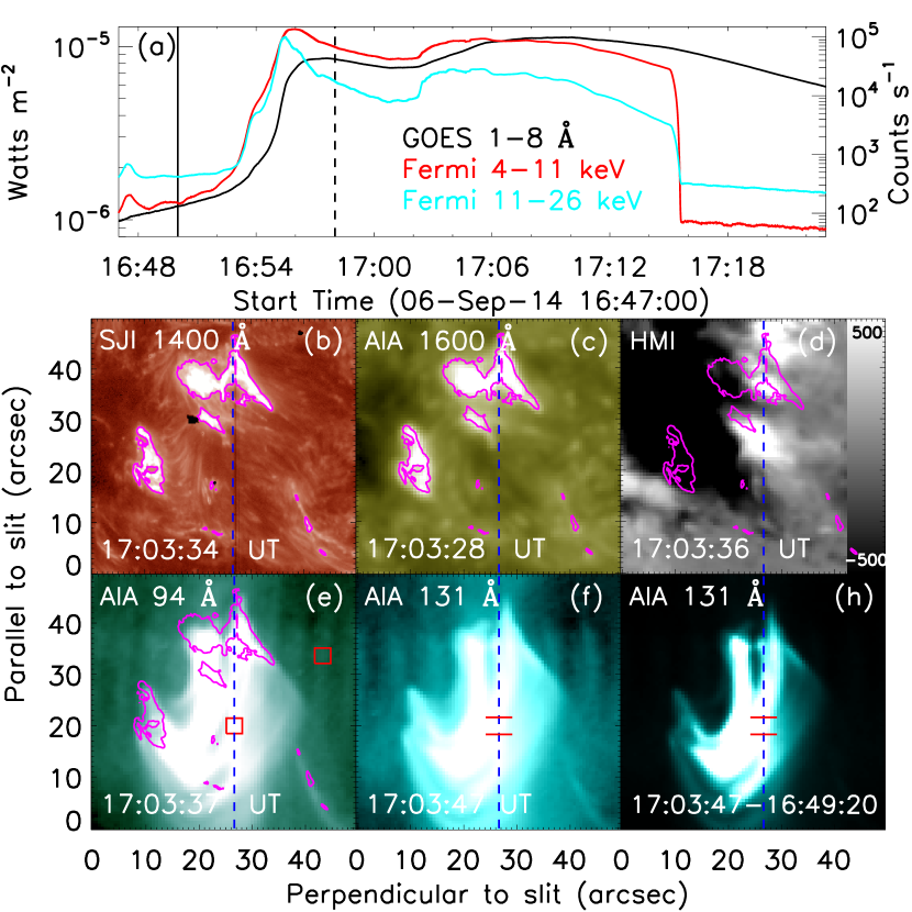
Figure 1: Overview of the solar flare on 2014 September 6. (a) Light curves in GOES 1$-$8 Å (black), Fermi 4$-$11 keV (red) and 11$-$26 keV (turquoise). The vertical line indicates the flare onset time, the dashed line outlines the beginning time of the non-damping oscillations. (b)$-$(f): SJI 1400 Å image, AIA 1600 Å image, HMI LOS magnetogram, AIA 94 Å and 131 Å images. The purple contours are based on the intensity level of SJI 1400 Å image, the HMI image saturates at $\pm$500 G, and the AIA and SJI images are shown in a logarithmic brightness scale. (h): Difference image in AIA 131 Å. The IRIS slit position is marked by blue dashed lines. The red boxes give the regions used in the DEM analysis. Two red bars enclose the flaring loop top used for further analysis. The temporal evolution over $\sim$34 minutes in AIA 94 Å and 131 Å is available as a movie online (movie.mp4), which also contains running difference images in the lower panels.

Figure 1 (b)$-$(f) show the nearly simultaneous snapshots with a same field-of-view (FOV) of about 50$\arcsec$$\times$50$\arcsec$ provided by the IRIS Slit-Jaw Imager (SJI), the HMI line-of-sight (LOS) magnetogram and AIA EUV/UV images. The AIA and HMI images were processed with the solar software (SSW) routines ‘aia_prep.pro’ and ‘hmi_prep.pro’, respectively (Lemen et al., 2012; Schou et al., 2012). The AIA 1600 Å image was used as a reference to co-align with SJI 1400 Å image (Li et al., 2014; Cheng et al., 2015; Li et al., 2016b), because they both contain the main bright features dominant by the continuum emission from the temperature minimum (see the contours). The bottom panels in Figure 1 illustrate that the double flare ribbons rooted at positive and negative polarities (Panel (d)) are connected by a bundle of loop structure (Panel (f)). This agrees well with the standard solar flare model (Carmichael, 1964; Sturrock, 1966; Hirayama, 1974; Kopp & Pneuman, 1976). Figure 1 (h) highlights the loop structure with the difference image taken before and during the flare time in AIA 131 Å band. A bundle of flaring loop structure are visualized, which is very likely to be associated with hot plasma structures at about 11 MK (Lemen et al., 2012). The flaring loop is estimated to have a length of about 48 Mm and a width of about 5.9 Mm; the loop-top reaches a height of about 25$-$35 Mm.

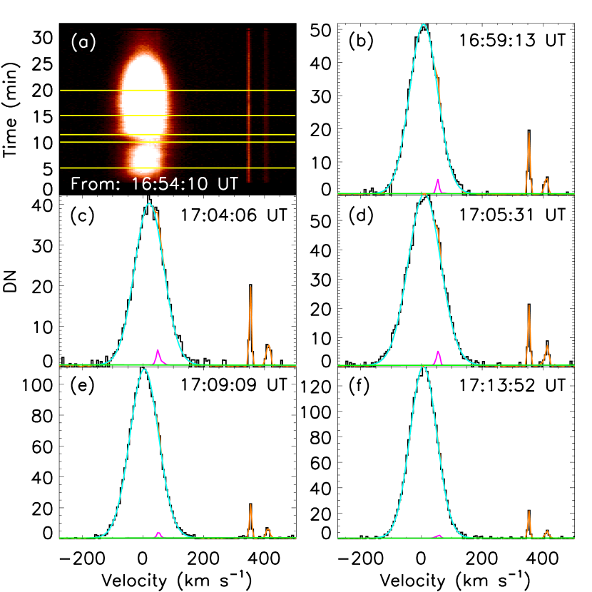
Figure 2: Flaring spectra observed by the IRIS. (a): Time evolution of the line profiles in Fe xxi 1354.08 Å. (b)$-$(f): Spectral line profiles (black) and their double Gaussian fitting results (orange) with a linear background (green) at the time indicated by the yellow lines in panel (a). The turquoise line is Fe xxi 1354.08 Å, and the purple line is C i 1354.29 Å. The zero velocity is set to the rest wavelength of Fe xxi 1354.08 Å.

The IRIS spectra measure the flare in a ‘sit-and-stare’ mode with a roll angle of 45^∘. The spectral scale is $\sim$25.6 mÅ per pixel in the far-ultraviolet (FUV) wavelengths. The IRIS slit crosses the flaring loop and one ribbon (Figure 1). Two red bars enclosed the flaring loop region used to study the quasi-periodic oscillations in this work. IRIS spectrum was pre-processed with the SSW routines of ‘iris_orbitval_corr_l2.pro’ (Tian et al., 2014; Cheng et al., 2015) and ‘iris_prep_despike.pro’ (De Pontieu et al., 2014). To improve the signal-to-noise ratio, we apply a running average over 5 pixels to the IRIS spectra along the slit (Tian et al., 2012, 2016). We also manually perform the absolute wavelength calibration using a relatively strong neutral line, i.e., O i 1355.60 Å (see De Pontieu et al., 2014; Tian et al., 2015; Tian, 2017). IRIS observations show that Fe xxi 1354.08 Å is a hot ($\sim$11 MK) and broad emission line and is always blended with many narrow chromospheric lines at the flaring ribbons (Li et al., 2015b; Tian et al., 2015; Li et al., 2016b; Young et al., 2015; Brosius et al., 2016; Polito et al., 2016). However, the Fe xxi 1354.08 Å line is much stronger than those blended emission lines at the flaring loops (Tian et al., 2016). Figure 2 (a) gives the time evolution of the line profiles of Fe xxi 1354.08 Å, averaged over the slit positions between $\sim$18.3″$-$21.6″. Figure 2 (b)$-$(f) show the spectral line profiles at the time indicated by the yellow lines in panel (a). We can see that only the cool line of C i 1354.29 Å is blended with the hot line of Fe xxi 1354.08 Å, but its contribution is negligible. Therefore, double Gaussian functions superimposed on a linear background are used to fit the IRIS spectra at ‘O i’ window (Tian et al., 2016). Next, we can extract the hot line of Fe xxi 1354.08 Å, as shown by the turquoise profile. The purple profile is the cool line of C i 1354.29 Å. Two orange peaks represent the cool lines of O i 1354.60 Å and C i 1354.84 Å (Tian, 2017), which are far away from the flaring line of Fe xxi 1354.08 Å. Finally, the line properties of Fe xxi 1354.08 Å are extracted from the fitting results, i.e., Doppler velocity, peak intensity and line width (Li et al., 2016b; Tian et al., 2016; Tian & Chen, 2018).

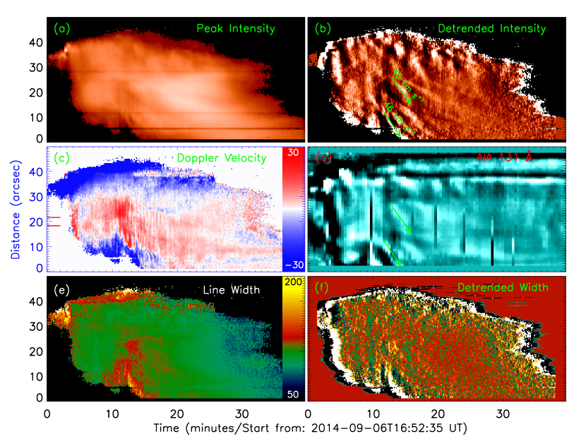
Figure 3: Time-distance plot. Left: The peak intensity image (a) is shown in logarithmic scale, while the unit of color bars in Doppler velocity (c) and line width (e) images is km s^-1. Right: Detrended images in peak intensity (b), AIA 131 Å intensity (d) and line width (f). Two red bars enclose the flaring loop-top region, and the green arrows indicate the propagating directions.

Figure 3 shows the time-distance (TD) images of Fe xxi 1354.08 Å from the IRIS spectral fitting results, including peak intensity (a), Doppler velocity (c), and line width (e). In panel (c), we can clearly see that the Doppler velocities are redshifted in the IRIS slit positions between around 10″$-$30″, and these regions are located at the flaring loops, while the strong blueshifted regions correspond to the flaring ribbons (see Figure 1). The Doppler shift oscillations exhibit two periodic behaviors. One is characterized by a series of vertical slashes with a short period near one minute, another one shows a repeating blobby pattern with a lone period of roughly five minutes. The Doppler shift oscillations with a short period appear at the redshifted wings and tend to drift downward along the IRIS slit, indicating the expansion of flaring loops. The oscillations appear to be largely coherent over a wide range along the slit of IRIS, suggesting the oscillations of a fat flaring loop, or implying that many thin flaring loops oscillate as a whole (Tian et al., 2016). Similar visible oscillations with short period are not detected in the peak intensity and line width. We then plot the detrended images by removing a 3-minute running average (Wang et al., 2009; Tian et al., 2012) of peak intensity (b) and line width (f) in Fe xxi 1354.08 Å, we also give the detrended image in AIA 131 Å (d), which is from the IRIS slit positions. The dark vertical bars at 10, 16, 20, 24, etc. minutes in panel (d) are caused by the long exposure time of AIA. This is because that AIA will change its exposure time when solar flare erupting in EUV bandpasses (Lemen et al., 2012). The detrended images in the peak intensity of Fe xxi and AIA 131 Å show obvious propagating features. The speed is estimated to be about 45 km s^-1, as indicated by the green arrows. This is much smaller than the local sound speed, i.e., about 500 km s^-1 at 11 MK (Nakariakov & Ofman, 2001; Kumar et al., 2013; Li et al., 2017b). It could be associated with intermittently evaporated plasma, see also the movie.mp4, which clearly shows the flaring loops in AIA 94 Å and 131 Å propagating and intermittently passing the slit of IRIS. The detrended image of line width does not show the apparent propagating features.

3 Results

3.1 Time series

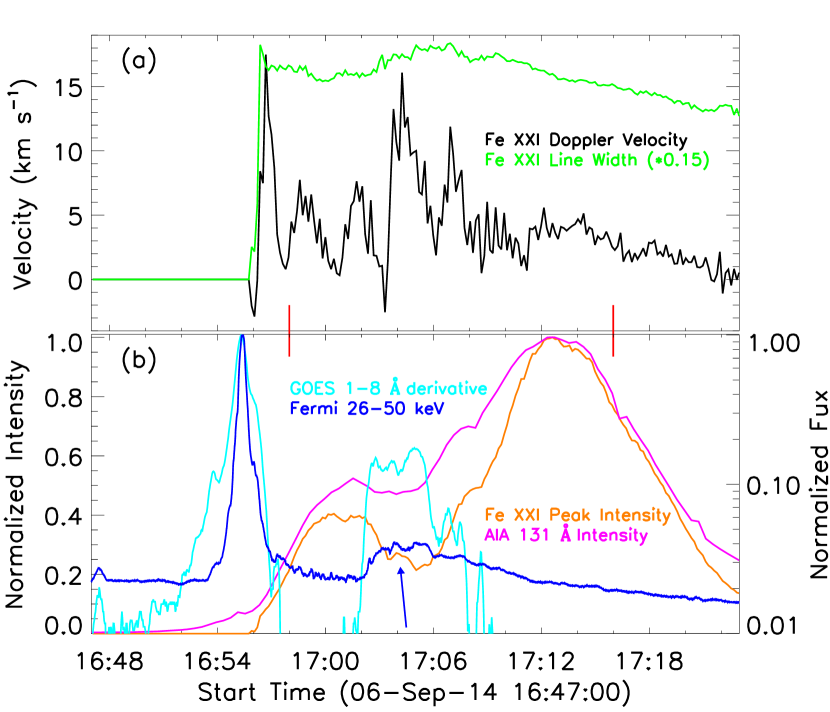
Figure 4: Time-evolution curves. Time series of Doppler velocity (black), line width (green) and peak intensity (orange) in Fe xxi 1354.08 Å, as well as the AIA 131 Å intensity (purple), the light curves in GOES 1$-$8 Å derivative (turquoise) and Fermi 26$-$50 keV (green). The blue arrow indicates a small HXR pulse, and two red vertical ticks outline the detrended time series in Figure 5.

Figure 4 (a) and (b) plot the time series of Doppler velocity (black), line width (green), peak intensity (orange) in Fe xxi 1354.08 Å, as well as the normalized intensity in AIA 131 Å (purple). They are averaged over 20 pixels between 18.3″$-$21.6″ (two red bars in Figures 1 (f, h) and 3 (c)) along the IRIS slit, which cover the pronounced oscillatory behaviors. The primary behavior for the Doppler velocity seems to the oscillations with a period of around 3 minutes, but such oscillations are not visible in the line width, as shown in panel (a). Moreover, the primary oscillations with 3-min period are not pronounced in the Doppler shift image in Figure 3 (c). On the other hand, there are wiggles on both Doppler velocity and line width that are superimposed on their strong backgrounds, respectively. These wiggles might be the small-amplitude oscillations with a period of around one minute, which correspond well with the redshifted vertical slashes in Figure 3 (c). The peak intensity and the AIA 131 Å intensity exhibit two flat peaks, and appear to match well, as shown in panel (b). We also plot the HXR light curves in GOES 1$-$8 Å derivative (turquoise), and Fermi/GBM 26$-$50 keV (blue). Similar to the SXR fluxes in Figure 1 (a), the HXR emissions also exhibit double pulses, but the second pulse is much weaker that the first one, as indicated by the blue arrow. These HXR light curves do not show the pronounced oscillatory behaviors with a periods of about 3 minutes. Similar as that in the Doppler velocity and line width of Fe xxi 1354.08 Å, there are a series of wiggles on these HXR fluxes, which are superimposed on the strong background emissions too.

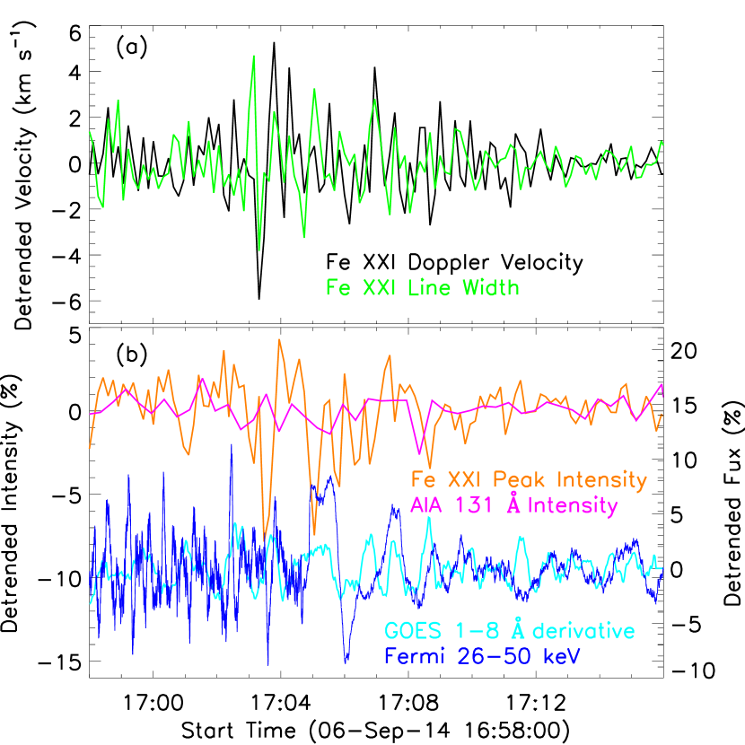
Figure 5: Detrended time-evolution profiles. Detrended time series of the curves in Figure 4 between 16:58 UT$-$17:16 UT.

As described above, the wiggles that might be the small-amplitude oscillations are much weaker than their background emissions, which make them difficult to be identified (Dolla et al., 2012; Li & Zhang, 2017). To make these rapid oscillations more apparent, the detrended Doppler velocity and line width are accomplished by removing the 60 s running average from their time series (Wang et al., 2009; Tian et al., 2012; Li et al., 2017b), since we would enhance the short period oscillation and suppress long period trend (Gruber et al., 2011; Auchère et al., 2016). The 60 s average is selected because that the Doppler shift image in Figure 3 (c) exhibits a series of vertical slashes with a period near one minute. Figure 5 (a) shows that both of the detrended Doppler velocity and line width exhibit the rapid oscillations with small-scale amplitudes. We also give the detrended time series of Fe xxi 1354.08 Å peak intensity (orange) and AIA 131 intensity (purple), as well as the detrended HXR fluxes in GOES 1$-$8 Å (turquoise) derivative and Fermi/GBM 26$-$50 keV (blue), as shown in Figure 5 (b). The detrended HXR fluxes and peak intensity of Fe xxi 1354.08 Å also display the rapid oscillations, their oscillatory amplitudes are small. However, the detrended intensity in AIA 131 Å does not exhibit the similar rapid oscillations, which is caused by the lower time cadence of AIA 131 Å (i.e., 24 s).

3.2 Fourier Spectra and Wavelet Analysis

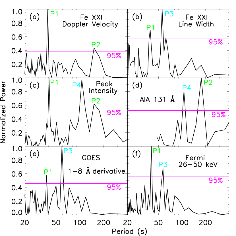
Figure 6: Fourier Spectra. Normalized FFT power spectra of the detrended time series from Doppler velocity (a), line width (b) and peak intensity (c) in Fe xxi 1354.08 Å, AIA EUV (d), GOES derivative (e) and Fermi HXR (f) fluxes. A horizontal purple line in each panel indicates the 95% confidence level.

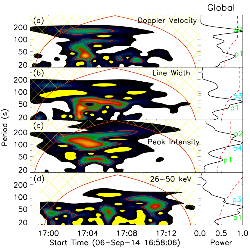
Figure 7: Wavelet analysis results. Wavelet power spectra and global wavelet of the detrended time series from Fe xxi 1354.08 Å Doppler velocity (a), line width (b), and peak intensity (c), as well as Fermi 26$-$50 keV (d). The red lines indicate a significance level of 95%.

To examine the period of flaring loop oscillations, we obtain the Fourier spectra (Figure 6 (a)$-$(f)) with the Lomb-Scargle periodogram (Scargle, 1982; Yuan et al., 2011) for the detrended time series of Doppler velocity, line width, peak intensity in Fe xxi 1354.08 Å, and AIA 131 Å intensity, as well as the detrended HXR fluxes in GOES 1$-$8 Å derivative and Fermi 26$-$50 keV. Then the dominant period is determined from the peak value of the power spectrum, while the error bar is determined as the full-width-at-half-maximum value of the peak power (Yuan et al., 2011; Tian et al., 2016; Li et al., 2017b). Figure 6 (a) shows that there are two distinct peaks above the 95% confidence level (Horne & Baliunas, 1986). Therefore, two prominent periods were obtained in the Doppler velocity of Fe xxi 1354.08 Å, i.e., 40$\pm$3 s (P1), and 155$\pm$15 s (P2). The shorter period (P1) is also detected in the line width and peak intensity of Fe xxi 1354.08 Å, HXR emissions in GOES 1$-$8 Å derivative and Fermi 26$-$50 keV. However, the AIA 131 Å intensity does not exhibit the shorter period (P1), because of its lower cadence (24 s). On the other hand, the longer period (P2) is observed in the Doppler velocity, peak intensity of Fe xxi 1354.08 Å, and AIA 131 Å intensity. Besides the two dominant periods, we also detect another two periods from the power spectrum. For example, a period (P3 = 55$\pm$5 s) is identified in the line width of Fe xxi 1354.08 Å, as well as in the HXR emissions in GOES 1$-$8 Å derivative and Fermi 26$-$50 keV. Another period (P4=110$\pm$10 s) is found in the peak intensity of Fe xxi 1354.08 Å, and AIA 131 Å intensity.

We also perform wavelet analysis (Torrence & Compo, 1998; Yuan et al., 2011; Deng et al., 2012; Tian et al., 2016) on the detrended time series of Doppler velocity, line width, peak intensity in Fe xxi 1354.08 Å and the detrended HXR fluxes in Fermi 26$-$50 keV. Figure 7 gives their wavelet power spectra (left) and global wavelet (right), respectively. They show the similar periods as the Fourier analysis results, and the major oscillations occurs from 17:00 UT to 17:12 UT; this is the time after the first SXR peak or HXR pulse. However, the dominant periods in the wavelet power spectra and global wavelet spectra are always with a broad band, which make some close periods mixing together, such as P1 and P3 in panels (b) and (d), P2 and P4 in panel (c). The oscillatory amplitudes, determined with the square root of the peak global wavelet power, are 2.2 km s^-1 for the Doppler velocity, 1.9 km s^-1 for the line width, and 3.6% for the peak intensity.

3.3 Cross-correlation and DEM Analysis

The cross-correlation analysis (Deng et al., 2013; Tian et al., 2016) is applied to investigate the time lag between Doppler velocity and peak intensity in Fe xxi 1354.08 Å, as shown by the red line in Figure 8 (a). A maximum correlation coefficient is found at the time lag of about 10 s. The maximum correlation is associated with the 40 s oscillatory signal, so the time lag corresponds to a phase shift of about $\pi$/2. Our finding in a hot flaring line is similar to those in the warm coronal emission lines (Tian et al., 2012). Moreover, the same phase shift ($\pi$/2) can also be found between the Doppler velocity signal in the Fe xxi 1354.08 Å line and the detrended HXR fluxes in Fermi 26$-$50 keV (turquoise line). On the other hand, the maximum correlation coefficient is found at the time lag of around 0 s between the detrended time series of Doppler velocity and line width in Fe xxi 1354.08 Å (black line), indicating that the line width oscillates in phase with the Doppler velocity. The same phase oscillations can also be detected between the peak intensity in Fe xxi 1354.08 Å and HXR fluxes in 26$-$50 keV, as seen in the green line.

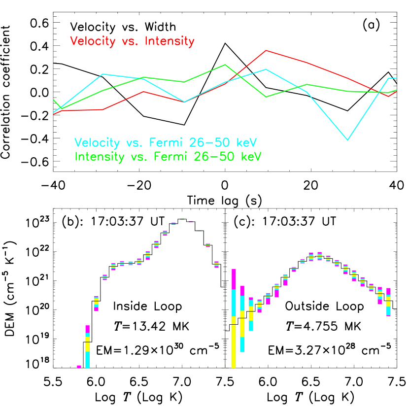
Figure 8: Cross-correlation and DEM analysis results. (a): Correlation coefficient (cc.) between two parameters as a function of time lag. (b) and (c): DEM profiles in the flaring loop (b) and background corona (c) marked by the red boxes in Figure 1. The black profile is the best-fitted DEM curve from AIA observations. The rectangles with different colors on the DEM plot encompass 95% (purple), 80% (turquoise), and 50% (yellow) of the Monte Carlo solutions, respectively. The mean temperature, EM and observed time are labeled in each panel.

Using AIA intensity images in six EUV bandpasses, a differential emission measure (DEM) analysis (Cheng et al., 2012; Shen et al., 2015) is performed for the solar flare at 17:03:37 UT, when the oscillations are pronounced. Figure 8 (b) and (c) plot the DEM profiles in the flaring loop and the background corona, respectively. They contain the same region with an FOV of 3″$\times$3″, as enclosed by the red boxes in Figure 1 (e). The black profile in each panel is the best-fit DEM solution to the observed fluxes. The colored rectangles represent the errors of the DEM curve, which are calculated from 100 Monte Carlo (MC) realizations of the observational data (Cheng et al., 2012; Tian et al., 2016; Li et al., 2017b). The average temperature ($T$) and EM inside and outside (background corona) of the flaring loop are also estimated according to their errors, respectively. For example, the confident temperature (log $T$) range inside the flaring loop is 6.0$-$7.5, while that outside of the flaring loop is 5.8$-$7.1, since the temperature in solar flare are much higher than that in the background corona. Therefore, the number density inside the flaring loop can be estimated with $n_{e}=\sqrt{EM/w}$ by assuming a filling factor of 1.0 (Tian et al., 2016; Li et al., 2017b). And we can obtain a lower limited density inside the flaring loop of $\sim$4.7$\times$10¹⁰ cm^-3. On the other hand, the effective LOS depth ($l\approx\sqrt{H\pi r}\sim 4\times 10^{10}$ cm), instead of the loop width, is applied to calculate the number density outside of the flaring loop (Zhang & Ji, 2014; Zucca et al., 2014; Su et al., 2016; Li et al., 2017b), and we get 9.1$\times$10⁸ cm^-3. Finally, a number density ratio ($r_{d}=n_{0}/n_{e}$) of $\sim$ 0.02 between outside and inside of the flaring loop is determined, this is very close to the density contrast from recent observations (Tian et al., 2016; Li et al., 2017b).

3.4 Magnetic field modeling

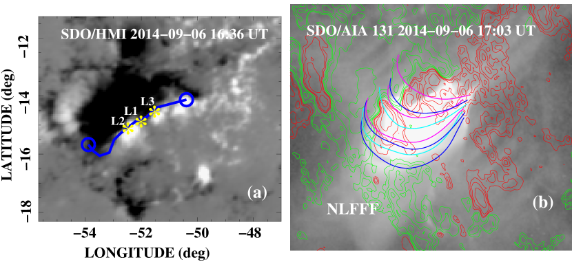
Figure 9: Magnetic field strength estimated from the NLFFF model. (a): Zoomed view of the longitude–latitude map of the radial component of the photospheric magnetic field by SDO/HMI in the HIRES region at 16:36 UT on 2014 September 6. The blue curve with circles at the two ends refers to the path along which we insert the flux rope. (b): Selected field lines from the NLFFF model overlaid on a flare image by AIA, and the red (green) contours refer to the positive (negative) photospheric magnetic fields by HMI. (c): The distributions of the magnetic field strength from this model with height at three locations, i.e., L1, L2 and L3 (marked with yellow stars on panel (a)).

To determine the magnetic field strength of the flaring loops, we construct magnetic field models using the flux rope insertion method developed by van Ballegooijen (2004). We briefly introduce the method below, for detailed descriptions please refer to Bobra et al. (2008); Su et al. (2009, 2011). At first, a potential field model is computed from the high-resolution (HIRES) and global magnetic maps observed by SDO/HMI. The lower boundary condition for the HIRES region is derived from the photospheric line-of-sight magnetograms obtained at 16:36 UT on 2014 September 6. The longitude-latitude map of the radial component of the magnetic field in the HIRES region is presented in Figure  9 (a). The HIRES computational domain extends about 29^∘ in longitude, 28^∘ in latitude, and up to 1.7R_⊙ from the Sun center. The models use variable grid spacing to achieve high spatial resolution in the lower corona (i.e., 0.001R_☉) while covering a large coronal volume in and around the target region. Next we modify the potential field to create cavities in the region above the selected path marked with a blue curve, then insert one thin flux bundle (representing the axial flux $\Phi_{\rm axi}$ of the flux rope) into the cavities. Circular loops are added around the flux bundle to represent the poloidal flux $F_{\rm pol}$ of the flux rope. The resulted magnetic fields are not in force-free equilibrium. We then use the magneto-frictional relaxation to drive the field towards a force-free state (van Ballegooijen et al., 2000; Yang et al., 1986).

We construct a series of magnetic field models by varying the axial and poloidal fluxes of the inserted flux ropes. One of the best-fit non-linear force-free field (NLFFF) models is presented in Figure  9 (b). The inserted flux bundle has the poloidal flux of 0 Mx cm^-1, and the axial flux is 4$\times 10^{20}$ Mx. We can see that selected model field lines match the observed post flaring loops well. The distributions of the magnetic field strength from this model with height at three locations, i.e., L1, L2 and L3 are presented in Figure  9 (c). We can see that the difference of the magnetic strength at these three locations is decreasing with height. They all reach more than 100 G at a height of $\sim$35 Mm above the photosphere. Similar results are also obtained from the potential field model.

4 Discussions

Four distinct periods are identified from the FFT power spectra, as shown in Figure 6. The short periods (P1 and P3) can be detected simultaneously by the IRIS (a, b, c), GOES (e) and Fermi/GBM (f), which could exclude the instrument affects. Moreover, they can be clearly seen as a series of vertical slashes near one minute in the redshifted wing of Doppler velocity image (Figure 3 c). On the other hand, such small-scale oscillations have been reported using the Hinode/EIS or IRIS observations (see., Kitagawa et al., 2010; Tian et al., 2012, 2016), which indicated that we could detect the small-amplitude oscillations, especially in the Doppler velocity images. The longer periods (P2 and P4) can also be observed simultaneously by IRIS and SDO/AIA. They are the primary behaviors for the time series of Doppler velocity (black line) in Figure 4 (a), which seem to oscillations with a period of about 2-3 minutes. Therefore, these periods obtained by the FFT method are reliable.

Usually, quasi-periodic oscillations observed in the impulsive phase of a solar flare are thought to be modulated by the injection of nonthermal electrons accelerated by the quasi-periodic magnetic reconnection (e.g., Dolla et al., 2012; Li et al., 2015a). However, the quasi-periodic oscillations in this study are more likely to be associated with MHD waves, as they are detected after the first HXR pulse, which endures the passage from impulsive to decay phases of a solar flare. The phase speed of the non-damping oscillations ($c_{p}=2L/P$) could be estimated to be $\sim$1200 km s^-1, which is larger than the local sound speed ($\sim$500 km s^-1) at 11 MK. Therefore, they are not the standing slow waves. The sausage waves can be excluded. Because they are often thought to have no Doppler shift oscillations (Kitagawa et al., 2010), or that the line width oscillation period is half of the intensity/velocity oscillation period (Jess et al., 2008). On the other hand, the kink waves can be detected in the intensity disturbances when the LOS is not perpendicular with loop displacement (Tian et al., 2012; Wang et al., 2012; Zimovets & Nakariakov, 2015; Yuan & Van Doorsselaere, 2016b). Figure 1 shows that the slit of IRIS is not exactly perpendicular with the flaring loop, thus we can observe the quasi-periodic oscillations (P1) from the Doppler velocity, the line width, and the peak intensity in Fe xxi 1354.08 Å. The quasi-periodic oscillations in the line width of Fe xxi 1354.08 Å indicate the temporal variations in temperature broadening of the iron line. The analysis from cross-correlation reveals a $\pi$/2 phase shift between Doppler velocity and peak intensity signals, which may be caused by the periodic crossing of the flaring loops over the IRIS slit (Tian et al., 2012, 2016). The quasi-periodic oscillations can also be clearly seen from the HXR emissions in GOES 1$-$8 Å derivative and Fermi 26$-$50 keV. These HXR fluxes integrated over the entire Sun are also found to be in-phase oscillations with the spatially resolved peak intensity in Fe xxi 1354.08 Å (Figure 8 (a)). The kink wave on a coronal loop observed in the HXR emission was often observed as the back and forth movement of a x-ray source. However, it can be connected with the electron acceleration which modulated by kink oscillations of a flaring loop, or with interaction of a flaring loop with another loop which performs kink oscillations. Thus, the reconnection field is periodically fed to the reconnection site by the kink oscillations (Nakariakov & Verwichte, 2005). All these clues suggest that the quasi-periodic oscillations with a short period (P1) at flaring loops are most likely to be the global kink mode (Uchida, 1970; Asai et al., 2001; Tian et al., 2016).

The global kink oscillations with a period of $\sim$40 s are observed simultaneously from the line properties of a flaring line in Fe xxi 1354.08 Å. And their amplitudes are not damped significantly. This is similar as the kink oscillations detected in Doppler velocity at redshifted wings in the warm coronal lines (Tian et al., 2012). Both observations find that the kink oscillations in the peak intensity and line width exhibit a very small oscillatory amplitude. This also explains that the time-distance images of peak intensity and line width do not display the obvious oscillations as that of Doppler velocity, because those oscillations overlap on the strong background (see also., Dolla et al., 2012; Li et al., 2017b). Our new observational result is that the kink oscillations within non-damping amplitudes are identified at hot flaring loops, i.e., 11 MK. To our knowledge, the non-damping kink oscillations in a hot flaring line (e.g., Fe xxi 1354.08 Å) have never been reported. Previous reports of kink oscillations were mainly observed in the warm ($<$10 MK) coronal lines (Tian et al., 2012; Wang et al., 2012) or EUV images (Su et al., 2012; Goddard & Nakariakov, 2016; Yuan & Van Doorsselaere, 2016a). Thanks to the high-resolution observations from the IRIS, we can investigate the non-damping kink oscillations in a hot line of Fe xxi 1354.08 Å at flaring loops.

Previous observations showed that the period of kink oscillations were usually larger than 60 s, and even tens of minuets. However, these longer periods of kink oscillations were observed from the imaging observations in EUV/SXR passbands (Nakariakov et al., 1999; Aschwanden et al., 2002; Yuan & Van Doorsselaere, 2016a) or the spectroscopic observations in the warm coronal lines (Tian et al., 2012). Actually, the kink oscillations with a short period of 6.6 s have been reported by Asai et al. (2001) using the Nobeyama Radioheliograph. And a 43 s periodicity is found by Koutchmy et al. (1983) in the Doppler velocity of the Fe xiv 5303 Å line, which is interpreted as a standing kink wave (Roberts et al., 1984). All those periods of kink oscillations are less than 60 s, which are similar as our results. On the other hand, the oscillatory amplitude of peak intensity in Fe xxi 1354.08 Å is smaller than 3.6%, and they are not damped. This is consistent with the non-damping kink oscillations of coronal loops observed in AIA/EUV images, which also have smaller amplitudes but can last for tens of cycles (e.g., Anfinogentov et al., 2013; Nisticò et al., 2013; Anfinogentov et al., 2015). Therefore, the short period of kink oscillations at hot flaring loops is reasonable, because the hot flaring loops are much shorter that the warm coronal loops (Aschwanden et al., 2002; Anfinogentov et al., 2015).

Another short period (P3) of $\sim$55 s could also be the kink oscillations, and it is very close to the period of P1. In the wavelet power spectra, they are even mixing together and difficult to distinguish. The small difference between these two periods might be caused by the expansion of the flaring loops with time (Verth & Erdélyi, 2008; Tian et al., 2016). Based on the model of kink oscillations, we can estimate the magnetic fields at flaring loops from Equation 1 (Roberts et al., 1984; Nakariakov & Ofman, 2001; Nakariakov & Verwichte, 2005; Nakariakov & Melnikov, 2009; Tian et al., 2012; Yuan & Van Doorsselaere, 2016a).

$$B\approx 4.6\times 10^{-12}\frac{L}{P_{k}}\sqrt{2n_{e}(1+r_{d})}$$ (1)

As mentioned above, the length of flaring loop (L), the number density in flaring loops, and the density ratio ($r_{d}$) between outside and inside flaring loops have been obtained, which are $\sim$48 Mm, $\sim$4.7$\times$10¹⁰ cm^-3, and $\sim$0.02, respectively. Therefore, the magnetic fields at flaring loops can be estimated from the periods ($P_{k}\sim 40-55\leavevmode\nobreak\ s$) of kink oscillations, which are about 120$-$170 G. This is consistent with the magnetic field modeling results, i.e., 110$-$180 G at a height of $\sim$25$-$35 Mm above the photosphere (see., Figure 9c). Our results are also similar as previous findings obtained by Qiu et al. (2009).

The longer periods of about 155 s and 110 s are clearly seen in the peak intensity of Fe xxi 1354.08 Å and AIA 131 Å intensity. They are propagating with a speed of $\sim$45 km s^-1 (Figure 3). The period of around 155 s can also be observed in the Doppler velocity of Fe xxi 1354.08 Å, and they are always oscillating in the redshifted wings, which might be related to the enhancement of downflows in flaring loops after ‘chromospheric evaporation’ (Tian et al., 2015; Li et al., 2017c). However, these longer periods are missed by the HXR fluxes in GOES 1$-$8 Å derivative and Fermi 26$-$50 keV. Therefore, these longer periods are impossibly considered to be the MHD waves. They are most likely the recurring downflows in flaring loops, which are caused by the flaring loops periodically crossing the slit of IRIS (Tian et al., 2012, 2016). The two domain periods in the intensity of Fe xxi 1354.08 Å and AIA 131 Å are probably due to the flaring loop expansions.

5 Summary

Using the observational data from IRIS, SDO, GOES and Fermi, we explore the non-damping oscillations with a short period of $\sim$40 s in a hot flaring line of Fe xxi 1354.08 Å, which can be detected in the Doppler velocity, the line width, the peak intensity of Fe xxi 1354.08 Å and also the HXR fluxes in GOES 1$-$8 Å derivative and Fermi 26$-$50 keV. A $\pi$/2 phase shift between the detrended time series of the Doppler velocity and peak intensity (and HXR fluxes) is found, while the Doppler velocity and line width are found to be oscillating in phase. The oscillatory amplitudes of the Doppler velocity and the line width are identified to be 2.2 km s^-1, and 1.9 km s^-1, respectively. While that of the peak intensity is less than 3.6% related to their background trend. A longer period of $\sim$155 s is observed in the Doppler velocity, the peak intensity of Fe xxi 1354.08 Å, and also the AIA 131 Å intensity, which is mostly likely the recurring downflows at hot flaring loops rather than the MHD waves.