Real-Time Equality-Constrained Hybrid State Estimation in Complex Variables

Abstract

The hybrid power system state estimation problem requires computing the state of the power network using data from both legacy and phasor measurements. Recent research has shown that the normal equations approach in complex variables is computationally advantageous, particularly in the presence of phasor measurement values, and that its software implementation is best suited to modern processors that employ single instruction multiple data (SIMD) processor extensions. The complex normal equations approach is however not ideal for handling zero injection measurements, as it requires their modeling as pseudo-measurements with high weights. This paper employs Wirtinger calculus for extending the complex normal equations approach to include equality constraints, and contrasts it with two previously published implementations: the normal equations approach in complex variables and the hybrid equality constrained state estimator in real variables. Numerical results are reported on transmission networks having up to 9241 nodes; they show that the complex variable equality constrained hybrid state estimator exhibits superior performance as compared to the above two techniques in terms of both computational time and accuracy. Moreover, the execution time on the largest network is less than 300 ms, which makes the proposed implementation commensurate with the requirements of real-time applications.

I Introduction

The power system state estimation problem is most commonly formulated as a weighted least squares problem and solved via the normal equations (NE) approach; the main advantage of the NE approach is that it gives rise to a gain matrix that can be rapidly factorized using sparsity techniques. Nodes that have neither generation nor load are modeled as virtual zero complex power injection measurements, which are very useful to enhance the estimation accuracy. Zero injection measurements can be accounted for in the NE approach by assigning relatively much larger weights to them, but this can potentially cause ill-conditioning. It is now accepted that zero injections are best handled through formulating the estimation problem as an equality constrained optimization program, leading to methods such as the normal equations with equality constraints, Hatchel’s augmented matrix method, and other hybrid forms and extensions [1, 2, 3].

In the current operational practice, state estimators are expected to employ measurements from both the supervisory control and data acquisition (SCADA) and the phasor measurement unit (PMU) systems. PMU measurements are increasingly being employed in power systems, with benefits in risk mitigation against cyber attacks [4], in Volt-VAr control [5], and in transmission network state estimation [6]. Handling phasor current measurements in power grid state estimation can be accomplished using either noninvasive or direct techniques. The noninvasive methods have the distinct advantage of not requiring any update to the classical state estimator implementations that are based on SCADA measurements; they rather employ post processing techniques that improve the estimation outcome by fusing the SCADA measurement-based state vector with the PMU measurements [7, 8, 9, 10, 11, 12]. Noninvasive methods however require complete observability by the SCADA telemetering system. On the other hand, the direct techniques do not necessitate SCADA system observability, but rather treat both SCADA and PMU measurements in a unified optimization framework [13, 14, 15]. The large disparity in data refresh rates amongst PMU and SCADA measurements is an issue common to all hybrid state estimators; the proposed solutions include buffering PMU measurements [16] and SCADA state reconstruction techniques [17, 18].

Recent research has shown that hybrid state estimation can be carried out using the NE approach in complex variables [19], and that the complex variable approach has advantages (i) in handling complex-valued measurements and (ii) in implementation on modern processors that support single instruction multiple data (SIMD) operations [20]. SIMD instructions allow processing multiple pieces of data using a single instruction, thus speeding up the throughput of implementations for video encoding/decoding, image processing, and data analysis [21]; SIMD instruction sets also allow fused multiply-accumulate operations, which could naturally be leveraged in complex variable computing applications. The complex NE (CNE) approach in [19] is a generalization of the real variable implementation, derived via Wirtinger calculus [22, 23]. This paper extends the CNE approach to include equality constraints, and thus effectively handle zero injection measurements for further improving the estimation accuracy; the complex equality constrained (CEC) estimator is implemented using advanced vector extensions (AVX-2) [21] and contrasted with both the CNE approach [19] and the real equality constrained (REC) hybrid state estimator [15].

The rest of this paper is organized as follows. Section II reviews the normal equations approach in complex variables, and Section III presents the extension to the complex variable normal equations with equality constraints. An introduction to the program implementation via AVX-2 is given in Section IV. Section V presents numerical results and comparisons with the CNE [19] and REC [15] estimators on networks with up to 9241 nodes. The paper is concluded in Section VI.

II Complex Normal Equations (CNE)

Consider the power system state estimation problem in complex variables (1), where $h(x,\overline{x})$ is the vector of measurement functions, $z$ is the vector of measured values, $x$ is the vector of complex state variables (phasor voltages), and $\overline{x}$ denotes the conjugate of $x$ [19]:

$$h(x,\overline{x})\thickapprox z$$ (1)

$$h(x,\overline{x})=\left[\begin{array}[]{c}h_{1}(x,\overline{x})\\ \vdots\\ h_{m}(x,\overline{x})\end{array}\right],\quad z=\left[\begin{array}[]{c}z_{1}\\ \vdots\\ z_{m}\end{array}\right]$$ (2)

Using Wirtinger calculus, (1) can be linearized via the complex Taylor series expansion around the current estimate of the state vector $\left[x^{*};\overline{x}^{*}\right]$; $H$ is formed by the Jacobian $H_{x}$ and the conjugate Jacobian $H_{\overline{x}}$ matrices evaluated at $\left[x^{*};\overline{x}^{*}\right]$:

$$h(x^{\star},\overline{x}^{\star})+H\left[\begin{array}[]{c}\Delta x\\ \Delta\overline{x}\end{array}\right]\approx z$$ (3)

$$H=\left[H_{x},H_{\overline{x}}\right]=\left[\begin{array}[]{cccccc}\frac{\partial h_{1}}{\partial x_{1}}&\cdots&\frac{\partial h_{1}}{\partial x_{n}}&\frac{\partial h_{1}}{\partial\overline{x}_{1}}&\cdots&\frac{\partial h_{1}}{\partial\overline{x}_{n}}\\ \vdots&\ddots&\vdots&\vdots&\ddots&\vdots\\ \frac{\partial h_{m}}{\partial x_{1}}&\cdots&\frac{\partial h_{m}}{\partial x_{n}}&\frac{\partial h_{m}}{\partial\overline{x}_{1}}&\cdots&\frac{\partial h_{m}}{\partial\overline{x}_{n}}\end{array}\right]$$ (4)

The correction to the state vector $\left[\Delta x^{*};\Delta\overline{x}^{*}\right]$ is obtained by minimizing the weighted least squares (WLS) objective value:

$$\ell(\Delta x,\Delta\overline{x})=\frac{1}{2}\left(\overline{r}-\overline{H}\left[\begin{array}[]{c}\Delta\overline{x}\\ \Delta x\end{array}\right]\right)^{T}W\left(r-H\left[\begin{array}[]{c}\Delta x\\ \Delta\overline{x}\end{array}\right]\right)$$ (5)

where $W$ is a diagonal matrix of measurement weights and $r=z-h(x^{\star},\overline{x}^{\star})$. Eq. (5) can be expanded into (6), with the vector $\beta$ and matrix $G$ given by (7) and (8), respectively:

$$\ell =\frac{1}{2}\left(\overline{r}^{T}Wr-\overline{\beta}^{T}\left[\begin{array}[]{c}\Delta x\\ \Delta\overline{x}\end{array}\right]-\left[\begin{array}[]{cc}\Delta\overline{x}^{T}&\Delta x^{T}\end{array}\right]\beta\right)$$ (6)

$$+\frac{1}{2}\left(\left[\begin{array}[]{cc}\Delta\overline{x}^{T}&\Delta x^{T}\end{array}\right]G\left[\begin{array}[]{c}\Delta x\\ \Delta\overline{x}\end{array}\right]\right)$$

$$\beta=\overline{H}^{T}Wr=\left[\begin{array}[]{c}\beta_{\overline{x}}\\ \beta_{x}\end{array}\right]$$ (7)

$$G=\overline{H}^{T}WH=\left[\begin{array}[]{cc}G_{\overline{x}x}&G_{\overline{xx}}\\ G_{xx}&G_{x\overline{x}}\end{array}\right]$$ (8)

Ref. [19] shows that for hybrid power system state estimation, the elements of $G$ and $\beta$ satisfy the following properties: $\beta_{x}=\overline{\beta}_{\overline{x}}$, $G_{x\overline{x}}=\overline{G}_{\overline{x}x}=G_{\overline{x}x}^{T}$, and $G_{xx}=G_{xx}^{T}=\overline{G}_{\overline{xx}}=\overline{G}_{\overline{xx}}^{T}$. Then the minimizer of (6) is given by the solution of the normal equations:

$$G\left[\begin{array}[]{c}\Delta x\\ \Delta\overline{x}\end{array}\right]=\beta$$ (9)

III Complex Equality Constrained (CEC) Normal Equations

The zero injection measurements give rise to a large disparity of weights in the normal equations approach, and may lead to severe ill-conditioning [1]. This problem can be alleviated by a constrained WLS method, which treats zero injection measurements as equality constraints. The zero injection at node $i$ is modeled by the complex power injection ($s_{i}(x,\overline{x})=0$) and its conjugate ($\overline{s}_{i}(x,\overline{x})=0$), leading to the following relationship between their Wirtinger derivatives [23]:

$$\frac{\partial\overline{s}_{i}}{\partial x_{j}}=\overline{\left(\frac{\partial s_{i}}{\partial\overline{x}_{j}}\right)},\quad\frac{\partial\overline{s}_{i}}{\partial\overline{x}_{j}}=\overline{\left(\frac{\partial s_{i}}{\partial x_{j}}\right)}$$ (10)

Therefore, the constrained linear WLS problem can be written as:

$$\min\ell(\Delta x,\Delta\overline{x})$$ (11)

subject to:

$$J\left[\begin{array}[]{c}\Delta x\\ \Delta\overline{x}\end{array}\right]=\left[\begin{array}[]{cc}J_{x}&J_{\overline{x}}\\ \overline{J}_{\overline{x}}&\overline{J}_{x}\end{array}\right]\left[\begin{array}[]{c}\Delta x\\ \Delta\overline{x}\end{array}\right]=\left[\begin{array}[]{c}-s\\ -\overline{s}\end{array}\right]$$ (12)

where the elements in the complex vectors $s$ and $\overline{s}$ contain the equations for the zero complex power injections and their conjugates, except for the last element in each vector that sets the slack angle condition; the corresponding equations are given in the Appendix. The classical theory of Lagrange multipliers for solving constrained minimization problems stipulates that the objective function and constraints are real-valued functions of real unknown variables; however by applying Wirtinger calculus, [23] shows that a stationary point of the Lagrangian function (13) is a solution to (11)-(12), where $\Re$ denotes the real part of a complex quantity:

$$\mathcal{L=}\ell(x,\overline{x})+\Re\left\{\left[\overline{\lambda}^{T},\lambda^{T}\right]\left(\left[\begin{array}[]{cc}J_{x}&J_{\overline{x}}\\ \overline{J}_{\overline{x}}&\overline{J}_{x}\end{array}\right]\left[\begin{array}[]{c}\Delta x\\ \Delta\overline{x}\end{array}\right]+\left[\begin{array}[]{c}s\\ \overline{s}\end{array}\right]\right)\right\}$$ (13)

Theorem 1.

The solution to the complex constrained linear WLS problem (11)-(12) that arises in hybrid power system state estimation is given by the normal equations with equality constraints:

$$\left[\begin{array}[]{cccc}G_{\overline{x}x}&G_{\overline{xx}}&\overline{J}_{x}^{T}&J_{\overline{x}}^{T}\\ \overline{G}_{\overline{xx}}&\overline{G}_{\overline{x}x}&\overline{J}_{\overline{x}}^{T}&J_{x}^{T}\\ J_{x}&J_{\overline{x}}&0&0\\ \overline{J}_{\overline{x}}&\overline{J}_{x}&0&0\end{array}\right]\left[\begin{array}[]{c}\Delta x\\ \Delta\overline{x}\\ \lambda\\ \overline{\lambda}\end{array}\right]=\left[\begin{array}[]{c}\beta_{\overline{x}}\\ \overline{\beta}_{\overline{x}}\\ -s\\ -\overline{s}\end{array}\right]$$ (14)

Proof:

Eq. (22) shows that the function in parenthesis in (13) is real:

$$\left[\overline{\lambda}^{T},\lambda^{T}\right]\left(\left[\begin{array}[]{cc}J_{x}&J_{\overline{x}}\\ \overline{J}_{\overline{x}}&\overline{J}_{x}\end{array}\right]\left[\begin{array}[]{c}\Delta x\\ \Delta\overline{x}\end{array}\right]+\left[\begin{array}[]{c}s\\ \overline{s}\end{array}\right]\right) =$$ (21)

$$\underset{2\Re\left\{\overline{\lambda}^{T}J_{x}\Delta x\right\}}{\underbrace{\overline{\lambda}^{T}J_{x}\Delta x+\lambda^{T}\overline{J}_{x}\Delta\overline{x}}}+\underset{2\Re\left\{\overline{\lambda}^{T}J_{\overline{x}}\Delta\overline{x}\right\}}{\underbrace{\overline{\lambda}^{T}J_{\overline{x}}\Delta\overline{x}+\lambda^{T}\overline{J}_{\overline{x}}\Delta x}}+\underset{2\Re\left\{\overline{\lambda}^{T}s\right\}}{\underbrace{\overline{\lambda}^{T}s+\lambda^{T}\overline{s}}}$$ (22)

Using (22), the Lagrangian function (13) reduces to:

$$\mathcal{L=}\ell(x,\overline{x})+\left[\overline{\lambda}^{T},\lambda^{T}\right]\left(\left[\begin{array}[]{cc}J_{x}&J_{\overline{x}}\\ \overline{J}_{\overline{x}}&\overline{J}_{x}\end{array}\right]\left[\begin{array}[]{c}\Delta x\\ \Delta\overline{x}\end{array}\right]+\left[\begin{array}[]{c}s\\ \overline{s}\end{array}\right]\right)$$ (23)

Therefore:

$$\nabla_{\Delta\overline{x}}\mathcal{L} =\nabla_{\Delta\overline{x}}\ell+\left[\overline{\lambda}^{T}J_{\overline{x}}+\lambda^{T}\overline{J}_{x}\right]^{T}$$

$$=-\beta_{\overline{x}}+G_{\overline{x}x}\Delta x+G_{\overline{xx}}\Delta\overline{x}+\overline{J}_{x}^{T}\lambda+J_{\overline{x}}^{T}\overline{\lambda}$$ (24)

$$\nabla_{\Delta x}\mathcal{L} =\nabla_{\Delta x}\ell+\left[\overline{\lambda}^{T}J_{x}+\lambda^{T}\overline{J}_{\overline{x}}\right]^{T}$$

$$=-\overline{\beta}_{\overline{x}}+\overline{G}_{\overline{xx}}\Delta x+\overline{G}_{\overline{x}x}\Delta\overline{x}+\overline{J}_{\overline{x}}^{T}\lambda+J_{x}^{T}\overline{\lambda}$$ (25)

Equating (24) and (25) to zero, together with the feasibility constraints (12), results in a set of equations that is necessary and sufficient to compute a stationary point of $\mathcal{L}$ (a minimizer of (11)-(12) due to the convexity of the problem); these conditions are given in (14). It stays to demonstrate that the solution to (14) gives two pairs of complex conjugate vectors, $\left[\Delta x;\Delta\overline{x}\right]$ and $\left[\lambda;\overline{\lambda}\right]$. To show this, write (14) as:

$$\left[\begin{array}[]{cccc}G_{\overline{x}x}&G_{\overline{xx}}&\overline{J}_{x}^{T}&J_{\overline{x}}^{T}\\ \overline{G}_{\overline{xx}}&\overline{G}_{\overline{x}x}&\overline{J}_{\overline{x}}^{T}&J_{x}^{T}\\ J_{x}&J_{\overline{x}}&0&0\\ \overline{J}_{\overline{x}}&\overline{J}_{x}&0&0\end{array}\right]\left[\begin{array}[]{c}\Delta x\\ \Delta y\\ \lambda\\ \mu\end{array}\right]=\left[\begin{array}[]{c}\beta_{\overline{x}}\\ \overline{\beta}_{\overline{x}}\\ -s\\ -\overline{s}\end{array}\right]$$ (26)

Taking the complex conjugate of (26) gives:

$$\left[\begin{array}[]{cccc}\overline{G}_{\overline{x}x}&\overline{G}_{\overline{xx}}&J_{x}^{T}&\overline{J}_{\overline{x}}^{T}\\ G_{\overline{xx}}&G_{\overline{x}x}&J_{\overline{x}}^{T}&\overline{J}_{x}^{T}\\ \overline{J}_{x}&\overline{J}_{\overline{x}}&0&0\\ J_{\overline{x}}&J_{x}&0&0\end{array}\right]\left[\begin{array}[]{c}\Delta\overline{x}\\ \Delta\overline{y}\\ \overline{\lambda}\\ \overline{\mu}\end{array}\right]=\left[\begin{array}[]{c}\overline{\beta}_{\overline{x}}\\ \beta_{\overline{x}}\\ -\overline{s}\\ -s\end{array}\right]$$ (27)

Swapping as a whole the first row with the second (in (27)), the third row with the fourth, the first column with the second, and the third column with the fourth gives:

$$\left[\begin{array}[]{cccc}G_{\overline{x}x}&G_{\overline{xx}}&\overline{J}_{x}^{T}&J_{\overline{x}}^{T}\\ \overline{G}_{\overline{xx}}&\overline{G}_{\overline{x}x}&\overline{J}_{\overline{x}}^{T}&J_{x}^{T}\\ J_{x}&J_{\overline{x}}&0&0\\ \overline{J}_{\overline{x}}&\overline{J}_{x}&0&0\end{array}\right]\left[\begin{array}[]{c}\Delta\overline{y}\\ \Delta\overline{x}\\ \overline{\mu}\\ \overline{\lambda}\end{array}\right]=\left[\begin{array}[]{c}\beta_{\overline{x}}\\ \overline{\beta}_{\overline{x}}\\ -s\\ -\overline{s}\end{array}\right]$$ (28)

Now comparing (28) with (26) shows that $\Delta y=\Delta\overline{x}$ and $\mu=\overline{\lambda}$, i.e. the solution to (14) gives a pair of complex conjugate solutions and is therefore admissible. ∎

Theorem 1 reveals that the complex normal equations with equality constraints (CEC) has a form analogous to the real variable EC estimator; the flowchart for the CEC method is given in Fig. 1. The Appendix of this paper shows the elements of the $J$ matrix, whereas the elements of $H$ that are required in forming the $G$ matrix are available in [19].

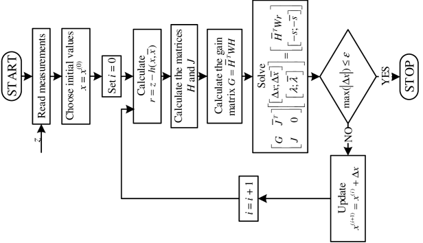
Fig. 1: Hybrid SE via Complex Equality Constrained (CEC) Normal Equations.

IV Advanced Vector Extensions: AVX-2

Modern processors support single instruction multiple data (SIMD) processor extensions, which include Advanced Vector Extensions - AVX2 [21]. AVX2 uses 256-bit registers and therefore allows the manipulation of two double precision complex values (two real and two imaginary parts) per register of CPU; this results in fast arithmetic operations with complex numbers, and makes AVX-2 ideal for implementing real-time estimation and control functions in complex variables.

Consider for illustration the product of two complex numbers:

$$\mathrm{\mathrm{\left(a1r+\mathtt{i}*a1i\right)}*\left(\mathrm{b1r+\mathtt{i}*b1i}\right)}=$$

$$\mathrm{\left(a1r*b1r-a1i*b1i\right)+\mathtt{i}*\left(a1r*b1i+a1i*b1r\right)}$$ (29)

From an implementation perspective, the non-vectorized multiplication in (29) would require 4 multiplication steps, 1 addition step, and 1 subtraction step; when performing two complex number multiplications $\left(\mathrm{a1r+\mathtt{i}*a1i}\right)*\left(\mathrm{b1r+\mathtt{i}*b1i}\right)$ and $\left(\mathrm{a2r+\mathtt{i}*a12}\mathrm{i}\right)*\left(\mathrm{b2r+\mathtt{i}*b2i}\right)$, the non-vectorized code would therefore require 8 multiplication steps, 2 addition steps, and 2 subtraction steps. In contrast, the AVX-2 code in Algorithm 1 performs the same multiplication but using 2 multiplication steps (each step involves 4 simultaneous multiplications), 1 additions/subtraction step, and 3 register shuffles. Fig. 2 illustrates the corresponding steps in the 256-bit CPU registers. In Fig. 2, $\mathrm{a}$ is a 256-bit register holding two complex numbers ($\mathrm{\left(a1r+\mathtt{i}*a1i\right)}$ and $\left(\mathrm{a2r+\mathtt{i}*a2i}\right)$), where each of the real and imaginary components are stored in a 64-bit register block; similarly, the 256-bit register $\mathrm{b}$ contains two complex numbers ($\left(\mathrm{b1r+\mathtt{i}*b1i}\right)$ and $\left(\mathrm{b2r+\mathtt{i}*b2i}\right)$). To achieve the multiplication, four intermediate results are stored in four 256-bit registers: register $\mathrm{bSwap}$ contains the swapped elements of $\mathrm{b}$, registers $\mathrm{aIm}$ and $\mathrm{aRe}$ contain only duplicates of the imaginary and real parts of $\mathrm{a}$, and the register $\mathrm{aIm}$_$\mathrm{\mathrm{b}Swap}$ holds the block register multiplication of $\mathrm{aIm}$ and $\mathrm{b}\mathrm{Swap}$. The result of the multiplication is in the register $\mathrm{res}$; it is formed using the fused multiply add/subtract function which takes the multiplication of $\mathrm{aRe}$ and $\mathrm{\mathrm{b}}$, and adds/subtracts the block registers (2 and 4)/(1 and 3) of $\mathrm{aIm}$_$\mathrm{\mathrm{b}Swap}$. The fused multiply add/subtract function is particularly targeted to complex number operations; it allows faster multiplication of two complex (double precision) numbers by two complex numbers.

AVX-2 includes several advances related to the new fused-multiply-add (FMA) instructions; these have been leveraged in the implementation of the CEC estimator in Fig. 1.

⬇

// AVX2 with fused-multiply-add intrinsics

// requires only two multiplications to multiply

// two double precision complex numbers

__m256d mult(__m256d const& a, __m256d const& b)

{

// Swap b.re and b.im

__m256d bSwap = _mm256_shuffle_pd(b,b,5);

// Imag part of a in both

__m256d aIm = _mm256_shuffle_pd(a,a,15);

// Real part of a in both

__m256d aRe = _mm256_shuffle_pd(a,a,0);

//First multiplication (a.im*b.im, a.im*b.re)

__m256d aIm_bSwap = _mm256_mul_pd(aIm, bSwap);

//Second multiplication with fused add/sub

// aRe*b + complex(-aIm_bSwap.re,aIm_bSwap.im)

return _mm256_fmaddsub_pd(aRe, b, aIm_bSwap);

}

Algorithm 1 Computation of two complex values using double precision AVX-2 with Fuse-Multiply-Add intrinsics

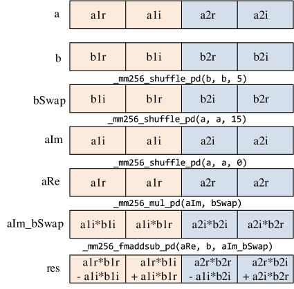
Fig. 2: Vectorized complex multiplication using AVX-2.

V Numerical Results

The CEC state estimator was programmed in C++, and the computations were performed using solvers developed via the AVX-2 processor extension [21]; comparative analysis was carried out with the CNE implementation in [19] (see section II), and with an implementation of the real variable equality constrained (REC) hybrid state estimator for handling both SCADA and PMU measurements [15]. The numerical tests were executed on a PC with an Intel i5-7600K processor and 16 GB of RAM. The termination tolerance $\varepsilon$ in Fig. 1 was set to $10^{-6}$ per-unit. The testing was carried out on the IEEE 118 test network (118), the French very high-voltage 1888 node network (1888), and part of the of the European high voltage transmission network with 9241 nodes [24]. The network information is summarized in Table II, and it includes for each network four instances of measurement placement (denoted by A, B, C, and D) with increasing number of PMU devices; columns 4 to 7 show the number of SCADA measurements, voltage PMU measurements, current PMU measurements, and zero injection measurements (when employed); the complete data sets are available for download from [25]. The corresponding percentage standard deviation of the measurements are given in Table I together with the weights. The error is simulated as Gaussian noise with zero mean and a per-unit standard deviation computed as a percentage of the meter full-scale reading. Note that the weights of the zero injection measurements are needed for the CNE estimator, but not for the CEC and REC implementations that have the zero injection measurements handled as equality constraints.

Table III shows the sparse matrix information and computational performance of CEC relative to CNE for the case without zero injection measurements, and Table IV for the case with zero injection measurements. The sparse matrix information for the CNE/CEC estimator includes the dimension of the gain/Jacobian matrix and its number of upper diagonal matrix non-zeros (NZ). For the case without zero injection measurements (Table III), the size and number of non-zeros of the CEC estimator are greater than the corresponding CNE quantities by only 1, as the only equality constraint corresponds to the slack angle equation. The CNE estimator computational results in Table III correspond to the same network and measurement sets in [19], but averaged over 200 simulations of Gaussian noise; the CEC results show a speed-up factor (SUF = time CNE/time CEC) that approaches 1.57. For the estimation results with zero injection measurements as shown in Table IV, the SUF factor also approaches a maximum value of around 1.49 with the execution times averaged over 200 trials. Note that the CEC estimator computing time on the largest instance is less than 300 ms, making it suitable for real time applications. Tables III and IV do not include a computational performance comparison with the REC method, as similar experiments reported in [19] already showed a significant computational performance advantage in favor of the CNE estimator.

Table I: Network Measurement Sets

Net.		Topology			Measurements
		#nodes	#branches		#SCADA	#V-PMU	#I-PMU	#ZeroInj
118_A		118	186		372	4	3	10
118_B		118	186		372	3	35	10
118_C		118	186		372	3	186	10
118_D		118	186		0	118	186	10
1888_A		1888	2531		5060	2	0	680
1888_B		1888	2531		5060	4	154	680
1888_C		1888	2531		5060	87	1261	680
1888_D		1888	2531		0	1888	2531	680
9241_A		9241	16049		32098	17	89	2901
9241_B		9241	16049		32098	38	2007	2901
9241_C		9241	16049		32098	66	8025	2901
9241_D		9241	16049		0	9241	16049	2901

Table II: Measurement Standard Deviations and Weights

	SCADA Measurements				PMU Measurements				ZI
	voltage	inj. power	power flows		voltage	current	ph. angle		Meas.
Std.Dev.	2%	2%	2%		0.5%	0.5%	$0.1^{\circ}$		0
Weight	1	1	1		5	5	5		25

Table III: Sparse Matrix information and Computational Performance of CNE/CEC without Zero Injection Measurements (average over 200 runs)

Net.		Matrix Size			Matrix #NZ			#Iteration			Time [ms]			SUF
		CNE	CEC		CNE	CEC		CNE	CEC		CNE	CEC
118_A		236	237		1052	1054		4.00	4.00		1.1	0.9		1.22
118_B		236	237		1052	1054		4.00	4.00		1.3	1.13		1.15
118_C		236	237		1052	1054		4.00	4.00		1.4	1.17		1.20
118_D		236	237		595	596		1.00	1.00		0.4	0.4		1.00
1888_A		3776	3777		14121	14123		5.11	5.11		26.4	23.4		1.13
1888_B		3776	3777		14121	14123		5.00	5.00		28.4	24.5		1.16
1888_C		3776	3777		14121	14123		4.00	4.00		22.3	18.1		1.23
1888_D		3776	3777		8393	8394		1.00	1.00		5.3	5.0		1.05
9241_A		18482	18483		82127	82128		5.00	5.00		312.7	189.3		1.65
9241_B		18482	18483		82127	82128		5.00	5.00		308.6	188.7		1.64
9241_C		18482	18483		82127	82128		5.00	5.00		311.4	198.8		1.57
9241_D		18482	18483		46897	46898		1.00	1.00		50.3	45.2		1.11

Table IV: Sparse Matrix information and Computational Performance of CNE/CEC with Zero Injection Measurements (average over 200 runs)

Net.		Matrix Size			Matrix #NZ			#Iteration			Time [ms]			SUF
		CNE	CEC		CNE	CEC		CNE	CEC		CNE	CEC
118_A		236	257		1146	1162		4.00	4.00		1.46	1.42		1.03
118_B		236	257		1146	1162		4.00	4.00		1.50	1.46		1.03
118_C		236	257		1146	1162		3.96	3.95		1.65	1.54		1.07
118_D		236	257		759	704		3.00	3.00		0.88	0.84		1.05
1888_A		3776	5137		20960	21106		5.00	5.00		49.17	45.53		1.08
1888_B		3776	5137		20960	21106		5.00	5.00		5.48	45.96		1.12
1888_C		3776	5137		20960	21081		5.00	5.00		55.40	47.76		1.16
1888_D		3776	5137		18971	15378		4.00	4.00		33.93	31.71		1.07
9241_A		18482	24285		100903	108594		5.00	5.00		381.85	267.30		1.43
9241_B		18482	24285		100903	108654		5.00	5.00		405.85	272.54		1.49
9241_C		18482	24285		100903	108716		5.00	5.00		412.61	283.67		1.45
9241_D		18482	24285		80116	73646		4.00	4.00		247.12	180.74		1.37

Table V: Measurement Performance Accuracy Indices with Zero Injection Measurements (average over 200 runs)

Net.	CEC	CNE	PIF-CNE	REC	PIF-REC
118_C	0.043730	0.043903	1.004	0.048352	1.106
118_D	0.006822	0.007237	1.061	0.008464	1.241
1888_C	0.180213	0.184422	1.034	0.263175	1.460
1888_D	0.002982	0.006496	2.178	0.008288	2.779
9241_C	0.133647	0.154353	1.155	0.182634	1.367
9241_D	0.001161	0.003526	3.037	0.004220	3.635

In addition to the AVX-2 CEC implementation being faster than the recent CNE implementation in [19], the CEC estimator is also more accurate than the CNE due to the exact modeling of zero injection measurements. The accuracy is quantified using performance indices for the measurement error (30) and the voltage error (31) [15]:

$$\xi_{z}=\frac{\sum_{i=1}^{m}\left|z_{i}^{estimated}-z_{i}^{true}\right|^{2}}{\sum_{i=1}^{m}\left|z_{i}^{measured}-z_{i}^{true}\right|^{2}}$$ (30)

$$\sigma_{x}^{2}=\sum_{i=\text{1}}^{n}\left|x_{i}^{estimated}-x_{i}^{true}\right|^{2}$$ (31)

For estimation with zero injection measurements, Tables V and VI respectively show the performance indices for the measurement error and voltage error. For each network in these tables, the performance indices are computed after the state vector is estimated via the CEC, the CNE [19], and the REC [15] methods. Two performance improvement factor ($\mathrm{PIF}$) ratios are used to quantify how the measurement (30) and voltage (31) performance indices of the CNE and REC estimators compare against CEC; these ratios are:

$$\mathrm{PIF{-}CNE=\frac{performance\>index\>of\>CNE}{performance\>index\>of\>CEC}}$$ (32)

$$\mathrm{PIF{-}REC=\frac{performance\>index\>of\>REC}{performance\>index\>of\>CEC}}$$ (33)

The results in Tables V and VI show that both the $\mathrm{PIF-CNE}$ and $\mathrm{PIF-REC}$ indices are consistently greater than 1, and that the performance improvement can be excess of 3 when evaluated for measurement accuracy. The CEC estimator also exhibits superior computational performance under stressed conditions leading to voltage instability [26], as evidenced by the results in Table VII; in this table, the load of the 1118_A test instance is uniformly increased and both the CEC and REC methods are used to estimate the state. At the highest load multiplication factor of 1.077, the CEC estimator required 7 iterations to converge while the REC required 10; the corresponding convergence pattern is shown in Table VIII. The CNE estimator therefore improves precision with reduced computational requirements; this makes it suitable in applications for improving the quality of state estimation [27] and enhancing the processing of bad data [28].

Table VI: Voltage Performance Accuracy Indices with Zero Injection Measurements (average over 200 runs)

Net.	CEC	CNE	PIF-CNE	REC	PIF-REC
118_C	0.000936	0.000951	1.016	0.001225	1.309
118_D	0.000074	0.000079	1.068	0.000114	1.541
1888_C	0.032794	0.033116	1.010	0.053508	1.632
1888_D	0.004831	0.005756	1.191	0.008754	1.812
9241_C	0.092998	0.099949	1.075	0.118473	1.274
9241_D	0.020224	0.022186	1.097	0.023807	1.177

Table VII: Numerical Stability Test of the CEC and REC Estimators on the 1888_A Network Instance ($\varepsilon=10^{-7}$)

Mult.		Min. Voltage			#Iter.
		Node No.	Value		CEC	REC
1.000		1194	0.83151		5	5
1.050		1194	0.81383		6	6
1.054		1194	0.81177		7	8
1.070		1194	0.80110		7	8
1.072		1194	0.79914		7	9
1.077		358	0.76614		7	10

Table VIII: Convergence Pattern of the CEC and REC Estimators on the 1888_A Network Instance with a Load Multiplier of 1.077 ($\varepsilon=10^{-7}$)

Iteration	Precision
	CEC	REC
1	1.48116e+00	1.48116e+00
2	1.19273e+00	4.22265e+00
3	5.41629e-01	6.03061e-01
4	1.71176e-01	1.37050e+00
5	1.01962e-02	1.61155e+00
6	1.45915e-04	3.87409e-01
7	1.03513e-08	5.85039e-02
8		1.33321e-03
9		2.62295e-07
10		3.20996e-13

VI Conclusion

This paper presented an algorithm for direct hybrid state estimation using a complex equality constrained normal equations approach. The complex variable formulation is advantageous for handling PMU measurements, and it is naturally suited for implementation on modern processors that allow fused multiply-accumulate operations and closely related advances. The use of equality constraints permit accurate modeling of zero injection measurements, and it has demonstrable benefits on the state estimator performance indices. The implementation of the CEC estimator is reported using the advanced vector extensions (AVX-2) set of instructions, which allows faster and specialized operations on complex numbers. Numerical results are reported on large scale transmission networks having different SCADA and PMU measurement configurations, and the results indicate that the AVX-2 implementation on networks with 9241 nodes requires less than 300 ms, thus conforming with real-time computing requirements. A comparison is carried out with two hybrid state estimation techniques: the complex normal equations (CNE) approach and the real equality constrained (REC) estimator; the comparative analysis shows that the proposed AVX-2 CEC implementation is superior to both methods in terms of solution speed and accuracy.

Complex Zero Injection Measurements

Consider the complex zero injection power at node $i$ and its conjugate:

$$s_{i} =0=u_{i}\overline{Y}_{ii}\overline{u}_{i}+u_{i}\stackrel{{\scriptstyle[}}{{\underset{}}{missing}}{k\neq i}{k=1}]{n}{\sum}\overline{Y}_{ik}\overline{u}_{k}$$ (34)

$$\overline{s}_{i} =0=\overline{u}_{i}Y_{ii}u_{i}+\overline{u}_{i}\stackrel{{\scriptstyle[}}{{\underset{}}{missing}}{k\neq i}{k=1}]{n}{\sum}Y_{ik}u_{k}$$

where

$$Y_{ii}=y_{i}^{sh}+\sum_{\underset{k\neq i}{k=1}}^{n}y_{ik},\quad Y_{ik}=-y_{ik},\quad k\neq i$$ (35)

$y_{ik}$ is the series admittance of branch $ik$, $y_{i}^{sh}$ is the shunt admittance at node $i$, $u_{i}$ is the phasor voltage at node $i$, and $n$ is the number of nodes. The corresponding elements of the Jacobian and conjugate Jacobian elements in $J$ are:

$$\frac{\partial s_{i}}{\partial u_{i}} =\overline{Y}_{ii}\overline{u}_{i}+\stackrel{{\scriptstyle[}}{{\underset{}}{missing}}{k\neq i}{k=1}]{n}{\sum}\overline{Y}_{ik}\overline{u}_{k}$$ (36)

$$\frac{\partial s_{i}}{\partial u_{k}} =0,\quad k\neq i$$

$$\frac{\partial s_{i}}{\partial\overline{u}_{i}} =\overline{Y}_{ii}u_{i}$$

$$\frac{\partial s_{i}}{\partial\overline{u}_{k}} =\overline{Y}_{ik}u_{i},\quad k\neq i$$

$$\frac{\partial\overline{s}_{i}}{\partial u_{i}} =Y_{ii}\overline{u}_{i}=\overline{\left(\frac{\partial s_{i}}{\partial\overline{u}_{i}}\right)}$$ (37)

$$\frac{\partial\overline{s}_{i}}{\partial u_{k}} =Y_{ik}\overline{u}_{i}=\overline{\left(\frac{\partial s_{i}}{\partial\overline{u}_{k}}\right)},\quad k\neq i$$

$$\frac{\partial\overline{s}_{i}}{\partial\overline{u}_{i}} =Y_{ii}u_{i}+\stackrel{{\scriptstyle[}}{{\underset{}}{missing}}{k\neq i}{k=1}]{n}{\sum}Y_{ik}u_{k}=\overline{\left(\frac{\partial s_{i}}{\partial u_{i}}\right)}$$

$$\frac{\partial\overline{s}{}_{i}}{\partial\overline{u}_{k}} =0,\quad k\neq i$$

Slack Angle

The slack angle condition requires setting the imaginary part of the slack node voltage to zero:

$$u_{s}^{im}=\frac{\mathtt{i}}{2}\left(\overline{u}_{s}-u_{s}\right)=0$$ (38)

The corresponding Jacobian and conjugate Jacobian elements in $J$ are:

$$\frac{\partial u_{s}^{im}}{\partial u_{s}} =-\frac{\mathtt{i}}{2}$$ (39)

$$\frac{\partial u_{s}^{im}}{\partial\overline{u}_{s}} =\frac{\mathtt{i}}{2}=\overline{\left(\frac{\partial u_{s}^{im}}{\partial u_{s}}\right)}$$ (40)

Izudin Džafić (M’05-SM’13) received his Ph.D. degree from University of Zagreb, Croatia in 2002. He is currently a Professor in the Department of Electrical Engineering at the International University of Sarajevo, Bosnia. From 2002 to 2014, he was with Siemens AG, Nuremberg, Germany, where he held the position of the Head of the Department and Chief Product Owner (CPO) for Distribution Network Analysis (DNA) R&D. His research interests include power system modeling, development and application of fast computing to power systems simulations. Dr. Džafić is a member of the IEEE Power and Energy Society and the IEEE Computer Society.

Rabih Jabr (M’02-SM’09-F’16) was born in Lebanon. He received the B.E. degree in electrical engineering (with high distinction) from the American University of Beirut, Beirut, Lebanon, in 1997 and the Ph.D. degree in electrical engineering from Imperial College London, London, U.K., in 2000. Currently, he is a Professor in the Department of Electrical and Computer Engineering at the American University of Beirut. His research interests are in mathematical optimization techniques and power system analysis and computing.

Bikash C. Pal (M’00-SM’02-F’13) received the B.E.E. (with honors) degree from Jadavpur University, Calcutta, India, the M.E. degree from the Indian Institute of Science, Bangalore, India, and the Ph.D. degree from Imperial College London, London, U.K., in 1990, 1992, and 1999, respectively, all in electrical engineering. Currently, he is a Professor in the Department of Electrical and Electronic Engineering, Imperial College London. His current research interests include state estimation, power system dynamics, and flexible ac transmission system controllers.

References

[1]
R. R. Nucera and M. L. Gilles, “A blocked sparse matrix formulation for the
solution of equality-constrained state estimation,” IEEE Trans. on
Power Syst., vol. 6, no. 1, pp. 214–224, Feb. 1991.
[2]
A. Abur and A. Gómez Expósito, Power System State Estimation:
Theory and Implementation. New York,
NY: Marcel Dekker, 2004.
[3]
C. Gómez-Quiles, H. A. Gil, A. de la Villa Jaén, and
A. Gómez-Expósito, “Equality-constrained bilinear state
estimation,” IEEE Trans. Power Syst., vol. 28, no. 2, pp. 902–910,
May 2013.
[4]
A. F. Taha, J. Qi, J. Wang, and J. H. Panchal, “Risk mitigation for dynamic
state estimation against cyber attacks and unknown inputs,” IEEE
Trans. Smart Grid, vol. 9, no. 2, pp. 886–899, Mar. 2018.
[5]
A. Borghetti, R. Bottura, M. Barbiroli, and C. A. Nucci, “Synchrophasors-based
distributed secondary voltage/var control via cellular network,” IEEE
Trans. Smart Grid, vol. 8, no. 1, pp. 262–274, Jan. 2017.
[6]
C. Xu and A. Abur, “A fast and robust linear state estimator for very large
scale interconnected power grids,” IEEE Trans. Smart Grid - Early
Access, 2017.
[7]
M. Zhou, V. A. Centeno, J. S. Thorp, and A. G. Phadke, “An alternative for
including phasor measurements in state estimators,” IEEE Trans. Power
Syst., vol. 21, no. 4, pp. 1930–1937, Nov. 2006.
[8]
R. F. Nuqui and A. G. Phadke, “Hybrid linear state estimation utilizing
synchronized phasor measurements,” in 2007 IEEE Lausanne Power Tech.,
Jul. 2007, pp. 1665–1669.
[9]
Y. Cheng, X. Hu, and B. Gou, “A new state estimation using synchronized phasor
measurements,” in 2008 IEEE International Symposium on Circuits and
Systems, May 2008, pp. 2817–2820.
[10]
R. Baltensperger, A. Loosli, H. Sauvain, M. Zima, G. Andersson, and R. Nuqui,
“An implementation of two-stage hybrid state estimation with limited number
of PMU,” in 10th IET International Conference on Developments in
Power System Protection (DPSP 2010), Mar. 2010, pp. 1–5.
[11]
A. Simões Costa, A. Albuquerque, and D. Bez, “An estimation fusion method
for including phasor measurements into power system real-time modeling,”
IEEE Trans. Power Syst., vol. 28, no. 2, pp. 1910–1920, May 2013.
[12]
T. Wu, C. Y. Chung, and I. Kamwa, “A fast state estimator for systems
including limited number of PMUs,” IEEE Trans. Power Syst.,
vol. 32, no. 6, pp. 4329–4339, Nov. 2017.
[13]
T. Bi, X. Qin, and Q. Yang, “A novel hybrid state estimator for including
synchronized phasor measurements,” Elec. Power Syst. Res., vol. 78,
no. 8, pp. 1343–1352, Aug. 2008.
[14]
S. Chakrabarti, E. Kyriakides, G. Ledwich, and A. Ghosh, “Inclusion of PMU
current phasor measurements in a power system state estimator,” IET
Gener. Transm. Distrib., vol. 4, no. 10, pp. 1104–1115, Oct. 2010.
[15]
G. Valverde, S. Chakrabarti, E. Kyriakides, and V. Terzija, “A constrained
formulation for hybrid state estimation,” IEEE Trans. Power Syst.,
vol. 26, no. 3, pp. 1102–1109, Aug. 2011.
[16]
V. Murugesan, Y. Chakhchoukh, V. Vittal, G. T. Heydt, N. Logic, and
S. Sturgill, “PMU data buffering for power system state estimators,”
IEEE Power and Energy Tech. Syst. J., vol. 2, no. 3, pp. 94–102, Sep.
2015.
[17]
M. Glavic and T. Van Cutsem, “Reconstructing and tracking network state from
a limited number of synchrophasor measurements,” IEEE Trans. Power
Syst., vol. 28, no. 2, pp. 1921–1929, May 2013.
[18]
M. Göl and A. Abur, “A hybrid state estimator for systems with limited
number of PMUs,” IEEE Trans. Power Syst., vol. 30, no. 3, pp.
1511–1517, May 2015.
[19]
I. Džafić, R. A. Jabr, and T. Hrnjić, “Hybrid state estimation in
complex variables,” IEEE Trans. on Power Syst. - Early Access, 2018.
[20]
C. J. Hughes, Single-Instruction Multiple-Data Execution. Morgan & Claypool, 2015. [Online]. Available:
http://ieeexplore.ieee.org/xpl/articleDetails.jsp?arnumber=7123244
[21]
C. Lomont, “Introduction to Intel advanced vector extensions,”
https://software.intel.com/en-us/articles/introduction-to-intel-advanced-vector-extensions,
Jun. 2011, accessed: 2018-06-3.
[22]
W. Wirtinger, “Zur formalen theorie der funktionen von mehr komplexen
veranderlichen,” Mathematische Annalen, vol. 97, pp. 257–376, 1927.
[23]
K. Kreutz-Delgado, “The complex gradient operator and the CR-calculus,”
ArXiv e-prints, arXiv:0906.4835v1, 2009.
[24]
C. Josz, S. Fliscounakis, J. Maeght, and P. Panciatici, “AC power flow data
in MATPOWER and QCQP format: iTesla, RTE snapshots, and PEGASE,”
ArXiv e-prints, arXiv:1603.01533, 2016.
[25]
I. Džafić, R. A. Jabr, and B. C. Pal, “Vector implementation of
equality-constrained hybrid state estimation in complex variables - test
networks,”
https://www.dropbox.com/s/1pl5itl2v43juw6/SE_TestNetworks.7z?dl=1,
accessed: 2018-6-5.
[26]
V. A. Venikov, V. A. Stroev, V. I. Idelchick, and V. I. Tarasov, “Estimation
of electrical power system steady-state stability in load flow
calculations,” IEEE Trans. Power Appar. Syst., vol. 94, no. 3, pp.
1034–1041, May 1975.
[27]
E. W. S. Ângelos and E. N. Asada, “Improving state estimation with real-time
external equivalents,” IEEE Trans. Power Syst., vol. 31, no. 2, pp.
1289–1296, Mar. 2016.
[28]
M. B. Do Coutto Filho, J. C. S. de Souza, and M. A. Ribeiro Guimaraens,
“Enhanced bad data processing by phasor-aided state estimation,” IEEE
Trans. Power Syst., vol. 29, no. 5, pp. 2200–2209, Sep. 2014.