The calculation of differential and total cross sections for $W^{+}W^{-}\gamma$ production process in proton-proton collisions at LHC energies

Abstract

The vector bosons production at the Large Hadron Collider makes it possible to investigate in detail the basic structure of electroweak interactions. Besides the LHC with a good accuracy will be measure production of weak bosons ($pp\to W^{+}W^{-}$). The production of weak bosons with photon ($pp\to W^{+}W^{-}\gamma$) provides an increasingly powerful handle at higher center-of-mass energies.
We present phenomenological results for $WW\gamma$ production in proton-proton interaction at the Large Hadron Collider. In this paper, we calculate the total and differential cross sections. We consider the dependence of differential cross section distributions on transverse momentum and rapidity particles, which are produced in the final state ($W^{+}$ and $W^{-}$). We consider several important distributions, which are included in the search for new physics at the Large Hadron Collider.
The results for transverse momentum distributions, rapidity distributions and total cross section are presented.

I Introduction

The fundamental description of matter and the forces that determine its behavior are constantly studied in particle physics.
The new physics, which underlies the dynamics of the electroweak symmetry breaking is one of the outstanding open questions of the Standard Model.
Massive vector boson production is among the most important electroweak processes at hadron colliders. This makes is it possible to study in detail the structure of the gauge symmetry of electroweak interactions and the electroweak symmetry breaking mechanism.
At Tevatron and the LHC, various measurements of the $W^{+}W^{-}$ production have been carried out I1 ; I2 ; II1 ; II2 ; II3 ; II4 ; II5 ; I3 ; IC1 ; IC2 ; IC3 ; IC4 ; I4 ; I5 ; I6 and it was shown that the total $W^{+}W^{-}$ cross section at 8 $TeV$ and 13 $TeV$ exceeds theoretical expectations and causes possible phenomena of new physics I71 ; I72 ; I7 ; I8 ; I9 ; I10 ; I11 ; I12 ; I13 .
The vector-bosons production plays an important role in various areas of the Large Hadron Collider (LHC) physics programme. Experimental studies of these processes permit one to test key aspects of the Standard Model (SM) at energies up to the TeV regime.

It should be noted that precise calculations of vector-bosons production have reached a new era with the recent results at the next-to-next-to-leading order (NNLO) QCD precision for V + 1 jet L1 as well as have been used to precisely describe backgrounds for dark matter searches L2 .
In recent years, owing to the Large Hadron Collider (LHC), particle physicists at CERN have gained access to more accurate testing of the parameters of the Standard Model.
Therefore, we want to consider an important SM process of the vector boson production in proton-proton collisions at LHC energy.
At leading order of perturbation theory, we will consider the $W^{+}W^{-}\gamma$ production described by one of the subprocesses, namely, quark-antiquark scattering.
At present, one of the prime targets for experiments is the measurement of the $WW\gamma$ and $WWZ$ couplings. In the Standard Model these couplings are unambiguously fixed by the non-abelian nature of the SU (2) $\times$ U (1) gauge symmetry.

The underlying theory of our calculations is the SM of particle physics. Since we deal with the production of weak bosons, we will take into account the electroweak sector, too.
One of the functions that describes the interaction of partons in a hadron is the distribution of the dependence on the transverse momentum. The transverse momentum dependent distributions naturally appear within factorization theorem for the differential cross section of inclusive hard processes Col1 ; Col2 .
The Large Hadron Collider (LHC) at CERN allows the vector boson production with transverse momenta in the TeV regime in proton-proton collisions (pp) with a centre-of-mass energy of $\sqrt{s}=7\,\,{\mbox{or}}\,\,8\,\,{\mbox{or}}\,\,14\,\,TeV$.
The production $WW\gamma$ and $WZ\gamma$ of triboson has been studied from proton-proton collisions at a centre-of-mass energy of $\sqrt{s}=8\,\,TeV$ recorded with the ATLAS detector corresponding to an integrated luminosity of 20.2 $fb^{-1}$ ATLAS , and the CMS detector data correspond to an integrated luminosity of 19.3 $fb^{-1}$ CMS at the LHC.
The $WW\gamma$ production in the proton-proton collision is analyzed in the Sokolenko , and it is shown that this channel can discover new physics at the LHC.
In some works Y ; J ; B using ATLAS and CMS data, the di- and multiboson $(ZZ,WZ,WW,WW\gamma\,\,\,{\rm and}\,\,\,WZ\gamma)$ productions $pp$ collisions at $\sqrt{s}=8\,\,\,{\rm and}\,\,\,13\,\,TeV$ are studied.
The detailed theoretical investigation was carried out of the $WW,WZ,ZZ,W\gamma,Z\gamma$ vector bosons production and $WWg,ZZg,ZZq$ productions in the process of $pp$ collisions WW1 ; WW2 ; WW3 ; WW4 ; WW41 ; WW42 . In WW5 , was theoretically investigated the production of $W^{+}W^{-}\gamma$ in the process of $pp$ collisions.
It should be noted that the study of the $W^{+}W^{-}\gamma$ production process may be will be for the good perform of accurate tests of the description of electroweak and strong interactions in the standard model (SM).
The Standard Model of particle physics describes most of high-energy experimental data. In SM1 , the cross-section of the $WW$ and $WZ$ production has been precisely measured at the LHC and found to be in agreement with the SM expectation. By extending the analysis of the inclusive $WW+WZ$ diboson production cross section in proton-proton collisions, the production of three gauge bosons $WW(WZ)\gamma$ SM2 was observed.
It can be predicted that the $WW\gamma$ production also provides a potential background for new physics searches, such as supersymmetric particles.
There is great interest in the two and three gauge-boson production of final states in proton-proton interaction at high-energy colliders, since they will allow crucial tests of the electroweak gauge theory.
Taking into account the above, one can come to the conclusion that the study of the $WW\gamma$ production in proton-proton collisions presents the most interesting problems for LHC and other colliders.
Thus, in the present paper we will investigate these problems; i.e. considering the LHC conditions, we will calculate cross sections of the $WW\gamma$ production in proton-proton collisions.

We can write convolution of the matrix element of process and the universal parton density functions for obtaining an inclusive cross section for a given scattering process with the use of the factorization theorem in perturbative quantum chromodynamics (pQCD).
We present the cross sections for the vector boson production to study the effect of contributions separating single boson and diboson production.

II General framework

In this section we want to discuss the $WW\gamma$ three bosons production in hadron-hadron collisions at LHC energy.
The process is written in the form

$$p(P_{1})+p(P_{2})\to W^{-}(k_{1})+W^{+}(k_{2})+\gamma(k_{3}).$$ (1)

The $W^{+}W^{-}\gamma$ production at the LHC is obtained form the quark-antiquark annihilation subprocess at the parton level:

$$q(p_{1})+\bar{q}(p_{2})\to W^{-}(k_{1})+W^{+}(k_{2})+\gamma(k_{3}).$$ (2)

To calculate the cross section, we need to consider all diagrams. In this process, we have fifteen Feynman diagrams.
The leading order (LO) of all Feynman diagrams for (2) process is illustrated in Figs.1, 2 and 3, respectively.

Figure 1: The Feynman diagrams for the process $q\bar{q}\to W^{+}W^{-}\gamma$.

Figure 2: The Feynman diagrams for the process $q\bar{q}\to W^{+}W^{-}\gamma$.

Figure 3: The Feynman diagrams for the process $q\bar{q}\to W^{+}W^{-}\gamma$.

The general couplings of two charged vector bosons with a neutral vector boson, $WW\gamma$ and $WWZ$, can be derived from the following effective Lagrangian, which conserves $C$ (charge) and $P$ (parity) separately, can be given as follows L3 ; L4 ; L5 :

$${\mathcal{L}} = ig_{WW\gamma}[g_{1}^{\gamma}(W_{\mu\nu}^{\dagger}W^{\mu}A^{\nu}-W^{\mu\nu}W_{\mu}^{\dagger}A_{\nu})+\kappa_{\gamma}W_{\mu}^{\dagger}W_{\nu}A^{\mu\nu}+\frac{\lambda_{\gamma}}{m_{W}^{2}}W_{\rho\mu}^{\dagger}W_{\nu}^{\mu}A^{\nu\rho}]$$ (3)

$$+ ig_{WWZ}[g_{1}^{Z}(W_{\mu\nu}^{\dagger}W^{\mu}Z^{\nu}-W^{\mu\nu}W_{\mu}^{\dagger}Z_{\nu})+\kappa_{Z}W_{\mu}^{\dagger}W_{\nu}Z^{\mu\nu}+\frac{\lambda_{Z}}{m_{W}^{2}}W_{\rho\mu}^{\dagger}W_{\nu}^{\mu}Z^{\nu\rho}],$$

where $X_{\mu\nu}\equiv\partial_{\mu}X_{\nu}-\partial_{\nu}X_{\mu}$ $(X_{\mu}=W_{\mu},A_{\mu},Z_{\mu}$) and the coefficients $g^{\gamma,Z}_{1}$, $k_{\gamma,Z}$ and $\lambda_{\gamma,Z}$ are defined to be $g^{\gamma,Z}_{1}=k_{\gamma,Z}=1$ and $\lambda_{\gamma,Z}=0$ in the Standard Model, and the overall coupling constants $g_{WWV}$ are given by $g_{WW\gamma}=-e$ and $g_{WWZ}=-e\cot\theta_{W}$, respectively, with $\theta_{W}$ being the weak mixing angle and $e$ being the positron charge.
It should be noted that triple gauge couplings were thoroughly measured at LEP2 LEP .
For the W W interaction, many phenomenological processes at linear and hadron colliders were studied LW1 ; LW2 ; LW3 ; LW4 ; LW5 ; LW6 ; LW7 ; LW8 ; LW9 ; LW10 .

We can write the Feynman amplitudes for the partonic process $q+\bar{q}\to W^{-}+W^{+}+\gamma$ as

$$M_{1} = -K_{1}\cdot\bar{v}(p_{2},m_{q})\cdot\gamma_{\mu}\cdot u(p_{1},m_{q})\cdot\biggl{[}(k_{2}-k_{3})^{\rho}g_{\beta\nu}+(-2k_{2}-k_{3})^{\nu}g_{\beta\rho}+(k_{2}+2k_{3})^{\beta}g_{\nu\rho}\biggr{]}\cdot$$

$$\cdot g_{\mu\sigma}\cdot\biggl{[}(2k_{1}+k_{2}+k_{3})^{\lambda}g_{\alpha\sigma}+(k_{2}+k_{3}-k_{1})^{\sigma}g_{\alpha\lambda}+(-k_{1}-2k_{2}-2k_{3})^{\alpha}g_{\sigma\lambda}\biggr{]}\cdot$$

$$\cdot g_{\rho\lambda}\cdot\frac{1}{(k_{2}+k_{3})^{2}-M^{2}_{W}+iM_{W}\Gamma_{W}}\cdot\frac{1}{(k_{1}+k_{2}+k_{3})^{2}}\cdot\varepsilon^{\ast}_{\nu}(k_{3})\varepsilon^{\ast}_{\alpha}(k_{1})\varepsilon^{\ast}_{\beta}(k_{2});$$

$$M_{2} = K_{2}\cdot\bar{v}(p_{2},m_{q})\cdot\gamma_{\mu}\cdot u(p_{1},m_{q})\cdot\biggl{[}(k_{2}-k_{3})^{\rho}g_{\beta\nu}+(-2k_{2}-k_{3})^{\nu}g_{\beta\rho}+(k_{2}+2k_{3})^{\beta}g_{\nu\rho}\biggr{]}\cdot$$

$$\cdot g_{\mu\sigma}\cdot\biggl{[}(2k_{1}+k_{2}+k_{3})^{\lambda}g_{\alpha\sigma}+(k_{2}+k_{3}-k_{1})^{\sigma}g_{\alpha\lambda}+(-k_{1}-2k_{2}-2k_{3})^{\alpha}g_{\sigma\lambda}\biggr{]}\cdot$$

$$\cdot g_{\rho\lambda}\cdot\frac{1}{(k_{2}+k_{3})^{2}-M^{2}_{W}+iM_{W}\Gamma_{W}}\cdot\frac{1}{(k_{1}+k_{2}+k_{3})^{2}-M^{2}_{Z}+iM_{Z}\Gamma_{Z}}\cdot\varepsilon^{\ast}_{\nu}(k_{3})\varepsilon^{\ast}_{\alpha}(k_{1})\varepsilon^{\ast}_{\beta}(k_{2});$$

$$M_{3} = -K_{3}\cdot\bar{v}(p_{2},m_{q})\cdot\gamma_{\mu}(\hat{k}_{1}-\hat{p}_{2}+m_{q})\gamma_{\nu}(\hat{k}_{1}+\hat{k}_{2}-\hat{p}_{2}+m_{q})\gamma_{\rho}\cdot u(p_{1},m_{q})\cdot$$

$$\cdot\frac{1}{(p_{2}-k_{1})^{2}-m^{2}_{q}}\cdot\frac{1}{(p_{2}-k_{1}-k_{2})^{2}-m^{2}_{q}}\cdot\varepsilon^{\ast}_{\rho}(k_{3})\varepsilon^{\ast}_{\mu}(k_{1})\varepsilon^{\ast}_{\nu}(k_{2});$$

$$M_{4} = -K_{4}\cdot\bar{v}(p_{2},m_{q})\cdot\gamma_{\mu}(\hat{k}_{1}-\hat{p}_{2}+m_{q})\gamma_{\nu}\cdot u(p_{1},m_{q})\cdot\biggl{[}(k_{2}-k_{3})^{\rho}g_{\sigma\alpha}+(-2k_{2}-k_{3})^{\alpha}g_{\sigma\rho}+$$

$$+(k_{2}+2k_{3})^{\sigma}g_{\rho\alpha}\biggr{]}g_{\nu\rho}\cdot\frac{1}{(p_{2}-k_{1})^{2}-m^{2}_{q}}\cdot\frac{1}{(k_{2}+k_{3})^{2}-M^{2}_{W}+iM_{W}\Gamma_{W}}\cdot\varepsilon^{\ast}_{\alpha}(k_{3})\varepsilon^{\ast}_{\mu}(k_{1})\varepsilon^{\ast}_{\sigma}(k_{2});$$

$$M_{5} = -K_{5}\cdot\bar{v}(p_{2},m_{q})\cdot\gamma_{\mu}(\hat{k}_{3}-\hat{p}_{2}+m_{q})\gamma_{\nu}(\hat{k}_{1}+\hat{k}_{3}-\hat{p}_{2}+m_{q})\gamma_{\rho}\cdot u(p_{1},m_{q})\cdot$$

$$\cdot\frac{1}{(p_{2}-k_{3})^{2}-m^{2}_{q}}\cdot\frac{1}{(p_{2}-k_{1}-k_{3})^{2}-m^{2}_{q}}\cdot\varepsilon^{\ast}_{\mu}(k_{3})\varepsilon^{\ast}_{\nu}(k_{1})\varepsilon^{\ast}_{\rho}(k_{2});$$

$$M_{6} = K_{6}\cdot\bar{v}(p_{2},m_{q})\cdot\gamma_{\mu}\cdot u(p_{1},m_{q})\cdot g_{\mu\sigma}\cdot\frac{1}{(k_{1}+k_{2}+k_{3})^{2}}\cdot\varepsilon^{\ast}_{\alpha}(k_{1})\varepsilon^{\ast}_{\beta}(k_{2})\varepsilon^{\ast}_{\nu}(k_{3})\cdot$$

$$\cdot[g_{\alpha\sigma}g_{\beta\nu}+g_{\alpha\nu}g_{\beta\sigma}-2g_{\alpha\beta}g_{\nu\sigma}];$$

$$M_{7} = -K_{7}\cdot\bar{v}(p_{2},m_{q})\cdot\gamma_{\mu}\cdot u(p_{1},m_{q})\cdot g_{\mu\sigma}\frac{1}{(k_{1}+k_{2}+k_{3})^{2}-M^{2}_{Z}+iM_{Z}\Gamma_{Z}}\cdot$$

$$\cdot\varepsilon^{\ast}_{\alpha}(k_{1})\varepsilon^{\ast}_{\beta}(k_{2})\varepsilon^{\ast}_{\nu}(k_{3})\cdot\biggl{[}-g_{\alpha\sigma}g_{\beta\nu}-g_{\alpha\nu}g_{\beta\sigma}+2g_{\alpha\beta}g_{\nu\sigma}\biggr{]};$$

$$M_{8} = K_{8}\cdot\bar{v}(p_{2},m_{q})\cdot\gamma_{\mu}\cdot u(p_{1},m_{q})\cdot\biggl{[}(k_{1}-k_{3})^{\rho}g_{\alpha\nu}+(-2k_{1}-k_{3})^{\nu}g_{\alpha\rho}+(k_{1}+2k_{3})^{\alpha}g_{\nu\rho}\biggr{]}g_{\mu\sigma}\cdot$$

$$\cdot\biggl{[}(k_{1}+2k_{2}+k_{3})^{\lambda}g_{\beta\sigma}+(k_{1}-k_{2}+k_{3})^{\sigma}g_{\beta\lambda}+(-2k_{1}-k_{2}-2k_{3})^{\beta}g_{\sigma\lambda}\biggr{]}g_{\rho\lambda}\cdot$$

$$\cdot\frac{1}{(k_{1}+k_{3})^{2}-M^{2}_{W}+iM_{W}\Gamma_{W}}\cdot\frac{1}{(k_{1}+k_{2}+k_{3})^{2}}\cdot\varepsilon^{\ast}_{\nu}(k_{3})\varepsilon^{\ast}_{\alpha}(k_{1})\varepsilon^{\ast}_{\beta}(k_{2});$$

$$M_{9} = K_{9}\cdot\bar{v}(p_{2},m_{q})\cdot\gamma_{\mu}\cdot u(p_{1},m_{q})\cdot\biggl{[}(k_{1}-k_{3})^{\rho}g_{\alpha\nu}+(-2k_{1}-k_{3})^{\nu}g_{\alpha\rho}+(k_{1}+2k_{3})^{\alpha}g_{\nu\rho}\biggr{]}g_{\mu\sigma}\cdot$$

$$\cdot\biggl{[}(k_{1}+2k_{2}+k_{3})^{\lambda}g_{\beta\sigma}+(k_{1}-k_{2}+k_{3})^{\sigma}g_{\beta\lambda}+(-2k_{1}-k_{2}-2k_{3})^{\beta}g_{\sigma\lambda}\biggr{]}g_{\rho\lambda}\cdot$$

$$\cdot\frac{1}{(k_{1}+k_{3})^{2}-M^{2}_{W}+iM_{W}\Gamma_{W}}\cdot\frac{1}{(k_{1}+k_{2}+k_{3})^{2}-M^{2}_{Z}+iM_{Z}\Gamma_{Z}}\cdot\varepsilon^{\ast}_{\nu}(k_{3})\varepsilon^{\ast}_{\alpha}(k_{1})\varepsilon^{\ast}_{\beta}(k_{2});$$

$$M_{10} = -K_{10}\cdot\bar{v}(p_{2},m_{q})\cdot\gamma_{\mu}(\hat{k}_{1}+\hat{k}_{3}-\hat{p}_{2}+m_{q})\gamma_{\nu}\cdot u(p_{1},m_{q})\cdot\biggl{[}(k_{1}-k_{3})^{\alpha}g_{\sigma\rho}+(-2k_{1}-k_{3})^{\sigma}g_{\alpha\rho}+$$

$$+(k_{1}+2k_{3})^{\rho}g_{\sigma\alpha}\biggr{]}g_{\nu\alpha}\cdot\frac{1}{(p_{2}-k_{1}-k_{3})^{2}-m^{2}_{q}}\cdot\frac{1}{(k_{1}+k_{3})^{2}-M^{2}_{W}+iM_{W}\Gamma_{W}}\cdot$$

$$\cdot\varepsilon^{\ast}_{\sigma}(k_{3})\varepsilon^{\ast}_{\rho}(k_{1})\varepsilon^{\ast}_{\nu}(k_{2});$$

$$M_{11} = -K_{11}\cdot\bar{v}(p_{2},m_{q})\cdot\gamma_{\mu}(\hat{k}_{1}+\hat{k}_{2}-\hat{p}_{2}+m_{q})\gamma_{\nu}\cdot u(p_{1},m_{q})\cdot\biggl{[}(k_{1}-k_{2})^{\sigma}g_{\alpha\beta}+(-2k_{1}-k_{2})^{\beta}g_{\alpha\sigma}+$$

$$+(k_{1}+2k_{2})^{\alpha}g_{\beta\sigma}\biggr{]}g_{\mu\sigma}\cdot\frac{1}{(p_{2}-k_{1}-k_{2})^{2}-m^{2}_{q}}\cdot\frac{1}{(k_{1}+k_{2})^{2}}\cdot\varepsilon^{\ast}_{\nu}(k_{3})\varepsilon^{\ast}_{\alpha}(k_{1})\varepsilon^{\ast}_{\beta}(k_{2});$$

$$M_{12} = K_{12}\cdot\bar{v}(p_{2},m_{q})\cdot\gamma_{\mu}(\hat{k}_{1}+\hat{k}_{2}-\hat{p}_{2}+m_{q})\gamma_{\nu}\cdot u(p_{1},m_{q})\cdot\biggl{[}(k_{1}-k_{2})^{\sigma}g_{\alpha\beta}+(-2k_{1}-k_{2})^{\beta}g_{\alpha\sigma}+$$

$$+(k_{1}+2k_{2})^{\alpha}g_{\beta\sigma}\biggr{]}g_{\mu\sigma}\cdot\frac{1}{(p_{2}-k_{1}-k_{2})^{2}-m^{2}_{q}}\cdot\frac{1}{(k_{1}+k_{2})^{2}-M^{2}_{Z}+iM_{Z}\Gamma_{Z}}\cdot\varepsilon^{\ast}_{\nu}(k_{3})\varepsilon^{\ast}_{\alpha}(k_{1})\varepsilon^{\ast}_{\beta}(k_{2});$$

$$M_{13} = K_{13}\cdot\bar{v}(p_{2},m_{q})\cdot\gamma_{\mu}(\hat{k}_{3}-\hat{p}_{2}+m_{q})\gamma_{\nu}\cdot u(p_{1},m_{q})\cdot\biggl{[}(k_{1}-k_{2})^{\sigma}g_{\alpha\beta}+(-2k_{1}-k_{2})^{\beta}g_{\alpha\sigma}+$$

$$+(k_{1}+2k_{2})^{\alpha}g_{\beta\sigma}\biggr{]}g_{\nu\sigma}\cdot\frac{1}{(p_{2}-k_{3})^{2}-m^{2}_{q}}\cdot\frac{1}{(k_{1}+k_{2})^{2}}\cdot\varepsilon^{\ast}_{\mu}(k_{3})\varepsilon^{\ast}_{\alpha}(k_{1})\varepsilon^{\ast}_{\beta}(k_{2});$$

$$M_{14} = K_{14}\cdot\bar{v}(p_{2},m_{q})\cdot\gamma_{\mu}(\hat{k}_{3}-\hat{p}_{2}+m_{q})\gamma_{\nu}\cdot u(p_{1},m_{q})\cdot\biggl{[}(k_{1}-k_{2})^{\sigma}g_{\alpha\beta}+(-2k_{1}-k_{2})^{\beta}g_{\alpha\sigma}+$$

$$+(k_{1}+2k_{2})^{\alpha}g_{\beta\sigma}\biggr{]}g_{\nu\sigma}\cdot\frac{1}{(p_{2}-k_{3})^{2}-m^{2}_{q}}\cdot\frac{1}{(k_{1}+k_{2})^{2}-M^{2}_{Z}+iM_{Z}\Gamma_{Z}}\cdot\varepsilon^{\ast}_{\mu}(k_{3})\varepsilon^{\ast}_{\alpha}(k_{1})\varepsilon^{\ast}_{\beta}(k_{2});$$

$$M_{15} = K_{15}\cdot\bar{v}(p_{2},m_{q})\cdot\gamma_{\mu}(\hat{k}_{1}-\hat{p}_{2}+m_{q})\gamma_{\nu}(\hat{k}_{1}+\hat{k}_{3}-\hat{p}_{2}+m_{q})\gamma_{\rho}\cdot u(p_{1},m_{q})\cdot$$ (4)

$$\cdot\frac{1}{(p_{2}-k_{1})^{2}-m^{2}_{q}}\cdot\frac{1}{(p_{2}-k_{1}-k_{3})^{2}-m^{2}_{q}}\cdot\varepsilon^{\ast}_{\nu}(k_{3})\varepsilon^{\ast}_{\mu}(k_{1})\varepsilon^{\ast}_{\rho}(k_{2});$$

here $M_{W}$, $M_{Z}$, $\Gamma_{W}$ and $\Gamma_{Z}$ are the masses and the decay width of the $W$ and $Z$ bosons, respectively. $p_{1}$ and $p_{2}$ are the 4-momenta of the quark and anti-quark in the initial state. $\varepsilon_{\mu}(k_{1}),\,\,\,\varepsilon_{\nu}(k_{2})$ are the polarization vectors of $W^{-},\,\,W^{+}$ bosons, and $\varepsilon_{\rho}(k_{3})$ is the polarization vector of the photon, $k_{1},\,\,\,k_{2}$, and $k_{3}$ are 4-momenta of $W^{-},\,\,W^{+}$, and photon, respectively.
$K_{1},K_{2},K_{3},K_{4},K_{5},K_{6},K_{7},K_{8},K_{9},K_{10},K_{11},K_{12},K_{13},K_{14},K_{15}$ are the coefficients that are obtained from the Feynman rule for every amplitude of the diagrams, respectively.

$$K_{1}=\frac{4e^{3}}{3};\,\,\,\,K_{2}=e^{3}\cdot\frac{Cos\theta_{W}}{Sin\theta_{W}}\cdot\biggl{[}\frac{\frac{1}{2}-\frac{2Sin^{2}\theta_{W}}{3}}{Cos\theta_{W}Sin\theta_{W}}-\frac{2Sin\theta_{W}}{3Cos\theta_{W}}\biggr{]};\,\,\,\,K_{3}=\frac{16e}{3}M^{2}_{W}\frac{G_{F}}{\sqrt{2}}|V_{ud}|^{2};$$

$$K_{4}=4eM^{2}_{W}\frac{G_{F}}{\sqrt{2}}|V_{ud}|^{2};\,\,\,\,K_{5}=\frac{16e}{3}M^{2}_{W}\frac{G_{F}}{\sqrt{2}}|V_{ud}|^{2};\,\,\,\,K_{6}=\frac{4e^{3}}{3};$$

$$K_{7}=e^{3}\frac{Cos\theta_{W}}{Sin\theta_{W}}\cdot\biggl{[}\frac{\frac{1}{2}-\frac{2Sin^{2}\theta_{W}}{3}}{Cos\theta_{W}Sin\theta_{W}}-\frac{2Sin\theta_{W}}{3Cos\theta_{W}}\biggr{]};\,\,\,\,K_{8}=\frac{4e^{3}}{3};$$

$$K_{9}=e^{3}\frac{Cos\theta_{W}}{Sin\theta_{W}}\cdot\biggl{[}\frac{\frac{1}{2}-\frac{2Sin^{2}\theta_{W}}{3}}{Cos\theta_{W}Sin\theta_{W}}-\frac{2Sin\theta_{W}}{3Cos\theta_{W}}\biggr{]};\,\,\,\,K_{10}=4eM^{2}_{W}\frac{G_{F}}{\sqrt{2}}|V_{ud}|^{2};\,\,\,\,K_{11}=\frac{16e^{3}}{9};$$

$$K_{12}=\frac{4e^{3}}{3}\cdot\frac{Cos\theta_{W}}{Sin\theta_{W}}\cdot\biggl{[}\frac{\frac{1}{2}-\frac{2Sin^{2}\theta_{W}}{3}}{Cos\theta_{W}Sin\theta_{W}}-\frac{2Sin\theta_{W}}{3Cos\theta_{W}}\biggr{]};\,\,\,\,K_{13}=\frac{16e^{3}}{9};$$

$$K_{14}=\frac{4e^{3}}{3}\cdot\frac{Cos\theta_{W}}{Sin\theta_{W}}\cdot\biggl{[}\frac{\frac{1}{2}-\frac{2Sin^{2}\theta_{W}}{3}}{Cos\theta_{W}Sin\theta_{W}}-\frac{2Sin\theta_{W}}{3Cos\theta_{W}}\biggr{]};\,\,\,\,K_{15}=\frac{8e}{3}M^{2}_{W}\frac{G_{F}}{\sqrt{2}}|V_{ud}|^{2}.$$ (5)

where the quantities $M_{W}$, $e=\sqrt{4\pi\alpha}$, $G_{F}$, $V_{ud}$, and $\theta_{W}$ are the W-boson mass, the elementary electric charge ($\alpha\sim 1/137$), the Fermi coupling constant, one of the elements of the Cabibbo - Kobayashi - Maskawa matrix, and the weak mixing angle, respectively.
Full square matrix element can be written as follows

$$\overline{|{\mathcal{M}}|^{2}}=\sum|M_{1}+M_{2}+M_{3}+M_{4}+M_{5}+M_{6}+M_{7}+M_{8}+M_{9}+$$

$$+M_{10}+M_{11}+M_{12}+M_{13}+M_{14}+M_{15}|^{2}.$$ (6)

II.1 The kinematics

For the subprocesses (2) Mandelstam invariants we can be written in the following form:

$$s=(p_{1}+p_{2})^{2}=(k_{1}+k_{2}+k_{3})^{2};\,\,\,t=(p_{1}-k_{3})^{2}=(k_{1}+k_{2}-p_{2})^{2};$$

$$u=(p_{2}-k_{3})^{2}=(k_{1}+k_{2}-p_{1})^{2};\,\,\,q_{1}=(p_{1}-k_{1})^{2}=(k_{2}+k_{3}-p_{2})^{2};$$

$$q_{2}=(p_{2}-k_{2})^{2}=(k_{1}+k_{3}-p_{1})^{2}.$$ (7)

We can define five additional invariant parameters, which will be expressed through the main invariant variables (2):

$$s_{1}=(k_{1}+k_{2})^{2}=(p_{1}+p_{2}-k_{3})^{2};\,\,\,\,t_{1}=(p_{1}-k_{2})^{2}=(k_{1}+k_{3}-p_{2})^{2};$$

$$u_{1}=(p_{2}-k_{1})^{2}=(k_{2}+k_{3}-p_{1})^{2};\,\,\,\,q_{3}=(k_{3}+k_{1})^{2}=(p_{1}+p_{2}-k_{2})^{2};$$

$$q_{4}=(k_{3}+k_{2})^{2}=(p_{1}+p_{2}-k_{1})^{2}.$$ (8)

Using (7) and (8), the scalar products of 4-momenta in the reaction we can be expressed in terms of these invariants

$$2(p_{1}p_{2})=s;\,\,\,2(p_{1}k_{3})=-t;\,\,\,2(p_{2}k_{3})=-u;\,\,\,2(p_{1}k_{1})=M^{2}_{W}-q_{1};\,\,\,2(p_{2}k_{2})=M^{2}_{W}-q_{2};$$

$$2(p_{1}k_{2})=s+t+q_{1}-M^{2}_{W};\,\,\,2(p_{2}k_{1})=s+u+q_{1}-M^{2}_{W};\,\,\,2(k_{1}k_{3})=q_{2}-q_{1}-t;$$

$$2(k_{2}k_{3})=q_{1}-q_{2}-u;\,\,\,2(k_{1}k_{2})=s+t+u-2M^{2}_{W};$$ (9)

The particles are on their mass shell, and by considering the fact that the real photon does not have mass, and, neglecting quark masses, we then obtain:

$$p_{1}^{2}=p_{2}^{2}=0,\,\,\,\,k_{3}^{2}=0,\,\,\,\,k_{1}^{2}=k_{2}^{2}=M^{2}_{W}.$$ (10)

Additional invariants parameters (8) can be expressed through invariant variables (7)

$$s_{1}=s+t+u;\,\,\,\,t_{1}=2M^{2}_{W}-s-t-q_{1};\,\,\,\,u_{1}=2M^{2}_{W}-s-u-q_{2};$$

$$q_{3}=M^{2}_{W}-q_{1}+q_{2}-t;\,\,\,\,q_{4}=M^{2}_{W}+q_{1}-q_{2}-u.$$ (11)

To simplify the calculations, we omit the quark mass $m_{q}$ due to the kinematic region under consideration:

$$s+s_{1}+q_{1}+q_{2}+t_{1}+u_{1}=4M^{2}_{W};\,\,\,\,s+q_{2}+t_{1}=M^{2}_{W}+q_{3};\,\,\,\,s_{1}+q_{2}+u_{1}=2M^{2}_{W}+t;$$

$$q_{2}+t-q_{1}-q_{3}=2t-M^{2}_{W};\,\,\,\,q_{2}-q_{1}-q_{3}=t-M^{2}_{W};\,\,\,\,t+u+q_{3}+q_{4}=2M^{2}_{W};$$

$$s_{1}+q_{2}+u_{1}=2M^{2}_{W}-u;\,\,\,\,q_{4}+u+q_{2}=q_{1}+M^{2}_{W};\,\,\,\,s+q_{2}+t_{1}=M^{2}_{W}-q_{3};$$

$$s+q_{1}+q_{2}+t_{1}+u_{1}+t+u=4M^{2}_{W}-s;\,\,\,\,s_{1}+q_{3}+q_{4}=s+2M^{2}_{W};\,\,\,\,$$

$$s+q_{1}+u_{1}=q_{4};\,\,\,\,q_{3}+q_{4}=2M^{2}_{W}-t-u;\,\,\,\,s+t+u+q_{1}+q_{2}=2M^{2}_{W}.$$ (12)

It would be convenient to introduce the following variables:

$$\rho=\frac{4M^{2}_{W}}{s},\,\,\,x=\frac{s_{1}}{s},\,\,\,y=cos(\widehat{\vec{p}_{1}\vec{k}_{3}}),\,\,\,\beta_{x}=\sqrt{1-\frac{4M^{2}_{W}}{xs}}.$$ (13)

The kinematic limits for the above expression are

$$\rho\leq x\leq 1,\,\,\,-1\leq y\leq 1,$$ (14)

where $y$ is the cosine of the angle between $p_{1}$ (quark in initial state) and $k_{3}$ (photon in the final state) in the quark-anti-quark center-of-mass system.
Using the above expression (13) and (14) for the variables $t$ and $u$, we obtain the following form:

$$t=-\frac{s}{2}(1-x)(1-\cos\theta_{k}),$$

$$u=-\frac{s}{2}(1-x)(1+\cos\theta_{k}),$$

$$\cos\theta_{k}=y.$$ (15)

The completeness relation of the polarization vectors of photon can be written as

$$\sum_{\lambda}\varepsilon_{\mu}(k_{3},\lambda)\varepsilon_{\nu}^{\ast}(k_{3},\lambda)=-g_{\mu\nu}.$$ (16)

The polarization vectors for massive spin-1 particles such as the $Z$ and $W^{\pm}$ bosons, satisfy the completeness relation

$$\sum_{\lambda}\varepsilon_{\lambda}^{\mu}(k)\varepsilon_{\lambda}^{\nu\ast}(k)=-g_{\mu\nu}+\frac{k^{\mu}k^{\nu}}{M^{2}_{W}}.$$ (17)

In the center-of-mass frame of the $W^{+}W^{-}$ system, we can parameterize the 4-vectors as $a=(a_{0},a_{z},a_{x},a_{y})$:

$$p_{1}=E_{1}(1,0,0,1);$$

$$p_{2}=E_{2}(1,0,\sin\psi,\cos\psi);$$

$$k_{1}=E_{W^{-}}(1,\beta_{x}\sin\theta_{1}\sin\theta_{2},\beta_{x}\sin\theta_{1}\cos\theta_{2},\beta_{x}\cos\theta_{1});$$

$$k_{2}=E_{W^{+}}(1,-\beta_{x}\sin\theta_{1}\sin\theta_{2},-\beta_{x}\sin\theta_{1}\cos\theta_{2},-\beta_{x}\cos\theta_{1});$$

$$k_{3}=E_{3}(1,0,\sin\psi^{\prime},\cos\psi^{\prime}).$$ (18)

Using the conservation law of 4-momentum, we can determine the expression for $E_{1},E_{2},E_{3}$:

$$p_{1}+p_{2}-p_{W}-k_{3}=0;$$

$$p_{1}-p_{W}=k_{3}-p_{2};$$ (19)

here $p_{W}=\sqrt{s_{1}}=k_{1}+k_{2}$ is the invariant mass of $W^{+}W^{-}$ pairs. If we take the square, then we get

$$-2E_{1}\sqrt{s_{1}}+s_{1}=-2p_{2}k_{3}=u;$$ (20)

using the expression for $s_{1}$ from (11), we obtain the following expression for $E_{1}$:

$$E_{1}=\frac{s+t}{2\sqrt{s_{1}}}.$$ (21)

In an analogous method we will receive the same expression for $E_{2}$ and $E_{3}$:

$$E_{2}=\frac{s+u}{2\sqrt{s_{1}}},\,\,\,\,\,\,E_{3}=-\frac{t+u}{2\sqrt{s_{1}}}.$$ (22)

Now we can determine $\cos\psi,\,\,\,\sin\psi,\,\,\,\cos\psi^{\prime},\,\,\,\sin\psi^{\prime}$. To do this, we need to use the following expression:

$$2p_{1}p_{2}=2E_{1}E_{2}-2|\vec{p}_{1}||\vec{p}_{2}|\cos\psi.$$ (23)

We get

$$\cos\psi=1-\frac{s}{2E_{1}E_{2}},$$

$$\sin\psi=\sqrt{1-\cos^{2}\psi}.$$ (24)

We must parametrize two more invariant variables $q_{1}$ and $q_{2}$:

$$q_{1}=(p_{1}-k_{1})^{2}=M^{2}_{W}-2p_{1}k_{1};$$

$$2p_{1}k_{1}=2E_{1}E_{W^{-}}-2|\vec{p}_{1}||\vec{k}_{1}|\cos\theta_{1}=\frac{s+t}{2}-\frac{(s+t)}{2}\sqrt{1-\frac{4M^{2}_{W}}{xs}}\cos\theta_{1}=$$

$$=\frac{1}{2}(s+t)(1-\beta_{x}\cos\theta_{1}).$$ (25)

We get

$$q_{1}=M^{2}_{W}-\frac{1}{2}(s+t)(1-\beta_{x}\cos\theta_{1}),$$ (26)

here $\beta_{x}=\sqrt{1-\frac{4M^{2}_{W}}{xs}}$.
Respectively we can parametrize $q_{2}$:

$$q_{2}=(p_{2}-k_{2})^{2}=M^{2}_{W}-2p_{2}k_{2};$$ (27)

$$2p_{2}k_{2}=s+u-2p_{2}k_{1};$$

$$2p_{2}k_{1}=2E_{2}E_{W^{-}}-2|\vec{p}_{2}||\vec{k}_{1}|\cos\theta_{A}=\frac{1}{2}(s+u)(1-\beta_{x}\cos\theta_{A}),$$ (28)

Then for $2p_{2}k_{2}$ we obtain

$$2p_{2}k_{2}=\frac{1}{2}(s+u)(1+\beta_{x}\cos\theta_{A}),$$ (29)

where

$$\cos\theta_{A}=\sin\theta_{1}\cos\theta_{2}\sin\psi+\cos\theta_{1}\cos\psi.$$ (30)

Taking into account (28), (29) and (30) in (27), then for $q_{2}$ we obtain the following expression

$$q_{2}=M^{2}_{W}-\frac{1}{2}(s+u)(1+\beta_{x}\cos\theta_{A}).$$ (31)

Using formulas (15) in (21) and (22), for $E_{1},E_{2}$ and $E_{3}$ we obtain a simple expression

$$E_{1}=\frac{1}{4}\sqrt{s}\biggl{(}\frac{1}{\sqrt{x}}(1+y)+\sqrt{x}(1-y)\biggr{)};$$

$$E_{2}=\frac{1}{4}\sqrt{s}\biggl{(}\frac{1}{\sqrt{x}}(1-y)+\sqrt{x}(1+y)\biggr{)};$$

$$E_{3}=\frac{s}{\sqrt{s_{1}}}y(1-x).$$ (32)

II.2 The phase volume calculation for the $q(p_{1})+\bar{q}(p_{2})\rightarrow W^{+}(k_{1})+W^{-}(k_{2})+\gamma(k_{3})$ process

The phase volume of this process has the standard form:

$$d\Gamma_{3}(p_{1},p_{2},k_{1},k_{2},k_{3})=(2\pi)^{4}\delta^{4}(p_{1}+p_{2}-k_{1}-k_{2}-k_{3})\frac{d^{3}\vec{k}_{1}}{(2\pi)^{3}2E_{W^{-}}}\frac{d^{3}\vec{k}_{2}}{(2\pi)^{3}2E_{W^{+}}}\frac{d^{3}\vec{k}_{3}}{(2\pi)^{3}2E_{3}},\,\,\,$$ (33)

A derivation begins with introducing a unity factor:

$$1=\int ds_{1}\cdot\int\frac{d^{3}\vec{p}_{W}}{2E_{W}}\delta^{4}(p_{W}-k_{1}-k_{2}),$$

$$E^{2}_{W}=\vec{p}^{2}_{W}+s_{1};\,\,\,\,\,\,s_{1}=p^{2}_{W}=(k_{1}+k_{2})^{2},$$ (34)

and after resorting it is:

$$d\Gamma_{3}(p_{1},p_{2},k_{1},k_{2},k_{3})=\int ds_{1}\cdot\int\frac{d^{3}\vec{k}_{1}}{(2\pi)^{3}2E_{W^{-}}}\frac{d^{3}\vec{k}_{2}}{(2\pi)^{3}2E_{W^{+}}}\frac{d^{3}\vec{k}_{3}}{(2\pi)^{3}2E_{3}}\cdot\int\frac{d^{3}\vec{p}_{W}}{2E_{W}}\cdot$$

$$\cdot(2\pi)^{4}\delta^{4}(p_{1}+p_{2}-p_{W}-k_{3})\cdot\delta^{4}(p_{W}-k_{1}-k_{2})\cdot$$ (35)

Integrating over photon momenta removes the $\delta$-function, and using the properties of the $\delta$-function, we can rewrite:

$$\frac{d^{3}\vec{k}_{3}}{2E_{3}}\delta^{4}(p_{1}+p_{2}-p_{W}-k_{3})=\delta(s+M^{2}_{W}-2\sqrt{s}E_{W}),$$ (36)

If we conduct similar integration for momenta $k_{2}$, we get

$$\frac{d^{3}\vec{k}_{2}}{2E_{W^{+}}}\delta^{4}(p_{W}-k_{1}-k_{2})=\delta(M^{2}_{W^{+}}-M^{2}_{W^{-}}-p^{2}_{W}+2\sqrt{s_{1}}E_{W^{-}});$$ (37)

From this $\delta$-function one can obtain an expression for the energy of $W^{-}$boson

$$E_{W^{-}}=\frac{s_{1}-M^{2}_{W^{+}}+M^{2}_{W^{-}}}{2\sqrt{s_{1}}}=\frac{1}{2}\sqrt{s_{1}},\,\,\,\,\,p^{2}_{W}=s_{1}.$$ (38)

In an analogous form it is possible to derive an expression for the energy of $W^{+}$ boson:

$$E_{W^{+}}=\frac{s_{1}+M^{2}_{W^{+}}-M^{2}_{W^{-}}}{2\sqrt{s_{1}}}=\frac{1}{2}\sqrt{s_{1}}.$$ (39)

After integrating over the momenta $k_{3}$ and $k_{2}$, we obtain an expression for $d\Gamma_{3}$:

$$d\Gamma_{3}\sim\frac{d^{3}\vec{k}_{1}}{2E_{W^{-}}}\cdot\frac{d^{3}\vec{p}_{W}}{2E_{W}}\delta(s+M^{2}_{W}-2\sqrt{s}E_{W})\cdot\delta(M^{2}_{W^{+}}-M^{2}_{W^{-}}-s_{1}+2\sqrt{s_{1}}E_{W^{-}}).$$ (40)

In a analogous method, we obtain the following expression after integration over $k_{1}$:

$$\frac{d^{3}\vec{k}_{1}}{2E_{W^{-}}}\cdot\delta(M^{2}_{W^{+}}-M^{2}_{W^{-}}-s_{1}+2\sqrt{s_{1}}E_{W^{-}})=\frac{k_{1}^{W^{-}}}{4\sqrt{s_{1}}}d\Omega_{W^{-}}.$$ (41)

As a result, we get

$$\frac{d^{3}\vec{p}_{W}}{2E_{W}}\cdot\frac{k_{1}^{W^{-}}}{4\sqrt{s_{1}}}d\Omega_{W^{-}}\cdot\delta(s+M^{2}_{W}-2\sqrt{s}E_{W})=\frac{p_{W}k_{1}^{W^{-}}}{16\sqrt{s}\sqrt{s_{1}}}d\Omega_{W}d\Omega_{W^{-}},$$ (42)

here $k_{1}^{W^{-}}=\frac{1}{2}\sqrt{xs}\beta_{x}.$
If this expression is put in (34), then we get

$$d\Gamma_{3}(p_{1},p_{2},k_{1},k_{2},k_{3})=(2\pi)^{-5}\int ds_{1}\cdot\frac{p_{W}k_{1}^{W^{-}}}{16\sqrt{s}\sqrt{s_{1}}}d\Omega_{W}d\Omega_{W^{-}}.$$ (43)

Finally, by integrating over the angle and after simplifying, we have

$$d\Gamma_{3}=\frac{s\beta_{x}}{512\pi^{4}}(1-x)dxdyd(\cos\theta_{1})d\theta_{2}.$$ (44)

Here, the angles $\theta_{1}$ and $\theta_{2}$ range from 0 to $\pi$.

II.3 The transverse momentum and rapidity distributions

$$\hat{s}=x_{1}x_{2}S;$$

$$q_{1}=(p_{1}-k_{1})^{2}=M^{2}_{W}-\frac{S}{2}x_{1}x_{TW^{-}}e^{-y_{1}}=M^{2}_{W}-x_{1}\sqrt{s}\sqrt{p^{2}_{tW^{-}}+M^{2}_{W}}e^{-y_{1}},$$

$$q_{2}=(p_{2}-k_{2})^{2}=M^{2}_{W}-\frac{S}{2}x_{2}x_{TW^{+}}e^{-y_{2}}=M^{2}_{W}-x_{2}\sqrt{s}\sqrt{p^{2}_{tW^{+}}+M^{2}_{W}}e^{-y_{2}}.$$ (45)

In the above expression, $S$ is the square of the hadronic center of mass energy, $y_{1}$ and $y_{2}$ are rapidities of $W^{-}$ and $W^{+}$ bosons, respectively, where $p_{tW^{-}}$ and $p_{tW^{+}}$ are transverse momenta of $W^{-}$ and $W^{+}$ bosons, respectively.
The kinematic limits for the above expression are

$$\frac{\sqrt{p^{2}_{tW^{+}}+M^{2}_{W}}}{\sqrt{s}-\sqrt{p^{2}_{tW^{-}}+M^{2}_{W}}e^{y_{1}}}\leq y_{2}\leq\frac{\sqrt{s}-\sqrt{p^{2}_{tW^{-}}+M^{2}_{W}}e^{y_{1}}}{\sqrt{p^{2}_{tW^{+}}+M^{2}_{W}}}.$$ (46)

$$y_{1max}=-y_{1min}=min\left\{Y_{1};\,\,\cosh^{-1}\left(\frac{\sqrt{s}}{2\sqrt{p^{2}_{tW^{-}}+M^{2}_{W}}}\right);\,\,\ln\left(\frac{\sqrt{s}-\sqrt{p^{2}_{tW^{+}}+M^{2}_{W}}e^{-Y_{2}}}{\sqrt{p^{2}_{tW^{-}}+M^{2}_{W}}}\right)\right\},\,\,\,\,\,$$ (47)

in the numerical applications we take $Y_{2}$ =2.5.
Using the lowest order kinematics described previously, another variable that is often used in studies of pair (or jet) production is the pair (dijet) invariant mass $M^{2}_{W^{+}W^{-}}$. This is to be given by

$$M^{2}_{W^{+}W^{-}}=s_{1}=2M^{2}_{W}+2\sqrt{p^{2}_{T_{W^{-}}}+M^{2}_{W}}\sqrt{p^{2}_{T_{W^{+}}}+M^{2}_{W}}[1+cosh(y_{1}-y_{2})].$$ (48)

The total cross section for the $pp\rightarrow W^{+}W^{-}\gamma$ process at the hadronic level obtained by convoluting $\hat{\sigma}_{ab}$ with parton distribution functions (PDFs) of the colliding protons and four-momenta $P_{1}$ and $P_{2}$ can be written in the following form:

$$\sigma(P_{1},P_{2}) = \sum_{a,b}\frac{1}{1+\delta_{ab}}\int\limits_{x_{1,min}}^{1}dx_{1}\int\limits_{x_{2,min}}^{1}dx_{2}\cdot f_{a/A}(x_{1},\mu^{2}_{f})f_{b/B}(x_{2},\mu^{2}_{f})\hat{\sigma}_{ab}(x_{1},x_{2},p_{1},p_{2},M^{2}_{W},\mu^{2}_{f})+$$ (49)

$$+(A\leftrightarrow B),$$

where the sum is over all partons that contribute to the process (a runs over the partons of proton A, and b runs over the partons of proton B); $x_{1}$ and $x_{2}$ are the fractional momenta of the partons participating in the fundamental subprocesses, and $m$ is the quark mass, $M_{W}$ is the mass of $W$ boson, the variable $\mu$ is the factorization scale, and the indices $a$ and $b$ specify the types of the incoming partons; $f_{a/A}$ and $f_{b/B}$ are parton distribution functions (PDFs) for the partons $a$, $b$, in the proton $A$, $B$; $\hat{\sigma}_{ab}$ is the partonic cross section for interactions of two partons. The Kronecker delta factor necessary for identical initial-state partons.
For the parton distribution functions (PDFs) we use the sets of MSTW2008 parametrization MRSW .

From kinematics, we can determine $x_{1}$ and $x_{2}$ in the following form

$$x_{1}=\biggl{(}x_{2}\sqrt{s}\sqrt{p^{2}_{tW^{-}}+M^{2}_{W}}e^{y_{1}}+x_{2}\sqrt{s}\sqrt{p^{2}_{tW^{+}}+M^{2}_{W}}e^{-y_{2}}-$$

$$-2\sqrt{s}\sqrt{p^{2}_{tW^{-}}+M^{2}_{W}}\sqrt{p^{2}_{tW^{+}}+M^{2}_{W}}(1+e^{y_{1}-y_{2}})\biggr{)}/\biggl{(}x_{2}s-\sqrt{s}\sqrt{p^{2}_{tW^{-}}+M^{2}_{W}}e^{y_{1}}-$$

$$-\sqrt{s}\sqrt{p^{2}_{tW^{+}}+M^{2}_{W}}e^{-y_{2}}\biggr{)},$$ (50)

$x_{1}$ gets a minimum at $x_{2}=1$, that is

$$x_{1,min}=\biggl{(}\sqrt{s}\sqrt{p^{2}_{tW^{-}}+M^{2}_{W}}e^{y_{1}}+\sqrt{s}\sqrt{p^{2}_{tW^{+}}+M^{2}_{W}}e^{-y_{2}}-$$

$$-2\sqrt{s}\sqrt{p^{2}_{tW^{-}}+M^{2}_{W}}\sqrt{p^{2}_{tW^{+}}+M^{2}_{W}}(1+e^{y_{1}-y_{2}})\biggr{)}/\biggl{(}s-\sqrt{s}\sqrt{p^{2}_{tW^{-}}+M^{2}_{W}}e^{y_{1}}-$$

$$-\sqrt{s}\sqrt{p^{2}_{tW^{+}}+M^{2}_{W}}e^{-y_{2}}\biggr{)},$$ (51)

and

$$x_{2,min}=\biggl{(}x_{1}\sqrt{s}\sqrt{p^{2}_{tW^{-}}+M^{2}_{W}}e^{y_{1}}+x_{1}\sqrt{s}\sqrt{p^{2}_{tW^{+}}+M^{2}_{W}}e^{-y_{2}}-$$

$$-2\sqrt{s}\sqrt{p^{2}_{tW^{-}}+M^{2}_{W}}\sqrt{p^{2}_{tW^{+}}+M^{2}_{W}}(1+e^{y_{1}-y_{2}})\biggr{)}/\biggl{(}x_{1}s-\sqrt{s}\sqrt{p^{2}_{tW^{-}}+M^{2}_{W}}e^{y_{1}}-$$

$$-\sqrt{s}\sqrt{p^{2}_{tW^{+}}+M^{2}_{W}}e^{-y_{2}}\biggr{)}.$$ (52)

The total cross sections for the partonic process $q+\bar{q}\to W^{+}+W^{-}+\gamma$ have the form

$$\hat{\sigma}_{ab}=\frac{1}{2\hat{s}}\frac{1}{4N^{2}_{C}}\int d\Gamma_{3}\sum_{\begin{subarray}{c}spins,\\ color\end{subarray}}\overline{|\mathcal{M}_{ab}|^{2}},$$ (53)

where $d\Gamma_{3}$ is the three-body phase space element, the summation is taken over the spins and colors of the initial and final states, $\hat{s}$ is the centre-of-mass energy-squared of the parton-parton collision, $N_{C}=3$ is the number of colors in QCD.
Now we want to derive an expression for the differential cross section, which will depend on the transverse momenta and the rapidity of the $W^{+}W^{-}$ bosons in the final state.
To this end, we use (45) in the expression for the square of the amplitude (6), and using (49) we can theoretical by calcuclate the cross sections according to

$$\frac{d\sigma}{dp_{T,W^{+}}dp_{T,W^{-}}} = \int dy_{1}\int dy_{2}\cdot\tau\frac{d\sigma}{dp_{T,W^{+}}dp_{T,W^{-}}dy_{1}dy_{2}},$$ (54)

where $\tau=\frac{\hat{s}}{S}=x_{1}x_{2}$.
The cross section distribution of the rapidities, we obtain the following formulas

$$\frac{d\sigma}{dy_{1}dy_{2}} = \int dp_{T,W^{+}}\int dp_{T,W^{-}}\cdot\frac{16}{S}p_{T,W^{+}}p_{T,W^{-}}\cdot\frac{d\sigma}{dp_{T,W^{+}}dp_{T,W^{-}}dy_{1}dy_{2}},$$ (55)

the $y_{1}$ and $y_{2}$ integrations limits are given by (46) and (47). Integration limits for the $p_{T,W}$, we obtain the following expression:

$$p_{T,Wmin}^{exp}=p_{T,min}^{exp}>0,$$

$$p_{T,Wmax}=\sqrt{\frac{S}{Exp[2y_{1}]+2Exp[y_{1}-y_{2}]+Exp[-2y_{2}]}-M^{2}},$$ (56)

for the case $y_{1}=y_{2}=0$, for $p_{T,Wmax}$ we obtain

$$p_{T,Wmax}=\frac{1}{2}\sqrt{S-4M_{W}^{2}}.$$ (57)

III Numerical results

In this Section, we present numerical results by explicitly considering the distribution of the total cross-section, the transverse-momentum distribution, and the rapidity distribution of $W^{+}W^{-}$ bosons in proton-proton collisions at LHC energy.
We calculate the total cross-section by formulas (49) for $WW\gamma$ production processes as a function of collider centre-of-mass (CM) energy $\sqrt{s}$ ranging from 0.5 to 14 TeV. The obtained result on total cross-cestion is shown in Fig. 4.

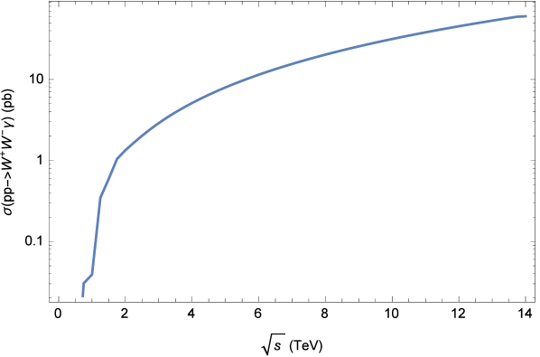
Figure 4: The total cross-section for the $W^{+}W^{-}\gamma$ production process as a function of the center-of-mass energy $\sqrt{s}$.

The central values of renormalization ($\mu_{R}$), and factorization ($\mu_{F}$) scales are set to $\mu_{R}=\mu_{F}=M_{W}$.

We calculated the transverse momentum ($p_{T}$) distributions in the region from 0.5 to 14 TeV of $W^{+}$ boson (for the $W^{-}$ boson transverse momentum distribution is analogous) in the final state for $pp\to W^{+}W^{-}\gamma$ process of the $\sqrt{s}=14\,\,TeV$. The results of our numerical calculations have been represented in Fig. 5.

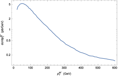
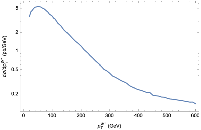
Figure 5: $W^{+}\,\,{\textrm{a}nd}\,\,W^{-}$ transverse momentum distributions at the center-of-mass energy $\sqrt{s}=14\,\,TeV$ in $pp$ interactions.

We now present the inclusive transverse-momentum spectrum of the $W$ vector-boson pair. We calculated the differential cross section for the transverse momentum ($p_{T}(WW)$) distribution of the $W$ boson pair in the regions $p_{T}=20\div 600\,\,GeV$ at the $\sqrt{s}=14\,\,TeV.$ We show our results of the transverse momentum distribution of the $W$- boson pair in Fig. 6.
It can be predicted that the feature of the $p_{T}$ distributions at the LHC characterize as searches in the triple gauge boson measurements.

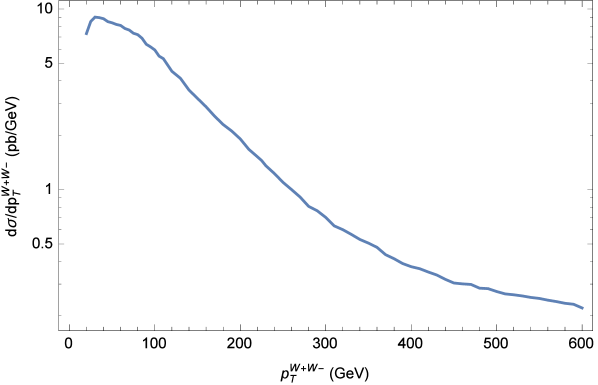
Figure 6: Transverse momentum distribution of the $W^{+}W^{-}$ pair at the center-of-mass energy $\sqrt{s}=14\,\,TeV$ in $pp$ interactions.

We will now study the distribution of the differential cross section on the rapidities ($y$) of $W^{+}$ and $W^{-}$ bosons in the final state. In Fig. 7, we present the rapidity ($y$) distributions, in the reqions $-2.5\leq y\leq 2.5$ of the final $W^{+}$ and $W^{-}$ bosons for the $pp\to W^{+}W^{-}\gamma$ process at $\sqrt{s}=14\,\,TeV$.

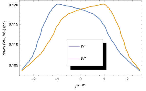
Figure 7: The rapidity distributions of the $W^{+}$ and $W^{-}$ bosons at the center-of-mass energy $\sqrt{s}=14\,\,TeV$ in $pp$ interactions: in the left peak ($W^{-}$), and in the right peak ($W^{+}$), respectively.

Also, we have calculated the distribution of the differential cross section for correlation of the rapidities between $W^{+}$ and $W^{-}$ bosons. The distribution of the correlation of rapidities is depicted in Fig. 8

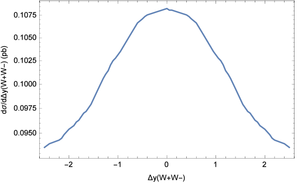
Figure 8: Distribution of the correlation of rapidity between $W^{+}$ and $W^{-}$ bosons: $\Delta y(W+W-)=y^{W+}-y^{W-}$, at the center-of-mass energy $\sqrt{s}=14\,\,TeV$.

IV Conclusion

In the present paper, we have studied the transverse momentum and rapidity distributions of vector bosons in proton - proton collisions.
We studied the $pp\rightarrow W^{+}W^{-}\gamma$ process using the quark (and anti-quark) distribution functions in the initial state set of the MSTW2008 MRSW parametrization in the framework of the Standard Model, which are intensively investigated in ATLAS and CMS at the Large Hadron Collider.
We have presented the numerical results for $W^{+}W^{-}\gamma$ production at LHC energy.
Having all the tools to calculate and using equation (49) together with the hard-scattering amplitude in equation (6) we performed the parton level calculations.

We estimated the cross section of the $W$ bosons production as a function of transverse momentum $p_{T}$ and rapidity $y$ of the $W$ bosons. The obtained results using the set of uPDFs MRSW can be used for such phenomenological studies. We used the experimental cuts of the transverse momentum and rapidity of the $W$ bosons used by the ATLAS and CMS experiments in their measurements, which are available to leading transverse momentum of lepton $p_{T}>20\,\,\,GeV$ and absolute value of rapidity $|\eta|<2.5$.
In this present paper, we investigated the distribution of the transverse momentum ($p_{T}$) and the rapidity ($y$) of $W^{+}$ and $W^{-}$ bosons separately, and also the distribution of the total cross section from the centre-of-mass energy $\sqrt{s}$ at LHC energy.
In this paper, we studied several cases of phenomenological interest, which demonstrate the effect of NLO corrections.
It can be predicted that the production of WW boson pair and $WW\gamma$ production is an important source of both the background for Higgs and the search for new physics at LHC.

References

- (1) V. M. Abazov et al., [D0 Collaboration], Phys. Rev. Lett. 108 (2012) 181803 [arXiv:1112.0536 [hep-ex]].
- (2) T. Aaltonen et al., [CDF Collaboration], CDF note 11098.
- (3) M. Aaboud et al., [ATLAS Collaboration], JHEP 1803 (2017) 042, [arXiv:1710.07235 [hep-ex]].
- (4) M. Aaboud et al., [ATLAS Collaboration], Eur.Phys.J. C 78 (2018) 24, [arXiv:1710.01123 [hep-ex]].
- (5) M. Aaboud et al., [ATLAS Collaboration], Eur.Phys.J. C 77 (2017) 563, [arXiv:1706.01708 [hep-ex]].
- (6) M. Aaboud et al.,[ATLAS Collaboration], Phys.Rev. D 95 (2017) 032001, [arXiv:1609.05122 [hep-ex]].
- (7) G. Aad et al. [ATLAS Collaboration], Eur. Phys. J. C 75 (2015) 209 [Erratum-ibid. C 75 (2015) 370] [arXiv:1503.04677 [hep-ex]].
- (8) G. Aad et al., [ATLAS Collaboration], Phys. Rev. D 87 (2013) 11, 112001 [Erratum-ibid. D 88 (2013) 7, 079906] [arXiv:1210.2979 [hep-ex]].
- (9) A.M. Sirunyan et al.,[CMS Collaboration], Phys. Rev. D 97 (2018) 072006 [arXiv:1708.05379 [hep-ex]].
- (10) A.M. Sirunyan et al., [CMS Collaboration], Phys. Lett. B 774 (2017) 533 [arXiv:1705.09171 [hep-ex]].
- (11) A.M. Sirunyan et al., [CMS Collaboration], Phys. Lett. B 772 (2017) 21 [arXiv:1703.06095 [hep-ex]].
- (12) A.M. Sirunyan et al., [CMS Collaboration], JHEP 1703 (2017) 162 [arXiv:1612.09159 [hep-ex]].
- (13) S. Chatrchyan et al., [CMS Collaboration], Eur. Phys. J. C 73 (2013) 2610 [arXiv:1306.1126 [hep-ex]].
- (14) S. Chatrchyan et al., [CMS Collaboration], Phys. Lett. B 721 (2013) 190 [arXiv:1301.4698 [hep-ex]].
- (15) ATLAS Collaboration, ATLAS-CONF-2014-033.
- (16) T. Gehrmann et al., Phys. Rev. Lett. 113 (2014) 212001, [arXiv:1408.5243 [hep-ph]]
- (17) M. Grazzini et al., JHEP 08 (2016) 140, [arXiv:1605.02716 [hep-ph]]
- (18) D. Curtin, P. Meade and P. J. Tien, arXiv:1406.0848 [hep-ph].
- (19) J. S. Kim, K. Rolbiecki, K. Sakurai and J. Tattersall, [arXiv:1406.0858 [hep-ph]].
- (20) H. Luo, M. x. Luo, K. Wang, T. Xu and G. Zhu, [arXiv:1407.4912 [hep-ph]].
- (21) J. Kalinowski et al., [arXiv: 1802.02366 [hep-ph]], CERN-TH-2017-269.
- (22) A. Fadol et al., J. Phys. Conf. Ser. 889 (2017) no.1, 012001.
- (23) E. Cheremushkina, Phys. Part. Nucl. 48 (2017) 752.
- (24) J. Campbell et al., PoS ICHEP 2016 (2016) 686, [arXiv: 1611.01700 [hep-ph]].
- (25) R. Boughezal, C. Focke, X. Liu and F. Petriello, W-boson production in association with a jet at next-to-next-to-leading order in perturbative QCD, Phys. Rev. Lett. 115 (2015) no.6,062002 [arXiv:1504.02131 [hep-ph]]; R. Boughezal, J. M. Campbell, R. K. Ellis, C. Focke, W. T. Giele, X. Liu and F. Petriello, Z-boson production in association with a jet at next- to-next-to-leading order in perturbative QCD, Phys. Rev. Lett.116 (2016) no.15, 152001 [arXiv:1512.01291 [hep-ph]]; A. Gehrmann-De Ridder, T. Gehrmann, E. W. N. Glover, A. Huss and T. A. Morgan, Z+jet production at NNLO, arXiv:1607.01749 [hep-ph].
- (26) J. M. Lindert et al., Eur. Phys. J. C 77, no. 12, 829 (2017) doi:10.1140/epjc/s10052-017-5389-1 [arXiv:1705.04664 [hep-ph]].
- (27) J. Collins, Foundations of perturbative QCD. Cambridge University Press, 2013.
- (28) M. G. Echevarria, A. Idilbi and I. Scimemi, Phys. Lett. B726(2013) 795 801, [1211.1947].
- (29) M. Aaboud et al., [ATLAS Collaboration], Eur.Phys.J. C 77 (2017) 646, [arXiv:1707.05597 [hep-ex]].
- (30) S. Chatrchyan et al., [CMS Collaboration], Phys.Rev.D90 (2014) 032008 [arXiv:1404.4619 [hep-ex]].
- (31) A. Sokolenki, K. Bondarenko, A. Boyarsky, L. Shchutska, arXiv: 1802.06385 [hep-ph].
- (32) E. Yatsenko, arXiv:1708.06534 [hep-ex].
- (33) J.I. Djuvsland, For ATLAS Collaboration, arXiv:1708.07667 [hep-ex].
- (34) Bing Li, For ATLAS Collaboration, PoS EPS-HEP2017 (2017) 448.
- (35) B. Mele, P. Nason, G. Ridolfi, Nucl. Phys. B357 (1991) 409.
- (36) S. Frixione, P. Nason, G. Ridolfi, Nucl. Phys. B383 (1992) 3.
- (37) S. Frixione, Nucl. Phys. B410 (1993) 280.
- (38) L. Dixon, Z. Kunszt, A. Signer, Nucl. Phys. B531 (1998) 3.
- (39) S. Dittmaier, S. Kallweit, P. Uwer, Nucl.Phys. B826 (2010) 18, arXiv: 0908.4124 [hep-ph].
- (40) J.M. Campbell, D.J. Miller, T. Robens, Phys.Rev.D92 (2015) 014033, arXiv: 1506.04801 [hep-ph].
- (41) W.J. Stirling, A. Werthenbach, Eur. Phys. J. C 12 (2000) 441.
- (42) S. Chatrchyan et al., [CMS Collaboration], Phys. Lett. B 721 (2013) 190, [arXiv:1301.4608 [hep-ex]].
- (43) S. Chatrchyan et al., [CMS Collaboration], Eur.Phys.J. C73 (2013) 2283, [arXiv:1210.7544 [hep-ex]].
- (44) K. Hagiwara, R.D.Peccei, D. Zeppenfeld and K. Hikasa, Nucl. Phys. B 282 (1987) 253.
- (45) J. Ellison and J. Wudka, Ann. Rev. Nucl. Part. Sci. 48 (1998) 33; hep-ph/ 9804322.
- (46) U. Baur and E.L. Berger, Phys. Rev. D 41 (1990) 1476.
- (47) DELPHI, OPAL, LEP Electroweak, ALEPH, L3 collaboration, S. Schael et al., Electroweak Measurements in Electron-Positron Collisions at W-Boson-Pair Energies at LEP ,Phys. Rept.532 (2013) 119 244, [1302.3415].
- (48) S.Atag and I.T.Cakir, Phys. Rev. D 63, 033004 (2001); arXiv: 0004089 [hep-ph].
- (49) S.Atag and I. Sahin, Phys. Rev. D 64, 095002 (2001).
- (50) I. Sahin and A.A. Billur Phys. Rev. D 83, 035011 (2011); arXiv: 1101.4998 [hep-ph].
- (51) I.T.Cakir, O.Cakir, A. Senol, A.T. Tasci, Acta Phys.Polon.B45, 10,1947 (2014); arXiv: 1406.7696 [hep-ph].
- (52) B. Sahin, Phys.Scripta 79, 065101 (2009).
- (53) J.Papavassiliou and K.Philippides, Phys.Rev.D 60, 113 007 (1999); arXiv: 9907376 [he-ph].
- (54) D. Choudhury, J. Kalinowski and A. Kulesza, Phys.Lett.B 457, 193 (1999); arXiv: 9904215 [hep-ph].
- (55) E. Chapon, C. Royon and O. Kepka, Phys.Rev.D 81, 074003 (2010); arXiv: 0912.5161 [hep-ph].
- (56) V. Arı, A. A. Billur, S.C. İnan, M. Köksal, Nuclear Physics B 906 (2016) 211 , arXiv: 1506.08998 [hep-ph]
- (57) B. Sahin, Mod.Phys.Lett. A32 (2017) 1750205.
- (58) A.D. Martin, W.J. Stirling, R.S. Thorne, G. Watt, Eur.Phys. J. C63 (2009) 189; arXiv: 0901.0002 [hep-ph].