Absorption Cross-Section and Decay Rate of Dilatonic Black Strings

Abstract

We studied in detail the propagation of a massive tachyonic scalar field in the background of a five-dimensional ($5D$) Einstein–Yang–Mills–Born–Infeld–dilaton black string: the massive Klein–Gordon equation was solved, exactly. Next we obtained complete analytical expressions for the greybody factor, absorption cross-section, and decay-rate for the tachyonic scalar field in the geometry under consideration. The behaviors of the obtained results are graphically represented for different values of the theory’s free parameters. We also discuss why tachyons should be used instead of ordinary particles for the analytical derivation of the greybody factor of the dilatonic $5D$ black string.

I Introduction

A wealth of information about quantum gravity can be obtained by studying the unique and fascinating objects known as black holes (BHs). In BH physics, greybody factors (GFs) modify black-body radiation, or predicted Hawking radiation SHR1 ; SHR2 , within the limits of geometrical optics Optics . In other words, GFs modify the Hawking radiation spectrum observed at spatial infinity (SI), so that the radiation is not pure Planckian Tez .

GF, absorption cross-section (ACS), and decay-rate (DR) are quantities dependent upon both the frequency of radiation and the geometry of spacetime. Currently, although there are many studies of GF, ACS, and DR (see for example GF1 ; GF2 ; GF3 ; GF4 ; GF5 ; GF6 and the references therein), the number of analytical studies of GFs that consider modified black-body radiation of higher dimensional ($D>4$) spacetimes, like the BHs in string theory and black strings BSs ; BSs2 ; BSs3 , is rather limited (see for instance GF2 ; GF3 ; BS1 ; BS2 ; BS3 ; BS4 ; BS5 ). This paucity of studies has arisen from the mathematical difficulty of obtaining an analytical solution to the wave equation of the stringent geometry being considered; in fact, analytical GF computations apply to spacetimes in which the metric components are independent of time. It is also worth noting that although BSs are defined as a higher dimensional generalization of a BH, in which the event horizon is topologically equivalent to $S^{2}\times S^{1}$ and spacetime is asymptotically $M^{D-1}\times S^{1}$ four-dimensional ($4D$) BSs are also derived.Lemos and Santos lem1 ; lem2 ; santos showed that cylindrically symmetric static solutions, with a negative cosmological constant, of the Einstein–Maxwell equations admit charged $4D$ BSs. A rotating version of the charged $4D$ BSs lem3 ; lem4 exhibits features similar to the Kerr-Newman BH in spherical topology. The problem of analyzing GFs of scalar fields from charged $4D$ BSs has recently been discussed by Ahmed and Saifullah ahmed . An interesting point about GFs has been reported by dof : BH energy loss during Hawking radiation depends, crucially, on the GF and the particles’ degrees of freedom.

As mentioned above, further study of the GFs of BSs is required. To fill this literature gap, in the current study, we considered dilatonic $5D$ BS Habib , which is a solution to Einstein–Yang–Mills–Born–Infeld–dilaton (EYMBID) theory. We analytically studied its GF, ACS, and DR for massive scalar fields; however, we considered tachyonic scalar particles instead of ordinary ones. The main reason for this consideration is that using ordinary mass in the Klein–Gordon equation (KGE) of the dilatonic $5D$ BS (as will be explained in detail later) leads to the diverging of GFs. Roughly speaking, this is due to the flux of the propagating waves of the ordinary massive scalar fields. Namely, once the scalar fields to be considered belong to the massive ordinary particles, the incoming SI flux becomes zero. The latter remark implies that detectable radiation emitted from a dilatonic $5D$ BS spacetime belongs to the massive tachyonic scalar fields. Therefore, the current study focuses on the wave dynamics of tachyonic particles moving in dilatonic $5D$ BS spacetime. However, using tachyonic modes in $5D$ geometry should not be seen as nonphysical; instead they should be considered as the imaginary mass fields rather than to faster-than-light particles mytachyon . First, Feinberg Feinberg ; Feinberg2 proposed that tachyonic particles could be quanta of a quantum field with imaginary mass. It was soon realized that excitations of such imaginary mass fields do not in fact propagate faster than light immass .

Following the idea of Kaluza–Klein KK , any $4D$ physical trajectory is the projection of higher dimensional worldlines. Effective $4D$ worldlines associated with massive particles are causality constrained to be timelike. However, the corresponding higher dimensional worldlines need not be exclusively timelike, which gives rise to a topological classification of physical objects. In particular, elementary particles in a $5D$ geometry should be viewed as tachyonic modes. The existence of tachyons in higher dimensions has been thoroughly studied by Davidson and Owen PLB . Furthermore, the reader may refer to Horowitz to understand tachyon condensation in the evaporation process of a BS. To find the analytical GF, ACS, and DR, we have shown how to obtain the complete analytical solution to the massive KGE in the geometry of a dilatonic $5D$ BS.

Our work is organized as follows. Following this introduction, a brief overview of the geometry of the dilatonic $5D$ BS is provided in Sec. 2. Section 3 describes the KGE of the tachyonic fields in the dilatonic $5D$ BS geometry; we present the exact solution of the radial equation in terms of hypergeometric functions. In Sec. 4, we compute the GF and consequently the ACS and DR of the dilatonic $5D$ BS, respectively. We then graphically exhibit the results of the ACS and DR. Section 5 concludes with the final remarks drawn from our study.

II Dilatonic $5D$ BS in EYMBID Theory

$D\left(=d+1\right)$-dimensional action in the EYMBID theory is given by Habib

$$I_{EYMBID}=-\frac{1}{16\pi G_{(D)}}\int_{\mathcal{M}}d^{d}x\sqrt{-g}\Bigg{[}\mathcal{R}-\frac{4\left(\bigtriangledown\psi\right)^{2}}{D-2}+$$

$$4\chi^{2}e^{-b\psi}\left(1-\sqrt{1+\frac{Fe^{2b}}{2\chi^{2}}}\right)\Bigg{]},$$ (1)

where $\psi$ is the dilaton field, $\chi$ denotes the Born-Infeld parameter Born , and $b=-\frac{4}{d-2}\alpha$ with the dilaton parameter $\alpha=\frac{1}{\sqrt{d-1}}$. $G_{(D)}$ represents the $D$-dimensional Newtonian constant and its relation to its $4D$ form $\left(G_{(4)}\right)$ is given by

$$G_{(D)}=G_{(4)}L^{D-4},$$ (2)

where $L$ is the upper limit of the compact coordinate $\left(\int_{0}^{L}dz=L\right)$. Furthermore, $\mathcal{R}$ stands for the Ricci scalar and $F=F_{\lambda\rho}^{(\overline{a})}F^{(\overline{a})\lambda\rho}$ where the 2-form Yang-Mills field is given by

$$F^{(a)}=dA^{(\overline{a})}+\frac{1}{2\sigma}C_{(\overline{b})(\overline{c})}^{(\overline{a})}\left(A^{(\overline{b})}\wedge A^{(\overline{c})}\right),$$ (3)

with $C_{(\overline{b})(\overline{c})}^{(\overline{a})}$ and $\sigma$ being structure and coupling constants, respectively. The Yang-Mills potential $A^{(a)}$is defined by following the Wu-Yang ansatz Wu

$$A^{(\overline{a})}=\frac{Q}{r^{2}}\left(x_{i}dx_{j}-x_{j}dx_{i}\right),$$ (4)

$$r^{2}=\underset{i=1}{\overset{d-1}{\sum}}x_{i}^{2},\text{ }2\leq j+1\leq i\leq d-1,1\leq\overline{a}\leq(d-1)(d-2)/2,$$ (5)

where $Q$ is the Yang-Mills charge. The solution for the dilaton is as follows

$$\psi=-\frac{\left(d-2\right)}{2}\frac{\alpha\ln r}{\alpha^{2}+1}.$$ (6)

On the other hand, the line-element of the dilatonic $5D$ BS is given by Habib

$$ds_{0}^{2}=-\frac{f(r)}{\beta}d\widetilde{t}^{2}+\frac{\beta dr^{2}}{rf(r)}+rd\widetilde{z}^{2}+\beta\left(d\theta^{2}+\sin^{2}\theta d\phi^{2}\right),$$ (7)

where $f(r)=r-r_{+}$ and $\beta=\frac{4Q^{2}}{3}$. $r_{+}$ represents the outer event horizon having the following $(d+1)-$dimensional form:

$$\frac{32}{L^{d-4}}\left(\frac{Q^{2}d}{d-1}\right)^{\frac{d-2}{2}}=r_{+}^{\frac{d(d-2)+2}{d}}.$$ (8)

Because, in our case, $D=5$ $\left(\text{i.e., }d=4\right)$, the horizon becomes

$$r_{+}=4\beta^{\frac{2}{5}}=4.488Q^{\frac{4}{5}}.$$ (9)

After rescaling the metric (7)

$$ds^{2}=\frac{ds_{0}^{2}}{\beta}=-\frac{f(r)}{\beta^{2}}d\widetilde{t}^{2}+\frac{dr^{2}}{rf(r)}+\frac{r}{\beta}d\widetilde{z}^{2}+d\theta^{2}+\sin^{2}\theta d\phi^{2},$$ (10)

and in sequel assigning $\widetilde{t}$ and $\widetilde{z}$ coordinates to the new coordinates:

$$\widetilde{t}\rightarrow\beta t,\text{ \ \ \ \ \ }\widetilde{z}\rightarrow\beta z,$$ (11)

we get the metric that will be used in our computations:

$$ds^{2}=-f(r)dt^{2}+\frac{dr^{2}}{rf(r)}+\beta rdz^{2}+d\theta^{2}+\sin^{2}\theta d\phi^{2}.$$ (12)

It is worth noting that the surface gravity SurGrav of the dilatonic $5D$ BS can be evaluated by

$$\kappa^{2}=-\frac{1}{2}\left.\triangledown^{\rho}\Upsilon^{\sigma}\triangledown_{\rho}\Upsilon_{\sigma}\right|_{r=r_{+}},$$ (13)

in which $\Upsilon^{\mu}$ represents the timelike Killing vector:

$$\Upsilon^{\mu}=[1,0,0,0,0].$$ (14)

Then, Eq.(13) results in

$$\kappa=\left.\frac{\sqrt{r}f^{\prime}}{2}\right|_{r=r_{+}}=\frac{\sqrt{r_{+}}}{2},$$ (15)

where the prime denotes the derivative with respect to $r$. Furthermore, the associated Hawking temperature is expressed by

$$T_{H}=\frac{\kappa}{2\pi}=\frac{\sqrt{r_{+}}}{4\pi}.$$ (16)

It is important to remark that the Hawking temperature of the dilatonic BS given in Eq. (40) of Ref. Habib is incorrect. The authors of Ref. Habib computed the Hawking temperature of the dilatonic $5D$ BS considering the metric to be symmetric, which is not the case since $g_{tt}\neq\frac{1}{g_{rr}}$. Meanwhile, it is obvious that dilatonic $5D$ BS (12) has a non-asymptotically flat structure. Therefore, it possesses a quasilocal mass BY1 ; BY2 ; BY3 , which can be computed as follows

$$M_{QL}=\frac{1}{6}\beta r_{h}^{\frac{3}{2}}L=\frac{4}{3}\beta^{\frac{8}{5}}L\cong 2.113Q^{\frac{16}{5}}L.$$ (17)

Thus, the first law of thermodynamics is satisfied:

$$dM_{QL}=T_{H}dS_{BH},$$ (18)

where $S_{BH}$ denotes the Bekenstein-Hawking entropy SurGrav , which takes the following form for the dilatonic $5D$ BS

$$S_{BH}=\frac{A_{H}}{4}=\frac{1}{4}\beta r_{h}\int_{0}^{\pi}\sin\theta d\theta\int_{0}^{2\pi}d\phi\int_{0}^{L}dz=\pi\beta Lr_{h}.$$ (19)

III Wave Equation of a Massive Scalar Tachyonic Field in Dilatonic $5D$ BS

As the scalar waves being studied belong to the massive scalar tachyons, the corresponding KGE is given by

$$\left[\square-\left(i\mu\right)^{2}\right]\Psi(t,\mathbf{r})=\left[\square+\mu^{2}\right]\Psi(t,\mathbf{r})=0.$$ (20)

We chose ansatz as follows:

$$\Psi(t,\mathbf{r})=R(r)Y_{l}^{m}(\theta,\phi)e^{ikz}e^{-i\omega t},$$ (21)

where $Y_{l}^{m}(\theta,\phi)$ is the usual spherical harmonics and $k$ is a constant. After making straightforward calculations, we obtained the radial equation as follows:

$$rf\frac{\overset{\cdot\cdot}{R}}{R}+\frac{\overset{\cdot}{R}}{R}\left(f+r\overset{\cdot}{f}\right)+\frac{\omega^{2}}{f}-\frac{k^{2}}{\beta r}+\mu^{2}-\lambda=0,$$ (22)

where $\lambda=l(l+1)$ and a dot mark denotes a derivative with respect to $r$. Multiplying each term by $r\beta f(r)R(r)$ and using the ansatz $y=\frac{r_{+}-r}{r_{+}}$, which in turn implies $r=r_{+}-yr_{+}$, one gets

$$y(1-y)R^{\prime\prime}+(1-2y)R^{\prime}+\left[\frac{\omega^{2}}{yr_{+}}+\frac{k^{2}}{\beta(1-y)r_{+}}-\mu^{2}+\lambda\right]R=0,$$ (23)

where prime denotes derivative with respect to $y$. Setting

$$\left[\frac{\omega^{2}}{yr_{+}}+\frac{k^{2}}{\beta(1-y)r_{+}}-\mu^{2}+\lambda\right]=\frac{A^{2}}{y}-\frac{B^{2}}{1-y}+C,$$ (24)

one can obtain

$$A = -\frac{\omega}{2\kappa},$$

$$B = \frac{ik}{2\kappa\sqrt{\beta}},$$ (25)

$$C = \lambda-\mu^{2}.$$

Equation (23) can be solved by comparing it with the standard hypergeometric differential equation Steg which admits the following solution:

$$R = \xi_{1}\left(-y\right)^{iA}\left(1-y\right)^{-B}F\left(a,b;c;y\right)+$$ (26)

$$\xi_{2}\left(-y\right)^{-iA}\left(1-y\right)^{-B}F\left(\alpha,\varsigma;\eta;y\right),$$

where

$$a=\frac{1}{2}\left(1+\sqrt{1+4C}\right)+iA-B,$$ (27)

$$b=\frac{1}{2}\left(1-\sqrt{1+4C}\right)+iA-B,$$ (28)

$$c=1+2iA.$$ (29)

and

$$\alpha=a-c+1,$$ (30)

$$\varsigma=b-c+1,$$ (31)

$$\eta=2-c.$$ (32)

According to our calculations, to have a non-zero SI incoming flux [see Eq. (53)] or non-divergent GF [see Eq.(55)] , $\sqrt{1+4C}$ must be imaginary. To this end, we must impose the following condition:

$$4\mu^{2}>4\lambda+1,$$ (33)

such that

$$\sqrt{1+4C}=i\tau,$$ (34)

where

$$\tau=\sqrt{4\mu^{2}-4\lambda-1},\tau\in\mathbb{R}.$$ (35)

To obtain a physically acceptable solution, we must terminate the outgoing solution at the horizon, which can be simply done by imposing $\xi_{1}=0$. Thus, the physical radial solution reduces to

$$R=\xi_{2}\left(-y\right)^{-iA}\left(1-y\right)^{-B}F\left(\alpha,\varsigma;\gamma;y\right).$$ (36)

It should be noted that checking the forms of Eq. (36) both at the horizon and at SI is essential. Section 3 shows that both are needed for the evaluation of the GF. For the near horizon (NH) where $y\rightarrow 0$, one can state:

$$R_{NH}=\xi_{2}\left(-y\right)^{-iA},$$ (37)

which implies that the purely ingoing plane wave reads

$$\psi_{NH}=\xi_{2}e^{-i\omega(\widehat{r}_{\ast}+t)}e^{ikz},$$ (38)

where

$$r^{{}_{\ast}} = \int\frac{dr}{\sqrt{r}f}\text{ \ }\rightarrow\text{ \ \ }\widehat{r}_{\ast}=\lim_{r\rightarrow r_{+}}r^{{}_{\ast}}\simeq\frac{\ln\left(-y\right)}{\sqrt{r_{+}}},$$

$$\widehat{r}_{\ast} \simeq \frac{1}{2\kappa}\ln\left(-y\right)\text{ \ }\Longrightarrow\text{\ \ }y=-e^{2\kappa\widehat{r}_{\ast}}.$$ (39)

On the other hand, for $y\rightarrow\infty$, the inverse transformation of the hypergeometric function is given by Lay

$$F\left(\alpha,\varsigma;\eta;y\right) =\left(-y\right)^{-\alpha}\frac{\Gamma(\eta)\Gamma(\varsigma-\alpha)}{\Gamma(\varsigma)\Gamma(\eta-\alpha)}\times$$

$$F\left(\alpha,\alpha+1-\eta;\alpha+1-\varsigma;1/y\right)+$$

$$\left(-y\right)^{-\varsigma}\frac{\Gamma(\eta)\Gamma(\alpha-\varsigma)}{\Gamma(\alpha)\Gamma(\eta-\varsigma)}\times$$

$$F\left(\varsigma,\varsigma+1-\eta;\varsigma+1-\alpha;1/y\right),$$ (40)

which yields the following asymptotic solution

$$R_{SI} \backsimeq \xi_{2}\left(-y\right)^{-iA-B-\alpha}\frac{\Gamma(\eta)\Gamma(\varsigma-\alpha)}{\Gamma(\varsigma)\Gamma(\eta-\alpha)}+$$ (41)

$$\xi_{2}\left(-y\right)^{-iA-B-\varsigma}\frac{\Gamma(\eta)\Gamma(\alpha-\varsigma)}{\Gamma(\alpha)\Gamma(\eta-\varsigma)}.$$

To express Eq.(41) in a more compact form, let us perform the following simplifications. Considering

$$-iA-B-\alpha=-\frac{1}{2}\left(1+i\tau\right),$$ (42)

together with

$$-iA-B-\varsigma=-\frac{1}{2}\left(1-i\tau\right),$$ (43)

and letting $x=-y$, the radial equation for $r\rightarrow\infty$ takes the form

$$R_{SI}=\frac{1}{\sqrt{x}}\left[\xi_{2}x^{-\frac{i\tau}{2}}\frac{\Gamma(\eta)\Gamma(\varsigma-\alpha)}{\Gamma(\varsigma)\Gamma(\eta-\alpha)}+\xi_{2}x^{\frac{i\tau}{2}}\frac{\Gamma(\eta)\Gamma(\alpha-\varsigma)}{\Gamma(\alpha)\Gamma(\eta-\varsigma)}\right].$$ (44)

One can express $x$ in terms of the tortoise coordinate at SI as

$$r^{{}_{\ast}}=\int\frac{dr}{\sqrt{r}f}\text{ \ }\rightarrow\text{ \ \ }\widehat{r}_{\ast}=\lim_{r\rightarrow\infty}r^{{}_{\ast}}\simeq-\frac{2}{\sqrt{r}},$$ (45)

such that

$$x=r-r_{+}\text{ \ \ \ }\left.x\right|_{r\rightarrow\infty}\simeq r=4e^{-2\widehat{r}_{\ast}},$$ (46)

where $\widehat{r}_{\ast}=\ln r^{{}_{\ast}}$. Therefore, we have

$$R_{SI}=\frac{1}{\sqrt{r}}\left[\Lambda_{1}e^{i\widehat{r}_{\ast}\tau}+\Lambda_{2}e^{-i\widehat{r}_{\ast}\tau}\right],$$ (47)

where

$$\Lambda_{1}=2^{-i\tau}\xi_{2}\frac{\Gamma(\eta)\Gamma(\varsigma-\alpha)}{\Gamma(\varsigma)\Gamma(\eta-\alpha)},$$ (48)

$$\Lambda_{2}=2^{-i\tau}\xi_{2}\frac{\Gamma(\eta)\Gamma(\alpha-\varsigma)}{\Gamma(\alpha)\Gamma(\eta-\varsigma)}.$$ (49)

Thus, the asymptotic wave solution becomes

$$\psi_{SI}=\frac{e^{ikz}}{\sqrt{r}}\left[\Lambda_{1}e^{i(\widehat{r}_{\ast}\tau-\omega t)}+\Lambda_{2}e^{-i(\widehat{r}_{\ast}\tau+\omega t)}\right].$$ (50)

IV Radiation of Dilatonic $5D$ BS

IV.1 The Flux Computation

In this section, we compute the ingoing flux at the horizon $\left(r\rightarrow r_{+}\right)$ and the asymptotic flux for the SI region $\left(r\rightarrow\infty\right)$. The evaluation of these flux values will enable us to calculate the GF and subsequently, the ACS and DR.

The NH-flux can be calculated via Fernando ; Flux

$$\digamma_{NH}=\frac{A_{BH}}{2i}\left(\overline{\psi}_{NH}\partial r_{\ast}\psi_{NH}-\psi_{NH}\partial r_{\ast}\overline{\psi}_{NH}\right),$$ (51)

which, after a few manipulations, can be written as

$$\digamma_{NH}=-4\pi\beta\left|\xi_{2}\right|^{2}r_{+}.$$ (52)

The incoming flux at SI is computed via

$$\digamma_{SI}=\frac{A_{BH}}{2i}\left(\overline{\psi}_{SI}\partial r_{\ast}\psi_{SI}-\psi_{SI}\partial r_{\ast}\overline{\psi}_{SI}\right).$$ (53)

Having performed the steps to evaluate the derivatives with respect to the tortoise coordinate, the incoming flux at SI takes the form

$$\digamma_{SI}=-4\pi\beta\left|\Lambda_{2}\right|^{2}\tau.$$ (54)

It is important to remark that if we were dealing with the standard particles rather than tachyons, $\tau$ (35) would be imaginary i.e., $\tau\rightarrow i\tau$ and therefore SI incoming wave would lead this flux evaluation (53) to be zero. This would indicate the existence of a divergent GF.

IV.2 ACS of Dilatonic $5D$ BS

The GF of the dilatonic $5D$ BS is obtained by the following expression GF2 ; GF4

$$\gamma^{l,k}=\frac{\digamma_{NH}}{\digamma_{SI}}=\frac{-4\pi\beta\left|\xi_{2}\right|^{2}r_{+}}{-4\pi\beta\left|\Lambda_{2}\right|^{2}\tau},$$ (55)

which is nothing but

$$\gamma^{l,k}=\frac{\left|\xi_{2}\right|^{2}r_{+}}{\left|\Lambda_{2}\right|^{2}\tau}.$$ (56)

After a few manipulations, with the following (see Steg )

$$\left|\Gamma(iy)\right|^{2}=\frac{\pi}{y\sinh\left(\pi y\right)},$$ (57)

$$\left|\Gamma(1+iy)\right|^{2}=\frac{\pi y}{\sinh\left(\pi y\right)},$$ (58)

$$\left|\Gamma(\frac{1}{2}+iy)\right|^{2}=\frac{\pi}{\cosh\left(\pi y\right)},$$ (59)

Eq. (56) can be presented as

$$\gamma^{l,k}=\frac{\kappa r_{+}}{\omega}\left(e^{\frac{2\pi\omega}{\kappa}}-1\right)\Xi,$$ (60)

where

$$\Xi=\frac{e^{2\pi\tau}-1}{\left[e^{\pi\left(\tau+\frac{\omega}{\kappa}-\frac{k}{\kappa\sqrt{\beta}}\right)}+1\right]\left[e^{\pi\left(\tau+\frac{\omega}{\kappa}+\frac{k}{\kappa\sqrt{\beta}}\right)}+1\right]}.$$ (61)

To evaluate the ACS of the dilatonic $5D$ BS concerned, we follow the study of Kanti . Thus, one can get the ACS expression in $5D$ as follows:

$$\sigma^{l,k}=\frac{4\pi\left(l+1\right)^{2}}{\omega^{3}}\gamma^{l,k},$$ (62)

which, in our case, becomes 

$$\sigma^{l,k}=\frac{4\pi\left(l+1\right)^{2}\kappa r_{+}}{\omega^{4}}\left(e^{\frac{2\pi\omega}{\kappa}}-1\right)\Xi.$$ (63)

Furthermore, one can also get the total ACS as follows tcs

$$\sigma_{abs}^{Total}=\sum\limits_{l=0}^{\infty}\sigma^{l,k}.$$ (64)

In Fig. 1., the relationship between absorption ACS and frequency is examined; the figure is drawn based on Eq. (63). In the high frequency regime, all ACSs tend to vanish by following the same curve. Unlike the high frequency regime, ACSs diverge in the low frequency regime as $\omega\rightarrow 0$. As a final remark, negative $\sigma^{l,k}$ behavior has not been observed in our graphical analyzes, which means that superradiance does not occur chandra , as expected (as the dilatonic $5D$ BS (12) does not rotate).

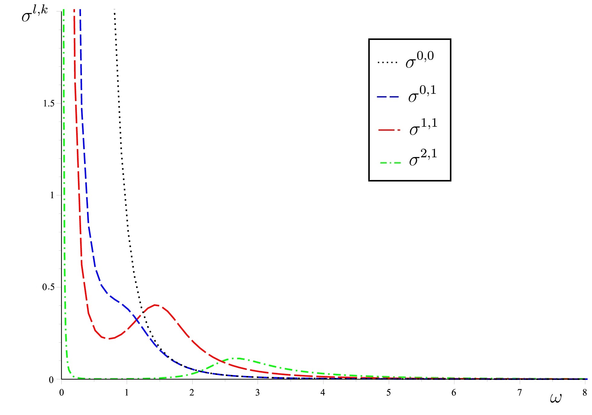
Figure 1: Plots of the ACS ($\sigma^{l,k}$) versus frequency $\omega$. The plots are governed by Eq. (63). The configuration of the dilatonic $5D$ BS is as follows $\mu=3$ and $Q=0.2$.

IV.3 DR of Dilatonic $5D$ BS

The final step follows from the ACS evaluation. The DR of the dilatonic $5D$ BS can be computed via GF4

$$\Gamma_{DR}^{l,k}=\frac{\sigma^{l,k}}{e^{\frac{2\pi\omega}{\kappa}}-1}=\frac{4\pi\left(l+1\right)^{2}\kappa r_{+}}{\omega^{4}}\Xi.$$ (65)

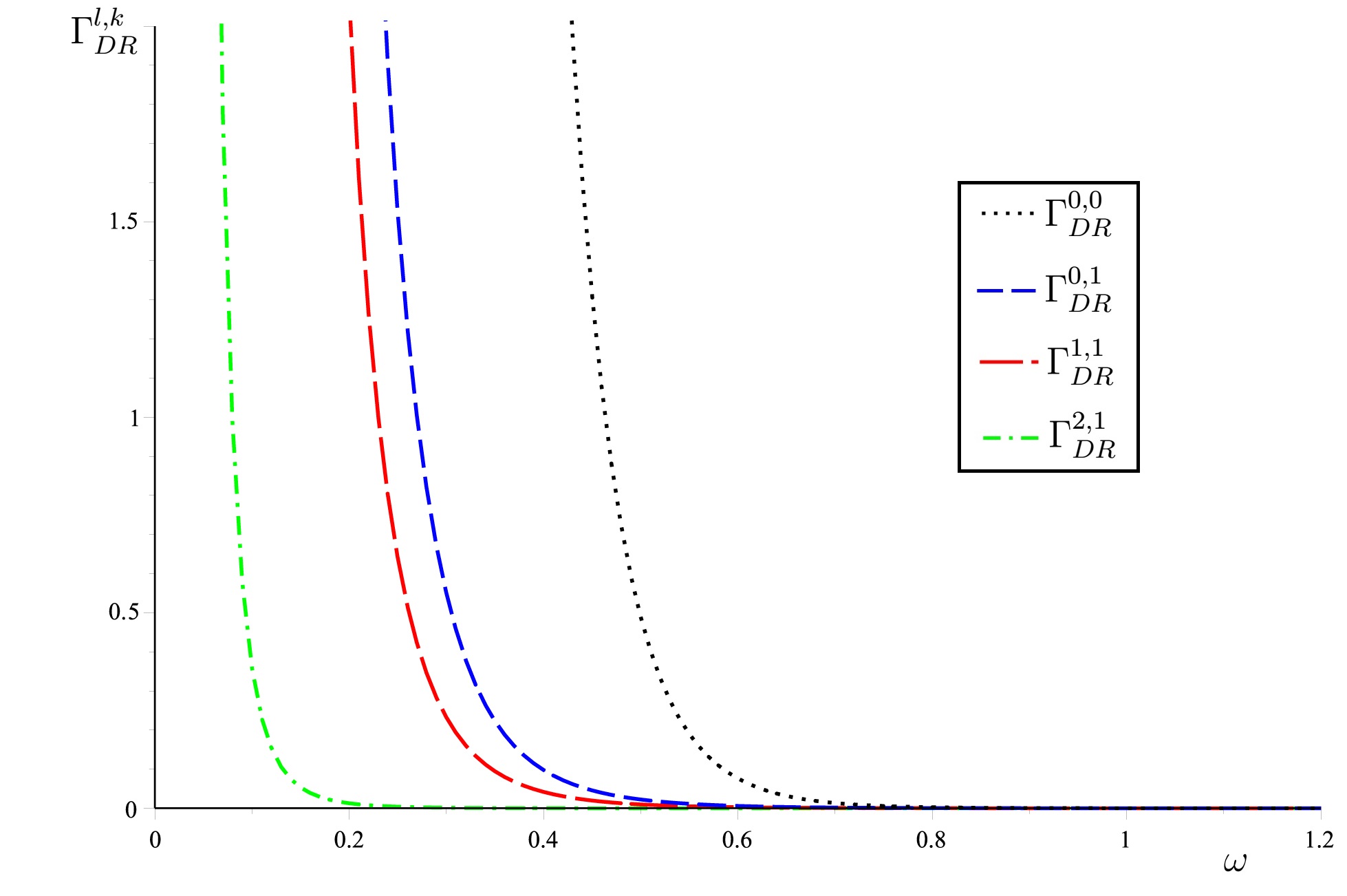
Figure 2: Plots of the DR $(\Gamma_{DR}^{l,k})$ versus frequency $\omega$. The plots are governed by Eq. (65). The configuration of the dilatonic $5D$ BS is as follows $\mu=3$ and $Q=0.2$.

Fig. 2. shows how the DR behaves with respect to the frequency. By taking Eq. (65) as the reference, the plots for increasing $l$ are illustrated. In the high frequency regime, all DRs fade in the same way. In the low frequency regime, DRs tend to diverge. However, it can be observed that when $l$ has larger values, the corresponding DR diverges when $\omega$ is much closer to zero.

V Conclusion

This article evaluated the GF, ACS, and DR for the dilatonic $5D$ BS geometry arising from the EYMBID theory. As a result of the analytical method we followed, it was shown that the radiation of the dilatonic $5D$ BS spacetime can only be caused by tachyons. The crucial point here is that if standard scalar particles had been used rather than tachyonic ones, zero incoming flux at SI would have been obtained, which would lead to the diverging of the GF. Therefore, in a way, we were forced to use tachyons to solve this problem, and this carries great importance as it implies that the fifth dimension could be directly linked to tachyons. In short, according to our analytical method, we obtained results (compatible with boundary conditions) when the radiation of the dilatonic $5D$ BS was provided by the tachyons.

In future study, we want to extend our analysis to the Dirac equation for the geometry of the dilatonic $5D$ BS. Hence, we are planning to undertake similar analysis for fermions and compare the results with scalar ones .

References

- (1) S. W. Hawking, Nature, 248, 30 (1974).
- (2) S. W. Hawking, Commun. Math. Phys., 43, 199 (1975); erratum: ibid, 46, 206 (1976).
- (3) S. Creek, O. Efthimiou, P. Kanti, and K. Tamvakis, Phys. Rev. D 75, 084043 (2007).
- (4) P. Boonserm, Rigorous bounds on Transmission, Reflection, and Bogoliubov coefficients, arXiv:0907.0045 (2009).
- (5) C. Ding, S. Chen, and J. Jing, Phys. Rev. D 82, 024031 (2010).
- (6) T. Harmark, J. Natario, and R. Schiappa, Adv. Theor. Math. Phys. 14, 727 (2010).
- (7) P. Kanti, T. Pappas, and N. Pappas, Phys. Rev. D 90, 124077 (2014).
- (8) I. Sakalli and O. A. Aslan, Astropar. Phys. 74, 73 (2016).
- (9) G. Panotopoulos and A. Rincon, Phys. Rev. D 96, 025009 (2017).
- (10) C-Y. Zhang, P-C. Li, and B. Chen, Phys. Rev. D 97, 044013 (2018).
- (11) J. Kunz, Black Holes In Higher Dimensions (Black Strings And Black Rings), The Thirteenth Marcel Grossmann Meeting: pp. 568-581 (2015); doi.org/10.1142/9789814623995_0027.
- (12) R. Gregory and R. Laflamme, Nucl. Phys. B 428, 399 (1994).
- (13) R. Gregory and R. Laflamme, Phys. Rev. Lett. 70, 2837 (1993).
- (14) I. R. Klebanov and S. D. Mathur, Phys. Nucl. Phys. B 500, 115 (1997).
- (15) C. G. Callan, S. S. Gubser, I. R. Klebanov, and A. A. Tseytlin, Nucl. Phys. B 489, 65 (1997).
- (16) M. Cvetic and F. Larsen, Phys. Rev. D 56, 4994 (1997).
- (17) I. R. Klebanov and M. Krasnitz, Phys. Rev. D 55, R3250 (1997).
- (18) S. S. Gubser and I. R. Klebanov, Nucl. Phys. B 482, 173 (1996).
- (19) J. P. S. Lemos, Class. Quant. Grav. 12, 1081 (1995).
- (20) J. P. S. Lemos, Phys. Lett. B 352, 46 (1995).
- (21) N. O. Santos, Class. Quant. Grav. 10, 2401 (1993).
- (22) J. P. S. Lemos and V. T. Zanchin, Phys. Rev. D 54, 3840 (1996).
- (23) R. G. Cai and Y. Z. Zhang, Phys. Rev. D 54, 4891 (1996).
- (24) J. Ahmed and K. Saifullah, Eur. J. C 77, 885 (2017).
- (25) M. Cavaglia, Phys. Lett. B 569, 7 (2003).
- (26) S. H. Mazharimousavia and M. Halilsoy, Eur. Phys. J. Plus 131, 138 (2016).
- (27) A. Sen, JHEP 0204, 048 (2002).
- (28) G. Feinberg, Phys. Rev. 159, 1089 (1967).
- (29) G. Feinberg, Phys. Rev. D 17, 1651 (1978).
- (30) Y. Aharonov, A. Komar, and L. Susskind, Phys. Rev. 182, 1400 (1969).
- (31) Th. Kaluza, Sitz. Preuss. Akad. Wiss. Berlin (Math. Phys.) 966 (1921); O. Klein, Z. Phys. 37, 895 (1926).
- (32) A. Davidson and D. A. Owen, Phys. Lett. B 177, 77 (1986).
- (33) G. Horowitz, JHEP 0508, 091 (2005).
- (34) M. Born and L. Infeld, Proc. Roy. Soc. Lond. A 144, 425 (1934).
- (35) T.T. Wu, C.N. Yang, in Properties of Matter Under Unusual Conditions, edited by H. Mark and S. Fernbach, (Interscience, New York, 1969).
- (36) S. Fernando, Gen. Rel. Grav. 37, 461 (2005).
- (37) C. Ding, S. Chen, and J. Jing, Phys. Rev. D 82, 024031 (2010).
- (38) R. M. Wald, General Relativity (The University of Chicago Press, Chicago and London, 1984).
- (39) J. D. Brown and J. W. York, Phys. Rev. D 47, 1407 (1993).
- (40) S. Bose and N. Dadhich, Phys.Rev. D 60, 064010 (1999).
- (41) S. Chakraborty and N. Dadhich, JHEP 12, 003 (2015).
- (42) M. Abramowitz and I. A. Stegun, Handbook of Mathematical Functions (Dover, New York, 1965).
- (43) S. Y. Slavyanov and W. Lay, Special Functions: A Unified Theory Based on Singularities (Oxford Mathematical Monographs, New York, 2000).
- (44) P. Kanti, J. Grain and A. Barrau, Phys. Rev. D 71,104002 (2005).
- (45) W. G. Unruh, Phys. Rev. D 14, 3251 (1976).
- (46) S. Chandrasekhar, The Mathematical Theory of Black Holes (Oxford University Press, New York, 1983).