Hill’s nano-thermodynamics is equivalent with Gibbs’ thermodynamics for curved surfaces

Abstract

We review first how properties of curved surfaces can be studied using Hill’s thermodynamics, also called nano-thermodynamics. We proceed to show for the first time that Hill’s analysis is equivalent to Gibbs for curved surfaces. This simplifies the study of surfaces that are curved on the nano-scale, and opens up a possibility to study non-equilibrium systems in a systematic manner.

1 Introduction

To master transport on the nano-scale, say in catalysis, for electrode reactions or for fluid transport in porous media, is of great importance [1,2,3]. But systems on this scale do not have additive thermodynamic properties [4,5,6], and this makes their thermodynamic description complicated. Hill [4,5] devised a scheme to obtain thermodynamics properties at equilibrium for this scale in the early 1960’ies. He showed that the thermodynamics on this scale was crucially modified, a fact that may have hampered the further development since then. Nevertheless, he provided a systematic basis, which is also the first necessary step in a development of a non-equilibrium thermodynamics theory. We believe that Hill’s method is better suited, to make progress in the direction of non-equilibrium. To facilitate its use, it may then be useful to make it better anchored in the more familiar thermodynamic description of Gibbs. This communication addresses how this can be done for curved surfaces, a central topic in nano-scale physics.

Gibbs [7] gave a thermodynamic theory of equilibrium surfaces; a theory that was extended by Tolman [8] and Helfrich [9]. Tolman [8] introduced what is now called the Tolman-length, while Helfrich [9] gave an expansion to second order in the curvature and introduced two bending rigidities and the natural curvature. Blokhuis and Bedeaux [10-12] derived statistical mechanical expressions for these coefficients.

Hill chose a different route to this problem with his small system thermodynamics. He introduced an ensemble of small systems, and used the replica energy to obtain thermodynamic properties that depended on the surface area and curvatures.

Both Hill and Gibbs described how to account for thermodynamic contributions from curved surfaces. This implies that Hill’s analysis should reproduce the description given by Gibbs. Hill [4, page 168] only addressed this issue for the special case of a spherical drop in a super saturated vapor. We have recently verified that this is generally true for a flat surface [13]. In this letter we verify this property for curved surfaces. Doing this, we verify that the properties of curved surfaces on the nanoscale can be studied also by Hill’s method.

This has at least two consequences. First, we can better understand why a relatively new method, the small system method [13,14], can be used to produce properties of the surface, even if there is no direct study of surfaces in the method. We are able to conclude that all information, even of the surface of a system, can be obtained from the fluctuations of the number of particles and the energy in the small system. Second, it supports Hill’s idea to deal with nano-scale systems as ensembles. This we expect will facilitate a derivation of non-equilibrium properties like the entropy production and flux-force relations [15].

Before we study the equivalence of Hill’s method with Gibbs’, we give a short repetition of the essential points of Hill’s method. We then discuss the curvature dependencies in detail. Doing this, we hope to revitalize Hill’s work [4,5] and contribute to the contemporary need for a more systematic nano-scale thermodynamics away from equilibrium.

2 The idea of Hill’s method

We recapitulate the essentials of Hill’s method. Consider a small system with volume $V$ in contact with the environment of temperature $T$ and chemical potential $\mu$. The system can exchange heat and particles with the environment. An ensemble of replicas is now constructed by considering $\mathcal{N}$ independent, distinguishable small systems, characterized by $T$, $V$, $\mu$. Figure 1 shows two replicas in contact with the heat- and particle-bath of the environment. The environment defines $T$ and $\mu$.

The idea is now that the ensemble of small systems follows the laws of macroscopic thermodynamic systems when $\mathcal{N}$ is large enough. The Gibbs equation for the ensemble is given by

$$dU_{t}=TdS_{t}-p\mathcal{N}dV+\mu dN_{t}+Xd\mathcal{N}$$ (1)

where $U_{t}$, $S_{t}$, $N_{t}$ are the total internal energy, entropy and number of particles of the whole grand-canonical ensemble, which are functions of the environmental variables ($T$,$V$,$\mu$) and $\mathcal{N}$. The subscript $t$ denotes properties of the full ensemble. Furthermore $p$ is the pressure. The so-called replica energy of an ensemble member is now given by

$$X(T,V,\mu)\equiv\left(\frac{\partial U_{t}}{\partial\mathcal{N}}\right)_{S_{t},V,N_{t}}$$ (2)

The replica energy, $X\equiv-\hat{p}V$, can be interpreted as the work required to increase the volume of the ensemble by adding one ensemble member, while $p\mathcal{N}dV$ is the work required to increase the volume of the ensemble by increasing the volume of each member. The $T,\ p$ and $\mu$ satisfy equations similar to Eq.2. Note that $V_{t}=\mathcal{N}V$.

Unlike in the thermodynamic limit, the thermodynamics of small systems depends on the choice of the environmental control variables [4,5,6]. For other ensembles, like e.g. the canonical $(T,V,N)$-ensemble, the thermodynamic properties differ from the ones in Fig.1. In the thermodynamic limit one can use Legendre transformations to go from one choice to another. This is not possible for small systems. We restrict ourselves to a one-component fluid. The extension to a mixture is straightforward.

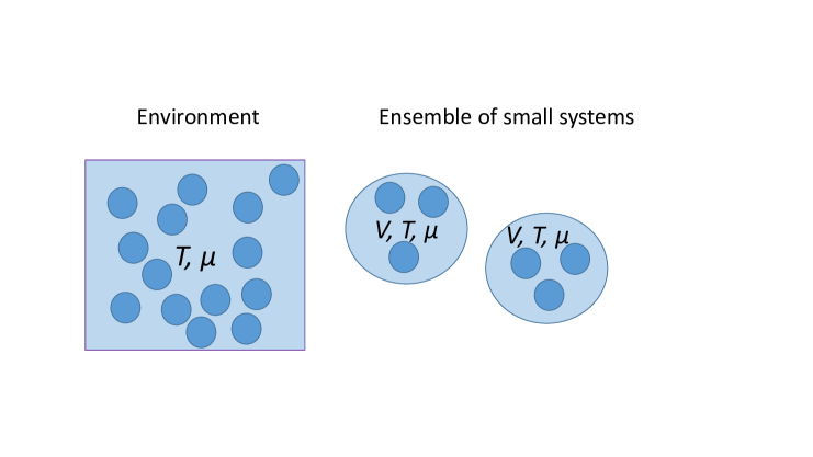
Figure 1: An example of an ensemble of small systems (only two replicas with a volume $V$ are shown) in contact with the environment. The ensemble exchanges energy and mass with the heat- and particle-baths of the environment without being in direct contact.

Using Euler’s theorem of homogeneous functions of degree one, we integrate Eq.1, holding $T$,$V$,$\mu$ and $X$ constant, and obtain

$$U_{t}(T,V,\mu,\mathcal{N})=TS_{t}(T,V,\mu,\mathcal{N})-\hat{p}(T,V,\mu)V\mathcal{N}+\mu N_{t}(T,V,\mu,\mathcal{N})$$ (3)

where we have used the definition $X\equiv-\hat{p}V$. The ensemble averages of internal energy, particle number, and entropy are given by

$$U_{t}(T,V,\mu,\mathcal{N}) \equiv \mathcal{N}U(T,V,\mu)$$

$$N_{t}(T,V,\mu,\mathcal{N}) \equiv \mathcal{N}N(T,V,\mu)$$

$$S_{t}(T,V,\mu,\mathcal{N}) \equiv \mathcal{N}S(T,V,\mu)$$ (4)

While $U\$and $N\$fluctuate because the small systems are open, the entropy does not, and is the same for each ensemble member [4]. By substituting the relations in Eq.4 into Eq.3, we can write the average energy of a single small system as

$$U(T,V,\mu)=TS(T,V,\mu)-\hat{p}(T,V,\mu)V+\mu N(T,V,\mu)$$ (5)

For ease of notation we omit from now the dependence on $T,V,\mu$ and $\mathcal{N}$. In the thermodynamic limit $p=\hat{p}$, and we are left with the classical thermodynamic relation. The last term is necessary in a one-component system because the chemical potential depends on $V,N$.

We obtain the Gibbs relation for the small system by introducing the relations in Eq.4 into Eq.1, using $X\equiv-\hat{p}V$ and Eq.5

$$dU=TdS-pdV+\mu dN$$ (6)

By differentiating Eq.5 and combining the result with Eq.6, the Gibbs-Duhem-like equation becomes

$$d(\hat{p}V)=SdT+pdV+Nd\mu$$ (7)

from which we can derive the following expression for a small system

$$p=\left(\frac{\partial\hat{p}V}{\partial V}\right)_{T,\mu}=\hat{p}+V\left(\frac{\partial\hat{p}}{\partial V}\right)_{T,\mu}$$ (8)

This identity promoted Hill [4] to give the variable $\hat{p}$ the name integral pressure. The variable $p$ was then called the differential pressure. As long as the systems are so small that the integral pressure $\hat{p}$ depends on the volume, the differential pressure $p$ differ from the integral pressure. Expressions similar to Eq.8 apply for $S$ and $N$.

This illustrates the framework developed by Hill [4]; the framework that allows us to systematically handle the thermodynamics of small systems, see the original work for more details.

3 Curvature dependency by Hill’s method

A property that is extensive in the thermodynamic limit can always be written as the sum of this limit plus a small size correction

$$A(T,V,\mu)\equiv a(T,V,\mu)V\equiv a^{\infty}(T,\mu)V+a^{s}(T,\mu,c_{1},c_{2})\Omega$$ (9)

where $a(T,V,\mu)$ is the density of $A(T,V,\mu)$ per unit of volume. In the second equality we used that thermodynamic limit value $a^{\infty}(T,\mu)\equiv A^{\infty}(T,V,\mu)/V$ is independent of the volume. We shall build on the fact that the thermodynamic limit value is uniquely determined, meaning that Eq.9 determines $a^{s}$ uniquely.

The density $a$ and the whole $A$ do not only depend on the size $V$ of the volume, but also on its shape. This dependence was not explicitly indicated in Eqs.1 to 8. The shape-dependence is the reason why there is a small size-correction $a^{s}(T,\mu,c_{1},c_{2})$, which depends on the principle curvatures, $c_{1}\equiv 1/R_{1}$ and $c_{2}\equiv 1/R_{2}$ where $R_{1}$ and $R_{2}$ are the principle radii of curvature of the surface of the small volume. The symbol $\Omega$ is the surface area. The principal curvature of a surface is illustrated for simplicity for a two-dimensional case in Fig.2. The small sphere, touching the wall of the small (ellipsoidal) system, defines the radius of curvature $R_{1}$.

The principle curvatures will generally vary along the surface of a small volume, cf. Fig.2. They are only constant when the system is a sphere or a cylinder. This implies that one should everywhere on the surface use the local values and integrate the corresponding contributions over the surface, see Helfrich [9]. We will here take $c_{1}$ and $c_{2}$ constant, which simplifies the analysis considerably. A generalization to a varying $c_{1}$ and $c_{2}$ can be done, and does not alter the result.

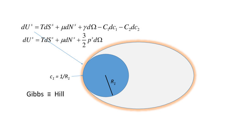
Figure 2: The radius of curvature of a two-dimensional surface (disk). Gibbs thermodynamics for the surface energy is equivalent to Hill’s for a small system.

Eq.9 is valid for $U,S$ and $N$. For the pressures of the volume we have

$$p(T,V,\mu)V = p^{\infty}(T,\mu)V+p^{s}(T,\mu,c_{1},c_{2})\Omega$$

$$\hat{p}(T,V,\mu)V = \hat{p}^{\infty}(T,\mu)V+\hat{p}^{s}(T,\mu,c_{1},c_{2})\Omega$$ (10)

It follows from Eq.10 together with Eq.8 that

$$p^{\infty}(T,\mu)=\hat{p}^{\infty}(T,\mu)$$ (11)

In the thermodynamic limit the small-size corrections are negligible. The Euler equation, Eq.5, becomes using Eq.11

$$u^{\infty}=Ts^{\infty}-p^{\infty}+\mu n^{\infty}$$ (12)

The Gibbs equation, Eq.6, becomes

$$dU^{\infty}=TdS^{\infty}-p^{\infty}dV+\mu dN^{\infty}$$ (13)

By using also Eq.11, Gibbs-Duhem Eq.7 becomes

$$dp^{\infty}=s^{\infty}dT+n^{\infty}d\mu$$ (14)

Not surprisingly these relations have their usual form. This is because they apply to the thermodynamic limit. Subtracting Eq.12 times $V$ from Eq.5 and dividing the result by $\Omega$  we obtain the Euler relation for small-size corrections

$$u^{s}(T,\mu,c_{1},c_{2})=Ts^{s}(T,\mu,c_{1},c_{2})-\hat{p}^{s}(T,\mu,c_{1},c_{2})+\mu n^{s}(T,\mu,c_{1},c_{2})$$ (15)

By subtracting Eq.13 from Eq.6 we obtain for small-size corrections

$$dU^{s}(T,\mu,c_{1},c_{2})=TdS^{s}(T,\mu,c_{1},c_{2})-p^{s}(T,\mu,c_{1},c_{2})\frac{\Omega}{V}dV+\mu dN^{s}(T,\mu,c_{1},c_{2})$$ (16)

From the definitions $L\equiv V^{1/3}$ and $\Omega/V\equiv c_{s}/L$ we have

$$\left(\frac{\partial\Omega}{\partial V}\right)_{T,\mu} = \left(\frac{\partial\Omega}{\partial L}\right)_{T,\mu}\left(\frac{\partial L}{\partial V}\right)_{T,\mu}=\left(2c_{s}L\right)\left(\frac{1}{3L^{2}}\right)=\frac{2}{3}\frac{c_{s}}{L}=\frac{2}{3}\frac{\Omega}{V}$$ (17)

$$\Longrightarrow \frac{\Omega}{V}dV=\frac{3}{2}d\Omega$$

We used as condition that the change of the volume did not imply a change in shape. By substituting the last expression into Eq.16, we obtain Gibbs’ equation that applies when small-size contributions are relevant

$$dU^{s}=TdS^{s}-\frac{3}{2}p^{s}d\Omega+\mu dN^{s}$$ (18)

The Gibbs-Duhem equation for systems with small system corrections similarly becomes

$$d\left(\hat{p}^{s}(T,\mu,c_{1},c_{2})\Omega\right)=S^{s}(T,\mu,c_{1},c_{2})dT+\frac{3}{2}p^{s}(T,\mu,c_{1},c_{2})d\Omega+N^{s}(T,\mu,c_{1},c_{2})d\mu$$ (19)

In order to compare with Gibbs results (below), we use Eq.8 which gives

$$p\left(T,V,\mu\right)=\frac{\partial\hat{p}\left(T,V,\mu\right)V}{\partial V}=\frac{\partial\left(\hat{p}^{\infty}\left(T,\mu\right)V\right)}{\partial V}+\frac{\partial\left(\hat{p}^{s}(T,\mu,c_{1},c_{2})\Omega\right)}{\partial V}$$ (20)

This results in

$$p^{s}\left(T,\mu,c_{1},c_{2}\right)\frac{\Omega}{V}=\hat{p}^{s}(T,\mu,c_{1},c_{2})\frac{\partial\Omega}{\partial V}+\Omega\frac{\partial\hat{p}^{s}(T,\mu,c_{1},c_{2})}{\partial c_{1}}\frac{\partial c_{1}}{\partial V}+\Omega\frac{\partial\hat{p}^{s}(T,\mu,c_{1},c_{2})}{\partial c_{2}}\frac{\partial c_{2}}{\partial V}$$ (21)

Both curvatures change when $V$ changes. As in the derivation of Eq.17  we find

$$\frac{\partial c_{1}}{\partial V}=-\frac{c_{1}}{3V}\text{ \ and \ }\frac{\partial c_{2}}{\partial V}=-\frac{c_{2}}{3V}$$ (22)

Again, the change of the volume did not imply a change in shape. By introducing this equation and Eq.17  we obtain the small system pressure

$$p^{s}\left(T,\mu,c_{1},c_{2}\right)=\frac{2}{3}\hat{p}^{s}(T,\mu,c_{1},c_{2})-\frac{c_{1}}{3}\frac{\partial\hat{p}^{s}(T,\mu,c_{1},c_{2})}{\partial c_{1}}-\frac{c_{2}}{3}\frac{\partial\hat{p}^{s}(T,\mu,c_{1},c_{2})}{\partial c_{2}}$$ (23)

4 Comparing with Gibbs’ results

We are now in a position where we can compare the Euler equation 15 with the one given by Gibbs [7] (see Eq.502 on page 229 of his collected works, volume 1):

$$u^{s}(T,\mu,c_{1},c_{2})=Ts^{s}(T,\mu,c_{1},c_{2})+\gamma(T,\mu,c_{1},c_{2})+\mu n^{s}(T,\mu,c_{1},c_{2})$$ (24)

where $\gamma$ is the common surface tension. It follows that small system pressure can be identified by the surface tension:

$$\gamma(T,\mu,c_{1},c_{2})=-\hat{p}^{s}(T,\mu,c_{1},c_{2})$$ (25)

By introducing this into Eq.23, we obtain for the differential pressure

$$p^{s}\left(T,\mu,c_{1},c_{2}\right)=-\frac{2}{3}\gamma(T,\mu,c_{1},c_{2})+\frac{c_{1}}{3}\frac{\partial\gamma(T,\mu,c_{1},c_{2})}{\partial c_{1}}+\frac{c_{2}}{3}\frac{\partial\gamma(T,\mu,c_{1},c_{2})}{\partial c_{2}}$$ (26)

By using this in the Gibbs relation, we have

$$dU^{s}=TdS^{s}+\gamma d\Omega-\frac{1}{2}\frac{\partial\gamma}{\partial c_{1}}c_{1}d\Omega-\frac{1}{2}\frac{\partial\gamma}{\partial c_{2}}c_{2}d\Omega+\mu dN^{s}$$ (27)

It follows from Eqs.17 and 22 that

$$c_{1}d\Omega=-2\Omega dc_{1}\text{ \ and \ }c_{2}d\Omega=-2\Omega dc_{2}$$ (28)

By introducing this in the Gibbs relation, we obtain

$$dU^{s}(T,\Omega,\mu,c_{1},c_{2})=TdS^{s}(T,\Omega,\mu,c_{1},c_{2})+\gamma(T,\mu,c_{1},c_{2})d\Omega$$

$$+\frac{\partial\gamma(T,\mu,c_{1},c_{2})}{\partial c_{1}}\Omega dc_{1}+\frac{\partial\gamma(T,\mu,c_{1},c_{2})}{\partial c_{2}}\Omega dc_{2}+\mu dN^{s}(T,\Omega,\mu,c_{1},c_{2})$$ (29)

The corresponding Euler relation was already given in Eqs.15 and 24. The Gibbs-Duhem equation, 19, becomes with Eqs.26 and 28

$$d\gamma(T,\mu,c_{1},c_{2}) = -s^{s}(T,\mu,c_{1},c_{2})dT+\frac{\partial\gamma(T,\mu,c_{1},c_{2})}{\partial c_{1}}dc_{1}$$ (30)

$$+\frac{\partial\gamma(T,\mu,c_{1},c_{2})}{\partial c_{2}}dc_{2}-n^{s}(T,\mu,c_{1},c_{2})d\mu$$

The coefficients $C_{1}$ and $C_{2}$ are now identified with

$$C_{1}=\frac{\partial\gamma(T,\mu,c_{1},c_{2})}{\partial c_{1}}\Omega\text{ \ and \ }C_{2}=\frac{\partial\gamma(T,\mu,c_{1},c_{2})}{\partial c_{2}}\Omega$$ (31)

These are identities which follow from Eq.29 as Maxwell relations. By introducing these, we obtain

$$dU^{s}(T,\Omega,\mu,c_{1},c_{2})= TdS^{s}(T,\Omega,\mu,c_{1},c_{2})+\gamma(T,\mu,c_{1},c_{2})d\Omega$$

$$+C_{1}dc_{1}+C_{2}dc_{2}+\mu dN^{s}(T,\Omega,\mu,c_{1},c_{2})$$

Equation 4 is exactly the one given by Gibbs [7] (see Eq.493 on page 225 in his collected works, volume 1) for thermodynamics of surfaces of heterogeneous systems.

5 Concluding remarks

We have seen above that the analysis given by Gibbs [7] of the thermodynamics of heterogeneous systems is equivalent to the thermodynamics of small systems as formulated by Hill [4] 90 years later.

But Hill extended the treatment of small systems much beyond the study of curved surfaces. He used the same ensemble procedure to study, say, adsorption, crystallization, bubbles, all under different environmental conditions. With the equivalence proven, we can take advantage of the broader method of Hill in the study of curved and other surfaces. One of the advantages of Hill’s method is that one obtains the properties of the small system, including surface and curvature contributions without the need to immediately introduce the dividing surface.

It is interesting to note that the small system method, derived from Hill’s basis, gives information on thermodynamic properties of small systems, without having to actually create these small systems. We have earlier demonstrated, using this method, that a scaling law exists, relating surface properties to properties in the thermodynamic limit [13,14]. The important conclusion appears; that information of the surface properties is contained in the characteristic fluctuations of for instance the number of particles and the energy that take place in the small system. This is a very general observation, that also supports the idea that Hill’s thermodynamics may provide a fruitful basis, also for the derivation and use of non-equilibrium thermodynamics for the nano-scale. It is our hope that this can stimulate similar efforts, and lead to a development of non-equilibrium nano-thermodynamics.

Acknowledgment

The authors are grateful to the Research Council of Norway through its Centers of Excellence funding scheme, project number 262644, PoreLab. Discussions with Edgar Blokhuis, Bjørn A. Strøm and Sondre K. Schnell are much appreciated.

References

1. Richardson H. H. et al., Nano Lett. 6 (2006) 783.
2. Govorov A. O. et al., Nanoscale Research Letters 1 (2006) 84.
3. Jain P. K., El-Sayed I. H. and El-Sayed M. A., Nano Today 2 (2007) 18.
4. Hill T. L., Thermodynamics of small systems (Dover, New York) 1994.
5. Hill T. L., Perspective: Nanothermodynamics, Nano Lett. 1 (2001) 111.
6. Latella I., Pérez-Madrid A., Campa A., Casetti L., Ruffo S., Phys. Rev. Lett. 114 (2015) 230601.
7. Gibbs .J W., The Scientific Papers of J. Willard Gibbs, Volume 1, Thermodynamics (Ox Bow Press, Woodbridge, Connecticut) 1993.
8. Tolman R.C., J. Chem. Phys. 17 (1949) 333.
9. Helfrich W., Z. Naturforsch. 28c (1973) 693.
10. Blokhuis E.M. and Bedeaux D., J. Chem. Phys. 95 (1991) 6986.
11. Blokhuis E.M. and Bedeaux D., Physica A 184 (1992) 42.
12. Blokhuis E.M. and Bedeaux D., Heterogeneous Chemistry Reviews, 1 (1994) 55.
13. Strøm B.A., Simon J-M., Schnell S.K., Kjelstrup S., He J., Bedeaux D., PCCP 19 (2017) 9016.
14. Schnell S.K., Vlugt T.J.H., Simon J-M., Bedeaux D., Kjelstrup S., Chem. Phys. Letters 504 (2011) 199.
15. Kjelstrup S. and Bedeaux D., Nonequilibrium Thermodynamics for Heterogeneous Systems, Series on Statistical Mechanics, Vol. 16 (World Scientific, Singapore) 2008.