Covariance constraints for stochastic inverse problems of computer models

Abstract

Stochastic inverse problems are typically encountered when it is wanted to quantify the uncertainty affecting the inputs of computer models. They consist in estimating input distributions from noisy, observable outputs, and such problems are increasingly examined in Bayesian contexts where the targeted inputs are affected by stochastic uncertainties. In this regard, a stochastic input can be qualified as meaningful if it explains most of the output uncertainty. While such inverse problems are characterized by identifiability conditions, constraints of ”signal to noise”, that can formalize this meaningfulness, should be accounted for within the definition of the model, prior to inference. This article investigates the possibility of forcing a solution to be meaningful in the context of parametric uncertainty quantification, through the tools of global sensitivity analysis and information theory (variance, entropy, Fisher information). Such ”forcings” have mainly the nature of constraints placed on the input covariance, and can be made explicit by considering linear or linearizable models. Simulated experiments indicate that, when injected into the modeling process, these constraints can limit the influence of measurement or process noise on the estimation of the input distribution, and let hope for future extensions in a full non-linear framework, for example through the use of linear Gaussian mixtures.

Keywords: inverse problems ;computer models ;stochastic inversion ; Bayesian setting ; sensitivity analysis ; well-posedness ; Fisher information ; entropy ; Sobol’s indices

1 Introduction

Inverse problems appear in many scientific fields, as process engineering, image processing or financial mathematics [37]. In the broadest sense, such problems consist of reconstructing a signal $X$ from indirect observations $Y^{*}$. Many situations consider deterministic linear operators $g$ linking $X$ to $Y^{*}$. Despite this linearity, solving these problems remains usually rather difficult and require regularization methods [17]. These difficulties increase when $g$ is nonlinear, $Y^{*}$ suffers from noise or/and model error $\varepsilon$, and $X$ is stochastic. Such situations frequently occur in the field of uncertainty quantification (UQ) [44], when $X$ is an unknown or weakly known random input vector in $I\!\!R^{p}$, $g:I\!\!R^{p}\to I\!\!R^{q}$ is an implemented (so-called computer) model, and $Y^{*}$ typically comes from sensor or experimental measurements. A common formalization of such problems is assuming

$$Y^{*} = g(X)+\varepsilon$$ (1.1)

where $\varepsilon$ is a stochastic error in $I\!\!R^{q}$, with known probability density function (pdf) $f_{\varepsilon}$. Considering $X$ as random and estimating the features of its pdf $f_{X}$ helps to address the practical concern of accounting for uncertainties surrounding the use of $g$ to perform engineering tasks [24].

Given $f_{\varepsilon}$, the methods for reconstructing (estimating) $f_{X}$ based on an observed sample ${\bf y^{*}_{n}}=(y^{*}_{1},\ldots,y^{*}_{n})$ generally take advantage of the missing data structure of the problem, and use the expectation-maximization (EM) principle in a frequentist setting [18, 7] or alternatively Markov Chains Monte Carlo methods in a Bayesian setting [39, 81, 6, 33] (typically using Gibbs samplers). See [88] for a recent survey of such algorithms and [35, 90, 63] for details on their theoretical convergence properties. While nonparametric frameworks have been extensively studied in the literature [19, 10, 100, 32], several authors in statistical engineering (e.g. [7, 39, 40, 6]) choose to simplify the problem by assuming a multivariate Gaussian input (possibly at the price of a reparametrization)

$$X \sim {\cal{N}}_{p}(\mu,\Gamma)$$ (1.2)

and aim to estimate the mean and covariance $(\mu,\Gamma)\in I\!\!R^{p}\times S^{++}_{p}(I\!\!R)$, where $S^{++}_{p}(I\!\!R)$ is the space of symmetric, positive-definite matrices. The rationale for this practical choice is that the shape of the distribution of $X$ (or a reparametrization of $X$) must obey certain plausibility constraints (e.g., the distribution of a physically-meaning variable may be not multimodal [7, 40]), and to avoid possible difficulties related to a lack of model identifiability, in relation with the size $n$ of ${\bf y^{*}_{n}}$. In order to be verified, the latter can require simplifications of $g$ (e.g., linearization in [18]).

In such settings, however, a few problems may in practice limit the attainment of a solution that is both valid and meaningful. Statistical validity is based on sufficient exploration of the parameter space by the algorithms mentioned above. They have to browse a large number of values of $(\mu,\Gamma)$, and it can occur, for instance, that a Bayesian posterior distribution obtained by sampling under finite computational cost lacks of accuracy and still places importance on implausible values [45]. From a UQ point of view, for many applications it is key to diminish the possibility that a lack of accuracy in the estimation of the distribution of $X$ result in underestimating the input uncertainty (see [54] and [36] for examples in heat transfer and acoustical engineering).

In view of using the model for prediction tasks, we can formalize the notion of a meaningful solution, which is related to the good choice of $g$, by imposing that the pair $(\mu_{i},\Gamma_{i})$ is such that the model

$$Y_{i}=g(X_{i}) X_{i}\sim{\cal{N}}(\mu_{i},\Gamma_{i})$$ with (1.3)

generates plausible values of $Y_{i}$, namely values that remain close to real observations ${\bf y^{*}_{n}}$ and reflect most of their variability. This implies that the underlying phenomenon explaining this variability is globally well reproduced. If this were not the case, it would mean that the error $\varepsilon_{i}\sim f_{\varepsilon}$ distorts the values of $Y_{i}$ to obtain values of $Y^{*}_{i}=Y_{i}+\varepsilon_{i}$ close to ${\bf y^{*}_{n}}$. Hence the model $g$ could probably be improved and should not be used for simulation purpose. Plausibility should therefore be a consequence of the validation of $g$, that ideally helps to ensure that the computational model has sufficiently rigor for the context of use [80]. However, model validation is usually conducted using statistical testing strategies, following a calibration task that estimates particular values of $X$ by minimizing a metric with respect to selected values of $Y^{*}$ (e.g., limit cases) [83, 84]. This leads to validate $g$ only for a selected range of situations, without getting a full guarantee that these situations automatically include the $X_{i}$ generated by (1.3). In a machine learning context where $g$ could be learned from unavailable legacy couples $(x_{j},y_{j})$ (e.g., in situations described in [21] and [69]), this problem amounts to estimating the generalization domain of $X$.

Studying UQ affecting computer models, this problem is of particular concern when $\varepsilon_{i}$ is a mixture of observational noise $\varepsilon_{1}$, approximation error $\varepsilon_{2}$ due to inherent inaccuracies related to discretization [85] and model error $\varepsilon_{3}$. In general, $\varepsilon_{1}$ is known (e.g. through the specifications of the constructor of a measurement system) and $\varepsilon_{2}$ can be bounded [87]. The model error $\varepsilon_{3}$ is often estimated by residual analyses from regression approaches that do not use the generative model $X\sim{\cal{N}}(\mu,\Gamma)$, but rather use selected values of $X$ [98]. This prior estimation diminishes the risk of identifiability issues encountered in stochastic inversion [30]. Especially, such approaches based on designs of numerical experiments are used when $(g,\varepsilon_{3})$ includes a stochastic lower-cost approximation (or meta-model) of a computationally expensive model (e.g., $(g,\varepsilon_{3})$ is chosen as a Gaussian-process based kriging meta-model [4, 39]).

For these reasons, given $g$ and $\varepsilon$, there are possibilities to get meaningless solutions for the inverse problem (1.1-1.2), despite using theoretically appropriate statistical approaches. Restricting ourselves to the unbiased case where the expectation of $\varepsilon$ equals zero, an intuitive way to limit the risks of such solutions is to constrain the search for the values of $\Gamma$ in subspaces of $S^{++}_{p}(I\!\!R)$, by imposing that the variability of $Y^{*}_{i}$ remains mainly explained by the variability of $Y_{i}$, i.e. that of $X_{i}$ ($g$ being deterministic). In terms of global sensitivity analysis (SA ; [28]), this means that an relevant existing solution should be such that a sensitivity indicator of $Y^{*}$ related to $X$ takes values higher than this same sensitivity indicator related to $\varepsilon$. This UQ concern can be interpreted as a supplementary condition to the classical conditions of Hadamard’s well-posed inverse problems: not only a solution should exist, be unique and data-continuously dependent, but it has to be meaningful too. Then constraining $\Gamma$ is similar in spirit to using prior information to transform an ill-posed inverse problem into a well-posed one using regularization techniques [17]. Properly speaking, such a condition is not an identifiability condition, as it does not depend on observable data on its principle (but only sometimes in an indirect way for estimation purpose, as it will be seen further). It should be more understood as a Bayesian prior constraint, helping the statistician to improve the relevance of the forward simulation model for which $(\mu,\Gamma)$ are calibrated.

To our knowledge, this idea was not previously explored in the UQ field, although the need of constraining $\Gamma$ with respect to the covariance of an error was highlighted (but not deeply studied) in [39], precisely when $(g,\varepsilon_{3})$ arises from kriging meta-modeling. The reasons may be that historical approaches to inverse problems in the presence of multiple sources of uncertainty are difficult, still largely based on plug-in estimation [57, 51, 50] to avoid identifiability problems, and that stochastic inversion of highly-dimensional numerical models remains challenging to implement [31, 67].

The objective of this article is therefore to propose a first formalization of the problem of constraining $\Gamma$ with respect to the knowledge of $\varepsilon$, by taking advantage of the SA principles, and to test the interest of this approach to improve the stochastic inversion of a numerical model. Coherently with the previous comment, the Bayesian framework is privileged. The case when $g$ is linear or can be approximated with a linear model is prominent in this article, appearing as a standard framework to study the formalization and impact of these covariance constraints. Indeed, nonlinear simulation models can be well approximated, without the drawbacks of kernel approaches (kernel ad-hoc choice, impossibility of inverting learned mappings [64]), by mixtures of linear models estimated by regression (regression trees being a special form of such meta-models) from a numerical design of experiment (DOE). Recent results obtained in [34, 89, 68] argue for such approaches, which are becoming increasingly competitive from a computational point of view. In this sense, obtaining results with linear or nearly linear models appears as a prerequisite.

More precisely, this article is structured as follows. Main notations and concepts are formally introduced in Section 2. In a preliminary approach, Section 3 studies the case of a linear model $g$ and introduces two simple constraint rules based on well-known SA tools, Sobol’s and entropy-based indices, which provide similar results. A short study is conducted in view of extending these results to locally linearizable models (requiring $g$ being locally differentiable), and illustrates the difficulty of working with such approximations. Then Section 4 provides and studies a general constraining rule, based on Fisher information, in broader settings when $g$ has multidimensional outputs. and can be approximated by a globally linear model in a variational sense. Based on a real case-study previously investigated in the UQ literature, numerical experiments conducted on Section 5 describe how these constraints can be inserted within inversion algorithms and illustrate that they can help to improve the statistical estimation of the distribution of simulated inputs. A discussion section ends this article, opening avenues for future research. Proofs of the stated results are provided in Appendix.

‘

2 Formalism and main notations

Let us introduce here the formalism necessary for the mathematical developments in the following sections. For $p\in I\!\!N^{*}$, $p<\infty$, denote ${\cal{B}}(I\!\!R^{n})$ the Borel $\sigma-$algebra that endows the metric space $(I\!\!R^{p},d)$ where $d$ is induced by the Euclidian norm (generically noted $\|.\|$ along the article, and sometimes $\|.\|_{p}$ to reflect the appropriate dimension and avoid ambiguity).

Let $(I\!\!R^{p},{\cal{B}}(I\!\!R^{p}),\mathbb{P})$ and $(I\!\!R^{q},{\cal{B}}(I\!\!R^{q}),P)$ be two probability spaces, $E=\otimes_{i=1}^{p}E_{i}$ be endowed with a product $\sigma-$algebra and $(X,\varepsilon)$ be two independent random variables from $(I\!\!R^{p},I\!\!R^{q})$ to $(E,I\!\!R^{q})$ in $L^{2}$. Finally, let $g:(E,I\!\!R^{p})\to(I\!\!R^{q},{\cal{B}}(I\!\!R^{q}))$ be in $L^{2}$ and

$$Y = g(X),$$

$$Y^{*} = Y+\varepsilon$$

be two random variables defined on $(I\!\!R^{q},{\cal{B}}(I\!\!R^{q}),P)$. In order to use the classical results of sensitivity analysis, we will also assume that $0<\rm{Var}(Y)<\infty$. Additional assumptions will be introduced later on the differentiability of $g$ when a local linear approximation of $g$ will be studied.

On the basis of this formalism, the problem of stochastic inversion is estimating the unknown $f_{X}$ distribution of $X\in(I\!\!R^{p},{\cal{B}}(I\!\!R^{p}),\mathbb{P})$ from a sample of observations ${\bf y^{*}_{n}}=(y^{*}_{1},\ldots,y^{*}_{n})$ of $Y^{*}$, knowing the pdf $f_{\varepsilon}$ of $\varepsilon\in(I\!\!R^{q},{\cal{B}}(I\!\!R^{q}),P)$. More precisely, choosing a simplifying framework where $f_{\varepsilon}$ and $f_{X}$ are multivariate Gaussian densities, the stochastic inverse problem becomes

Find $$\theta=(\mu,\Gamma)\in I\!\!R^{p}\times S^{++}_{p}(I\!\!R) i\in\{1,\ldots,n\}$$ such that, for :

$$\left\{\begin{array}[]{lll}x_{i}&\sim&{\cal{N}}_{p}(\mu,\Gamma),\\ y^{*}_{i}&=&g(x_{i})+\varepsilon_{i}\end{array}\right.$$ (2.3)

where $$\varepsilon_{1},\ldots,\varepsilon_{n}\overset{\text{\tiny iid}}{\sim}{\cal{N}}_{q}(0,\Sigma) \Sigma\in S^{++}_{q}(I\!\!R)$$ and .

In the remainder of this article, the notation $\theta=(\mu,\Gamma)$ will be often used as the multivariate parameter of interest. Besides, the symbol $|B|$ will be used for denoting the determinant of matrix $B$. If $B$ is a diagonalizable $p\times p$ matrix, denote $\lambda^{B}_{1},\ldots,\lambda^{B}_{p}$ the set of its eigenvalues. Furthermore, we use the notation $I_{q}$ for the unit matrix in $I\!\!R^{q,q}$. Finally, given a set $\{x_{1},\ldots,x_{n}\}$ of real values, denote $x_{\inf}=\min_{1\leq i\leq n}x_{i}$ and $x_{\sup}=\max_{1\leq i\leq n}x_{i}$. Finally, the notation $f\equiv P$ will be used in unambiguous cases to define a probability density function $f$ by its corresponding distribution $P$.

3 A preliminary: Two intuitive notions of meaningful solutions

3.1 Linear models

Under the prism of global sensitivity analysis (GSA ; [91]), the rationale expressed in Introduction can be formalized as follows, starting with the illustrative case of the simple linear model

$$g(x)=a\cdot x\ \ \ \ \text{with $a\in I\!\!R^{q,p}$.}$$ (3.1)

In GSA, the classic notions of variance and entropy play an important role in the comparison of uncertainties incarnated by statistical distributions, that could be intuitively used to express the fact that most of the uncertainty on $Y$ must be explained by the uncertainty on $X$, accounting for possible correlations among the components of $X$, and independence between $X$ and $\varepsilon$. Relevant GSA indices can be chosen as the first-order grouped Sobol’ indices (related to output variance and recalled in Appendix A) and the entropy-based indices proposed by [61] and studied by [73, 3]. Denoting $\mathcal{E}(Y^{*})$ the Shannon-Kullback entropy of $Y^{*}$, the latter stand on the notion of conditional entropy $\mathbb{E}_{X}[\mathcal{E}(Y^{*})|X]$, that indicates the average loss of information on $Y^{*}$ when the behavior of $X$ is known. If $\varepsilon$ is of small influence in the variability of $Y^{*}$, then it can be expected that $\mathbb{E}_{X}\left[\mathcal{E}(Y^{*})|X\right]<\mathbb{E}_{\varepsilon}\left[\mathcal{E}(Y^{*})|\varepsilon\right]$.

From these considerations two definitions can then be derived.

Definition 1.

Let $(S_{X},S_{\varepsilon})$ be the first-order grouped Sobol indices quantifying the uncertainty on $Y^{*}$ explained by $X$ and $\varepsilon$, respectively. Provided $X$ and $\varepsilon$ are independent, the stochastic inverse problem (2.3-3.1) is said to be meaningful in Sobol’ sense if

$$S_{X} > S_{\varepsilon}.$$ (3.2)

Definition 2.

The stochastic inverse problem (2.3-3.1) is said to be meaningful in the entropic sense if

$$\mathbb{E}_{\varepsilon}\left[\mathcal{E}(Y^{*})|\varepsilon\right] > \mathbb{E}_{X}\left[\mathcal{E}(Y^{*})|X\right].$$ (3.3)

Note that the second definition is more general, since Sobol’ indices require that all variances exist. The following proposition straightforwardly provides prior constraints on $\Gamma$ from these two definitions.

Proposition 1.

The stochastic inverse problem (2.3-3.1) is meaningful in Sobol’ sense if and only if

$${\rm{Tr}}(a\Gamma a^{T})>{\rm{Tr}}(\Sigma).$$ (3.4)

It is meaningful in entropic sense if and only if

$$\left|a\Gamma a^{T}\right|>\left|\Sigma\right|.$$ (3.5)

which imposes that $a\Gamma a^{T}$ be invertible.

When the symmetric matrix $a\Gamma a^{T}$ is close to the identity, “the determinant behaves like the trace” [97]: for any bounded matrix $A\in I\!\!R^{q,q}$ and infinitesimal $\varepsilon^{\prime}\in I\!\!R$, denoting $I_{q}$ the unit matrix of rank $q$,

$$|I_{q}+\varepsilon^{\prime}A| = 1+\varepsilon^{\prime}{\rm{Tr}}(A)+O(\varepsilon^{\prime 2}).$$

In such cases (3.4) and (3.5) reflect a similar constraint on $\Gamma$.

Besides, an immediate corollary of Proposition 1 is that both results coincide when the output is univariate.

Corollary 1.

When $q=1$, the stochastic inverse problem (2.3-3.1) is meaningful in Sobol’ and entropic senses if and only if

$$a^{T}\Gamma a > \sigma^{2}.$$ (3.6)

In a Bayesian stochastic inversion framework, an interesting result can be derived, under the additional assumptions that $q=p$ (then (3.5) becomes $\left|a\Gamma a^{T}\right|=|a|^{2}\left|\Gamma\right|$), $a$ be invertible, and that there exists $\beta<\infty$ such that $|\Gamma|<\beta$. Such a constraint is likely to appear in practical applications. For instance, consider that for all $i\in\{1,\ldots,p\}$, $\rm{Var}(X_{i})\leq\beta_{j}$. Then, from Hadamard’s inequality, $\beta=\prod_{i=1}^{p}\beta_{i}$. The following proposition deals with the possibility of handling an integrable Jeffreys measure as a prior for $\Gamma$, and thus providing a practical objective framework for the Bayesian estimation of this covariance matrix. For any parametric density model $f(x|\theta)$ with well-defined Fisher information $I(\theta)$ (see Appendix B for details), Jeffreys’ measure is considered as one of the reference non-informative prior measures on $\theta$ in Bayesian estimation, with rich theoretical properties [22]. Especially, it is invariant through any bijective reparameterisation of $\theta$. Jeffreys’ prior is defined by

$$\pi^{J}(\theta) \propto \sqrt{|I(\theta)|}.$$

However, it is often an improper (non-integrable) measure, which can lead to posterior inconsistencies and paradoxes [55].This is especially the case where no lower bound other than 0 is available for $|\Gamma|$. This result is therefore likely to be useful in contexts of objective Bayesian modeling and selection [9].

Proposition 2.

Assume $q=p$ and $|a|>0$. Let

$$\Omega = \left\{\Gamma\in S^{++}_{p}(I\!\!R)\ ;\ 0<\frac{|\Sigma|}{|a|^{2}}<|\Gamma|<\beta\right\}$$

be the supporting set for the estimation of covariance matrix $\Gamma$ under Definition 2. Let $A$ denote a compact set of $I\!\!R^{p}$. Then Jeffrey’s prior measure for $(\mu,\Gamma)$ in (2.3-3.1), restricted to $A\times\Omega$, is a proper (integrable) probability measure.

3.2 Locally linearizable models

While linear models are generally used in a pure explanatory regression context, one should consider rather, to address more broader situations and examine how to adapt the previous covariance constraints, that $g$ is linearizable in the neighborhood of a given point of interest $x_{0}$. Such a local linearization of $g$ was defended by [7], among others, to avoid prohibitive computational costs in simulation-based inferential algorithms. More generally, local linearization is an usual tool for dealing with inverse problems [96].

Local linearization can be studied using the multivariate first-order Taylor expansion of the vector-valued function $g$ under the assumption that $g$ is Fréchet differentiable in a neighborhood $V_{x_{0}}$ of a given $x_{0}\in I\!\!R^{p}$. More precisely, denote $g^{(i)}$ the $i$th coordinate of $g$ and let $Dg_{x_{0}}=(\frac{\partial g^{(i)}}{\partial x_{j}}(x_{0}))_{i,j}$ be the $(q,p)$ Jacobian matrix of $g$.

H0

: $g:I\!\!R^{p}\to I\!\!R^{q}$ is such that $\forall i\in\{1,\ldots,q\}$, $\forall j\in\{1,\ldots,p\}$, $\frac{\partial g^{(i)}}{\partial x_{i}j}$ exists almost everywhere and $\mathbb{E}\left|\frac{\partial g^{(i)}}{\partial x_{j}}(X)\right|<\infty$ on $V_{x_{0}}$.

Under H0, for any $x\in V_{x_{0}}$, one may write $g(x)=\tilde{g}_{x_{0}}(x)+h_{x_{0}}(x)$ with

$$\tilde{g}_{x_{0}}(x) = g(x_{0})+Dg_{x_{0}}(x-x_{0})\ =\ g(x_{0})+\left(\sum_{j=1}^{p}\dfrac{\partial g^{(i)}}{\partial x_{j}}(x_{0})\left(x_{j}-x_{0_{j}}\right)\right)_{1\leq i\leq q}$$ (3.7)

and $h_{x_{0}}:I\!\!R^{p}\to I\!\!R^{q}$ is a remainder such that $h_{x_{0}}(x)=o\left(\|x-x_{0}\|_{p}\right)$.

Obtaining a constraint on the covariance of $g(X)$ from that of $\tilde{g}_{x_{0}}(X)$ requires modifying the rules (3.4-3.5) by involving quantities related to the geometry of $g(X)$ in $V_{x_{0}}$. In next Proposition we focus on Definition 1 and consider the case of an univariate output $(q=1)$.

Proposition 3.

Assume H0 and $q=1$. Then a sufficient condition for (3.2) is

$${\rm{Tr}}\left[D_{g_{x_{0}}}\Gamma\left(2\mathbb{E}\left[D_{g}(X)\right]-D^{T}_{g_{x_{0}}}\right)\right] \geq {\rm{Tr}}\left[\Sigma\right].$$ (3.8)

Note that when $g(X)=\tilde{g}_{x_{0}}(X)=aX+b$ with $a\in I\!\!R^{q,p}$ and $b\in I\!\!R^{q}$, then $D^{T}_{g_{x_{0}}}=a^{T}$ and (3.8) is exactly the necessary and sufficient condition (3.4). Next example illustrates the fact that (3.8) becomes actually a condition on the full parameter vector $(\mu,\Gamma)$, because of linearization.

Example 1.

Assume $g(x)=1-\exp(-\sum_{i=1}^{p}x_{i})$. Then, around $x_{0}=(0,\ldots,0)$, consider $\tilde{g}_{x_{0}}(x)=\sum_{i=1}^{p}x_{i}$. Denoting $\bar{\mu}=p^{-1}\sum_{i=1}^{p}\mu_{i}$ and $\gamma^{2}=\sum_{i,j}\Gamma_{i,j}$, then $\tilde{g}_{x_{0}}(X)\sim{\cal{N}}(p\bar{\mu},\gamma^{2})$ and $1-g(X)\sim{\cal{LN}}(-p\mu,\gamma^{2})$. With $\mathbb{E}[D_{g}(X)]=\exp(-p\bar{\mu}+\gamma^{2}/2)u^{T}$ and $D_{g_{x_{0}}}=u$ where $u$ is the vector in $I\!\!R^{p}$ such that $u_{i}=1$ for all $i=1,\ldots,p$, then (3.8) becomes

$$\gamma^{2}\left\{2\exp\left(\gamma^{2}/2-p\bar{\mu}\right)-1\right\} \geq {\rm{Tr}}\left[\Sigma\right].$$

Extending the result of Proposition 3 to $q>1$ seems uneasy, although some refinements could probably be derived using trace inequalities (see the remark within the proof). But this is enough to motivate the following comment. Since we only dispose of noisy observations $y^{*}_{1},\ldots,y^{*}_{n}$ of $g(X)+\varepsilon$, estimating consistently $\mathbb{E}[D_{g}(X)]$ or similar functions involving a mean of the Jacobian prior to model inversion appears challenging, if not impossible when $q\neq p$ and $g$ is not an invertible function. Rather, $\mathbb{E}[D_{g}(X)]$ is a function of $\theta=(\mu,\Gamma)$:

$$\mathbb{E}\left[D_{g}(X)\right] = \int_{I\!\!R^{p}}D_{g}(x)f_{X}(x|\theta)\ dx$$

and (3.8) should be inserted as a constraint on $\Theta$ within the stochastic inversion algorithms evoked hereinbefore. For each candidate $\theta_{i}$ in such routines, the integral above has to be computed numerically (e.g., by Monte Carlo batch sampling or gradient descent techniques). Even in the case where $g$ can be automatically differentiated, it is likely that the rejection rate of candidates $\theta_{i},\theta_{i+1},\ldots$ will make the computational cost prohibitive. For this reason, variational linear approximation will be studied later in the article, instead of local linearization, as it involves the first and second-order moments of the distribution of $g(X)$, which can be consistently estimated from the available observations.

4 Fisher inversion constraints

The intuitive notion of a meaningful inverse problem proposed in Definition 1 is based on first-order hierarchising of conditional variances. This appears somewhat limited to reflect how input uncertainty from $X$ or $\varepsilon$ is transmitted to the observed output $Y^{*}$. Since information can be viewed as a reduction of uncertainty [23], the main concepts of classical information theory [25] appear useful in providing a broader framework for analysis and well formalized means for characterizing the effects of uncertainty. Because the inverse problem is to estimate $\theta=(\mu,\Gamma)$, using a truly parametric measure of information seems more appropriate. The most usual measure of information is Fisher information [25]. See Appendix B for a technical reminder and details about its interpretation.

4.1 Formalisation

Under the conditions of existence (cf. Appendix B), denote by $I_{g(X)}(\theta)\in S^{+}_{q}(I\!\!R)$ and $I_{Y^{*}}(\theta)\in S^{+}_{q}(I\!\!R)$ the Fisher information matrices provided respectively by $g(X)$ and $Y^{*}$ about $\theta$. Since the impact of $\varepsilon$ is to degrade information, it can be expected that $I_{g(X)}(\theta)$ be greater than $I_{Y^{*}}(\theta)$, according to some order relation $\succeq$ defined for symmetric matrices. The Loewner order appears as the most natural candidate for $\succeq$, as it is the partial order induced by the translations over the convex cone of positive semi-definite matrices. It is frequently used to define monotone functions over this cone and has important equivalence relations and implications with other order relations [5, 49]. It is therefore expected that

$$I_{g(X)}(\theta) \succeq I_{Y^{*}}(\theta)$$ (4.1)

where $A\succeq B$, for two squared matrices $A$ and $B$, means that $A-B$ is a positive semidefinite matrix.

Stating that most of information on $\theta$ in $Y^{*}$ is transmitted from $g(X)$ implies that the difference between $I_{g(X)}(\theta)$ and $I_{Y^{*}}(\theta)$, which is a measure of the information loss because of the noise $\varepsilon$, should not be greater than a fraction $(1-1/c)I_{g(X)}(\theta)$ where $c>1$. Therefore we propose the following definition.

Definition 3.

For $c>1$, the stochastic inverse problem is meaningful in Fisher’ sense if

$$I_{g(X)}(\theta)\succeq I_{Y^{*}}(\theta)\succeq\dfrac{1}{c}I_{g(X)}(\theta).$$ (4.2)

An intuitive value for $c$ is 2, but further developments will show that $c$ can be related to important concepts in matrix inversion and signal processing, as linear system conditioning and signal over noise ratio. This can help to assess its value in practice, and it will be shown that the choice $c=4$ allows to make the Fisher and Sobol’ constraints equivalent in simple situations.

The following sections consider several usual situations encountered in stochastic inversion and provide necessary conditions (NC), sufficient conditions (SC) and necessary and sufficient conditions (NSC) on the features of the covariance $\Gamma$ of $X$ such that (4.2) be verified. In practice, NC and NSC should be preferred to SC, as the latter correspond to prior constraints on $\Gamma$ that threaten to overestimate how $X$ varies.

4.2 Gaussian linear models

We assume a linear $g:x\mapsto Hx$, with $H\in\mathbb{R}^{q,p}$ of full rank. Besides we assume $\Sigma\in S^{++}_{q}(I\!\!R)$. By abuse of notation, we denote in next equations $\partial/\partial\mu$ and $\partial/\partial\Gamma$ the differentiations of functions of $\theta=(\mu,\Gamma)$ with respect to the free components of $\theta$. We remind that if $A$ is real square matrix such that $A\succeq 0$, then $\lambda^{A}_{\sup}=\|A\|_{2}$ the Euclidian norm.

4.2.1 Fisher matrix characterization

In order to provide useful conditions for (4.2), we first provide a characterization of the Fisher matrix for the Gaussian model

$$Y_{\alpha} =HX+\alpha\varepsilon\ \ \ \text{with $\alpha\in\{0,1\}$,}$$ (4.3)

that encompasses the cases $Y_{0}=Y$ and $Y_{1}=Y^{*}$. Assuming $\Sigma\in S^{++}_{q}(I\!\!R)$, we denote

$$\Psi_{\alpha}(\Gamma) = \Sigma^{-\alpha/2}H\Gamma H^{T}\Sigma^{-\alpha/2}$$

(with the convention $\Sigma^{0}=I_{q}$), which can be seen as a multivariate generalization of the signal over noise ratio (MSNR) characterizing (4.3) ; see [26] for details on this concept widely used in signal processing and the characterization of channel features.

Theorem 1.

Denote $I_{{Y}_{\alpha}}(\theta)$ the Fisher information matrix for (4.3), assuming $\theta=(\mu,\Gamma)\in I\!\!R^{p}\times S^{++}_{p}(I\!\!R)$. Let ${\partial^{2}}/{\partial\Gamma^{2}}$ indicate the double differentiation with respect to the free components of $\Gamma$. Then, assuming that $\alpha I_{q}+\Psi_{\alpha}(\Gamma)$ is inversible,

$$I_{{Y}_{\alpha}}(\theta) = \left(\begin{array}[]{ll}I_{{Y}_{\alpha}}(\mu)&{\bf 0}\\ {\bf 0}&I_{{Y}_{\alpha}}(\Gamma)\end{array}\right)$$

where

$$I_{{Y}_{\alpha}}(\mu) = H^{T}\Sigma^{-\alpha/2}\left(\alpha I_{q}+\Psi_{\alpha}(\Gamma)\right)^{-1}\Sigma^{-\alpha/2}H,$$

$$I_{{Y}_{\alpha}}(\Gamma) = -\dfrac{1}{2}\sum\limits_{i=1}^{q}\dfrac{\partial^{2}}{\partial\Gamma^{2}}\log\left(\alpha+\lambda^{\Psi_{\alpha}(\Gamma)}_{i}\right).$$ (4.5)

Next proposition and its corollaries provide more refined results for the Fisher submatrices in the frequent situation where $\Gamma$ is chosen to be diagonal. It highlights the role of the eigenvalues of the MSNR in the information matrix. It requires to introduce the semidefinite matrices $H_{k}=[h_{i,k}]^{T}_{1\leq i\leq q}$ and

$$\tilde{A}_{k,\alpha} = \Sigma^{-\alpha/2}H_{k}H^{T}_{k}\Sigma^{-\alpha/2}$$ (4.6)

that play a key role in the characterization of this Fisher matrix.

Proposition 4.

Assume $\Gamma=diag(\tau^{2}_{1},\ldots,\tau^{2}_{p})$ and $\theta=(\mu,\Gamma)\in I\!\!R^{p}\times S^{++}_{p}(I\!\!R)$. Denote $V^{\Gamma}_{\alpha}=(v_{\alpha,1},\ldots,v_{\alpha,q})$ an orthonormal basis of $(q,1)-$eigenvectors for $\Psi_{\alpha}(\Gamma)$, and define

$$\nu^{\alpha}_{i,k}=v^{T}_{\alpha,i}\tilde{A}_{k,\alpha}v_{\alpha,i} \eta^{\alpha}_{i,k,l}=v^{T}_{\alpha,i}\tilde{A}_{l,\alpha}\Psi^{+}_{i}(\Gamma)\tilde{A}_{k,\alpha}v_{\alpha,i}$$ and

where $\Psi_{i}(\Gamma)=\lambda^{\Psi_{\alpha}(\Gamma)}_{i}I_{q}-\Psi_{\alpha}(\Gamma)$ and $A^{+}$ is the generalized Moore-Penrose pseudo-inverse of $A$. Then

$$I_{{Y}_{\alpha}}(\mu) = H^{T}\Sigma^{-\alpha/2}\left(\alpha I_{q}+\sum\limits_{k=1}^{p}\tau^{2}_{k}\tilde{A}_{k}\right)^{-1}\Sigma^{-\alpha/2}H,$$ (4.7)

and $\forall(k,l)\in\{1,\ldots,p\}^{2}$, the $(k,l)-$term of matrix $I_{{Y}_{\alpha}}(\Gamma)$ is

$$I_{{Y}_{\alpha}}(\Gamma)_{k,l} = \dfrac{1}{2}\sum\limits_{i=1}^{q}\left\{\frac{\nu^{\alpha}_{i,k}\nu^{\alpha}_{i,l}}{\left(\alpha+\lambda_{i}^{\Psi_{\alpha}(\Gamma)}\right)^{2}}-\frac{\eta^{\alpha}_{i,k,l}+\eta^{\alpha}_{i,l,k}}{\alpha+\lambda_{i}^{\Psi_{\alpha}(\Gamma)}}\right\}.$$ (4.8)

Next corollary assumes that each outer product $H_{k}H^{T}_{l}$ is symmetric, for all couples $(k,l)\in\{1,\ldots,p\}$. It is verified when $q=1$ (univariate output), when $p=1$ (univariate input, since $H_{k}=H_{l}$) or more generally when the rank of $H$ is $1$. In the special case where $p=q$ and $H$ is a diagonal matrix, then it is easy to see that $H_{k}H^{T}_{l}$ is symmetric too.

Corollary 2.

Assume $\Gamma=diag(\tau^{2}_{1},\ldots,\tau^{2}_{p})$ and $\theta=(\mu,\Gamma)\in I\!\!R^{p}\times S^{++}_{p}(I\!\!R)$. Assume furthermore that $\Sigma$ is diagonal and $H_{k}H^{T}_{l}$ is symmetric for all couples $(k,l)\in\{1,\ldots,p\}^{2}$. Denote $\Lambda_{{\alpha}}=(\|\Sigma^{-\alpha/2}H_{1}\|^{2}_{2},\ldots,\|\Sigma^{-\alpha/2}H_{p}\|^{2}_{2})^{T}$ and $\tilde{\Lambda}_{{\alpha}}=diag\Lambda_{{\alpha}}$. Then

$$I_{{Y}_{\alpha}}(\Gamma) = \frac{\Lambda_{{\alpha}}\Lambda^{T}_{{\alpha}}}{2\left(\alpha+{\rm{Tr}}\left(\tilde{\Lambda}_{\alpha}\Gamma\right)\right)^{2}}.$$ (4.9)

Without the assumption of a diagonal $\Sigma$, Corollary 3 provides a last but useful result deriving straightforwardly from Theorem 1, assuming $\Gamma=\tau^{2}I_{p}$ (hence ${\partial^{2}}/{\partial\Gamma^{2}}={\partial^{2}}/{\partial(\tau^{2})^{2}}$).

Corollary 3.

Assume $\Gamma=\tau^{2}I_{p}$ and $\theta=(\mu,\tau^{2})\in I\!\!R^{p}\times I\!\!R_{+*}$. Then $\Psi_{\alpha}(\Gamma)=\tau^{2}\Psi_{\alpha}$ with $\Psi_{\alpha}=\Sigma^{-\alpha/2}HH^{T}\Sigma^{-\alpha/2}$ and

$$I_{{Y}_{\alpha}}(\mu) = H^{T}\Sigma^{-\alpha/2}\left(\alpha I_{q}+\tau^{2}\Psi_{\alpha}\right)^{-1}\Sigma^{-\alpha/2}H,$$

$$I_{{Y}_{\alpha}}(\Gamma) = \dfrac{1}{2}\sum\limits_{i=1}^{q}\left(\frac{\lambda^{\Psi_{\alpha}}}{\alpha+\tau^{2}\lambda^{\Psi_{\alpha}}}\right)^{2}.$$

4.2.2 Conditions for Fisher constraints

From the previous results, some conditions for (4.2) can be derived. Note first that, from Theorem 1,

$$I_{g(X)}(\theta)-I_{Y^{*}}(\theta) = \left(\begin{array}[]{ll}I_{Y_{0}}(\mu)-I_{Y_{1}}(\mu)&{\bf 0}\\ {\bf 0}&I_{Y_{0}}(\Gamma)-I_{Y_{1}}(\Gamma)\end{array}\right)$$

$$-\frac{1}{c}I_{g(X)}(\theta)+I_{Y^{*}}(\theta) = \left(\begin{array}[]{ll}I_{Y_{1}}(\mu)-\frac{1}{c}I_{Y_{0}}(\mu)&{\bf 0}\\ {\bf 0}&I_{Y_{1}}(\Gamma)-\frac{1}{c}I_{Y_{0}}(\Gamma)\end{array}\right).$$

Then (4.2) is true if and only if the following conditions are simultaneously verified:

$$I_{Y_{0}}(\mu) \succeq I_{Y_{1}}(\mu),$$ (4.12)

$$I_{Y_{0}}(\Gamma) \succeq I_{Y_{1}}(\Gamma),$$ (4.13)

$$I_{Y_{1}}(\mu) \succeq \frac{1}{c}I_{Y_{0}}(\mu),$$ (4.14)

$$I_{Y_{1}}(\Gamma) \succeq \frac{1}{c}I_{Y_{0}}(\Gamma).$$ (4.15)

Hence necessary conditions (NC) for any of these inequalities are NC for (4.2). In the following results, we always assume that $H\Gamma H^{T}$ and $\Sigma$ are invertible. The result provided in Proposition 4 highlights the difficulty of obtaining necessary and sufficient conditions (NCS) for (4.2) in general cases, as they would require NCS for differences of sums of products of orthonormal vectors that belong to different spaces, as well as prior knowledge on the ordering of pseudo-inverse matrices. For this reason, several common simplified situations are examined in the following, in particular situations when the output $Y$ is unidimensional.

Proposition 5.

Inequation (4.12) is always true.

Comparing $I_{Y_{0}}(\Gamma)$ and $I_{Y_{1}}(\Gamma)$ under the context of Proposition 4 can be simplified if $\Psi_{0}(\Gamma)$ and $\Sigma^{1/2}$ are co-diagonalizable (namely if they share a common base of diagonalization). Especially, this is true if $\Sigma=\sigma^{2}I_{q}$ or if $q=1$.

Proposition 6.

Assume that $\Gamma$ is diagonal and $\Psi_{0}(\Gamma)=HH^{T}$ and $\Sigma^{1/2}$ are co-diagonalizable. Then Inequation (4.13) is true.

In other situations, with $q>1$ and $\Gamma$ still diagonal, denote $Y_{[i]}$ the $i$th-dimensional output of $Y\in I\!\!R^{q}$. Considering only this output dimension, then $I_{{Y_{[i]}}_{0}}(\Gamma)\succeq I_{{Y_{[i]}}_{1}}(\Gamma)$. Note besides that (4.5) and (4.8) in Theorem 1 and Proposition 4 highlight the fact that, provided $\Sigma=\sigma^{2}I_{q}$, then

$$I_{Y_{\alpha}}(\Gamma) = \sum\limits_{i=1}^{q}I_{{Y_{[i]}}_{\alpha}}(\Gamma).$$

Consequently, by transitivity of the Loewner order, the relation (4.13) still hold when $\Sigma=\sigma^{2}I_{q}$.

Proposition 7.

Inequation (4.14) is true if and only if

$$H\Gamma H^{T} \succeq \frac{1}{c-1}\Sigma.$$ (4.16)

Furthermore, a NC for (4.14) is

$$\|\Gamma\|_{2} \geq \frac{1}{c-1}\left\|(HH^{T})^{-1}\Sigma\right\|_{2}.$$ (4.17)

Note that this last result is actually a NC for (4.16), and it can be easily transformed into a sufficient condition (SC) for this latter inequation by replacing $\|\Gamma\|_{2}=\lambda^{\Gamma}_{\sup}$ by $\lambda^{\Gamma}_{\inf}$ (see the proof).

Proposition 8.

Assume the conditions and notations of Corollary 2. Denote $\rho=\sqrt{\left\|\left(\Lambda_{1}\Lambda^{T}_{1}\right)^{+}\left(\Lambda_{0}\Lambda^{T}_{0}\right)\right\|_{2}}$, $\gamma=\|\Sigma^{-1/2}\|^{4}_{2}\|\Lambda_{1}\|^{-2}_{2}\|\Lambda_{0}\|^{2}_{2}$ and $U=\sqrt{c}\tilde{\Delta}_{0}-\rho\tilde{\Delta}_{1}$. Then Inequation (4.15) is true if and only if

$${\rm{Tr}}(U\Gamma) \geq \rho$$ (4.18)

and if $c>\gamma^{2}$ a NC (resp. SC) for (4.18) is

$$\|\Gamma\|_{2}\ \ \ \ \text{({resp.} $\tau^{2}_{\inf}$)} \geq \frac{\rho}{\sqrt{c}\|\Lambda_{0}\|^{2}_{2}-\rho\|\Lambda_{1}\|^{2}_{2}}.$$

The case $\Gamma=\tau^{2}I_{p}$.

Studying this simplistic situation allows to provide a clear rationale to select a value for $c$, allowing to connect the Sobol’ and entropy-based constrained problems previously studied with the Fisher-based constrained problem. From Corollary 3 one may derive the following results.

Proposition 9.

Assume $\Gamma=\tau^{2}I_{p}$ and $\theta=(\mu,\tau^{2})\in I\!\!R^{p}\times I\!\!R_{+*}$. Denote $\Psi_{\alpha}=\Sigma^{-\alpha/2}HH^{T}\Sigma^{-\alpha/2}$. Then a NC for (4.2) is

$$\tau^{2} \geq \frac{1}{\sqrt{c}-1}\|\Psi_{1}\|^{-1}_{2}.$$ (4.19)

Condition (4.19) refines the general NC (4.17), noticing that $\|\Psi_{1}\|^{-1}_{2}=\left\|(HH^{T})^{-1}\Sigma\right\|_{2}$ when $HH^{T}$ and $\Sigma^{1/2}$ are co-diagonalizable. Expression (4.19) highlights a lower bound for the signal over noise ratio (MSNR ; see $\S$ 4.2.1): necessarily,

MSNR $$= \tau^{2}\|\Psi_{1}\|_{2}\ \geq\ \frac{1}{\sqrt{c}-1}.$$

It seems reasonable a priori to assume $\text{MSNR}\geq 1$ to define a meaningful inverse problem (namely, the information required for the inversion task is not overwhelmed by the noise – including model error), which leads to select $c$ such that

$$c\geq 4.$$ (4.20)

This lower bound for $c$ seems to make sense if we go back to Section 3. Consider the example given by (3.1), where $q=1$ and $H=a\in\mathbb{R}$; then Condition (4.19) gives $(\sqrt{c}-1)\tau^{2}>{\sigma^{2}}/{a^{2}}$. For model (3.6), where $q=1$ and $H=a\in\mathbb{R}^{p}$, this gives $(\sqrt{c}-1)\tau^{2}>{\sigma^{2}}/{\parallel a\parallel^{2}}$. Choosing $c=4$, the conditions provided for Sobol’ or entropic senses are recovered: $\tau^{2}\|a\|^{2}_{2}\geq\sigma^{2}$. In the context of Proposition 8, if $q=1$ and $c=4$, then $\rho=\sigma^{2}$, $\gamma=1$ and the NSC (4.18) similarly becomes $\tau^{2}\geq\frac{\sigma^{2}}{\|a\|^{2}_{2}}$.

4.3 Gaussian linearizable models

4.3.1 Theoretical approximation

Let us go back to the more general case where $g$ is some deterministic function from $\mathbb{R}^{p}$ to $\mathbb{R}^{q}$, not necessarily linear. For nonlinear models, the intractability of the likelihood function carries forward to the calculation of the Fisher information matrix, preventing us from establishing directly simple NC for Condition (4.2). A commonly used approach to bypass this problem is to linearize the regression function. Consequently, $Y$ is still assumed to have its first and second order moments finite.

To avoid the technical difficulties raised by local linearity (see $\S$ 3.2), consider now that $g$ can be linearizable in a variational sense, at least on a given domain of interest. In the context of this study, such an approximation – replacing the output $Y$ by an approximation $\tilde{Y}$ – should be considered relevant if it allows to carry the most part of information transferred by $g$. For this reason, the error resulting from the approximation should have a small impact on $\tilde{Y}$. Intuitively, this means that obtaining a Fisher constraint from the linearized model should help the inversion of the nonlinear model, which requires statistical estimation; this heuristic will be tested in practice in Section 5.

More formally, an information-theoretic rationale, usual in variational analysis, can be invoked to define $\tilde{Y}$ as the best approximation of $Y$ in a distributional sense using the Kullback-Leibler divergence to quantify the quality of the approximation [25]. Recall that this divergence between two distributions $P$ and $Q$, with respective pdf $(f_{p},f_{q})$ that are absolutely continuous with respect to each other on a common support $D$, is given by

$$\text{KL}\left(P\|Q\right)=\int_{D}f_{p}(x)\log\frac{f_{p}(x)}{f_{q}(x)}dx.$$

Proposition 10.

Denote $Y=g(X)$ and $Y^{*}=Y+\varepsilon$ with $\mathbb{E}[\varepsilon]=0$ and $X\sim{\cal{N}}_{p}(\mu,\Gamma)$ with $\Gamma\in S^{++}_{p}(I\!\!R)$. Denote ${\cal{L}}_{p,q}$ the space of homoscedastic Gaussian linear models from $I\!\!R^{p}$ to $I\!\!R^{q}$ and assume $q\leq p$. Define $U\sim{\cal{N}}(0,S)$ with $S$ independent of $X$ and for any $H\in I\!\!R^{q,p}$, define in ${\cal{L}}_{p,q}$ the linear model

$$\tilde{Y} = H(X-\mu)+\mathbb{E}[Y^{*}]+U.$$

Assume $\mbox{Cov}(Y^{*})\succeq\Sigma+S$ and denote $(f_{Y},f_{\tilde{Y}_{H}})$ the pdf of $(Y,\tilde{Y})$, respectively. Then there exists $H^{*}\in I\!\!R^{q,p}$ such that

$$f_{\tilde{Y}_{H}^{*}} = \arg\min\limits_{f\in{\cal{L}}_{p,q}}\text{KL}\left(f_{Y},f\right)$$

and $H^{*}$ is such that $H^{*}\Gamma H^{*T}+S=\mbox{Cov}(Y^{*})-\Sigma$.

It follows from this last result, adapting Proposition 7, that a NC for a meaningful linear approximation is

$$H^{*}\Gamma H^{*T} = \mbox{Cov}(Y^{*})-\Sigma-S\ \succeq\ \frac{1}{c-1}\left(\Sigma+S\right)$$

or similarly

$$\mbox{Cov}(Y^{*}) \succeq \frac{c}{c-1}\left(\Sigma+S\right).$$ (4.21)

Since $A\succeq B\Rightarrow{\rm{Tr}}(A)\succeq{\rm{Tr}}(B)$ for $(A,B)$ two square matrices, this implies directly the following result.

Proposition 11.

A NC for a meaningful linear approximation of $g$ is

$${\rm{Tr}}\left(H^{*}\Gamma H^{*T}\right) \geq \frac{1}{c-1}{\rm{Tr}}\left(\Sigma+S\right).$$ (4.22)

In the case where $\Gamma=\tau^{2}I_{p}$, estimating $H^{*}$ appears useless to provide a condition on $\tau^{2}$, as stated by next Corollary.

Corollary 4.

Assume $\Gamma=\tau^{2}I_{p}$. Then a NC for the linear approximation is (4.19), replacing $\Psi_{1}$ by

$$\Psi = \left(\Sigma+S\right)^{-1/2}\left(\mbox{Cov}(Y^{*})-S-\Sigma\right)\left(\Sigma+S\right)^{-1/2}.$$ (4.23)

4.3.2 Computational aspects

The previous results require to get consistent estimators of $\mathbb{E}[Y^{*}]$ and $\mbox{Cov}(Y^{*})$. In this stochastic inversion context, since a sample of noisy observations $(y^{*}_{i})_{1\leq i\leq n}$ is always available in practice, it can be used to compute the usual empirical estimators $(\bar{y}^{*}_{n},{c}^{*}_{n})$

$$\bar{y}^{*}_{n} = \frac{1}{n}\sum\limits_{i=1}^{n}{y}^{*}_{i},$$ (4.24)

$$\bar{c}^{*}_{n} = \frac{1}{n}\sum\limits_{i=1}^{n}\left({y}^{*}_{i}-\bar{y}^{*}_{n}\right)\left({y}^{*}_{i}-\bar{y}^{*}_{n}\right)^{T}.$$ (4.25)

While $H$ is not required for the computation of (4.23), $S$ must be estimated too. Since this covariance matrix expresses the error between $g$ and the best linear model, a simple approach to estimating $S$ can be based on using a numerical Design Of Experiments (DOE), or training sample, $({x}^{\prime}_{j},{y}^{{}^{\prime}}_{j}=g({x}^{\prime}_{j}))_{1\leq j\leq m}$ with $x^{\prime}_{j}=(x^{\prime}_{j,l})_{1\leq l\leq p}$ and $y^{\prime}_{j}=(y^{\prime}_{j,t})_{1\leq t\leq q}$, an usual tool for the preliminary exploration of computer models.

The choice of a DOE is part of an usual and general problem in numerical analysis of computer models, that depends on both the computational easiness of sampling with $g$ and the dimension of $X$. To avoid defining formal bounds on the numerical support of $X$, in a Bayesian informative setting where a prior $\theta\sim\pi(\theta)$ is assumed to be known, sampling uniformly the DOE within the highest predictive prior density region $\{X;\ X\sim{\cal{F}}(\theta),\ \theta\sim\pi(\theta)\}$ is intuitive. But very generally, space-filling type approaches with projection regularity properties on subspaces of the sampling space, such as the maximin Latin Hypercube sampling, are preferred to avoid clusters and filling gaps. They require bounded domains that may be defined using extreme quantiles of the predictive prior density. See [29] for more details.

The availability of the DOE allows to understand $S$ as the covariance of residuals in a multiple regression, consistently estimated by

$${s}^{*}_{n,m} = \left(W^{\prime}_{m,n}-X^{\prime}_{m}\hat{H}_{n,m}\right)\left(W^{\prime}_{m,n}-X^{\prime}_{m}\hat{H}_{n,m}\right)^{T}$$ (4.26)

where $W^{\prime}_{m,n}\in I\!\!R^{m,q}$ and its $(i,j)$-element is $y^{\prime}_{i,j}-\bar{y}^{*}_{n,j}$, $X^{\prime}_{m}\in I\!\!R^{m,p}$ and $\hat{H}_{n,m}\in I\!\!R^{p,q}$ solves the normal equation of the associated linear system, namely

$$\hat{H}_{n,m} = \left(X^{{}^{\prime}T}_{m}X^{\prime}_{m}\right)^{-1}X^{{}^{\prime}T}_{m}W^{\prime}_{m,n}$$ (4.27)

provided the DOE allows $X^{{}^{\prime}T}_{m}X^{\prime}_{m}$ to be invertible. Note that this approach has sense only if the resulting approximation of the left term of (4.23) is positive definite, hence if

$$c^{*}_{n}-{s}^{*}_{n,m} \succ \Sigma.$$ (4.28)

5 Numerical experiments

5.1 General framework

This section illustrates the effect of constraining the variance of $X$ in an usual Bayesian setting. Consider the stochastic inverse problem (2.3) and the general prior form advocated in [39] and [40]:

$$\mu|\Gamma \sim {\cal{N}}_{p}\left(\mu_{0},\Gamma/\alpha\right),$$ (5.1)

$$\Gamma \sim \mathcal{IW}_{p}(\Upsilon,\nu).$$ (5.2)

where $\mathcal{IW}$ denotes the inverse Wishart distribution on $S^{++}_{p}(I\!\!R)$, and where the prior hyperparameters $(\mu_{0},\alpha,\Upsilon,\nu)$ are fixed. This choice is often made for conjugacy reasons. Indeed, given an observed sample $\mathbf{y}^{*}=(y^{*}_{1},\ldots,y^{*}_{n})$, a Gibbs sampler adapted from [39] is a natural approach to generate samples from the posterior distribution $\pi(\mu,\Gamma|y^{*}_{1},\ldots,y^{*}_{n})$ [99], that implements a data augmentation scheme and benefit from conditional form stability. Given initializing values $(\mu^{[0]},\Gamma^{[0]})$ for the parameters, and initialized values $\mathbf{X}^{[0]}$ for the missing variables $\mathbf{X}=(X_{1},\ldots,X_{n})$, generate the following Markov chain for $r=0,1,2,\dots$:

 

$$\text{1.}\ \ \Gamma^{[r+1]} \sim \mathcal{IW}_{p}\left(\Upsilon+\sum_{i=1}^{n}(\mu^{[r]}-X_{i}^{[r]})(\mu^{[r]}-X_{i}^{[r]})^{T}+\alpha(\mu^{[r]}-\mu_{0})\times\right.$$ (5.4)

$$\ \hskip 28.45274pt\left.(\mu^{[r]}-\mu_{0})^{T},\,\nu+n+1\right),$$

$$\text{2.}\ \ \mu^{[r+1]} \sim \mathcal{N}_{p}\Big{(}\frac{\alpha}{n+\alpha}\mu_{0}+\frac{n}{n+\alpha}\overline{\mathbf{X}_{n}^{[r]}},\,\frac{\Gamma^{[r+1]}}{n+\alpha}\Big{)}\ \ \text{ with $\overline{\mathbf{X}_{n}^{[r]}}=\frac{1}{n}\sum\limits_{i=1}^{n}X_{i}^{[r]}$},$$

$$\text{3.}\ \ \mathbf{X}^{[r+1]} \sim \tilde{\pi}\left(\mathbf{X}^{[r+1]}|g,\mathbf{y}^{*},\Sigma,\mu^{[r+1]},\Gamma^{[r+1]}\right),$$

this latter conditional density being proportional to

$$\exp\Big{\{}-\frac{1}{2}\sum_{i=1}^{n}\Big{[}\left(X^{[r+1]}_{i}-\mu^{[r+1]}\right)^{T}\left(\Gamma^{[r+1]}\right)^{-1}\left(X^{[r+1]}_{i}-\mu^{[r+1]}\right)$$

$$+\left(y^{*}_{i}-g(X^{[r+1]}_{i})\right)^{T}\Sigma^{-1}\left(y^{*}_{i}-g(X^{[r+1]}_{i})\right)\Big{]}\Big{\}}$$ (5.5)

 

Since (5.5) does not belong to a closed form family of density functions, a Metropolis-Hasting (MH) step can be used to simulate $\mathbf{X}^{[r+1]}$ from its full conditional distribution [99]. Following the advices of [39] resulting from many numerical tests, a multivariate random walk sampling candidates $\mathbf{X}_{n}^{[r]}$ can be an efficient instrumental distribution for this MH step. An additional gain of choosing the prior (5.1-5.2) is that the meaning of hyperparameters $(\mu_{0},\alpha,\Upsilon,\nu)$ is straightforward, as described in [40].

5.2 Motivating case-study

In this later article, the authors considered a hydraulic engineering model $g(X,d)$ previously used in [8] where $d$ is a known water discharge value of a river, $X$ is a unknown, two-dimensional vector of roughness coefficients for the riverbed and floodplain, respectively, and $Y$ is the corresponding bivariate vector of water heights (levels) in each part of the geographical area. A simplified (while rather good) approximation of $g$ is the following:

$$Y=\left(X_{2}+\left(\dfrac{d\cdot\sqrt{5000}}{300\cdot\sqrt{55-X_{2}}}\cdot X_{1}\right)^{0.6},\dfrac{d^{\ 0.4}\cdot X_{1}^{0.6}\cdot(55-X_{2})^{0.3}}{300^{0.4}\cdot 5000^{0.3}}\right).$$ (5.6)

In the remainder of this section, numerical experiments are conducted to compare the matching between the posterior predictive distribution of the missing values $X$ computed using the previous algorithm with a chosen simulation distribution, in settings where the prior (5.2) is constrained or not by the condition $\Gamma\in\Omega^{(k)}_{j}$ ($j\in\{A,B,C\}$). “Constrained by” means that Step 1 of the algorithm is replaced by a MH step where:

• the instrumental distribution for $\Gamma$ is proportional to

  $$\mathcal{IW}_{p}\left(\Upsilon+\sum_{i=1}^{n}(\mu^{[r]}-X_{i}^{[r]})(\mu^{[r]}-X_{i}^{[r]})^{T}+\alpha(\mu^{[r]}-\mu_{0})\times\right.$$

  $$\ \hskip 85.35826pt\left.(\mu^{[r]}-\mu_{0})^{T},\,\nu+n+1\right)\mathbbm{1}_{\left\{\Gamma\in\Omega^{(k)}_{j}\right\}},$$

  which can be simulated by simple acceptation-rejection;

• the Metropolis ratio does not involve the constraint $\mathbbm{1}_{\left\{\Gamma\in\Omega^{(k)}_{j}\right\}}$.

This appears necessary since, with $\Gamma\in\Omega^{(k)}_{j}$, the conditional posterior of $\Gamma$ given the other parameters is no longer an Inverse Wishart distribution. It is likely that best sampling techniques can be used, but they were not investigated in this article.

The simulation data $X$ are generated according to $f_{s}(X)\equiv{\cal{N}}(\mu_{s},\Gamma_{s})$ where $\mu_{s}=(30,50)$ and $\Gamma_{s}={diag}(5^{2},1)$, while several values of $d$ are considered, sampled from $f_{d}\equiv\text{Gumbel}(1013,100)$, that define several instances of $g$. Such choices lead to physically plausible observable values

$$Y^{(k)*}_{i} = g\left(X_{i},d^{(k)}_{i}\right)+\varepsilon_{i},\ \ \ \text{$i\in\{1,\ldots,n\}$, $k\in\{1,\ldots,M\}$,}$$ (5.6)

in a real context where the model is used to invert roughness coefficients of a French river [40]. Following the magnitudes provided by these authors, the covariance matrix of noise $\varepsilon$ is chosen as $\Sigma={diag}(1^{2},0.1^{2})$ and the chosen prior hyperparameters for (5.1-5.2) are summarized on Table 1.

Table 1: Prior hyperparameters.

$\mu_{0}$	(35, 49)
$\alpha$	1
$\nu$	5
$\Upsilon$	$2\begin{pmatrix}7.5^{2}&0\\ 0&1.5^{2}\end{pmatrix}$

5.3 Models and prior constraints

In this framework where $g$ is not linear, a class of $M$ simplified linear models $\hat{g}^{(1)},\ldots,\hat{g}^{(M)}$, or surrogates approximating $g$ was produced as follows, for the experimental needs. Following approaches advised by [52] in a broader framework of Gaussian meta-modelling, a maximin Latin Hypercube design of $N=2700$ values of $X$ was sampled within the cubic domain ${\cal{A}}=[20,50]\times[30,60]$ instead of a quasi-uniform one, and the corresponding values $Y^{(k)}=g(X,d^{(k)})$ were computed, given a sampled value of $d^{(k)}\sim f_{d}$, for $k\in\{1,\ldots,M\}$ with $M=200$. $M$ multivariate linear (surrogate) models were fitted from the $M\times N$ couples $(x^{(k)}_{i},y^{*(k)}_{i})_{i,k}$, such that

$$y^{*(k)}_{i} = \hat{g}_{M}(x^{(k)}_{i})+\varepsilon_{i},$$

$$\hat{g}_{M}(x^{(k)}_{i}) = y^{(k)}_{i}+u^{(k)}_{i}\ =\ a^{(k)}x^{(k)}_{i}+b^{(k)}+u^{(k)}_{i}$$ (5.8)

where each $u^{(k)}_{i}$ was estimated as the bivariate centered Gaussian noise ${\cal{N}}(0,S^{(k)})$, approximating the model error between $g$ and $\hat{g}^{(k)}$, where each $S^{(k)}$ is estimated from (4.26), with

$$\bar{y}^{(k)*}_{n}\simeq\left(\begin{array}[]{l}52.13\\ 1.76\end{array}\right) \bar{c}^{(k)*}_{n}\simeq\left(\begin{array}[]{ll}2.6&-0.14\\ -0.14&0.038\end{array}\right).$$ and

Details on computations and diagnostics are provided in Appendix D.1. On average, the sum of $\Sigma$ and $S^{(k)}$ was found to be

$$\mathbb{E}\left[\Sigma+S^{(k)}\right] = \begin{pmatrix}1.008&-0.003\\ -0.003&0.012\end{pmatrix}$$

while the average values of matrix $a^{(k)}$ and vector of intercepts $b^{(k)}$ are, respectively

$$\mathbb{E}\left[a^{(k)}\right] = \begin{pmatrix}0.03&0.029\\ 1.10&-0.064\end{pmatrix}\ \ \ \ \ \text{and}\ \ \ \mathbb{E}\left[b^{(k)}\right]\ =\ \left(\begin{array}[]{l}-2.53\\ 3.88\end{array}\right).$$

For the $M$ models, it was checked that $\left|\Sigma\right|=0.01\leq\left|\Sigma+S^{(k)}\right|\sim 0.012\leq\left|a^{(k)}\Gamma_{s}a^{(k)T}\right|\sim 0.027$, ie. the uncertainty in $X$ is of primary influence in the uncertainty in $Y$, according to the entropy-based notion of uncertainty expressed by Definition (2). Roughly speaking, each linear surrogate transmits a signal that is not overwhelmed by the noise. Besides, empirical condition (4.28) was respected for all simulated samples, with

$$\left|\bar{c}^{(k)*}_{n}-\Sigma-S^{(k)}\right| > 0.01.$$

Finally, two situations of stochastic inversion are studied:

Situation 1.

We focus only on inverting the roughness coefficient from the water level on the riverbed, namely the first dimension of $Y$ (named $Y_{[1]}$), as collecting regular observations $Y^{*}_{[1]}$ is the most traditional approach to feed such hydraulic problems. Then relevant constraints for $\Gamma$ arise from considering $q=1$.

Situation 2.

We focus on solving the inverse problem considering the whole set of two-dimensional observations.

Then, several constraints on $\Gamma$, associated to $g$ or to each $\hat{g}^{(k)}$ are now defined for the experiments. They simply take the form of indicator constraints for defining the supporting subset of $S^{++}_{p}(I\!\!R)$ for $\Gamma$ in (5.2). For all $k\in\{1,\ldots,M\}$, consider:

$$\Omega^{(k)}_{A}\left(\Sigma\right) = \left\{\Gamma\in S^{++}_{p}(I\!\!R),\ \left|a^{(k)}\Gamma a^{(k)T}\right|\geq\left|\Sigma\right|\right\},$$

$$\Omega^{(k)}_{B} = \Omega^{(k)}_{A}\left(\Sigma+S^{(k)}\right),$$

$$\Omega^{(k)}_{C} = \left\{\Gamma\in S^{++}_{p}(I\!\!R),\ \|\Gamma\|_{2}\geq\frac{1}{3}\left\|\left(a^{(k)}a^{(k)T}\right)^{-1}\Sigma\right\|_{2}\right\},$$

$$\Omega^{(k)}_{D} = \left\{\Gamma\in S^{++}_{p}(I\!\!R),\ \rm{Tr}\left(\left(2\tilde{\Delta}^{(k)}_{0}-\rho^{(k)}\tilde{\Delta}^{(k)}_{1}\right)\Gamma\right)\geq\rho^{(k)}\right\},$$

$$\Omega^{(k)}_{E} = \left\{\Gamma\in S^{++}_{p}(I\!\!R),\ {\rm{Tr}}\left(a^{(k)}a^{(k)T}\right)\geq\frac{1}{3}{\rm{Tr}}\left(\Sigma+S^{(k)}\right)\right\}.$$

Domain $\Omega^{(k)}_{A}$ appears as a soft entropic prior constraint on $\Gamma$ coming from (3.5), that assumes negligible model error with respect to a linear surrogate. It can be rightfully tested over models $\hat{g}^{(k)}$ and $g$. Domain $\Omega^{(k)}_{B}$ is a more stringent condition that accounts for this model error, that should be tested over model $g$ only. Domain $\Omega^{(k)}_{C}$ comes from (4.16), using $c=4$. It is appropriate for linear surrogates $\hat{g}^{(k)}$ but it can be tested too over model $g$. Domain $\Omega^{(k)}_{D}$, coming from (4.18) with $c=4$, can be tested in a similar way but only makes sense in Situation 1 (univariate output of interest), replacing $\Sigma$ by its first diagonal component $\Sigma_{[1,1]}$. The composite constraint $\Omega^{(k)}_{C}\cap\Omega^{(k)}_{D}$ can be also be rightfully tested in Situation 1. Finally, $\Omega^{(k)}_{E}$ comes from (4.22) with $c=4$ and is applicable only on model $g$. Tested models with their prior domains (or indicator constraints) for $\Gamma$ are summarized on Table 2.

Table 2: Models and associated prior covariance constraints tested.

Indicator	Models	Prior domain	Output dimensionality $q$ used for inversion
	Linear surrogates
$L_{1}$	$\hat{g}^{(k)}(X)$	$S^{++}_{p}(I\!\!R)$ (no prior constraint)	$q\in\{1,2\}$
$L_{2}$	$\hat{g}^{(k)}(X)$	$\Omega^{(k)}_{A}(\Sigma)$	$q\in\{1,2\}$
$L_{3}$	$\hat{g}^{(k)}(X)$	$\Omega^{(k)}_{C}$	$q\in\{1,2\}$
$L_{4}$	$\hat{g}^{(k)}(X)$	$\Omega^{(k)}_{D}$	$q=1$
$L_{5}$	$\hat{g}^{(k)}(X)$	$\Omega^{(k)}_{C}\cap\Omega^{(k)}_{D}$	$q=1$
	Nonlinear models
$T_{1}$	$g\left(X,d^{(k)}\right)$	$S^{++}_{p}(I\!\!R)$ (no prior constraint)	$q\in\{1,2\}$
$T_{2}$	$g\left(X,d^{(k)}\right)$	$\Omega^{(k)}_{A}(\Sigma)$	$q\in\{1,2\}$
$T_{3}$	$g\left(X,d^{(k)}\right)$	$\Omega^{(k)}_{B}$	$q\in\{1,2\}$
$T_{4}$	$g\left(X,d^{(k)}\right)$	$\Omega^{(k)}_{C}$	$q\in\{1,2\}$
$T_{5}$	$g\left(X,d^{(k)}\right)$	$\Omega^{(k)}_{D}$	$q=1$
$T_{6}$	$g\left(X,d^{(k)}\right)$	$\Omega^{(k)}_{C}\cap\Omega^{(k)}_{D}$	$q=1$
$T_{7}$	$g\left(X,d^{(k)}\right)$	$\Omega^{(k)}_{E}$	$q\in\{1,2\}$

5.4 Experiments

For $k\in\{1,\ldots,M=200\}$, a $n-$sample $Y^{(k)}$ of vectors is generated from (5.6). For each sample and each couple of model and prior constraints, an instance of the Metropolis-Hastings-within-Gibbs (or hybrid Gibbs) algorithm described in $\S$ 5.1 is run, adding each prior indicator constraint for $\Gamma$ to the simulation step (5.4). Three Markov chains are run in parallel for each scenario, and the convergence towards each stationary, marginal posterior distribution of $X$ is assessed by satisfying the usual condition on Gelman’s statistic $\hat{R}_{G}<1.02$ [13] (more details are provided on Appendix E). Convergence is usually observed from 6000 iterations and chains are run such that, after a decorrelation step, posterior samples contain 5000 vectors.

By design in [40], the prior remains weakly informative and in agreement with the generated data (in the sense of [12]). The ability of the algorithm to estimate correctly the parameters, as well as the effect of constraints to shrink the highest posterior regions around the true values, can be appreciated on Figure 2 for Situation 1 ($q=1$) and Figure 2 for Situation 2 ($q=2$). While these figures show that these effects may be non-negligible (both on $\mu$ and $\Gamma$ through their entanglement in the estimation algorithm), their impact on the relevance of the posterior predictive distribution of $X$ can be more finely addressed as follows. Each marginal posterior on $X$, denoted by its density function $f_{S_{j}}(x|\hat{y}^{*(k)},d^{(k)})$ where $S\in\{L,T\}$ and $i\in\{1,\ldots,6\}$, provides an approximation of the simulation distribution $f_{S}$, and it can be compared to other posteriors through error indicators $e_{S_{j}}$ defined with respect to this latter distribution. The Kullback-Leibler divergence between the simulation distribution $f_{s}(X)$ and each marginal posterior is used here for defining this indicator:

$$e^{(k)}_{S_{j}} = KL\left(f_{s}(.)\|f_{S_{j}}(.|\hat{y}^{*(k)},d)\right),$$

$$= -H(f_{s})-\mathbb{E}_{f_{s}}\left[\log f_{S_{j}}(.|\hat{y}^{*(k)},d)\right]$$

where $H(f_{s})$ is the entropy of $f_{s}$, provided by (C.1). The second term is estimated by Monte Carlo: for a large value $Q=100,000$,

$$\mathbb{E}_{f_{s}}\left[\log f_{S_{j}}(.|\hat{y}^{*(k)},d)\right] \simeq \frac{1}{Q}\sum\limits_{l=1}^{Q}\log\hat{f}_{S_{j}}(x_{j}|\hat{y}^{*(k)},d_{k})$$

where $x_{j}\overset{iid}{\sim}f_{s}$ and $\hat{f}_{S_{j}}$ is a two-dimensional Gaussian-kernel density estimator of ${f}_{S_{j}}$ defined from posterior sampling, defined on the bounded domain ${\cal{A}}$.

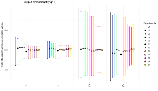
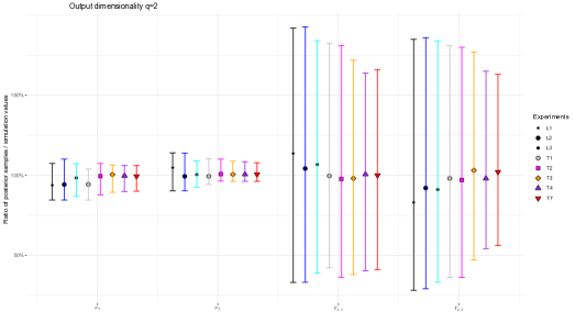
Figure 1: Summary of posterior relative means and 90% credibility intervals with respect to simulation values, on average on the values of $d$, for $n=30$. The inversion algorithm considers Situation 1 ($q=1$). Means are perfect estimates of simulation values when the $y-$axis values reach 100%.

Figure 2: Summary of posterior relative means and 90% credibility intervals with respect to simulation values, on average on the values of $d$, for $n=30$. The inversion algorithm considers Situation 2 ($q=2$). Means are perfect estimates of simulation values when the $y-$axis values reach 100%.

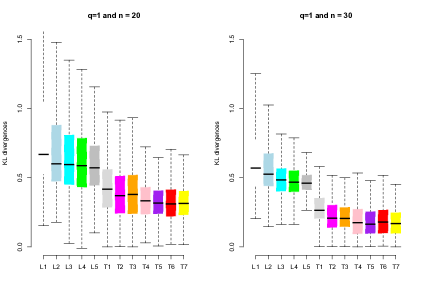
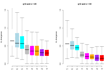
Figure 3: Boxplots of errors $e^{(k)}_{S_{j}}$ (KL divergences) between classes of models and the simulation model (Situation 1: $q=1$), for two different data sizes.

Figure 4: Boxplots of errors $e^{(k)}_{S_{j}}$ (KL divergences) between classes of models and the simulation model (Situation 2: $q=2$), for two different data sizes.

Boxplots summarizing how the errors $e^{(k)}_{S_{j}}$ are distributed are displayed on Figures 4 and 4 . As it could be expected, the posterior distributions estimated from the linear surrogates (L1 to L5) have a larger error relative to the target distribution than the posterior distributions produced from the sampling model. When the dimension of output observations increases (from Situation 1 to Situation 2), posterior predictive distributions appear slightly closer to the true simulation distribution, as it could be expected again. Since all linear surrogates $\hat{g}^{(k)}$ are well defined according to (3.5), and because it accounts for model error in the prior constraint, it was expected that the posterior $L_{3}$ be closer to the simulation distribution ${\cal{N}}(\mu_{s},\Gamma_{s})$ than $L_{1}$ and $L_{2}$. This behavior can scarcely be observed on these plots, because of the weakness of this error. While the proximity of any posterior based on linearity approximation with the target distribution diminishes with the size $n$, it can nevertheless be observed that, on this example, the constraints build from linear approximations improve the separation of signal and noise within the stochastic inversion algorithm when it involves the true sampling model. The constraint resulting from a variational approximation seems to be as effective as the other constraints, while the latter are not completely relevant for all situations. More generally, on this example inserting prior constraints help on average getting better recovery of the predictive posterior distribution and producing posterior estimates that fit better with the features of the underlying true distribution of $X$.

6 Discussion

Based on common concepts of sensitivity analysis of numerical models, this article proposes and studies a notion of meaningful solution to a stochastic inverse problem involving noisy observations or model error, commonly encountered in situations involving linearizable computer models or linear operators. This notion is related to the context of uncertainty quantification and crudely says that an input solution is meaningful if its distribution transmit more uncertainties to the output than other sources of uncertainties, as model error or/and observational noise. In the chosen parametric framework, using linear or linearizable models, the comparison of Fisher information matrices, based on the intuition (4.1), seems an appropriate choice, as it can constrain the main features of the input distribution with respect to those of the combination of observational noises and model errors. Thus, the necessary or sufficient constraints obtained are either minimum bounds on the features of the input covariance. In practice, this type of constraint makes it possible to limit the size of the search space for a solution to the inverse problem. First experiments on toy case studies have shown that this approach can result in an improvement of the inversion task. These results highlight the need to rely on a simultaneous call for real observations and a numerical design of experiment to inform the geometry of the numerical model, in order to produce exploitable constraints for stochastic inversion. This first work seems to us to be a useful starting point to produce constraint rules derived both from theory and from the knowledge of numerical experiments, which raises interesting design problems.

Several results linking quantities usually encountered in numerical conditioning problems were obtained, which allows us to suppose that there exist deep connections between the proposed prior constraints and classical algebraic tools encountered in the treatment of ill-posed regression problems. Strong links certainly also exist between these prior constraints and the regularization terms needed to solve the latter (as described in Introduction), which can indeed be described as Bayesian penalties for regression problems. While it is necessary that these preliminary results must continue to be numerically tested, beyond the case study considered in this article, we therefore hope that they will pave the way for further studies on these connections between domains. They seem to carry important stakes in the context of the increasing use of numerical models.

In this sense, it seems particularly relevant to study connections with other subdomains of global sensitivity anaysis, related to the use of other well-established indices as Borgonovo’s moment-independent indices [11], Shapley values [86], Hilbert-Schmidt sensitivity indices (HSIC ; [27]) or, in a more inclusive way, probabilistic sensitivity measures recently defined by [2]. The authors of this last publication also define a non-parametric Bayesian framework for the estimation of such indices. Its interest is to improve how taking account of uncertainty on the estimation of these indices in situations where the number of simulations of the real model is limited. Insofar as the implementation of our methodology necessarily relies on the estimation of uncertainty indicators, and that the computational cost is a practical fact of inverse problems, the control of the estimation error should encourage us to involve it in the construction of the rules that we proposed to define what could be a meaningful problem. The work carried out by will thus be a source of inspiration for future research in this direction, and improvement of our approach.

Among the other issues to address, One of the first issues is obviously the extension of these results to non-Gaussian situations and non-linear models, as well as the relaxation of theoretical hypotheses. Some structural choices could be modified in the variational analysis in $\S$ 4.3. Beyond the Gaussian case, moment matching resulting from minimizing the inclusive KL divergence occurs for some other exponential distributions, the von Mises-Fisher distribution on the unit sphere, and close mechanisms were recently found for some hyperspherical distributions (see [62] and references therein). Furthermore, it is likely that some results can besides be improved by using necessary conditions based on powerful trace inequalities. Moreover, recent advances in connecting matrix partial ordering and statistical applications, highlighted by [46], could certainly help to extend the results presented in this article. And above all, as we introduced earlier, the use of linear models can feed approximation approaches based on Gaussian mixtures of linear models. Through a preliminary exploration of the properties of the $g$ model, using a numerical design of experiment to choose carefully, variational approaches based on linear regression mixtures could be investigated. Note that it is likely that a more general class of divergences, as the $\alpha-$divergences proposed by [78], could lead to tractable results.

Notice however that the approximation of complex models with linear surrogates is today one of the most popular avenues for discussing the interpretability of these complex models [48]. This type of approach has developed strongly in the field of machine learning and deep learning, where model interpretability is an important prerequisite for the industrialization of these models. This is evidenced by the considerable development of LIME techniques [43]. Nevertheless, it goes without saying that the error, or proximity, between a complex model and its linear surrogate must itself be interpretable [1], and that the linear surrogate must be inferred in such a way as to ensure the reproduction of the major part of the signal. In this sense, we believe that our results can contribute to improve this type of procedure.

Another stake concerns the link between the Bayesian approach to uncertainty and meta-modeling. Beyond the Bayesian benefits described in Proposition 2, we think besides that this approach may be developed to provide rules of selecting covariance kernel structures in the frequent situation when $g$ is considered continuous and second-order stationary but is computationally costly, then replaced by a kriging Gaussian process $\hat{g}$, to which is added a second (zero-mean) Gaussian process as a prior on the so-called discrepancy of $\hat{g}$ with respect to $g$. This additive process tries to capture correlation effects visible in the residuals that cannot be identified in a white Gaussian noise. The inference of such meta-models, introduced by [57], was studied by numerous authors (see [16, 102] for recent reviews) working in the field of uncertainty quantification. It is intuitive, for identifiability reasons, that the additional discrepancy (meta)model should provide more contrasted values with respect to $\hat{g}$ than $\hat{g}$ with $g$ [15], and this can be interpreted as a reasonable prior constraint of the nature of the two covariance kernels. Nonetheless, to our knowledge no formal rule still exist for this elicitation, but only rules of thumb based on the experience of researchers.

Continuing with the statistical estimation itself, two technical aspects could be examined more carefully. First, the choice of covariance estimators used in this article could certainly be improved, using shrinkage techniques [66, 20]. Second, the algorithmic acceleration of MCMC approaches exploring the space of the relevant covariance matrices ($\S$ 5.1) is an interesting topic since these numerical techniques are expensive by definition. Beyond the hybridization of the Metropolis and Gibbs techniques, two research avenues seem to us relevant for this purpose: improving the choice of instrumental distributions supported on the intersection of the cone of semidefinite positive matrices with subspaces of $\Theta$ generated by the constraints, and adapting recent techniques based on Langevin dynamics and the exploration of highly-dimensional settings [81, 82].

Finally, other approaches of stochastic inversion, listed in particular in [94], could also be studied from the point of view proposed in this article, and adapted. Especially, spectral approaches such as polynomial chaos expansion [65, 104] offer calculation facilities to hierarchize uncertainties. Besides, the choice of Fisher information is limited to models for which it is at least not singular ; distributional approaches to sensitivity, as those based on Bregman divergences [27], could help to define broader methodologies with fewer assumptions.

Appendix A Grouped Sobol’s indices

Closed Sobol’s indices [93], based on Hoeffding’s decomposition and the independence of all input variables, are one the most common indicators used in global sensitivity analysis of computer models. In the present situation we are interested by hierarchising the importance of two groups of input variables $X$ and $\varepsilon$ in the variance of output $Y^{*}=\hat{g}(Z)$ where $Z=(X,\varepsilon))\in I\!\!R^{p}\times I\!\!R^{q}$ and $\hat{g}(Z)=g(X)+\varepsilon$. Each group of variables can contain dependent components but we assume that $X$ and $\varepsilon$ are independent. In this case, when $Y^{*}$ is univariate, so-called first-order grouped Sobol’s indices, defined by [53] and later studied by [14], generalize usual Sobol’s indices:

$$S_{X}=\frac{\rm{Var}[\mathbb{E}[Y^{*}|X]]}{\rm{Var}[Y^{*}]} S_{\varepsilon}=\frac{\rm{Var}[\mathbb{E}[Y^{*}|\epsilon]]}{\rm{Var}[Y^{*}]}.$$ and (A.1)

Other generalizations focus on the marginal output effects of each correlated input component in $Z$ (e.g., [76]). The notion of first order is related to the fact that $S_{X}$ and $S_{\varepsilon}$ do not measure the (second-order) impact of the interactions between $X$ and $\varepsilon$ to the output $Y^{*}$ [14].

More generally, when $Y^{*}$ is multidimensional, indices (A.1) were extended by [41] and [42] under the strong hypothesis that the components of $Z$ are independent. Hoeffding’s decomposition of $\tilde{g}$, assuming this independence between the $Z_{i}$, leads to write an expansion of the following form [92]

$$\tilde{g}(Z) = c+\tilde{g}_{\bf u}(Z_{\bf u})+\tilde{g}_{/\bf u}(Z_{/\bf u})+\tilde{g}_{\bf u,/\bf u}(Z_{\bf u},Z_{/\bf u})$$

where ${\bf u}$ is any non-empty subset of ${\bf d}=\{1,\ldots,p+q\}$, $Z_{\bf u}=(Z_{i},i\in{\bf u})$ and $Z_{/\bf u}=(Z_{i},i\in{\bf d}/{\bf u})$, $c=\mathbb{E}[Y^{*}]$ and

$$\tilde{g}_{\bf u} = \mathbb{E}[Y^{*}|Z_{\bf u}]-c,$$

$$\tilde{g}_{/\bf u} = \mathbb{E}[Y^{*}|Z_{/\bf u}]-c,$$

$$\tilde{g}_{\bf u,/\bf u} = Y^{*}-\tilde{g}_{\bf u}-\tilde{g}_{/\bf u}-c.$$

Thanks to $L^{2}$-orthogonality,

$${\mbox{Cov}[Y^{*}]} = {\mbox{Cov}[\tilde{g}_{\bf u}(Z_{\bf u})]}+{\mbox{Cov}[\tilde{g}_{/\bf u}(Z_{/\bf u})]}+{\mbox{Cov}[\tilde{g}_{\bf u,/\bf u}(Z_{\bf u},Z_{/\bf u})]},$$ (A.2)

then the multivariate first-order grouped Sobol’s indices [42] are defined by

$$S_{\bf u} = \frac{{\rm{Tr}}\left(I_{q}\mbox{Cov}[\tilde{g}_{\bf u}(Z_{\bf u})]\right)}{{\rm{Tr}}\left(I_{q}\mbox{Cov}[Y^{*}]\right)}.$$ (A.3)

In the specific case of model (2.3-3.1), under the assumption of intern dependencies among the $X_{i}$ but since $g(X)$ is independent on $\varepsilon$, then

$${\mbox{Cov}[Y^{*}]} = {\mbox{Cov}[g(X)]}+{\mbox{Cov}[\varepsilon]}.$$ (A.4)

Then Equation (A.2) still holds with $\tilde{g}_{\bf u}(Z_{\bf u})=g(X)$, $\tilde{g}_{/\bf u}(Z_{/\bf u})=\varepsilon$ and $\tilde{g}_{\bf u,/\bf u}(Z_{\bf u},Z_{/\bf u})=0$, then the use of indices (A.3) remains appropriate, their meaning being preserved.

Appendix B The Fisher information

The Fisher information $I_{X}(\theta)$ is a measure of the amount of information that an observable random variable $X$ carries about an unknown parameter $\theta\in\mathbb{R}$ upon which the probability of $X$ depends. This key statistical concept can help to quantify the uncertainty of a model or alternatively the amount of information carried by a model [74]. Especially, let us recall that $I_{X}(\theta)$ can be explained by a local differentiation of Shannon’s entropy in the space of probability distributions, through the De Bruijn’s identity [95]. If there exists no minimal set of necessary regularity conditions per se for the existence of $I_{X}(\theta)$, most authors agree on the following sufficient conditions of existence, positivity and continuity in an subset of $\Theta$ (see for instance [47], $\S$ 3.4): let $f(X;\theta)$ be the probability density/mass of $X$ conditional on the value of $\theta$. This function must be absolutely continuous in $\theta$ and the derivative ${\partial}f(x;\theta)/{\partial\theta}$ must exist for almost all $x$.

Then

$$I_{X}(\theta)=\mathbb{E}\left[\left(\dfrac{\partial}{\partial\theta}\ln f(X,\theta)\right)^{2}\right]=\int\left(\dfrac{\partial}{\partial\theta}\ln f(X,\theta)\right)^{2}f(x,\theta)dx$$

or alternatively, if $\ln f(x,\theta)$ is twice differentiable with respect to $\theta$ and under some regularity conditions, as

$$I_{X}(\theta)=-\mathbb{E}\left[\dfrac{\partial^{2}\ln f(X,\theta)}{\partial\theta^{2}}\right].$$

Similarly, if $\theta=(\theta_{1},...,\theta_{N})\in\mathbb{R}^{N}$, the Fisher Information matrix $I_{X}(\theta)\in\mathbb{R}^{N\times N}$ is defined as

$$\left(I_{X}(\theta)\right)_{ij}=-\mathbb{E}\left[\dfrac{\partial^{2}\ln f(X,\theta)}{\partial\theta_{i}\theta_{j}}\right].$$

In the Gaussian case, where $X\sim\mathcal{N}_{p}\left(\mu(\theta),\Gamma(\theta)\right)$ and $\theta=(\theta_{1},...,\theta_{N})$, $\mu(\theta)=\left(\mu_{1}(\theta),...,\mu_{p}(\theta)\right)$, $\Sigma(\theta)=\left(\Gamma_{ij}(\theta)\right)_{1\leq i,j\leq p}$ ,

$$\left(I_{X}(\theta)\right)_{ij}=\dfrac{\partial\mu(\theta)^{T}}{\partial\theta_{i}}\Gamma(\theta)^{-1}\dfrac{\partial\mu(\theta)}{\partial\theta_{j}}+\dfrac{1}{2}\textrm{Tr}\left(\Gamma(\theta)^{-1}\dfrac{\partial\Gamma(\theta)}{\partial\theta_{i}}\Gamma(\theta)^{-1}\dfrac{\partial\Gamma(\theta)}{\partial\theta_{j}}\right)$$ (B.1)

for all $1\leq i,j\leq N$.

If the mean and the covariance depend on two different parameters $\alpha\in\mathbb{R}^{l}$ and $\beta\in\mathbb{R}^{m}$, i.e $\theta:=(\alpha,\beta)$ and $X\sim\mathcal{N}_{p}(\mu(\alpha),\Gamma(\beta))$, then, using the Slepian-Bangs (SB) compact formula for the Fisher information matrix of a multivariate Gaussian distribution [56] (Appendix 3C),

$$I_{X}(\theta) = diag(I^{(1)}_{\alpha,\beta},I^{(2)}_{\beta})$$

where

$$\left(I^{(1)}_{\alpha,\beta}\right)_{1\leq i,j\leq l}=\dfrac{\partial\mu(\alpha)^{T}}{\partial\alpha_{i}}\Sigma(\beta)^{-1}\dfrac{\partial\mu(\alpha)}{\partial\alpha_{j}}$$

and

$$\left(I^{(2)}_{\beta}\right)_{1\leq i,j\leq m} = \dfrac{1}{2}\textrm{Tr}\left(\Sigma(\beta)^{-1}\dfrac{\partial\Sigma(\beta)}{\partial\beta_{i}}\Sigma(\beta)^{-1}\dfrac{\partial\Sigma(\beta)}{\partial\beta_{j}}\right).$$ (B.2)

Appendix C Proofs

Proof of Proposition 1.

From Definition 1, Equation (A.4) and for the model considered in (2.3-3.1),

$$S_{X}=\dfrac{{\rm{Tr}}\left(\mbox{Cov}\left[Y\right]\right)}{{\rm{Tr}}\left(\mbox{Cov}\left[Y^{*}\right]\right)}, S_{\varepsilon}=\dfrac{{\rm{Tr}}\left(\mbox{Cov}\left[\varepsilon\right]\right)}{{\rm{Tr}}\left(\mbox{Cov}[Y^{*}]\right)}.$$

Hence (3.2) is equivalent to ${\rm{Tr}}(a\Gamma a^{T})>\Sigma$, Furthermore, the entropy of a multivariate normal distribution $X\sim\mathcal{N}(\mu,\Gamma)$ is

$$\mathcal{E}(X) = \log(\sqrt{(2\pi e)\mid\Gamma\mid}).$$ (C.1)

Then the proof is straightforward. ∎

Proof of Proposition 2.

Jeffreys’s prior for the ${\cal{N}}_{p}(\mu,\Gamma)$ distribution is, from [103],

$$\pi(\mu,\Gamma) \propto |\Gamma|^{-\frac{p+2}{2}}\mathbbm{1}_{\{\Gamma\in S^{++}_{p}(I\!\!R)\}}\mathbbm{1}_{\{\mu\in I\!\!R^{p}\}}$$

and is such that $\int_{S^{++}_{p}}\pi(\Gamma)\ d\Gamma=\infty$. Obviously, restricting $\mu$ to $A$ implies $\pi(\Gamma)=\int_{A}\pi(\mu,\Gamma)\ d\mu<\infty$ for any finite $\Gamma$. Furthermore, rewrite $\Gamma=VDV^{T}$ where $D$ is diagonal and $V$ is the orthogonal matrix of eigenvectors. Then

$$\int_{\Omega}\pi(\Gamma)\ d\Gamma = \left[\int dV\left(\int_{\Omega_{D}}|D|^{-\frac{p+2}{2}}\ dD\right)\right]^{-1}$$

where $\Omega_{D}$ is a set of diagonal, positive matrices with upperly bounded values and such that $|D|>|\Sigma|/|a|^{2}$. Calculations conducted in Appendix B of [39] show that $\int_{\Omega}\pi(\Gamma)\ d\Gamma<\infty$. Hence, the restriction of $\pi(\mu,\Gamma)$ over $A\times\Omega$ is proper. ∎

Proof of Proposition 3.

Consider first the cross covariance

$$\rm{Cov}\left(\tilde{g}_{x_{0}}(X),h_{x_{0}}(X)\right) = \rm{Cov}\left(\tilde{g}_{x_{0}}(X),g(X)-\tilde{g}_{x_{0}}(X)\right),$$ (C.2)

$$= \mathbb{E}\left[\tilde{g}_{x_{0}}(X)g^{T}(X)\right]-\mathbb{E}\left[\tilde{g}_{x_{0}}(X)\tilde{g}^{T}_{x_{0}}(X)\right]-\mathbb{E}\left[\tilde{g}_{x_{0}}(X)\right]\mathbb{E}\left[{g}(X)\right]^{T}$$

$$\ \ \ -\mathbb{E}\left[\tilde{g}_{x_{0}}(X)\right]\mathbb{E}\left[\tilde{g}_{x_{0}}(X)\right]^{T},$$

$$= \rm{Cov}\left(\tilde{g}_{x_{0}}(X),g(X)\right)-\rm{Cov}(\tilde{g}_{x_{0}}(X)).$$

Since, under H0,

$$\rm{Cov}\left({g}(X)\right) = \rm{Cov}\left(\tilde{g}_{x_{0}}(X)\right)+\rm{Cov}\left(h_{x_{0}}(X)\right)+\rm{Cov}\left(\tilde{g}_{x_{0}}(X),h_{x_{0}}(X)\right)$$

$$\ \ \ +\rm{Cov}\left(\tilde{g}_{x_{0}}(X),h_{x_{0}}(X)\right)^{T},$$

then, from (C.2),

$${\rm{Tr}}\left[\rm{Cov}\left({g}(X)\right)\right] = {\rm{Tr}}\left[\rm{Cov}\left(\tilde{g}_{x_{0}}(X)\right)\right]+{\rm{Tr}}\left[\rm{Cov}\left(h_{x_{0}}(X)\right)\right]+2{\rm{Tr}}\left[\rm{Cov}\left(\tilde{g}_{x_{0}}(X),h_{x_{0}}(X)\right)\right],$$

$$= {\rm{Tr}}\left[\rm{Cov}\left(h_{x_{0}}(X)\right)\right]+2{\rm{Tr}}\left[\rm{Cov}\left(\tilde{g}_{x_{0}}(X),g(X)\right)\right]-{\rm{Tr}}\left[\rm{Cov}\left(\tilde{g}_{x_{0}}(X)\right)\right],$$

$$= {\rm{Tr}}\left[\rm{Cov}\left(h_{x_{0}}(X)\right)\right]+2{\rm{Tr}}\left[D_{g_{x_{0}}}\rm{Cov}\left(X,g(X)\right)\right]-{\rm{Tr}}\left[D_{g_{x_{0}}}\Gamma D^{T}_{g_{x_{0}}}\right]$$

using cross covariance properties. When $q=1$, under H0 the multivariate version of Stein’s identity (e.g., Lemma 1 in [72]) can be applied:

$$\rm{Cov}\left(X,g(X)\right) = \Gamma\mathbb{E}\left[D_{g}(X)\right].$$ (C.5)

Hence

$${\rm{Tr}}\left[\rm{Cov}\left({g}(X)\right)\right] = {\rm{Tr}}\left[\rm{Cov}\left(h_{x_{0}}(X)\right)\right]+{\rm{Tr}}\left[D_{g_{x_{0}}}\Gamma\left(2\mathbb{E}\left[D_{g}(X)\right]-D^{T}_{g_{x_{0}}}\right)\right].$$

Since ${\rm{Tr}}\left[\rm{Cov}\left(h_{x_{0}}(X)\right)\right]>0$, the proposed condition (3.8) implies

$${\rm{Tr}}\left[\mbox{Cov}(g(X))\right] \geq {\rm{Tr}}\left[\Sigma\right]$$

which is similar to (3.2).

Remark.

Since, to our knowledge, there is today no multidimensional extension of Stein’s lemma involving the Jacobian of $g$, providing a similar condition to (C.5) when $q>1$ seems not easily tractable. Alternative approaches to provide (and possibly refine) sufficient conditions could be based on trace inequalities [101, 71]), possibly requiring that matrices involved in (3.8) are Hermitian (e.g., Ruhe’s inequalities ; see [77], p. 340-341).

∎

Proof of Theorem 1.

From Appendix B, it can be seen that the Fisher matrix for (4.3) is block diagonal:

$$I_{{Y}_{\alpha}}(\theta) = \left(\begin{array}[]{ll}I_{{Y}_{\alpha}}(\mu)&{\bf 0}\\ {\bf 0}&I_{{Y}_{\alpha}}(\Gamma)\end{array}\right)$$

with

$$\text{\bf(a)}\ \ \ I_{{Y}_{\alpha}}(\mu) = -\mathbb{E}_{{Y}_{\alpha}}\left[\frac{\partial^{2}}{\partial\mu^{2}}\log f({Y}_{\alpha}|\theta)\right],$$

$$= H^{T}\left(H\Gamma H^{T}+\alpha\Sigma\right)^{-1}H,$$

$$= H^{T}\Sigma^{-1/2}\left(\alpha I_{q}+\Psi_{\alpha}(\Gamma)\right)^{-1}\Sigma^{-1/2}H\ \ \text{if $\alpha=1$,}$$

$$= H^{T}\left(H\Gamma H^{T}\right)^{-1}H\hskip 82.51282pt\text{if $\alpha=0$.}$$

With $$\alpha\in\{0,1\} \Sigma^{0}=I_{q}$$ and , a general expression is:

$$= H^{T}\Sigma^{-\alpha/2}\left(\alpha I_{q}+\Psi_{\alpha}(\Gamma)\right)^{-1}\Sigma^{-\alpha/2}H.$$

$$\text{\bf(b)}\ \ \ I_{{Y}_{\alpha}}(\Gamma) = -\mathbb{E}_{{Y}_{\alpha}}\left[\frac{\partial^{2}}{\partial\Gamma^{2}}\log f({Y}_{\alpha}|\theta)\right].$$

Focusing on the second equation, notice that in the present case

$$I_{{Y}_{\alpha}}(\Gamma) = \dfrac{\partial^{2}}{\partial\Gamma^{2}}\mathbb{E}_{{Y}_{\alpha}}\left[-\log f({Y}_{\alpha}|\theta)\right]\ =\ \dfrac{\partial^{2}}{\partial\Gamma^{2}}\mathcal{E}({Y}_{\alpha})$$

$$\text{where $\mathcal{E}({Y}_{\alpha})$ is the entropy (see Proposition \ref{prop1_bis})},$$

$$= -\dfrac{1}{2}\dfrac{\partial^{2}}{\partial\Gamma^{2}}\log\left|H\Gamma H^{T}+\alpha\Sigma\right|,$$

$$= -\dfrac{1}{2}\dfrac{\partial^{2}}{\partial\Gamma^{2}}\log\left|\Psi_{\alpha}(\Gamma)+\alpha I_{q}\right|.$$

Since $\Psi_{\alpha}(\Gamma)$ is a real symmetrical matrix in $I\!\!R^{q,q}$, it is diagonalisable. Then real eigenvalues $(\lambda^{\Psi_{\alpha}(\Gamma)}_{i})_{1\leq i\leq q}$ exist, which are the solutions of the characteristic polynomial of $-\Psi_{\alpha}(\Gamma)$:

$$p_{\Gamma}(x) = \left|-\Psi_{\alpha}(\Gamma)+\alpha xI_{q}\right|,$$

$$= \prod\limits_{i=1}^{q}\left(\lambda^{\Psi_{\alpha}(\Gamma)}_{i}+\alpha x\right).$$

Hence

$$I_{{Y}_{\alpha}}(\Gamma) = -\dfrac{1}{2}\dfrac{\partial^{2}}{\partial\Gamma^{2}}p_{\Gamma}(1),$$

$$= -\dfrac{1}{2}\sum\limits_{i=1}^{q}\dfrac{\partial^{2}}{\partial\Gamma^{2}}\log\left(\alpha+\lambda^{\Psi_{\alpha}(\Gamma)}_{i}\right).$$

Note that since $\Psi_{\alpha}(\Gamma)$ is symmetric, Theorem 1 in [75] ensures the existence of the second order derivative of the $\lambda^{\Psi_{\alpha}(\Gamma)}_{i}$ (or some differentiable function of it) with respect to $\Gamma$, in a neighborhood of $\Gamma$. Hence the last equation makes sense. ∎

Proof of Proposition 4.

Considering the situation $\Gamma=diag(\tau^{2}_{1},\ldots,\tau^{2}_{p})$ of dimension $p$, first notice the following result. With $H=[h_{ij}]_{i,j}$ for $1\leq i\leq q$ and $1\leq j\leq p$, the matrix $\Psi_{\alpha}(\Gamma)$ becomes

$$\Psi_{\alpha}(\tau^{2}_{1},\ldots,\tau^{2}_{p})=\Sigma^{-\alpha/2}\left[\sum\limits_{k=1}^{p}\tau^{2}_{k}h_{ik}h_{jk}\right]_{i,j}\Sigma^{-\alpha/2}=\sum\limits_{k=1}^{p}\tau^{2}_{k}\tilde{A}_{k,\alpha}.$$ (C.7)

This provides Expression (4.7) using Theorem 1. Besides, the former (crude) notation $\partial/\partial\Gamma$ in Theorem 1 becomes $(\partial/\partial\tau^{2}_{i})_{1\leq i\leq p}$. The $(k,l)-$component of the Fisher matrix $I_{{Y}_{\alpha}}(\Gamma)$ thus becomes

$$I_{{Y}_{\alpha}}(\Gamma)_{k,l} = -\dfrac{1}{2}\sum\limits_{i=1}^{q}\dfrac{\partial}{\partial\tau^{2}_{k}}\dfrac{\partial}{\partial\tau^{2}_{l}}\log\left(\alpha+\lambda^{\Psi_{\alpha}(\Gamma)}_{i}\right),$$

$$= -\dfrac{1}{2}\sum\limits_{i=1}^{q}\dfrac{\partial}{\partial\tau^{2}_{k}}\left\{\left(\dfrac{\partial}{\partial\tau^{2}_{l}}\lambda_{i}^{\Psi_{\alpha}(\Gamma)}\right)\frac{1}{\left(\alpha+\lambda_{i}^{\Psi_{\alpha}(\Gamma)}\right)}\right\},$$

$$= -\dfrac{1}{2}\sum\limits_{i=1}^{q}\left\{\left(\dfrac{\partial^{2}}{\partial\tau^{2}_{l}\partial\tau^{2}_{k}}\lambda_{i}^{\Psi_{\alpha}(\Gamma)}\right)\frac{1}{\left(\alpha+\lambda_{i}^{\Psi_{\alpha}(\Gamma)}\right)}\right.$$

$$\ \ \ -\ \left.\left(\dfrac{\partial}{\partial\tau^{2}_{l}}\lambda_{i}^{\Psi_{\alpha}(\Gamma)}\right)\left(\dfrac{\partial}{\partial\tau^{2}_{k}}\lambda_{i}^{\Psi_{\alpha}(\Gamma)}\right)\frac{1}{\left(\alpha+\lambda_{i}^{\Psi_{\alpha}(\Gamma)}\right)^{2}}\right\}.$$

The statement (4.8) follows straightforwardly from Lemma 1. ∎

Lemma 1.

Using the notations defined in the proof of Proposition 4, one has

$$\frac{\partial}{\partial\tau^{2}_{k}}\lambda^{\Psi_{\alpha}(\Gamma)}_{i} = v^{T}_{\alpha,i}\tilde{A}_{k,\alpha}v_{\alpha,i},$$ (C.8)

$$\frac{\partial^{2}}{\partial\tau^{2}_{k}\partial\tau^{2}_{l}}\lambda^{\Psi_{\alpha}(\Gamma)}_{i} = v^{T}_{\alpha,i}\tilde{A}_{l,\alpha}\Psi^{+}_{i}(\Gamma)\tilde{A}_{k,\alpha}v_{\alpha,i}+v^{T}_{\alpha,i}\tilde{A}_{k,\alpha}\Psi^{+}_{i}(\Gamma)\tilde{A}_{l,\alpha}v_{\alpha,i}$$ (C.9)

where $A^{+}$ is the generalized Moore-Penrose pseudo-inverse of $A$ and

$$\Psi_{i}(\Gamma) = \lambda^{\Psi_{\alpha}(\Gamma)}_{i}I_{q}-\Psi_{\alpha}(\Gamma).$$

‘

Proof of Lemma 1.

By definition, for $i\in\{1,\ldots,q\}$,

$$\Psi_{\alpha}(\Gamma)v_{\alpha,i} = \lambda^{\Psi_{\alpha}(\Gamma)}_{i}v_{\alpha,i}.$$ (C.10)

Hence, for $k\in\{1,\ldots,p\}$,

$$\frac{\partial}{\partial\tau^{2}_{k}}\left(\Psi_{\alpha}(\Gamma)v_{\alpha,i}\right) = \frac{\partial}{\partial\tau^{2}_{k}}\left(\Psi_{\alpha}(\Gamma)\right)v_{\alpha,i}+\Psi_{\alpha}(\Gamma)\frac{\partial}{\partial\tau^{2}_{k}}v_{\alpha,i},$$

$$= \tilde{A}_{k,\alpha}v_{\alpha,i}+\Psi_{\alpha}(\Gamma)\frac{\partial}{\partial\tau^{2}_{k}}v_{\alpha,i}\ \ \text{from (\ref{general.tauk.formula}),}$$

$$= \frac{\partial}{\partial\tau^{2}_{k}}\left(\lambda^{\Psi_{\alpha}(\Gamma)}_{i}v_{\alpha,i}\right)\ \ \text{from (\ref{eigenvalues.def}),}$$

$$= \left(\frac{\partial}{\partial\tau^{2}_{k}}\lambda^{\Psi_{\alpha}(\Gamma)}_{i}\right)v_{\alpha,i}+\lambda^{\Psi_{\alpha}(\Gamma)}_{i}\frac{\partial}{\partial\tau^{2}_{k}}v_{\alpha,i}.$$

Then, left-multiplying by $v^{T}_{\alpha,i}$ the above expressions and noticing that $v^{T}_{\alpha,i}v_{\alpha,i}=1$,

$$\frac{\partial}{\partial\tau^{2}_{k}}\lambda^{\Psi_{\alpha}(\Gamma)}_{i} = v^{T}_{\alpha,i}\tilde{A}_{k,\alpha}v_{\alpha,i}+v^{T}_{\alpha,i}\Psi_{\alpha}(\Gamma)\frac{\partial}{\partial\tau^{2}_{k}}v_{\alpha,i}-\lambda^{\Psi_{\alpha}(\Gamma)}_{i}v^{T}_{\alpha,i}\frac{\partial}{\partial\tau^{2}_{k}}v_{\alpha,i}.$$

Furthermore, from (C.10), $v^{T}_{\alpha,i}\Psi_{\alpha}(\Gamma)=\lambda^{\Psi_{\alpha}(\Gamma)}_{i}v^{T}_{\alpha,i}$. Hence

$$\frac{\partial}{\partial\tau^{2}_{k}}\lambda^{\Psi_{\alpha}(\Gamma)}_{i} = v^{T}_{\alpha,i}\tilde{A}_{k,\alpha}v_{\alpha,i}.$$

The result (C.8) is then straightforward. Besides, from [75],

$$\frac{\partial}{\partial\tau^{2}_{k}}v_{\alpha,i} = \left\{\lambda^{\Psi_{\alpha}(\Gamma)}_{i}I_{q}-\Psi_{\alpha}(\Gamma)\right\}^{+}\frac{\partial}{\partial\tau^{2}_{k}}\left(\Psi_{\alpha}(\Gamma)\right)v_{\alpha,i},$$ (C.11)

$$= \Psi^{+}_{i}(\Gamma)\tilde{A}_{k,\alpha}v_{\alpha,i}.$$

Then it comes

$$\frac{\partial^{2}}{\partial\tau^{2}_{k}\partial\tau^{2}_{l}}\lambda^{\Psi_{\alpha}(\Gamma)}_{i} = \frac{\partial}{\partial\tau^{2}_{l}}\left(v^{T}_{\alpha,i}\tilde{A}_{k,\alpha}v_{\alpha,i}\right),$$

$$= \left(\frac{\partial}{\partial\tau^{2}_{l}}v^{T}_{\alpha,i}\right)\tilde{A}_{k,\alpha}v_{\alpha,i}+v^{T}_{\alpha,i}\tilde{A}_{k,\alpha}\left(\frac{\partial}{\partial\tau^{2}_{l}}v_{\alpha,i}\right)$$

since $\frac{\partial}{\partial\tau^{2}_{l}}\tilde{A}_{k,\alpha}=0$. Hence, from (C.11), since $\Psi^{+}_{i}(\Gamma)=\left\{\lambda^{\Psi_{\alpha}(\Gamma)}_{i}I_{q}-\Psi_{\alpha}(\Gamma)\right\}^{+}$ and $\tilde{A}_{l,\alpha}$ are symmetric,

$$\frac{\partial^{2}}{\partial\tau^{2}_{k}\partial\tau^{2}_{l}}\lambda^{\Psi_{\alpha}(\Gamma)}_{i} = v^{T}_{\alpha,i}\tilde{A}_{l,\alpha}\Psi^{+}_{i}(\Gamma)\tilde{A}_{k,\alpha}v_{\alpha,i}+v^{T}_{\alpha,i}\tilde{A}_{k,\alpha}\Psi^{+}_{i}(\Gamma)\tilde{A}_{l,\alpha}v_{\alpha,i}.$$

Furthermore, $(\lambda^{\Psi_{\alpha}(\Gamma)}_{i}-\lambda^{\Psi_{\alpha}(\Gamma)}_{j})_{j}$ is the eigenvalue of $\Psi_{i}(\Gamma)$ related to $v_{\alpha,j}$. Since $\Psi^{+}_{i}(\Gamma)$ is the matrix for which $\Psi^{+}_{i}(\Gamma)\Psi_{i}(\Gamma)x=x$ for all $x$ in the row space of $\Psi_{i}(\Gamma)$, then for all $j$ such that $\lambda^{\Psi_{\alpha}(\Gamma)}_{j}\neq\lambda^{\Psi_{\alpha}(\Gamma)}_{i}$ it comes

$$\Psi^{+}_{i}(\Gamma)v_{\alpha,j} = \frac{1}{\lambda^{\Psi_{\alpha}(\Gamma)}_{i}-\lambda^{\Psi_{\alpha}(\Gamma)}_{j}}\Psi^{+}_{i}(\Gamma)\Psi_{i}(\Gamma)v_{\alpha,j}\ =\ \frac{1}{\lambda^{\Psi_{\alpha}(\Gamma)}_{i}-\lambda^{\Psi_{\alpha}(\Gamma)}_{j}}v_{\alpha,j}$$

hence the nonzero eigenvalues of $\Psi^{+}_{i}(\Gamma)$ are the $(\lambda^{\Psi_{\alpha}(\Gamma)}_{i}-\lambda^{\Psi_{\alpha}(\Gamma)}_{j})^{-1}$ and $\Psi^{+}_{i}(\Gamma)$ has $n_{i}=\mbox{Card}(1\leq j\leq p,\ \lambda^{\Psi_{\alpha}(\Gamma)}_{j}=\lambda^{\Psi_{\alpha}(\Gamma)}_{i})$ zero eigenvalues. ∎

Proof of Corollary 2.

Assume that for any $(k,l)\in\{1,\ldots,p\}^{2}$, $H_{k}H^{T}_{l}$ is symmetric. From Lemma 2, then $H_{k}H^{T}_{k}$ and $H_{l}H^{T}_{l}$ commute. Assume furthermore that $\Sigma=diag(\sigma^{2}_{1},\ldots,\sigma^{2}_{q})$. Then $\Sigma^{-\alpha/2}=(\sigma^{-\alpha}_{1},\ldots,\sigma^{-\alpha}_{q})$ and for any $(k,l)\in\{1,\ldots,p\}^{2}$,

$$\tilde{A}_{k,\alpha}\tilde{A}_{l,\alpha}-\tilde{A}_{l,\alpha}\tilde{A}_{k,\alpha}=\left(\sum\limits_{u=1}^{q}h_{u,k}h_{u,l}\sigma^{-2\alpha}_{u}\right)\left[\sigma^{-\alpha}_{i}\sigma^{-\alpha}_{j}\left(h_{i,k}h_{j,l}-h_{i,l}h_{j,k}\right)\right]_{1\leq i,j\leq q},$$

$$=0,$$

hence $\tilde{A}_{k,\alpha}$ and $\tilde{A}_{l,\alpha}$ commute. In such a case, from [59] and (C.7), for $i\in\{1,\ldots,q\}$

$$\lambda^{\Psi_{\alpha}(\Gamma)}_{i} = \sum\limits_{j=1}^{p}\lambda^{\tilde{A}_{j,\alpha}}_{i}\tau^{2}_{j}.$$

(note that a general result on the relation between the eigenvalues of a sum with the sum of eigenvalues is provided by the Knutson-Tao theorem in [58]). Hence, from Theorem 1, $I_{{Y}_{\alpha}}(\Gamma)$ is the following $p\times p$ matrix

$$I_{{Y}_{\alpha}}(\Gamma) = -\dfrac{1}{2}\sum\limits_{i=1}^{q}\left[\dfrac{\partial^{2}}{\partial\tau^{2}_{k}\partial\tau^{2}_{l}}\log\left(\alpha+\sum\limits_{j=1}^{p}\lambda^{\tilde{A}_{j,\alpha}}_{i}\tau^{2}_{j}\right)\right]_{1\leq k,l\leq p}.$$

For any $j\in\{1,\ldots,p\}$, the $q$ eigenvalues $\lambda^{\tilde{A}_{j,\alpha}}_{i}$ of the symmetric matrix $\tilde{A}_{j,\alpha}$ are all 0 except $\lambda^{\tilde{A}_{j,\alpha}}_{{i^{*}_{j}}}=\lambda^{\tilde{A}_{j,\alpha}}_{\sup}=\|\tilde{A}_{j,\alpha}\|_{2}$ since $H_{j}H^{T}_{j}$ is of rank 1. Furthermore, since $\tilde{A}_{j,\alpha}=(\Sigma^{-\alpha/2}H_{j})(\Sigma^{-\alpha/2}H_{j})^{T}$, then $\|\tilde{A}_{j,\alpha}\|_{2}=\|\Sigma^{-\alpha/2}H_{j}\|^{2}_{2}$. Hence

$$I_{{Y}_{\alpha}}(\Gamma) = -\dfrac{1}{2}\left[\dfrac{\partial^{2}}{\partial\tau^{2}_{k}\partial\tau^{2}_{l}}\log\left(\alpha+\sum\limits_{j=1}^{p}\|\Sigma^{-\alpha/2}H_{j}\|^{2}_{2}\tau^{2}_{j}\right)\right]_{1\leq k,l\leq p},$$

$$= \left[\dfrac{1}{2}\frac{\|\Sigma^{-\alpha/2}H_{k}\|^{2}_{2}\|\Sigma^{-\alpha/2}H_{l}\|^{2}_{2}}{\left(\alpha+\sum\limits_{j=1}^{p}\|\Sigma^{-\alpha/2}H_{j}\|^{2}_{2}\tau^{2}_{j}\right)^{2}}\right]_{1\leq k,l\leq p}.$$

It is equivalent to write

$$I_{{Y}_{\alpha}}(\Gamma) = \frac{\Lambda_{{\alpha}}\Lambda^{T}_{{\alpha}}}{2\left(\alpha+{\rm{Tr}}\left(\tilde{\Lambda}_{\alpha}\Gamma\right)\right)^{2}}$$

where $\Lambda_{{\alpha}}=(\|\Sigma^{-\alpha/2}H_{1}\|^{2}_{2},\ldots,\|\Sigma^{-\alpha/2}H_{p}\|^{2}_{2})^{T}$ and $\tilde{\Lambda}_{{\alpha}}=diag\Lambda_{{\alpha}}$. ∎

Lemma 2.

Denote $H_{k}=(h_{i,k})_{1\leq i\leq q}$. Then the two following assumptions are equivalent:

(i)

For any $(k,l)\in\{1,\ldots,p\}^{2}$, $H_{k}H^{T}_{l}$ is symmetric;

(ii)

For any $(k,l)\in\{1,\ldots,p\}^{2}$, $H_{k}H^{T}_{k}$ and $H_{l}H^{T}_{l}$ commute.

Proof of Lemma 2.

For any $(k,l)\in\{1,\ldots,p\}^{2}$, notice that

$$\left(H_{k}H^{T}_{k}\right)\left(H_{l}H^{T}_{l}\right) = \left[\sum\limits_{u=1}^{q}h_{i,k}h_{u,k}h_{u,l}h_{j,l}\right]_{1\leq i,j\leq q},$$

$$= \left(\sum\limits_{u=1}^{q}h_{u,k}h_{u,l}\right)\left[h_{i,k}h_{j,l}\right]_{1\leq i,j\leq q}$$

and similarly

$$\left(H_{l}H^{T}_{l}\right)\left(H_{k}H^{T}_{k}\right) = \left(\sum\limits_{u=1}^{q}h_{u,k}h_{u,l}\right)\left[h_{i,l}h_{j,k}\right]_{1\leq i,j\leq q}.$$

Then the last two equations are equal if and only if

$$H_{k}H^{T}_{l} = \left[h_{i,k}h_{j,l}\right]_{i,j}\ =\ \left[h_{i,l}h_{j,k}\right]_{i,j}\ =\ \left(H_{k}H^{T}_{l}\right)^{T}\ =\ H_{l}H^{T}_{k}.$$

∎

Proof of Proposition 5.

Denote $A=\Psi_{0}(\Gamma)=H\Gamma H^{T}$ and $C=H\Gamma H^{T}+\Sigma$. With $(A,C,\Sigma)\in S_{q}^{++}(I\!\!R)$, then $A\prec C$. For all $i\in\{1,\ldots,q\}$, one has $\lambda^{A^{-1}C}_{i}=\lambda^{I_{q}+A^{-1}\Sigma}_{i}\ >\ 0$. Hence, from Theorem 1 in [70], $V=(A^{-1}-C^{-1})^{-1}$ is invertible and symmetric. Hence there exists $N\succeq 0$ in $I\!\!R^{q,q}$ such that $V^{-1}=N^{T}N$. Consequently, from Theorem 1,

$$I_{Y_{0}}(\mu)-I_{Y_{1}}(\mu) = H^{T}\left(A^{-1}-C^{-1}\right)H,$$

$$= H^{T}V^{-1}H,$$

$$= (NH)^{T}(NH)\ \succeq\ 0\ \ \ \text{which proves (\ref{CN.1}).}$$

∎

Proof of Proposition 6.

Denote $\Gamma=(\tau^{2}_{1},\ldots,\tau^{2}_{p})$. Since $\Psi_{0}(\Gamma)$ and $\Sigma^{1/2}$ are co-diagonalizable, and since they belong to $S^{++}_{q}(I\!\!R)$, there exists an invertible matrix $P$ and two invertible diagonal matrices $(\Lambda_{0},\Lambda_{1})$ of rank $q$, containing the eigenvalues of $H\Gamma H^{T}$ and $\Sigma^{1/2}$, such that $\Psi_{0}(\Gamma)=P\Lambda_{0}P^{-1}$ and $\Sigma^{1/2}=P\Lambda_{1}P^{-1}$. Then

$$\Psi_{1}(\Gamma) = \Sigma^{-1/2}\Psi_{0}(\Gamma)\Sigma^{-1/2}\ =\ P\Lambda^{-1}_{1}\Lambda_{0}\Lambda^{-1}_{1}P^{-1}$$

and for $i=1,\ldots,q$

$$\lambda^{\Psi_{1}(\Gamma)}_{i} = \lambda^{H\Gamma H^{T}}_{i}\left(\lambda^{\Sigma^{1/2}}\right)^{-2}\ =\ \lambda^{\Psi_{0}(\Gamma)}_{i}/\lambda^{\Sigma}_{i}.$$

In this situation, from Theorem 1, for $(k,l)\in\{1,\ldots,p\}$,

$$I_{{Y}_{\alpha}}(\Gamma)_{k,l} = \frac{1}{2}\sum\limits_{i=1}^{q}\omega^{(\alpha)}_{i}(\Gamma)\frac{\partial\lambda^{\Psi_{0}(\Gamma)}_{i}}{\partial\tau^{2}_{k}}\frac{\partial\lambda^{\Psi_{0}(\Gamma)}_{i}}{\partial\tau^{2}_{l}},$$

with $\omega^{(\alpha)}_{i}(\Gamma)=\left(\alpha\lambda^{\Sigma}_{i}+\lambda^{\Psi_{0}(\Gamma)}_{i}\right)^{-2}$. Given now $z=(z_{1},\ldots,z_{p})\in I\!\!R^{p}$, $z\neq{\bf 0}$, then

$$z^{T}\left(I_{{Y}_{0}}(\Gamma)-I_{{Y}_{1}}(\Gamma)\right)z = \frac{1}{2}\sum\limits_{i=1}^{q}\left\{\omega^{(0)}_{i}(\Gamma)-\omega^{(1)}_{i}(\Gamma)\right\}z^{T}M_{i}M^{T}_{i}z$$

with $M_{i}=(\partial\lambda^{\Psi_{0}(\Gamma)}_{i}/{\partial\tau^{2}_{1}},\ldots,\partial\lambda^{\Psi_{0}(\Gamma)}_{i}/{\partial\tau^{2}_{p}})$. With $z^{T}M_{i}M^{T}_{i}z\geq 0$ and $\omega^{(0)}_{i}(\Gamma)>\omega^{(1)}_{i}(\Gamma)$ $\forall i\in\{1,\ldots,q\}$, then $z^{T}\left(I_{{Y}_{0}}(\Gamma)-I_{{Y}_{1}}(\Gamma)\right)z\geq 0$ which proves $I_{{Y}_{0}}(\Gamma)\succeq I_{{Y}_{1}}(\Gamma)$. ∎

Proof of Proposition 7.

Reusing the notations of the proof of Proposition 5, denote $W_{c}=C^{-1}-\frac{1}{c}A^{-1}$. With $W^{-1}_{c}$ symmetric and real, there exists an orthogonal $q\times q-$matrix $Q$ and a diagonal matrix $\Lambda$ such that $W^{-1}_{c}=Q\Lambda Q^{T}$. Hence

$$I_{Y_{1}}(\mu)-\frac{1}{c}I_{Y_{0}}(\mu) = H^{T}W_{c}H,$$

$$= (H^{T}Q)\Lambda(H^{T}Q)^{T}\ \succeq\ 0$$

if and only if each diagonal element of $\Lambda$ is positive or null. Hence $W_{c}\succeq 0$ is a NSC for (4.14), or similarly

$$C^{-1} \succeq \frac{1}{c}A^{-1}.$$ (C.12)

Since, $\forall i\in\{1,\ldots,q\}$, $\lambda_{i}^{cAC^{-1}}=\lambda_{i}^{c\left(I_{q}+\Sigma(H\Gamma H^{T})^{-1}\right)}\geq 0$, then from Theorem 1 in [70], (C.12) is equivalent to

$$cA \succeq C=A+\Sigma\ \ \Leftrightarrow\ \ H\Gamma H^{T}\ \succeq\ \frac{1}{c-1}\Sigma.$$

Furthermore, since $\lambda^{\Gamma}_{\sup}I_{p}\succeq\Gamma\succeq\lambda^{\Gamma}_{\inf}I_{p}$ [38], $\lambda^{\Gamma}_{\sup}=\|\Gamma\|_{2}$, then $D_{1}=\Gamma-\lambda^{\Gamma}_{\inf}I_{p}\ \succeq\ 0$ and there exists a matrix $\tilde{Q}\in I\!\!R^{p,p}$ such that $D_{1}=\tilde{Q}\tilde{Q}^{T}$. Hence $A=H\Gamma H^{T}=(H\tilde{Q})(H\tilde{Q})^{T}\succeq 0$. From the above expression, it follows that $H\Gamma H^{T}\succeq\lambda^{\Gamma}_{\inf}HH^{T}$. Replacing $D_{1}$ by $D_{2}=\|\Gamma\|_{2}I_{p}-\Gamma$ and following the same rationale, it comes $H\Gamma H^{T}\preceq\|\Gamma\|_{2}HH^{T}$. Then a necessary (resp. sufficient) condition for (4.16) is

$$\|\Gamma\|_{2}HH^{T}\ \ \ \left(resp.\ \lambda^{\Gamma}_{\inf}HH^{T}\right) \succeq \frac{1}{c-1}\Sigma$$

or equivalently, from Lemma 1 in [49]:

$$\|\Gamma\|_{2}\ \ \ \left(resp.\ \lambda^{\Gamma}_{\inf}\right) \geq \frac{1}{c-1}\lambda_{\sup}^{(HH^{T})^{-1}\Sigma},$$

$$\ \ =\ \ \frac{1}{c-1}\|\left(HH^{T}\right)^{-1}\Sigma\|_{2}$$

(note besides that $\lambda^{\Gamma}_{\inf}=\|\Gamma^{-1}\|^{-1}_{2}$ if $\Gamma\succ 0$). ∎

Proof of Proposition 8.

From (4.9), (4.15) is true if and only if

$$\frac{\Lambda_{1}\Lambda^{T}_{1}}{\left(\alpha+{\rm{Tr}}\left(\tilde{\Lambda}_{1}\Gamma\right)\right)^{2}} \succeq \frac{1}{c}\frac{\Lambda_{0}\Lambda^{T}_{0}}{\left(\alpha+{\rm{Tr}}\left(\tilde{\Lambda}_{0}\Gamma\right)\right)^{2}}$$

which, from Lemma 1 in [49] and since $\Lambda_{0}\Lambda^{T}_{0}\succeq 0$, is equivalent to

$$\sqrt{c}\frac{{\rm{Tr}}\left(\tilde{\Lambda}_{0}\Gamma\right)}{1+{\rm{Tr}}\left(\tilde{\Lambda}_{1}\Gamma\right)}\geq\rho {\rm{Tr}}(U\Gamma)\geq\rho$$ or similarly (C.13)

where $\rho=\sqrt{\left\|\left(\Lambda_{1}\Lambda^{T}_{1}\right)^{+}\left(\Lambda_{0}\Lambda^{T}_{0}\right)\right\|_{2}}$ and $U=\sqrt{c}\tilde{\Delta}_{0}-\rho\tilde{\Delta}_{1}$. Noticing that $U=diag(u_{1},\ldots,u_{p})$ where

$$u_{i} = \sqrt{c}\left\|H_{i}\right\|^{2}_{2}-\rho\left\|\Sigma^{-1/2}H_{i}\right\|^{2}_{2}$$

and $\Sigma^{-1/2}H_{i}\preceq\|\Sigma^{-1/2}\|_{2}H_{i}$ since $\Sigma^{-1/2}$ is diagonal, then $u_{i}\geq\|H_{i}\|^{2}_{2}(\sqrt{c}-\rho\|\Sigma^{-1/2}\|^{2}_{2})$ and consequently

$$U \succeq \tilde{\Lambda}_{0}\left(\sqrt{c}-\rho\|\Sigma^{-1/2}\|^{2}_{2}\right).$$ (C.14)

Since $\Lambda_{1}\Lambda^{T}_{1}$ is diagonalizable and of rank 1, there exists an orthogonal matrix $P$ such that $\Lambda_{1}\Lambda^{T}_{1}=PWP^{-1}$ where $W=diag(0,\ldots,0,\|\Lambda_{1}\|^{2}_{2},0,\ldots,0)$ with $,\|\Lambda_{1}\|_{2}>0$. Then the Moore-Penrose pseudo-inverse $(\Lambda_{1}\Lambda^{T}_{1})^{+}=P\tilde{W}P^{-1}$ where $\tilde{W}=diag(0,\ldots,0,\|\Lambda_{1}\|^{-2}_{2},0,\ldots,0)$. Hence $\|(\Lambda_{1}\Lambda^{T}_{1})^{+}\|_{2}=\|\Lambda_{1}\|^{-2}_{2}$. Consequently,

$$\rho \leq \sqrt{\left\|\left(\Lambda_{1}\Lambda^{T}_{1}\right)^{+}\right\|_{2}\left\|\left(\Lambda_{0}\Lambda^{T}_{0}\right)\right\|_{2}}\ =\ \|\Lambda_{1}\|^{-1}_{2}\|\Lambda_{0}\|_{2}.$$

Then, from (C.14),

$$U \succeq \tilde{\Lambda}_{0}\left(\sqrt{c}-\gamma\right)$$

with

$$\gamma = \|\Sigma^{-1/2}\|^{2}_{2}\|\Lambda_{1}\|^{-1}_{2}\|\Lambda_{0}\|_{2},$$

$$= \left(\frac{\sum\limits_{j=1}^{p}\|\Sigma^{-1/2}\|^{4}_{2}\left\|H_{i}\right\|^{4}_{2}}{\sum\limits_{j=1}^{p}\left\|\Sigma^{-1/2}H_{i}\right\|^{4}_{2}}\right)^{1/2}.$$

Then, if $c>\gamma^{2}$, then $U\succ 0$. Then, with $(U,\Gamma)$ diagonal, from the Cauchy-Schwarz inequality, ${\rm{Tr}}(U\Gamma)\leq\|\Gamma\|_{2}{\rm{Tr}}(U)\leq{\rm{Tr}}(U){\rm{Tr}}(\Gamma)$. Consequently, a NC for (C.13) is

$$\|\Gamma\|_{2} \geq \frac{\rho}{{\rm{Tr}}\left(U\right)}\ =\ \frac{\rho}{\sqrt{c}\|\Lambda_{0}\|^{2}_{2}-\rho\|\Lambda_{1}\|^{2}_{2}}.$$

Furthermore, since $U\Gamma\succeq\tau^{2}_{\inf}U$, the corresponding SC for (C.13) is

$$\tau^{2}_{\inf} \geq \frac{\rho}{{\rm{Tr}}\left(U\right)}.$$

∎

Proof of Proposition 9.

Theorem 1 and Corollary 3 show that a NC for (4.2), assuming $\Gamma=\tau^{2}I_{p}$, is

$$\dfrac{q}{2}\left(\dfrac{1}{\tau^{2}}\right)^{2}>\dfrac{1}{2}\left(\dfrac{1}{\tau^{2}}\right)^{2}\sum_{i=1}^{q}\left(\dfrac{\lambda_{i}^{\Psi_{1}}}{\lambda_{i}^{\Psi_{1}}+1/\tau^{2}}\right)^{2}>\dfrac{1}{c}\dfrac{q}{2}\left(\dfrac{1}{\tau^{2}}\right)^{2}.$$ (C.15)

The left-side inequality of (C.15) is always satisfied since $\tau^{2}>0$ and

$$\dfrac{\lambda_{i}^{\Psi_{1}}}{\lambda_{i}^{\Psi_{1}}+1/\tau^{2}}<1\ \ \ \ \forall\ i=1,...,q.$$

The right-side inequality of (C.15) can be written as

$$\sum_{i=1}^{q}\dfrac{1}{\left(1+(\tau^{2}\lambda_{i}^{\Psi_{1}})^{-1}\right)^{2}}>\dfrac{q}{c}.$$ (C.16)

Since ${\displaystyle\sum_{i=1}^{q}\dfrac{1}{\left(1+(\tau^{2}\lambda_{i}^{\Psi_{1}})^{-1}\right)^{2}}<q\dfrac{1}{\left(1+\left(\tau^{2}\lambda_{\sup}^{\Psi_{1}}\right)^{-1}\right)^{2}}}$, a necessary condition to ensure (C.16) is satisfied is given by

$$\dfrac{1}{1+\left(\tau^{2}\lambda_{\sup}^{\Psi_{1}}\right)^{-1}}>\dfrac{1}{\sqrt{c}},$$

noting that $\lambda_{\sup}^{\Psi_{1}}=\|\Sigma^{-1/2}HH^{T}\Sigma^{-1/2}\|_{2}$. ∎

Proof of Proposition 10.

Consider that $\tilde{Y}$ follows the general linear form

$$\tilde{Y} = HX+a+U\ \sim\ \tilde{f}$$

without assumption on $(H,a,S)\in I\!\!R^{q,p}\times I\!\!R^{q}\times S^{++}_{q}(I\!\!R)$, apart $S$ being independent on $X$. Then $\tilde{f}\equiv{\cal{N}}(H\mu+a,H\Gamma H^{T}+S)$ and $\arg\min_{f\in{\cal{L}}_{p,q}}\mbox{KL}(f_{Y},f)=\arg\min_{H,a,S}\mbox{KL}(f_{Y},\tilde{f})$. Since $\tilde{f}$ belongs to the exponential family, it is well known that the KL divergence is convex in the canonic parametrization of $\tilde{f}$, and since it is Gaussian, that this so-called inclusive KL minimization provides a unique solution for $\tilde{f}$ (see for instance [79]), by matching the two first moments of $\tilde{Y}$ and $Y$:

$$a = \mathbb{E}[Y]-H\mu\ =\ \mathbb{E}[Y^{*}]-H\mu$$

$$H\Gamma H^{T}+S = \mbox{Cov}(Y)\ =\ \mbox{Cov}(Y^{*})-\Sigma\ \succeq\ S\succeq 0.$$ (C.17)

Then the result is proved, provided there exists $H\in I\!\!R^{q,p}$ such that the covariance constraint (C.17) be verified. To avoid heavy notations, denote temporarily $Z=\mbox{Cov}(Y)-S$ and assume $Z\succeq 0$. Since $Z$ is symmetric, there exists an orthogonal matrix $O_{Z}$ and a $q-$diagonal matrix $\Lambda_{Z}=(\Lambda_{j,j})$ of positive or null terms such that $Z=O_{Z}\Lambda_{Z}O^{T}_{Z}$. Provided $q\leq p$, there always exists $\tilde{\Sigma}_{Z}\in I\!\!R^{q,p}$ such that $\Lambda_{Z}=\tilde{\Sigma}_{Z}\tilde{\Sigma}^{T}_{Z}$. It is enough to define $\tilde{\Sigma}_{Z}=(\tilde{\sigma}_{i,j})_{i,j}$, with $1\leq i\leq q$ and $1\leq j\leq p$, such that $\tilde{\sigma}_{j,j}=\sqrt{\Lambda_{j,j}}$, $\tilde{\sigma}_{i,i}=0$ for $i>q$ and $\tilde{\sigma}_{i,j}=0$ for $i\neq j$. Now define in $I\!\!R^{q,p}$

$$H_{\Gamma,Z} = O_{Z}\tilde{\Sigma}_{Z}\Gamma^{-1/2}.$$ (C.18)

Then, since $\Gamma$ is symmetric, strictly positive definite, $H_{\Gamma,Z}\Gamma H_{\Gamma,Z}^{T}=O_{Z}\tilde{\Sigma}_{Z}\tilde{\Sigma}^{T}_{Z}O^{T}_{Z}$ $=O_{Z}\Lambda_{Z}O^{T}_{Z}=Z$, then the covariance constraint (C.17) is verified.
∎

Proof of Corollary 4.

Using the notations of the proof of Proposition 10, the matrix $\Psi_{\alpha}$ is previous developments must be replaced by

$$\Psi_{\Gamma,Z}=(\Sigma+S)^{-1/2}H_{\Gamma,Z}H_{\Gamma,Z}^{T}(\Sigma+S)^{-1/2}.$$

Simplifying the problem to a constraint over a single eigenvalue of $\Gamma$, namely assuming $\Gamma=\tau^{2}I_{p}$, then the adaptation of (4.19), replacing $\Psi_{1}$ by $\Psi$, is straightforward. ∎

Appendix D Computational details

This section provides additional details on the numerical experiments described in Section 5.

D.1 Linear surrogate modeling

In a real-world setting where the computer code is expensive to evaluate, the inverse problem resolution may become computationally intractable. A workaround is to approximate the computer model by a surrogate model much cheaper to run so the inverse problem is solved in a reasonable time. While a considerable literature is already available on Gaussian processes meta-models [57, 39, 40], the situation considered here is focuses on the simpler case where the model to invert is approximated by a linear surrogate. As stated in $\S$ 5.3, a maximin Latin Hypercube Design of $N=2700$ values of $X$ was sampled within the cubic domain ${\cal{A}}$ and the corresponding values $Y^{(k)}=g(X,d^{(k)})$ were computed, given a sampled value of $d^{(k)}$, to fit each linear surrogate. Such a design maximizes the minimum distance $\delta_{D}=\min_{i\neq j}\lVert z_{i}-z_{j}\rVert$ between data points (see [60] and [29] for more precisions).

More precisely, each surrogate was selected from a training generated from $N^{\prime}=2000$ intervals along each dimension of the domain ${\cal{A}}$, providing $N^{\prime}$ samples; this is referred to as the initial design. At testing, as advocated by [52], $M=700$ new design points were sequentially generated from the initial design while maintaining the Latin Hypercube initial design property. Note that, unlike [52], the initial design was not filled by choosing the points from a Hammersley sequence that most decreased the design discrepancy. Instead, a new grid was generated, and empty cells corresponding to empty rows and columns were randomly filled until the Latin Hypercube property was respected. Model validation was carried out by computing $RMSE$ and $(CV)RMSE$ values, provided in Table 3.

Table 3: Linear model test scores (averaged on simulations).

	$RMSE$	$(CV)RMSE$
$Y_{1}$	0.15	2%
$Y_{2}$	0.07	6%

Appendix E Bayesian stochastic inversion

The Metropolis-Hasting-within-Gibbs algorithm used for the Bayesian computation makes use of three parallel chains, a usual choice that is required to compute convergence diagnostics as Gelman-Rubin $\hat{R}_{G}$ and Brooks-Gelman statistics [13] . Convergence was firstly monitored by visual inspection in this two-dimensional setting, and the usual rule of thumb $\hat{R}_{G}<1.02$ was found to be consistent with the reach of stationarity, after (on averaged) 6000 iterations, and by comparing the posterior predictive distributions on $Y$ with simulations (see an illustration on Figures 5(a) to 5(e)).

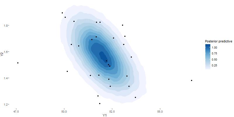
(a) Setting T1.

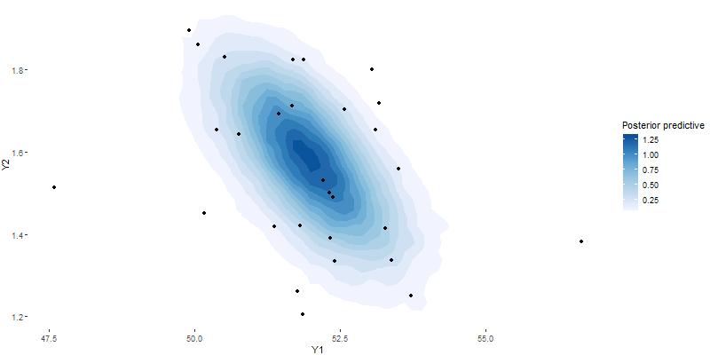
(b) Setting L1.

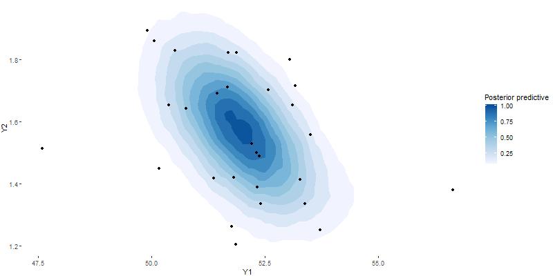
(c) Setting T2.

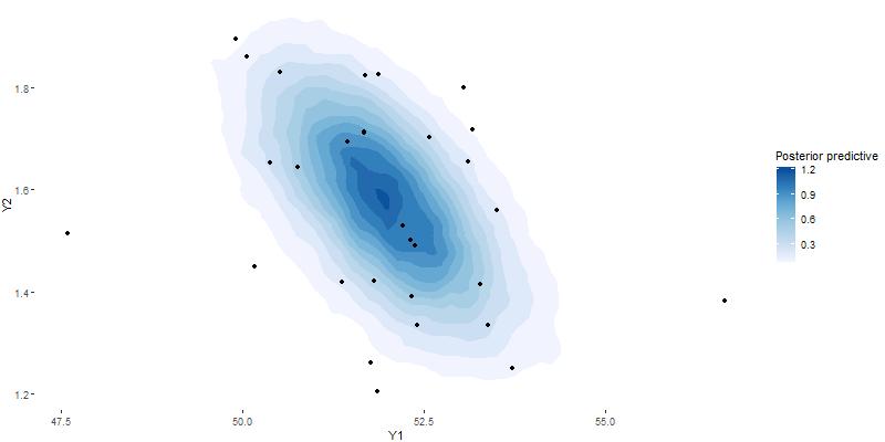
(d) Setting L2.

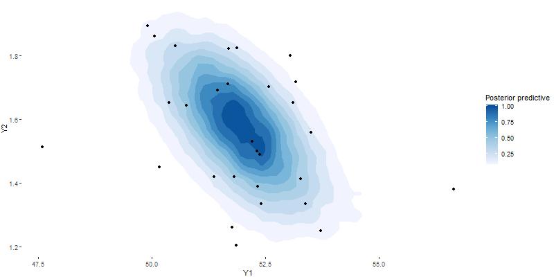
(e) Setting L3.

Figure 5: Examples of the joint posterior predictive distribution of $Y$ obtained under the considered settings. The black dots represents simulated observations $Y$. The left column uses the original model $g$ and the right column uses a linear surrogate.

References

- [1] D. Alvarez-Melis and T.S. Jaakola. On the robustness of interpretability methods. Proceedings of the 2018 ICML Workshop on Human Interpretability in Machine Learning (WHI 2018), Stockholm, Sweden, 2018.
- [2] I. Antoniano-Villalobos, E. Borgonovo, and X. Lu. Nonparametric estimation of probabilistic sensitivity measures. Statistics and Computing, 30:447–467, 2020.
- [3] B. Auder and B. Iooss. Global sensitivity analysis based on entropy. In: Safety, Reliability and Risk Analysis: Theory, Methods and Applications, Martorell et al. (eds), 2009.
- [4] F. Bachoc, G. Blois, J. Garnier, and J.-M. Martinez. Calibration and improved prediction of computer models by universal kriging. Nuclear Science and Engineering, 176:81–97, 2014.
- [5] J.K. Baksalary and F. Pukelshein. Some properties of Matrix Partial Orderings. Linear Algebra and its Applications, 119:57–85, 1989.
- [6] P. Barbillon, C. Barthelémy, and A. Samson. Parameter estimation of complex mixed models based on meta-model approach. Statistics and Computing, 27:1111–1128, 2017.
- [7] P. Barbillon, G. Celeux, A. Grimaud, Y. Lefebvre, and E. Rocquigny (de). Non linear methods for inverse statistical problems. Computational Statistics and Data Analysis, 55:132–142, 2011.
- [8] L.S. Bastos and A. O’Hagan. Diagnostics for Gaussian process emulators. Technometrics, 51(4):425–438, 2009.
- [9] J.O. Berger and L.R. Pericchi. Objective Bayesian Methods for Model Selection: Introduction and Comparison. IMS Lectures Notes – Monograph Series, 2001.
- [10] N. Bochkina. Consistency of the posterior distribution in generalized linear inverse problems. Inverse Problems, 29:095010, 2013.
- [11] E. Borgonovo. A new uncertainty importance measure. Reliability Engineering and System Safety, 92:771–784, 2007.
- [12] N. Bousquet. Diagnostics of prior-data agreement in applied Bayesian analysis. Journal of Applied Statistics, 35:1011–1029, 2008.
- [13] S.P. Brooks and A. Gelman. General methods for monitoring convergence of iterative simulations. Journal of Computational and Graphical Statistics, 7:434–455, 1998.
- [14] B. Broto, F. Bachoc, M. Depecker, and J.-M. Martinez. Sensitivity indices for independent groups of variables. Mathematics and Computers in Simulation, 163:19–31, 2019.
- [15] J. Brynjarsdottir and A. O’Hagan. Learning about physical parameters : The importance of model discrepancy. Inverse Problems, 30:114007, 2014.
- [16] M. Carmassi, P. Barbillon, M. Chiodetti, M. Keller, and E. Parent. Bayesian calibration of a numerical code for prediction. Journal de la Société Française de Statistique, 160:1–30, 2019.
- [17] L. Cavalier. Inverse Problems in Statistics. In P. Alquier, E. Gautier, and G. Stoltz, editors, Inverse Problems and High-Dimensional Estimation, chapter 1, pages 3–96. Springer, 2011.
- [18] G. Celeux, A. Grimaud, Y. Lefebvre, and E. Rocquigny (de). Identifying intrinsic variability in multivariate systems through linearised inverse methods. Inverse Problems in Engineering, 18:401–415, 2010.
- [19] D. Chafaï and J.-M. Loubes. On nonparametric maximum likelihood for a class of stochastic inverse problems. Statistics and Probability Letters, 76:1225–1237, 2006.
- [20] Y. Chen, A. Wiesel, Y.C. Eldar, and A.O. Hero. Shrinkage Algorithms for MMSE Covariance Estimation. IEEE Transactions on Signal Processing, 58:5016–5029, 2010.
- [21] Y. Chung, P.J. Haas, E. Upfal, and T. Kraska. Learning Unknown Examples and Machine Learning Model Generalization. arXiv:808.08294, 2019.
- [22] B.S. Clarke and A.R. Barron. Jeffreys’ prior is asymptotically least favorable under entropy risk. Journal of Statistical Planning and Inference, 41:37–60, 1994.
- [23] C. Cole. Shannon revisited: Information in terms of uncertainty. Journal of the American Society for Information Science, 44:204–211, 1993.
- [24] National Research Council. Assessing the Reliability of Complex Models: Mathematical and statistical foundations of Verification, Validation and Uncertainty Quantification. Washington, DC: The National Academies Press, 2012.
- [25] T.M. Cover and J.A. Thomas. Elements of information theory. John Wiley & Sons, 2012.
- [26] G. Czanner, U.T. Sarma, S.V.and Eden, and E.N. Brown. A signal-to-noise ratio estimator for generalized linear model systems. In Proceedings of the World Congress on Engineering (IIWCE), volume 2, 2008.
- [27] S. Da Veiga. Global sensitivity analysis with dependence measures. Journal of Statistical Computation and Simulation, 85:1283–1305, 2015.
- [28] S. Da Veiga, F. Gamboa, B. Iooss, and C. Prieur. Basics and Trends in Sensitivity Analysis. Theory and Practice in R. SIAM. Computational Science and Engineering, 2021.
- [29] G. Damblin, M. Couplet, and B. Iooss. Numerical studies of space filling designs: optimization of Latin Hypercube Samples and subprojection properties. Journal of Simulation, 7:276–289, 2013.
- [30] G. Damblin, M. Keller, P. Barbillon, A. Pasanisi, and E. Parent. Bayesian model selection for the validation of computer codes. Quality and Reliability Engineering, 32:2043–2054, 2016.
- [31] G. Damblin, M. Keller, P. Barbillon, A. Pasanisi, and E. Parent. Adaptive numerical designs for the calibration of computer codes. SIAM/ASA Journal on Uncertainty Quantification, 6:151–179, 2018.
- [32] M. Dashti, K.J.H. Law, A.M. Stuart, and J. Voss. MAP estimators and their consistency in Bayesian nonparametric inverse problems. Inverse Problems, 29:095017, 2013.
- [33] M. Dashti and A.M. Stuart. The Bayesian Approach to Inverse Problems. In: Ghanem, R. and Higdon, D. and Owhadi, H. (eds). Handbook of Uncertainty Quantification, pages 311–428, 2017.
- [34] A. Deleforge, F. Forbes, and R. Horaud. High-dimensional regression with Gaussian mixtures and partially-latent response variables. Statistics and Computing, 25:893–911, 2015.
- [35] B. Delyon, M. Lavielle, and E. Moulines. Convergence of a stochastic version of the EM algorithm. The Annals of Statistics, 27:94–128, 1999.
- [36] S.E. Dosso. Parallel tempering for strongly nonlinear geoacoustic inversion. The Journal of Acoustical Society of America, 132:3030–3040, 2012.
- [37] S.N. Evans and P.B. Stark. Inverse problems as statistics. Inverse Problems, 18:55–97, 2002.
- [38] P. Farindon. Inequalities in the Löwner Partial Order. In Matrix Inequalities, volume 1790. Lecture Notes in Mathematics.Springer, Berlin, Heidelberg, 2002.
- [39] S. Fu, G. Celeux, N. Bousquet, and M. Couplet. Bayesian inference for inverse problems occurring in uncertainty analysis. International Journal for Uncertainty Quantification, 5:73–98, 2015.
- [40] S. Fu, M. Couplet, and N. Bousquet. An adaptive kriging method for solving nonlinear inverse statistical problems. Environmetrics, 28:e2439, 2017.
- [41] F. Gamboa, A. Janon, T. Klein, and A. Lagnoux. Sensitivity indices for multivariate outputs. Comptes Rendus de l’Académie des Sciences - Paris, 351:307–310, 2013.
- [42] F. Gamboa, A. Janon, T. Klein, and A. Lagnoux. Sensitivity analysis for multidimensional and functional outputs. Electronic Journal of Statistics, 8(1):575–603, 2014.
- [43] D. Garreau and U. von Luxburg. Explaining the Explainer: A First Theoretical Analysis of LIME. Proceedings of the 23rd International Conference on Artificial Intelligence and Statistics (AISTATS) 2020, 108, 2020.
- [44] R. Ghanem, D. Higdon, and H. Owhadi. Introduction to uncertainty quantification. In: Ghanem, R. and Higdon, D. and Owhadi, H. (eds). Handbook of Uncertainty Quantification, pages 3–6, 2017.
- [45] R. Giryes, Y.C. Eldar, A.M. Bronstein, and G. Sapiro. Tradeoffs between convergence speed and reconstruction accuracy in inverse problems. IEEE Transactions on Signal Processing, 66:1676–1690, 2018.
- [46] I Golubic and J. Marovt. On Some Applications of Matrix Partial Orders in Statistics. International Journal of Management, Knowledge and Learning, 9:223–235, 2020.
- [47] J. Hájek. Local Asymptotic Minimax and Admissibility in Estimation. In: Le Cam, L.M. and Neyman, J. and Scott, E.L. (eds). Proceedings of the Sixth Berkeley Symposium on Mathematical Statistics and Probability, 1:175–194, 1972.
- [48] P. Hall and N. Gill. An Introduction to Machine Learning Interpretability. O’Reilly Media, Inc., 2018.
- [49] J. Hauke and A. Markiewicz. On orderings induced by the Loewner partial ordering. Applicationes Mathematicae, 22:145–154, 1994.
- [50] D. Higdon, J. Gattiker, B. Williams, and M. Rightley. Computer model calibration using high-dimensional output. Journal of the American Statistical Association, 103(482):570–583, 2008.
- [51] D. Higdon, M. Kennedy, J. Cavendish, J. Cafeo, and R. Ryne. Combining field data and computer simulations for calibration and prediction. SIAM Journal on Scientific Computing, 26:448–466, 2004.
- [52] B. Iooss, L. Boussouf, V. Feuillard, and A. Marrel. Numerical studies of the metamodel fitting and validation processes. International Journal of Advances in Systems and Measurements, 3:11–21, 2010.
- [53] J. Jacques, C. Lavergne, and N. Devictor. Sensitivity analysis in presence of model uncertainty and correlated inputs. Reliability Engineering and System Safety, 91:1126–1134, 2006.
- [54] J.P. Kaipio and C. Fox. The Bayesian framework for inverse problems in heat transfer. Heat Transfer Engineering, 32:718–753, 2011.
- [55] R.E. Kass and L. Wasserman. The selection of prior distributions by formal rules. Journal of the American Statistical Association, 91:1343–1370, 1996.
- [56] S.M. Kay. Fundamentals of Statistical Signal Processing, Volume I: Estimation Theory. Prenctice Hall, 1993.
- [57] M. Kennedy and A. O’Hagan. Bayesian calibration of computer models (with discussion). Journal of the Royal Statistical Society, 63:425–464, 2001.
- [58] A. Knutson and T. Tao. The honeycomb model of tensor products I: Proof of the saturation conjecture. Journal of the American Mathematical Society, 12:1055–1090, 1999.
- [59] A. Knutson and T. Tao. Honeycomb and sums of Hermitian matrices. Notice of the American Mathematical Society, 48:175–186, 2001.
- [60] J. Koehler and A. Owen. Computer experiments. In: Ghosh, S. and Rao, C. (eds). Design and analysis of experiments, volume 13 of Handbook of Statistics. Elsevier, 1996.
- [61] B. Krzykacz-Hausmann. Epistemic sensitivity analysis based on the concept of entropy. Proceedings of the SAM0’2001 Conference, 2001.
- [62] Gerhard Kurz, Florian Pfaff, and Uwe D. Hanebeck. Kullback-leibler divergence and moment matching for hyperspherical probability distributions. In 2016 19th International Conference on Information Fusion (FUSION), pages 2087–2094, 2016.
- [63] K. Latuszyński, G.O. Roberts, and J.S. Rosenthal. Adaptive Gibbs samplers and related MCMC methods. Annals of Applied Probability, 23:66–98, 2013.
- [64] N. Lawrence. Probabilistic non-linear principal component analysis with Gaussian process latent variable models. Journal of Machine Learning Research, 6:1783–1816, 2005.
- [65] O.P. Le Maître and O.M. Knio. Spectral Methods for Uncertainty Quantification with Applications to Computational Fluid Dynamics. Springer, 2010.
- [66] O. Ledoit and M. Wolf. A Well-Conditioned Estimator for Large-Dimensional Covariance Matrices. Journal of Multivariate Analysis, 88:365–411, 2004.
- [67] G. Lee, W. Kim, H. Oh, B.D. Youn, and N.H. Kim. Review of the statistical model calibration and validation – from the perspectives of uncertainty structures. Structural and Multidisciplinary Optimization, 69:1619–1644, 2019.
- [68] Y. Li and Y. Liang. Learning Mixtures of Linear Regressions with Nearly Optimal Complexity. Proceedings of Machine Learning Research, 75:1–20, 2018.
- [69] Z. Li and D. Hoiem. Learning without Forgetting. IEEE Transactions on Pattern Analysis and Machine Intelligence, 40:2935–2947, 2018.
- [70] E.P. Liski. On Löwner-ordering antitonicity of matrix inversion. Acta Mathematicae Applicatae Sinica, 12:435–442, 1996.
- [71] J. Liu and J. Zhang. New trace bounds for the product of two matrices and their applications in the algebraic Riccati equation. Journal of Inequalities and Applications, 620758, 2009.
- [72] Jun S. Liu. Siegel’s formula via stein’s identities. Statistics and Probability Letters, 21(3):247–251, 1994.
- [73] W. Liu, H. and. Chen and A. Sudjianto. Relative entropy based method for probabilistic sensitivity analysis in engineering design. ASME Journal of Mechanical Design, 128:326–336, 2006.
- [74] A. Ly, M. Marsman, J. Verhagen, R.P.P. Grasman, and E.-J. Wagenmakers. A Tutorial on Fisher information. Journal of Mathematical Psychology, 80:40–55, 2017.
- [75] J.R. Magnus. On differentiating eigenvalues and eigenvectors. Econometric Theory, 1:179–191, 1985.
- [76] T.A. Mara and S. Tarantola. Variance-based sensitivity indices for models with dependent inputs. Reliability Engineering and System Safety, 107:115–121, 2012.
- [77] A.W. Marshall, I. Olkin, and B.C. Arnold. Inequalities: Theory of Majorization and Its Applications. Springer, 2011.
- [78] Tom Minka. Divergence measures and message passing. Technical Report MSR-TR-2005-173, Microsoft Research, January 2005.
- [79] T.P. Minka. Expectation Propagation for Approximate Bayesian Inference. In Proceedings of the Seventeenth Conference on Uncertainty in Artificial Intelligence, pages 362–369, 2001.
- [80] L. Mulugeta, A. Drach, A. Erdermic, C.A. Hunt, M. Horner, J.P. Ku, J.G. Myers Jr., R. Vadigepalli, and W.W. Lytton. Credibility, replicability and reproducibility in simulation for biomedicine and clinical applications in neuroscience. Frontiers in Neuroinformatics, 12:18, 2018.
- [81] J.B. Nagel and B. Sudret. Hamiltonian Monte Carlo and Borrowing Strength in Hierarchical Inverse Problems. ASCE-ASME Journal of Risk and Uncertainty in Engineering Systems, Part A: Civil Engineering, 2, 2016.
- [82] C. Nemeth and P. Fearnhead. Stochastic gradient Markov chain Monte Carlo. Journal of the American Statistical Association, 116:433–450, 2021.
- [83] W.J. Oberkampf and C.J. Roy. Measures of agreement between computation and experiment: validation metrics. Journal of Computational Physics, 217:5–36, 2006.
- [84] W.L. Oberkampf and C.J. Roy. Verification and Validation in Scientific Computing. Cambridge University Press, 2010.
- [85] J.T. Oden and S. Prudhomme. Estimation of modeling error in computational mechanics. Journal of Computational Physics, 182:496–515, 2002.
- [86] A.B. Owen. Sobol’ Indices and Shapley Value. SIAM/ASA Journal on Uncertainty Quantification, 2:245–251, 2014.
- [87] A. Peralta-Alva and M. Santos. Analysis of numerical errors. Working Paper 2012-062A, Research Division, FRB of St. Louis, 2012.
- [88] M. Pereyra, P. Schniter, E. Chouzenoux, J.-C. Pesquet, J.-Y. Tourneret, A.O. Hero, and S. McLaughlin. A survey of stochastic simulation and optimization methods in signal processing. IEEE Journal on Selected Topics in Signal Processing, 10:224–241, 2015.
- [89] E. Perthame, F. Forbes, and A. Deleforge. Inverse regression approach to robust nonlinear high-to-low dimensional mapping. Journal of Multivariate Analysis, 163:1–14, 2018.
- [90] E. Resmerita, H.W. Engl, and A.N. Iusem. The expectation-maximization algorithm for ill-posed integral equations: a convergence analysis. Inverse Problems, 23:2575–2588, 2007.
- [91] A. Saltelli, M. Ratto, T. Andres, F. Campolongo, J. Cariboni, D. Gatelli, M. Saisana, and S. Tarantola. Global sensitivity analysis: the primer. Wiley Online Library, 2008.
- [92] I.M. Sobol. Sensitivity estimates for nonlinear mathematical models. Mathematical Modeling and Computational Experiment. Model, Algorithm, Code, 1(4):407–414 (1995), 1993.
- [93] I.M. Sobol. Global sensitivity indices for nonlinear mathematical models and their Monte Carlo estimates. Mathematics and Computers in Simulation, 55(1-3):271–280, 2001.
- [94] C. Soize. Stochastic Models of Uncertainties in Computational Mechanics. Journal of Sound and Vibration, 332:2739–2395, 2013.
- [95] A.J. Stam. Some inequalities satisfied by the quantities of information of Fisher and Shannon. Information and Control, 2:101–112, 1959.
- [96] P. Stephanov and G. Uhlmann. Linearizing non-linear inverse problems and an application to inverse backscattering. Journal of Functional Analysis, 256:2842–2866, 2009.
- [97] T. Tao. Matrix identities as derivatives of determinant identities. https://terrytao.wordpress.com/2013/01/13/, 2013. Online; accessed 03 February 2020.
- [98] L.O. Tedeschi. Assessment of the adequacy of mathematical models. Agricultural Systems, 89:225–247, 2006.
- [99] L. Tierney. Markov Chain Monte Carlo in Practice. Chapman and Hall, 1995.
- [100] S.J. Vollmer. Posterior consistency for Bayesian inverse problems through stability and regression results. Inverse Problems, 29:125011, 2013.
- [101] J. Von Neumann. Some matrix-inequalities and metrization of matrix-space. Tomsk Univ. Rev., 1:286–300, 1937.
- [102] F. Xie and Y. Xu. Bayesian Projected Calibration of Computer Models. Journal of the American Statistical Association, in press, 2020.
- [103] R. Yang and J.O. Berger. A catalog of noninformative priors. Technical Report, Duke University, 1998.
- [104] S. Yang, F. Xiong, and F. Wang. Polynomial Chaos Expansion for Probabilistic Uncertainty propagation. In: Hessling, J.P. (eds). Uncertainty Quantification and Model Calibration. IntechOpen, 2017.