Systematic investigation of the Hoyle-analog states in light nuclei.

Abstract

We investigate resonance states in three-cluster continuum of some light nuclei ⁹Be, ⁹B, ¹⁰B, ¹¹B and ¹¹C. These nuclei are considered to have a three-cluster configuration consisting of two alpha-particles and neutron, proton, deuteron, triton and nucleus ³He. In this study, we make use two different microscopic three-cluster models. The first model employs the Hyperspherical Harmonics basis to numerate channels and describe three-cluster continuum. The second model is the well-known complex scaling method. The nucleon-nucleon interaction is modeled by the semi-realistic Minnesota and Hasegawa-Nagata potentials. Our main aim is to find the Hoyle-analog states in these nuclei or, in other words, whether it is possible to synthesize these nuclei in a triple collision of clusters. We formulate the criteria for selecting such states and apply them to resonance states, emerged from our calculations. We found that there are resonance states obeying the formulated criteria which make possible syntheses of these nuclei in a stellar environment.

I Introduction

We are going to search and analyze properties of the Hoyle-like states in light nuclei. It is necessary to recall that the Hoyle state is a very narrow resonance state in ¹²C, which was predicted by Fred Hoyle in 1954 Hoyle (1954). Three years later this state was experimentally observed by studying beta decays of ¹²B in Ref. Cook et al. (1957). It is interesting to point out that F. Hoyle predicted the energy of the $0^{+}$ resonance state at $E$ =0.33 MeV above the three alpha-particles threshold, and Cook et al in Ref. Cook et al. (1957) determined the position of the resonance state at $E$= 0.372$\pm$0.002MeV. One has to compare to the modern value of the energy which is $E$=0.3796$\pm$0.0002 MeV J. H. Kelley and J. E. Purcell and C. G. Sheu (2017). This resonance state created by a triple collision of three alpha-particles is the key element in syntheses of atomic nuclei starting from ¹²C. The Hoyle state is a way for the nucleosynthesis of carbon in helium-burning red giant stars, which are rich of alpha-particles. Actually, F. Hoyle was the first who proclaimed that nuclear synthesis can take place in a triple collision of light nuclei, namely alpha-particles. Such processes are very difficult to be organized in laboratory, but the Nature has time and facilities to carry out such processes in the inside of stars. One can find more interesting historical facts and scientific results about the Hoyle state in the review Freer and Fynbo (2014).

Two important quotations from F. Hoyle paper Hoyle (1954):

1. ”It was pointed out some years ago by H. Bethe Bethe (1939) that effective element-building inside starts must proceed, in the absence of hydrogen, by triple collisions as a starting point:

   $$3\alpha\rightarrow^{12}\text{C}+\gamma."$$ (1)

2. ”It is convenient to replace reaction (1) by

   $$\alpha+\alpha\rightarrow^{8}Be,\quad^{8}Be+\alpha\rightarrow^{12}C+\gamma.$$ (2)

   This is a permissible step, since the lifetime of the unstable ⁸Be is appreciably longer than the time required for nuclear collision of two $\alpha$ particles; that is, longer than the $\alpha$ particle radius divided by the relative velocity”.

These two equations (1) and (2) represent two different ways of excitation of the Hoyle resonance state and two different ways of syntheses of ¹²C. However, in both scenarios the very narrow $0^{+}$ resonance state is the key factor in creation of the carbon 12.

There are a very large number of publications devoted to the $0^{+}$ and other resonance states in ¹²C. Different methods have been used to determine parameters of the Hoyle state and to shed some light on the nature of this states and other resonances states, residing in the three-cluster continuum in ¹²C. However, only few publications (Kanada-En’yo (2007); Yamada and Funaki (2010); Kanada-En’yo et al. (2011); Suhara and Kanada-En’yo (2012); Yamada and Funaki (2012); Kanada-En’yo and Suhara (2015); Zhou and Kimura (2017); Chiba and Kimura (2018)) have been aimed at finding the Hoyle-analog states in light nuclei. They are mainly concentrated on closest neighbors of the ¹²C nucleus, namely, ¹¹B, ¹¹C and ¹³C. In Refs. Yamada and Funaki (2010) and Yamada and Funaki (2012) the structure of 1/2⁺ and 3/2^- states in ¹¹B has been investigated within the three-cluster orthogonality condition model (OCM) combined with the Gauss expansion method. In these papers, parameters of resonance states were obtained by using the complex scaling technique. By analyzing properties of wave functions, the authors of the Refs. Yamada and Funaki (2010, 2012) came to the conclusion that the 1/2⁺ resonance state the parameters $E$ = 0.75 MeV and $\Gamma$= 190 keV can be considered as the Hoyle-analog states. The antisymmetrized molecular dynamics (AMD) has been used to study the excited states of the negative parity in ¹¹B and ¹¹C in Refs. Kanada-En’yo (2007); Kanada-En’yo et al. (2011). It was concluded that the third excited states in ¹¹B and ¹¹C have a dilute cluster structure $\alpha+\alpha+t$ and $\alpha+\alpha+^{3}$He, respectively, and can be treated as the Hoyle analog states.

In the present paper we consider these nuclei and also ⁹Be, ⁹B and ¹⁰B. We also consider a large number of states with different values of the total momentum $J$ and both of negative and positive parities. Before starting in searching for the Hoyle-analog states, one needs to formulate clear criteria for selecting such states. By analyzing properties of the Hoyle state, one may suggest the following criteria for the Hoyle analog states in three-cluster systems:

1. Very narrow resonance state,

2. Resonance state which lies close to three-cluster threshold,

3. Resonance state which has the total orbital momentum $L=0$.

We consider the first criterion as the most important as in the case of very narrow (long-lived) resonance states, and a compound system has more chances to be reconstructed and transformed in to a bound state. However, we will analyze all resonance states.

Our main aim is to find the Hoyle-analogue states in light nuclei ⁹Be and ⁹B, ¹⁰B, ¹¹B and ¹¹C. In other words, we are going to study whether light nuclei can be created in triple collision of clusters. The necessary condition for such a process is the existence of a very narrow resonance state in three-cluster continuum. Actually we consider a chain of reactions

$$A_{1}+A_{2}+A_{3}=A^{\ast}\Rightarrow A+\gamma$$

which consists of two steps. In the first step, an excited state (very narrow resonance state) of a compound nucleus is created in a triple collision of clusters consisting of $A_{1}$, $A_{2}$ and $A_{3}$ nucleons. In the second step, the compound nucleus by emitting a photon transits from the resonance state to the bound state. The narrower is a resonance state in the first step, the more is the probability to transit from the resonance to the bound state. For each nuclei we determine energy and width of resonance states. We select a resonance state with a very small width. We also analyze the wave function of selected resonance states. These investigations will be performed within a microscopic three-cluster model which involves the hyperspherical harmonics to distinguish channels of the three-cluster system. For this model, which was formulated in Ref. Vasilevsky et al. (2001a), we use the abbreviation AMHHB which means the algebraic model of scattering making use of the hyperspherical harmonics basis. In Ref. Vasilevsky et al. (2012) this model has been applied to study bound and resonance states in ¹²C. It fairly good reproduced the energy and width of the Hoyle state in ¹²C. And it was demonstrated that this model is in good agreement with other alternative models, for instance, the complex scaling method. Note that the most effective methods among others, which are used to study resonance states in three-cluster and many-channel systems, are the Complex Scaling Method and Hyperspherical Harmonics Method

We present results obtained with both methods. The AMHHB method, which employs hyperspherical harmonics to numerate channels of three-cluster continuum, allows us to determine energy and width of a resonance state, reveals the dominant decay channels, and sheds more light on the nature of the resonance state by analyzing its wave functions. This model correctly treats the Pauli principle and makes uses of the semi-realistic nucleon-nucleon potential. The complex scaling method (CSM), which also uses this type of the nucleon-nucleon interaction, is more advance and model independent method to determine the poles of the $S$-matrix in two- and three-cluster systems. Note that both methods give very close results for narrow resonance states and different resonance parameters for wide resonance states.

The preliminary analysis of three-cluster resonance states in ⁹B and ⁹B has been carried out in Ref. Vasilevsky et al. (2017), and resonance states have been investigated in the mirror nuclei ¹¹B and ¹¹C in Ref. Vasilevsky (2013). In Ref. Nesterov et al. (2014a) the AMHHB model was applied to study the spectrum of bound states in ¹⁰B. To make a systematic analysis of resonance states and to discover the Hoyle analog state in ⁹Be, ⁹B, ¹⁰B, ¹¹B and ¹¹C we have to make additional calculations and thorough investigations of  peculiarities of resonance wave functions.

The present paper is organized in the following way. In Sec. II we shortly explain the main idea of the microscopic method which involves the hyperspherical harmonics for description of bound and scattering states of a three-cluster system. Results of numerical calculations and discussions of the results obtained are presented in Sec. III. We start with the reexamination of properties of the Hoyle state. We also consider other resonance states in ¹²C to display similarities and differences between them. This is done within the AMHHB and CSM in order to formulate more clear criteria for selecting the Hoyle-analog states. And then we proceed with analysis of resonance states in three-cluster continuum of nuclei ⁹Be, ⁹B, ¹⁰B, ¹¹B and ¹¹C. By applying the formulated criteria, we select the Hoyle-analog states and describe their properties. Sect. IV present a summary of our investigations.

II Method

II.1 Three-cluster wave function

To study three-cluster systems we exploit a microscopic model which incorporates the Resonating Group Method, the $J$-matrix Method or the algebraic version of the Resonating Group Method (RGM) and the Hyperspherical Harmonics Method. Details of the model and its application to study of bound and continuous spectrum states of light nuclei can be found in Refs. Vasilevsky et al. (2001a, b); Broeckhove et al. (2007); Nesterov et al. (2010); Vasilevsky et al. (2012); Vasilevsky (2013) and Nesterov et al. (2014b).

The standard ansatz of the RGM for representing the wave function of a three–$s$-cluster system is used

$$\Psi_{E,J} = \sum_{S,L}\widehat{\mathcal{A}}\left\{\left[\Phi_{1}\left(A_{1}\right)\Phi_{2}\left(A_{2}\right)\Phi_{3}\left(A_{3}\right)\right]_{S}\right.$$

$$\times \left.\psi_{E,LJ}\left(\mathbf{x},\mathbf{y}\right)\right\}_{J},$$

where the wave function $\psi_{E,LJ}\left(\mathbf{x},\mathbf{y}\right)$ describes relative motion of clusters  and the antisymmetric functions $\Phi_{\nu}\left(A_{\nu}\right)$ ($\nu$=1, 2, 3) describes internal motion of nucleons inside the cluster with index $\nu$. Two vectors $\mathbf{x}$ and $\mathbf{y}$ denote one of the possible sets of the Jacobi vectors. Within this paper, the vector $\mathbf{x}$ determines distance between two selected clusters, while the vector $\mathbf{y}$ represents displacement of the third cluster with respect to the center of mass of two selected clusters. The antisymmetrization operator $\widehat{\mathcal{A}}$ provides  full antisymmetrization of the wave function of a compound system. By assuming $\widehat{\mathcal{A}}=1$ and the orthogonality condition to the Paul-forbidden states, one transits to the OCM.

It is very convenient to use the $LS$ coupling scheme for three interacting $s$-clusters. In this scheme, the total spin $S$ is a vector sum of individual spins of clusters, and the total orbital momentum $L$ is also a vector sum of the partial orbital momenta $\widehat{\mathbf{l}}_{x}$ and $\widehat{\mathbf{l}}_{y}$, associated with the Jacobi vectors $\mathbf{x}$ and $\mathbf{y}$, respectively. The total angular momentum $J$ is a vector sum of the total orbital momentum $L$ and the total spin $S$.

To simplify of obtaining wave functions of discrete and continuous spectrum states and scattering parameters, we transit from the Jacobi vectors $\mathbf{x}$ and $\mathbf{y}$ to the hyperspherical coordinates which consist of hyperradius $\rho$ and five hyperspherical angles which we denote as $\Omega_{5}$. The hyperradius $\rho$ is defined in unambiguous way

$$\rho=\sqrt{\mathbf{x}^{2}+\mathbf{y}^{2}},$$ (4)

while there are several different ways for definition of the hyperspherical angles (see for instance, Zickendraht (1965); A. Avery (1989); R. I. Dzhibuti, N. B. Krupennikova (1984)). We make use the most popular set of hyperspherical angles which was suggested by Zernike and Brinkman in 1935 Zernike and Brinkman (1935). This set consists of the hyperspherical angle $\theta$ which determines relative lengths of the Jacobi vectors

$$x=\rho\cos\theta,\quad y=\rho\sin\theta,$$ (5)

two angles $\theta_{x}$and $\phi_{x}$, determining orientation of vector $\mathbf{x}$, and two other angles $\theta_{y}$ and $\phi_{y}$, determining orientation of vector $\mathbf{y}$ in the space. Note, that the angles $\left\{\theta_{x},\phi_{x}\right\}$ describe rotation of a two-cluster subsystem and the angles $\left\{\theta_{y},\phi_{y}\right\}$ describe rotation of the third cluster around center of mass of the two-cluster subsystem. Five hyperspherical angles are able to describe any shape and any orientation (i.e. rotation) of a triangle connecting centers of mass of three clusters, and hyperradius determines any size of that triangle.

Having introduced the hyperspherical coordinate, we can represent the three-cluster wave function (II.1) in the following form

$$\Psi_{E,J} =\sum_{c}\widehat{\mathcal{A}}\left\{\left[\Phi_{1}\left(A_{1}\right)\Phi_{2}\left(A_{2}\right)\Phi_{3}\left(A_{3}\right)\right]_{S}\right.$$ (6)

$$\times\left.\psi_{E,c}\left(\rho\right)\mathcal{Y}_{c}\left(\Omega_{5}\right)\right\}_{J},$$

where $c$ is a multiple index $c=\left\{K;\lambda,l;L,S\right\}$ classifying channels of the three-cluster system and involving the hypermomentum $K$, partial orbital momenta $\lambda$ and $l$ associated with the Jacobi vectors $\mathbf{x}$ and $\mathbf{y}$, respectively, and the total orbital momentum $L$. The hyperspherical harmonics $\mathcal{Y}_{c}\left(\Omega_{5}\right)$ form a complete set of functions on five-dimension sphere and thus account for all kinds of motion of a three-cluster system. Components of the many-channel hyperradial wave function $\left\{\psi_{E,c}\left(\rho\right)\right\}$ have to be determined by solving the Schrödinger equation with the selected nucleon-nucleon potential.

II.2 Three-cluster equation

For three structureless particles one obtains the infinite set of differential equations

$$\sum_{\widetilde{c}}\left[\delta_{c,\widetilde{c}}\widehat{T}_{K}+V_{c,\widetilde{c}}\left(\rho\right)\right]\psi_{E,\widetilde{c}}\left(\rho\right)=E\psi_{E,c}\left(\rho\right),$$ (7)

where

$$\widehat{T}_{K}=-\frac{\hbar^{2}}{2m}\left[\frac{\partial^{2}}{\partial\rho^{2}}+\frac{5}{\rho}\frac{\partial}{\partial\rho}-\frac{K\left(K+4\right)}{\rho^{2}}\right].$$ (8)

Matrix $\left\|V_{c,\widetilde{c}}\left(\rho\right)\right\|$ of the effective potential energy is determined as matrix elements of interaction $\widehat{V}$ between the hyperspherical harmonics

$$V_{c,\widetilde{c}}\left(\rho\right)=\left\langle\mathcal{Y}_{c}\left|\widehat{V}\right|\mathcal{Y}_{\widetilde{c}}\right\rangle,$$ (9)

where integration is performed over all hyperspherical angles $\Omega_{5}$. If particles have electric charges, than we have the following contribution

$$V_{c,\widetilde{c}}^{\left(C\right)}\left(\rho\right)=\frac{Z_{c,\widetilde{c}}e^{2}}{\rho}$$ (10)

from the Coulomb interaction to the potential energy $V_{c,\widetilde{c}}\left(\rho\right)$ (9). The quantity $Z_{c,\widetilde{c}}$ can be called the effective charge. Assuming that at a large values of hyperradius the effective potential $V_{c,\widetilde{c}}\left(\rho\right)$ originated from a short range particle-particle interaction is negligibly small, and omitting non-diagonal elements of the effective charge (that is putting $Z_{c,\widetilde{c}}=0$ for $c\neq\widetilde{c}$), we obtain an asymptotic part of the channel Hamiltonian

$$\widehat{H}_{c}^{\left(A\right)}=\left\{-\frac{\hbar^{2}}{2m}\left[\frac{\partial^{2}}{\partial\rho^{2}}+\frac{5}{\rho}\frac{\partial}{\partial\rho}-\frac{K\left(K+4\right)}{\rho^{2}}\right]+\frac{Z_{c,c}e^{2}}{\rho}\right\}.$$ (11)

Eigenfunctions of this Hamiltonian describing incoming and outgoing hyperradial waves can be easily found and expressed through the Whittaker functions (see chapter 13.1 in Ref. Abramowitz and Stegun (1972))

$$\psi_{c}^{\left(\pm\right)}\left(\rho,\eta_{c}\right)=\sqrt{\frac{\pi}{2}}\frac{1}{\rho^{5/2}}W_{\mp i\eta_{c},K+2}\left(\mp 2ik\rho\right),$$ (12)

where

$$k=\sqrt{\frac{2mE}{\hbar^{2}}}$$

and $\eta_{c}$ is the Sommerfeld parameter for the three-cluster system

$$\eta_{c}=\frac{m}{\hbar^{2}}\frac{Z_{c,c}e^{2}}{k}.$$

Thus, the boundary conditions or the asymptotic form of many-channel wave functions can be expressed in the form

$$\psi_{E,c}\left(\rho\right)=\delta_{c_{0},c}\psi_{c}^{\left(-\right)}\left(\rho,\eta_{c}\right)-S_{c_{0},c}\psi_{c}^{\left(+\right)}\left(\rho,\eta_{c}\right),$$

where $c_{0}$ stands for an incoming channel, $S_{c_{0},c}$ is an element of the scattering $S$-matrix.

For three-cluster systems, when the internal structure of clusters and the Pauli principle are taking into account, we obtain the set of integro-differential equations:

$$\sum_{\widetilde{c}}\left[\delta_{c,\widetilde{c}}\widehat{T}_{K}\psi_{E,\widetilde{c}}\left(\rho\right)+\int d\widetilde{\rho}\widetilde{\rho}^{5}V_{c,\widetilde{c}}\left(\rho,\widetilde{\rho}\right)\psi_{E,\widetilde{c}}\left(\widetilde{\rho}\right)\right]$$ (13)

$$=E\sum_{\widetilde{c}}\int d\widetilde{\rho}\widetilde{\rho}^{5}N_{c,\widetilde{c}}\left(\rho,\widetilde{\rho}\right)\psi_{E,\widetilde{c}}\left(\widetilde{\rho}\right).$$

This system of equations can be obtained from the many-particle Schrödinger equations with the help of the projection operator

$$\widehat{P}_{c}\left(\rho\right)=\widehat{\mathcal{A}}\left\{\left[\Phi_{1}\left(A_{1}\right)\Phi_{2}\left(A_{2}\right)\Phi_{3}\left(A_{3}\right)\right]_{S}\delta\left(\rho-\overline{\rho}\right)\mathcal{Y}_{c}\left(\Omega_{5}\right).\right\}$$ (14)

Applying this operator to the unit operator, we obtain the norm kernel $N_{c,\widetilde{c}}\left(\rho,\widetilde{\rho}\right)$

$$N_{c,\widetilde{c}}\left(\rho,\widetilde{\rho}\right)=\left\langle\widehat{P}_{c}\left(\rho\right)|\widehat{P}_{\widetilde{c}}\left(\widetilde{\rho}\right)\right\rangle.$$ (15)

In this expression integration is performed over all spacial coordinates (the Jacobi vectors) and over all spin and isospin coordinates as well. The matrix of the potential energy is related to matrix elements of the microscopic Hamiltonian $\widehat{H}$ by the relation

$$V_{c,\widetilde{c}}\left(\rho,\widetilde{\rho}\right)=\left\langle\widehat{P}_{c}\left(\rho\right)\left|\widehat{H}\right|\widehat{P}_{\widetilde{c}}\left(\widetilde{\rho}\right)\right\rangle-\delta_{c,\widetilde{c}}\widehat{T}_{K}\delta\left(\rho-\widetilde{\rho}\right).$$ (16)

The system of Eq. (13) can be directly solved by reducing to the reasonable finite number of involved three-cluster channels $N_{c}$ and with the boundary conditions determined above. Solutions of the systems yields us the definite set of matrix elements of the $S$ matrix. They describe all kinds of elastic and inelastic processes in a three-cluster system.

Note that the operator (14) is a straightforward generation of the projection operator which has been used for two-cluster systems (see Ref. Tang et al. (1978)). In three-cluster systems, we can easily perform this operation though we do not explain the details here.

Within the present model a wave function (II.1) of a three-cluster system is expanded over an infinite set of cluster oscillator functions $\left|n_{\rho},c\right\rangle$

$$\Psi_{E,LJ}=\sum_{n_{\rho},c}C_{n_{\rho},c}^{E,J}\left|n_{\rho},c\right\rangle,$$

where

$$\left|n_{\rho},c\right\rangle=\left|n_{\rho},K;\lambda,l;L\right\rangle$$

$$= \widehat{\mathcal{A}}\left\{\Phi_{1}\left(A_{1}\right)\Phi_{2}\left(A_{2}\right)\Phi_{3}\left(A_{3}\right)R_{n_{\rho}K}\left(\rho,b\right)\mathcal{Y}_{c}\left(\Omega_{5}\right)\right\},$$

$\mathcal{Y}_{c}\left(\Omega_{5}\right)$ is a hyperspherical harmonic with the quantum numbers $c=\left\{K,l_{x},l_{y},L\right\}$ and $R_{n_{\rho},K}\left(\rho,b\right)$ is an oscillator function

$$R_{n_{\rho},K}\left(\rho,b\right) = \left(-1\right)^{n_{\rho}}\mathcal{N}_{n_{\rho},K}$$

$$\times r^{K}\exp\left\{-\frac{1}{2}r^{2}\right\}L_{n_{\rho}}^{K+3}\left(r^{2}\right),$$

$$r = \rho/b,\quad\mathcal{N}_{n_{\rho},K}=b^{-3}\sqrt{\frac{2\Gamma\left(n_{\rho}+1\right)}{\Gamma\left(n_{\rho}+K+3\right)}},$$

and $b$ is an oscillator length.

In this case, a set of the integro-differential equations is reduced to a set of the algebraic (matrix) equations

$$\sum_{\widetilde{n}_{\rho},\widetilde{c}}\left[\left\langle n_{\rho},c\left|\widehat{H}\right|\widetilde{n}_{\rho},\widetilde{c}\right\rangle-E\left\langle n_{\rho},c|\widetilde{n}_{\rho},\widetilde{c}\right\rangle\right]C_{\widetilde{n}_{\rho},\widetilde{c}}^{E,J}=0,$$ (19)

which can be more easily solved by the numerical methods than the set of equations (13). For continuous spectrum states one has to impose proper boundary conditions for expansion coefficients $\left\{C_{n_{\rho},c}^{E,J}\right\}$. These conditions have been discussed in Ref. Vasilevsky et al. (2001a) where relations between the discrete $\left\{C_{n_{\rho},c}^{E,J}\right\}$ and continuous $\left\{\psi_{E,c}\left(\rho\right)\right\}$ wave functions were established. By including the asymptotic form of expansion coefficients $\left\{C_{n_{\rho},c}^{E,J}\right\}$, which is valid for large values of hyperradial excitations $n_{\rho}\gg 1$, we obtain in a closed form the system of equations determining both wave functions of a continuous spectrum and the corresponding $S$ matrix.

II.3 Supplementary quantities

Having obtained the expansion coefficients for any state of the three-cluster continuum, we can easily construct its wave function in the coordinate space. It can be done, the first of all, for the total hyperradial wave function

$$\psi_{E,c}\left(\rho\right)=\sum_{n_{\rho}}C_{n_{\rho},c}^{E,J}R_{n_{\rho},K}\left(\rho,b\right).$$ (20)

It can be also done for the wave function

$$\psi_{E,LJ}\left(\mathbf{x},\mathbf{y}\right)=\sum_{n_{\rho},c}C_{n_{\rho},c}^{E,J}R_{n_{\rho},K}\left(\rho,b\right)\mathcal{Y}_{c}\left(\Omega_{5}\right).$$ (21)

To get more information about the state under consideration we will study different quantities which can be obtained with the wave function in discrete or coordinate spaces. With wave functions in the discrete oscillator quantum number representation we can determine a weight $W_{sh}$ of the oscillator function belonging to the oscillator shell $N_{sh}$ in this wave function:

$$W_{sh}\left(N_{sh}\right)=\sum_{n_{\rho},c\in N_{sh}}\left|C_{n_{\rho},c}^{E,J}\right|^{2}.$$ (22)

where the summation is performed over all hyperspherical harmonics and hyperradial excitations obeying the following condition:

$$N_{os}=2n_{\rho}+K.$$

Here $N_{os}$ is fixed. Basis wave functions (II.2) belongs to the oscillator shell with the number of oscillator quanta $N_{os}=2n_{\rho}+K$. It is convenient to numerate the oscillator shells by $N_{sh}$ ( = 0, 1, 2, . . . ), which we determine as

$$N_{os}=2n_{\rho}+K=2N_{sh}+K_{\min},$$

where $K_{\min}=L$ for normal parity states $\pi=\left(-1\right)^{L}$ and $K_{\min}=L+1$ for abnormal parity states $\pi=\left(-1\right)^{L+1}$. Thus we account oscillator shells starting from a ”vacuum” shell ($N_{sh}$ = 0) with minimal value of the hypermomentum $K_{\min}$ compatible with a given total orbital momentum $L$.

The weights $W_{sh}$ we will calculate both for bound and resonance states. For a bound state, the wave function is normalized by the condition

$$\left\langle\Psi_{E,J}|\Psi_{E,J}\right\rangle=\sum_{n_{\rho},c}\left|C_{n_{\rho},c}^{E,J}\right|^{2}=1,$$ (23)

and this quantity $W_{sh}$ determines the probability. For the continuous spectrum state, when the wave function is normalized by the condition

$$\left\langle\Psi_{E,J}|\Psi_{\widetilde{E},J}\right\rangle=\sum_{n_{\rho},c}C_{n_{\rho},c}^{E,J}C_{n_{\rho},c}^{\widetilde{E},J}=\delta\left(k-\widetilde{k}\right),$$ (24)

this quantity has a different meaning. It determines the relative contribution of the different oscillator shells and also the shape of the resonance wave function in the oscillator representation.

It is worthwhile to notice that oscillator functions have some important features. Oscillator functions belonging to an oscillator shell $N_{sh}$ allow one to describe a many-particle system in a finite range of hyperradius $0<\rho\leq b\sqrt{4N_{sh}+K_{\min}+3}$. Outside this region, these oscillator functions give a negligible small contribution to many-particle wave function. This statement is, for example, demonstrated in Ref. Vasilevsky et al. (2018). Thus, oscillator functions with a small value of $N_{sh}$ describe very compact configurations of a three-cluster system with all clusters being close to each other. When $N_{sh}$ is large, the oscillator functions represent a dispersed (dilute) configurations. There are two principal regimes in these configurations. The first regime is associated with a two-body type of asymptotic when two clusters are at a small distance and the third cluster is moved far away. The second regime accounts for the case when all three clusters are well separated. Taking these into account, we will deduce from an analysis of shell weights $W_{sh}$ whether a wave function of a bound or resonance state describes a compact or dispersed three-cluster configuration.

By employing the wave function in the coordinate space we determine the correlation function

$$D\left(x,y\right)=x^{2}y^{2}\int\left|\psi_{E,LJ}\left(\mathbf{x},\mathbf{y}\right)\right|^{2}d\widehat{\mathbf{x}}d\widehat{\mathbf{y}}$$ (25)

and average distances $R_{1}$ and $R_{2}$ between clusters

$$R_{1} =\sqrt{\frac{A}{\left(A_{1}+A_{2}\right)A_{3}}}\sqrt{\int y^{2}\left|\psi_{E,LJ}\left(\mathbf{x},\mathbf{y}\right)\right|^{2}d\mathbf{x}d\mathbf{y}},$$ (26)

$$R_{2} =\sqrt{\frac{\left(A_{1}+A_{2}\right)}{A_{1}A_{2}}}\sqrt{\int x^{2}\left|\psi_{E,LJ}\left(\mathbf{x},\mathbf{y}\right)\right|^{2}d\mathbf{x}d\mathbf{y}}.$$ (27)

In our notations, $R_{2}$ determines an average distance between alpha-particles, while $R_{1}$ determines a distance of the third cluster to the center of mass of two alpha particles. Note that in Eq. (25) integration is performed over unit vectors $\widehat{\mathbf{x}}\$and $\widehat{\mathbf{y}}$, while in Eqs. (26) and (27) integration is carried out over all Jacobi vectors or all hyperspherical coordinates.

It is obvious, that the correlation function $D\left(x,y\right)$ can be determined both for bound and resonance states. However, the average distances $R_{1}$ and $R_{2}$ can be calculated for the bound state only, since  for resonance states integrals in Eqs. (26) and (27) diverge. In Ref. Vasilevsky et al. (2017) we suggested to extent to resonance states the definition of average distances $R_{1}$ and $R_{2}$.  For this aim we restricted the integration within the internal part of the resonance wave functions which was normalized to unity. Recall that the internal part of a wave function is represented in the region (0$\leq\rho\leq\rho_{\max}$ in the coordinate space or 0$\leq n_{\rho}\leq N^{\left(i\right)}$ in the oscillator space) where distances between clusters are relatively small and effects intercluster interactions are very strong. Such the definition of $R_{1}$ and $R_{2}$ allows us to study the shape of the triangle, composed by three interacting clusters, but not its size. By comparing average distances $R_{1}$ and $R_{2}$ for different resonances of the same or other nucleus, we obtain more information on the structure of the resonance wave functions.

It is important to note, that the oscillator basis (II.2) can be used to determine parameters of resonance states within the methodology of the complex scaling method. It will be demonstrated in other paper. However, it is more expedient to use the Gaussian basis in the six-dimension space to perform such a type of calculations, as this basis provides more rapid convergence of results than the oscillator basis.

III Results and discussions.

For all nuclei under consideration we employ the Minnesota potential (Thompson et al. (1977); Reichstein and Tang (1970))  (MP) or the modified Hasegawa-Nagata potential Hasegawa and Nagata (1971); Tanabe et al. (1975) (MHNP). Both the central and spin-orbital components of these potentials are taken into account.

In such a type of calculations we have only one free parameter to be selected. This is the oscillator length $b$ which is common for all clusters of a compound nucleus and effectively determines the spatial distribution of nucleons in clusters. In our calculations the oscillator length $b$ is fixed by minimizing the energy of the three-cluster threshold. For ⁹Be, ⁹B and ¹²C, the oscillator length $b$ minimizes the energy of an alpha-particle.

The Majorana parameter $m$ of the MHNP and the exchange parameter $u$ of the MP are very often used as an adjustable parameter. If one adjusts these parameters to reproduce phase shifts of the $\alpha-\alpha$ scattering and parameters of resonance states in ⁸Be, one obtains the overbound the $0^{+}$ and $2^{+}$ states in ¹²C, and also the $4^{+}$ bound state which contradicts to the experimental data. This problem was discussed in Ref. Vasilevsky et al. (2012) where the MP was used to calculate spectrum of bound and resonance states in ¹²C. Such a problem also appears for all nuclei under considerations. This problem has been discussed in Refs. Nesterov et al. (2014b); Vasilevsky et al. (2017) where spectra of ⁹B and ⁹Be were investigated. To avoid appearance unphysical bound states, we adjust parameters $m$ and $u$ to reproduce the energy of the ground state measured from the three-cluster threshold. For mirror nuclei ⁹Be and ⁹B, ¹¹B and ¹¹C, we adjust these parameters only for one nucleus of these pairs; for ⁹B and ¹¹B. This is done in order to study effects of the Coulomb interaction on parameters of bound and resonance states. In Table 1 we collected input parameters for each nucleus. We also demonstrate the energy ($E_{R}$) and width ($\Gamma_{R}$) of the 0⁺ resonance state in ⁸Be, obtained with these input parameters.

Table 1: List of nuclei investigated within microscopic three-cluster models and input parameters; $b$ - oscillator length, $m$ or $u$ - exchange parameters of the NN interaction. $E_{R}$ (MeV) and $\Gamma_{R}$ (keV) are parameters of the $0^{+}$ resonance state in ⁸Be.

Nucleus	3CC	Potential	$u$ or $m$	$b$, fm	$E_{R}$	$\Gamma_{R}$,
${}^{9}Be$	$\alpha+\alpha+n$	MHNP	0.0332	1.317	0.859	958.4
${}^{9}B$	$\alpha+\alpha+p$	MHNP	0.0332	1.317	0.859	958.4
${}^{10}B$	$\alpha+\alpha+d$	MP	0.915	1.395	0.426	69.0
${}^{11}B$	$\alpha+\alpha+^{3}H$	MP	0.920	1.322	0.317	19.8
${}^{11}C$	$\alpha+\alpha+^{3}He$	MP	0.920	1.322	0.317	19.8
${}^{12}C$	$\alpha+\alpha+\alpha$	MP	0.940	1.285	0.022	2.33$\cdot 10^{-5}$

One can see that by selecting the optimal values of the parameters $u$ and $m$ of nucleon-nucleon interaction, we make very broad the 0⁺ resonance state in ⁸Be.

Having determined the oscillator length $b$ and the parameter of the nucleon-nucleon forces, we have to select a part of the total Hilbert space which takes part in construction of the wave function of three-cluster continuous states. This part is restricted by the number of the three-cluster channels $c$ and the number of hyperradial excitations or, in other words, the maximal number of oscillator shell. In all our calculations we use a standard set of the hyperspherical harmonics and hyperradial excitations. Positive parity states are calculated with the hyperspherical harmonics $K_{\min}\leq K\leq K_{\max}$. where $K_{\max}=14$ for the positive parity states and $K_{\max}=13$ for the negative parity states. The minimal value of the hypermomentum $K_{\min}$ equals the total orbital momentum $L$ for normal parity states $\pi=\left(-1\right)^{L}$ and $K_{\min}=L+1$ for the non-normal parity states. The total number of channels  $N_{ch}$ depends on the total angular momentum $J$, the possible values of the total orbital moment $L$ and symmetry properties of a three-cluster system. To achieve the asymptotic region and to provide sufficient precision of our calculations we take into account the hyperradial excitation up to 70. This value of hyperradial excitations and the number of the hyperspherical channels cover a large range of intercluster distances and different shapes of the three-cluster triangle.

In this paper we will not discuss the dependence of parameters of resonance states on $K_{\max}$ and $N_{ch}$, and the convergence of the obtained results, as they were addressed in Refs. Nesterov et al. (2014b, a); Vasilevsky (2013); Vasilevsky et al. (2017, 2012).

Within our models, the total spin $S$ of odd nuclei ⁹Be, ⁹B, ¹¹B and ¹¹C equals 1/2, thus the two following values of the total orbital momentum are involved in calculations:

$$L=J-1/2,\quad J=L+1/2.$$

The total spin $S$ of the odd-odd nucleus ¹⁰B equals one, therefore bound and resonance states of the nucleus are constructed by three values of the total orbital momentum

$$L=J-1,\quad J=L,\quad J=L+1.$$

An interesting feature of description of the ¹⁰B within the hyperspherical harmonics is that it includes almost two times more hyperspherical channels $c$ than in nuclei ⁹Be, ⁹B, ¹¹B and ¹¹C. Note that the coupling of states with different values of the total orbital momentum $L$ is totally determined by the spin-orbital interaction of nucleons.

III.1 ¹²C: Hoyle state

In this section we are going to reexamine some results obtained in previous papers concentrating our much interest to properties of the Hoyle state in ¹²C.

In Table 2 we compare parameters of resonance states obtained within AMHHB Vasilevsky et al. (2012) and CSM Kurokawa and Katō (2007). There is some consistencies in these two different methods of obtaining resonance states in the three-cluster continuum. Energy and total width of the first $0^{+}$ resonance state (the Hoyle state) are very close in both methods. The same is observed for other narrow $1^{-}$ resonance states in ¹²C.

Table 2: Spectrum of low-lying resonance states in ¹²C calculated within the AMHHB and CSM.

	CSM Kurokawa and Katō (2007)		AMHHB Vasilevsky et al. (2012)
$J^{\pi}$	$E$, MeV	$\Gamma$, keV	$E$, MeV	$\Gamma$, keV
$0^{+}$	0.76	2.4	0.68	2.9
	1.66	1480	5.16	534
$2^{+}$	2.28	1100	2.78	10
	5.14	1900	3.17	280
	6.82	240	5.60	0.6
$1^{-}$	3.65	0.30	3.52	0.21
$3^{-}$	1.51	2.0$\times$10-3	0.67	8.34

In Fig. 1 we display the structure of the wave function of the Hoyle state. As we see the weights of oscillator shells have very large amplitudes and main contribution to the wave function in the internal region comes from the oscillator shells $0\leq N_{sh}\leq 30$. In the asymptotic region this function has an oscillatory behavior with much smaller amplitude. We consider such a behavior of a resonance wave function as a ’standard’ or pattern for the Hoyle analog states.

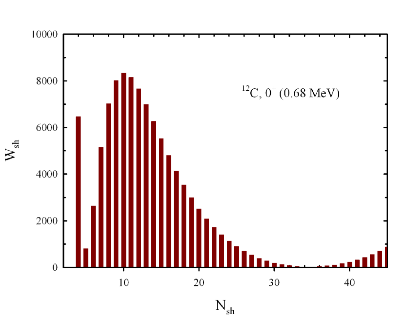
Figure 1: Weights of different oscillator shells in the wave function of the first $0^{+}$ resonance state in ¹²C.

It is interesting to compare wave function of the Hoyle state with wave functions of other resonance states in ¹²C. We selected the second $0^{+}$ resonance state and $1^{-}$ resonance state. As it follows from Table 2, the second $0^{+}$ resonance state is a broad resonance state ($\Gamma$ = 534 keV) while the $1^{-}$ resonance state is a narrow resonance state ($\Gamma$ =0.21 keV). Presented wave functions of these two states (Fig. 2) demonstrate that the wave function of narrow $1^{-}$ state has a behavior which is close to the standard behavior of the Hoyle state, as it has very large amplitudes of the oscillator shells $0\leq N_{sh}\leq 30$. Contrary to this case, the wave function of the second resonance $0^{+}$ state has rather small amplitudes of the lowest oscillator shells. It is naturally to assume that the $1^{-}$ resonance state is the Hoyle-analog state in ¹²C. We will use the standard behavior of the wave function of the Hoyle state, displayed in Fig. 1, as the additional criterion for selecting the Hoyle-analog states.

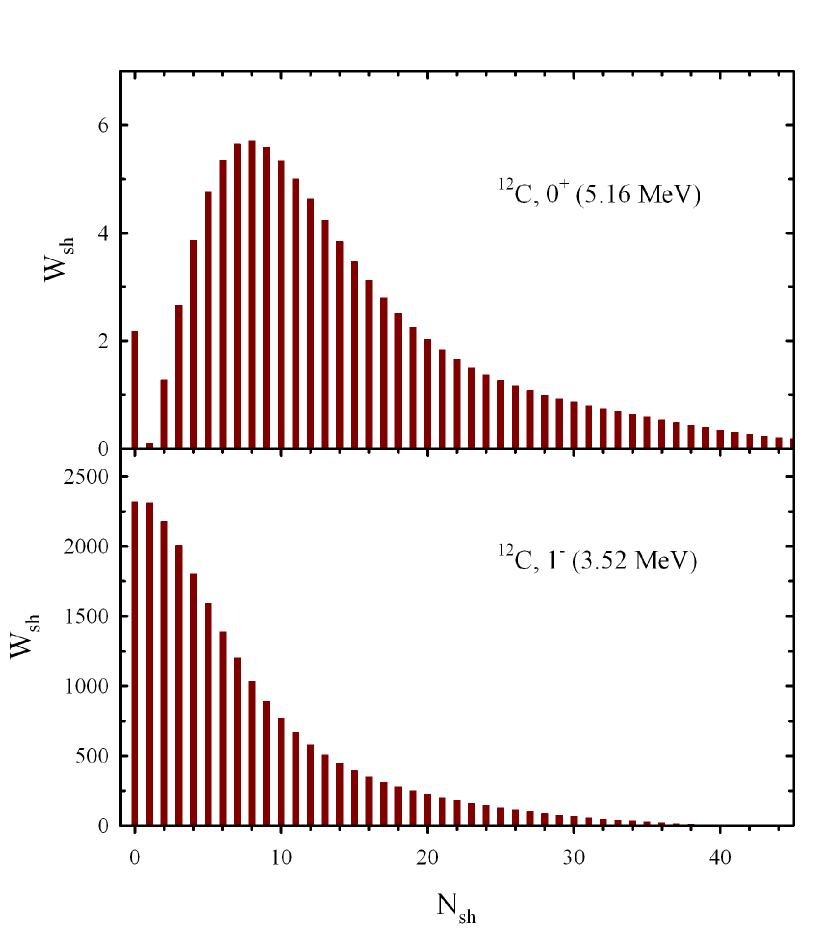
Figure 2: Structure of wave functions of the second $0^{+}$ and first $1^{-}$ resonance states in ¹²C.

In Fig. 3 we compare the resonance wave function with the wave function of the pseudo-bound state, which was calculated in the bond state approximation with $N_{\max}=70$. Both states have approximately the same energy; the energy of the resonance state is 0.536 MeV, while the pseudo-bound state has the energy 0.529 MeV.

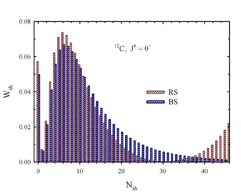
Figure 3: Comparing wave functions of the $0^{+}$ resonance state (RS) and the $0^{+}$ pseudo-bound (BS) state in ¹²C.

It is worthwhile noticing that approximately such a structure of the Hoyle state wave function has been obtained within the Complex Scaling method in Ref. Yoshida et al. (2011) and within the Fermion Molecular Dynamics in Ref. Neff and Feldmeier (2009).

We determined the shape of the triangle comprised of three alpha-particles in bound and resonance states. The average distances between clusters are displayed in Table 3.

Table 3: The energy, width and average distances $R_{1}$, $R_{2}$ between clusters for the ground states and for the $0^{+}$ and $1^{-}$ resonance states in ¹²C.

$J^{\pi}$	$E$, MeV	$\Gamma$, keV	$R_{1}$, fm	$R_{2}$, fm
$0^{+}$	-11.37	-	3.12	3.60
	0.68	2.9	6.95	8.02
	5.16	534	6.43	7.43
$1^{-}$	3.52	0.21	6.07	7.00

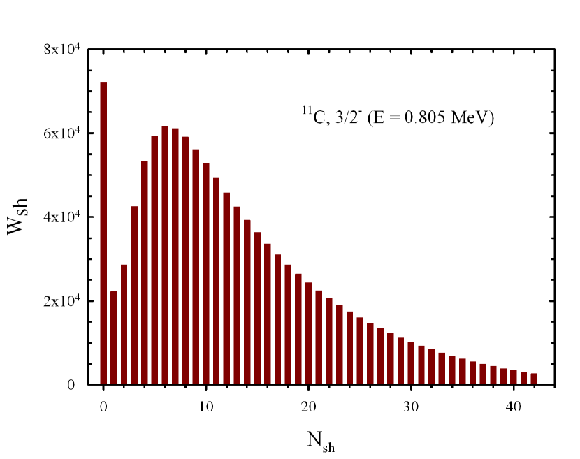
Figure 9: The shape of wave function of the 3/2^- resonance state in ¹¹C.

The shape and size of triangles for the ground and the first $0^{+}$ resonance states are consistent with the corresponding density distributions displayed in Figs. 8 and 9 of Ref. Vasilevsky et al. (2012). It is interesting to note that the shape of resonance states, shown in Table 3, is almost independent on the energy and total width of the resonance state, and the structure of resonance wave functions shown in Figs. 1 and 2. The main conclusion one may deduce from Table 3 is that the average distances between alpha-particles are rather large. The ground state of ¹²C is shows a compact three-cluster configuration, as it is expected.

Having reanalyzed properties of the Hoyle state and other resonance states in ¹²C, we suggest the following criteria for the Hoyle-analog states:

• the Hoyle-analog state is a very narrow resonance state in the three-cluster continuum;

• wave function of the Hoyle-analog state has large values of amplitudes $W_{sh}$ in the internal region.

As we pointed out above, we consider the first criterion is the most important one. We believe that the more long-lived resonance state has more chances that the system transits from a resonance state into a bound states, and vise versa. It is well-known that a resonance state could substantially increase a cross section of a processes if the total width of this resonance state is very small. To quantify the ”narrowness” of a resonance state we will calculate the ratio $\Gamma/E$. For the original Hoyle state this ratio is 2.24 $\times$ 10^-7. Such a type of resonance states are also called as the quasistationary states. As additional and important criterion we will use a behavior of the weights $W_{sh}$ of oscillator shells in the wave function of the resonance state.

Considering candidates of the Hoyle-analog states, we are also going to check other criteria formulated in Introduction.

III.2 ⁹Be and ⁹B

As was pointed out above, spectra of resonance states in ⁹Be and ⁹B have been investigated within the present model in Refs. Nesterov et al. (2014b) and Vasilevsky et al. (2017). In Ref. Vasilevsky et al. (2017) we have discovered several resonance states which can be considered as the Hoyle-analog states. For completeness of the explanation we shortly present the main results relevant to the subject of the present paper.

Energies and widths of the resonance states in ⁹Be and ⁹B presented in Ref. Vasilevsky et al. (2017) were obtained with the modified version of the Hasegawa-Nagata potential, which is often used in numerous calculations of two- and three-cluster structures of light nuclei. It was shown that our three-cluster model with such the potential reproduces fairly good spectra of resonance states in both nuclei. It was also demonstrated that the Hasegawa-Nagata potential provides a more adequate description of resonance states in ⁹Be and ⁹B, than the Minnesota potential (see detail in Ref. Nesterov et al. (2014b)).

In Table 4 we collect energies and widths of resonance states in ⁹Be and ⁹B.

Table 4: Spectra of resonance states of ⁹Be and ⁹B calculated within AMHHB model with MHNP.

9Be			9B
$J^{\pi}$	$E$, MeV	$\Gamma$, MeV	$J^{\pi}$	$E$, MeV	$\Gamma$, MeV
$3/2^{-}$	-1.574	-	$3/2^{-}$	0.379	1.08$\times$10-6
$1/2^{+}$	0.338	0.17	$1/2^{+}$	0.636	0.48
$5/2^{-}$	0.897	2.36$\times$10-5	$5/2^{-}$	2.805	0.02
$5/2^{+}$	2.086	0.11	$3/2^{+}$	2.338	2.80
$3/2_{2}^{-}$	2.704	2.53	$1/2^{-}$	3.398	3.43
$1/2^{-}$	2.866	1.60	$5/2^{+}$	3.670	0.42
$3/2^{+}$	4.062	1.22	$3/2_{2}^{-}$	3.420	3.36
$7/2^{-}$	4.766	4.04	$5/2_{2}^{-}$	5.697	5.15
$9/2^{+}$	4.913	1.27	$9/2^{+}$	6.503	2.01
$5/2_{2}^{-}$	5.365	4.38	$7/2^{-}$	6.779	0.90

There is only one very narrow resonance state in each nucleus. This is the 5/2^- resonance state in ⁹Be and the 3/2^- resonance state in ⁹B which is the ”ground state” of the nucleus. We considered these resonance states as candidates to the Hoyle-analog states. We also added the 1/2⁺ resonance state to that list of resonance states, as they lie close to the three-cluster threshold. Other resonance states in ⁹Be and ⁹B have a large total width and they were disregarded.

In Fig. 4 we display the structure of wave functions of the 5/2^- resonance states in ⁹Be and ⁹B. The total width of the 5/2^- resonance states in ⁹Be is 24 eV and amplitudes of the dominant shell weights $W_{sh}$ are of 10⁵ order of magnitude. The same resonance state in ⁹B is wider ($\Gamma$=18 keV) and thus amplitudes of the dominant shell weights $W_{sh}$ are less than 1000. As one can see that the oscillator shells with $0\leq N_{sh}<20$ give the main contribution to the wave functions of the 5/2^- resonance states. In Fig. 4 we also display $W_{sh}$ in a logarithmic scale to demonstrate their behavior in the internal region. Within the internal region, wave functions are decreasing exponentially like wave functions of bound states. Such a behavior of wave functions of the 5/2^- resonance states in ⁹Be and ⁹B allows us to consider these resonance states as the Hoyle-analog states.

In Ref. Vasilevsky et al. (2017) we have also considered the 1/2⁺ resonance states in ⁹Be and ⁹B as possible candidates to the Hoyle-analog states. These resonances lie very close to the three-cluster threshold, however, the 1/2⁺ resonance states are rather wide resonances and their wave functions both in coordinate and oscillator representations indicate a very dispersed a three-cluster configuration (see wave functions in coordinate space in Fig. 5). The later is also confirmed by the average distances $R_{1}$ and $R_{2}$.

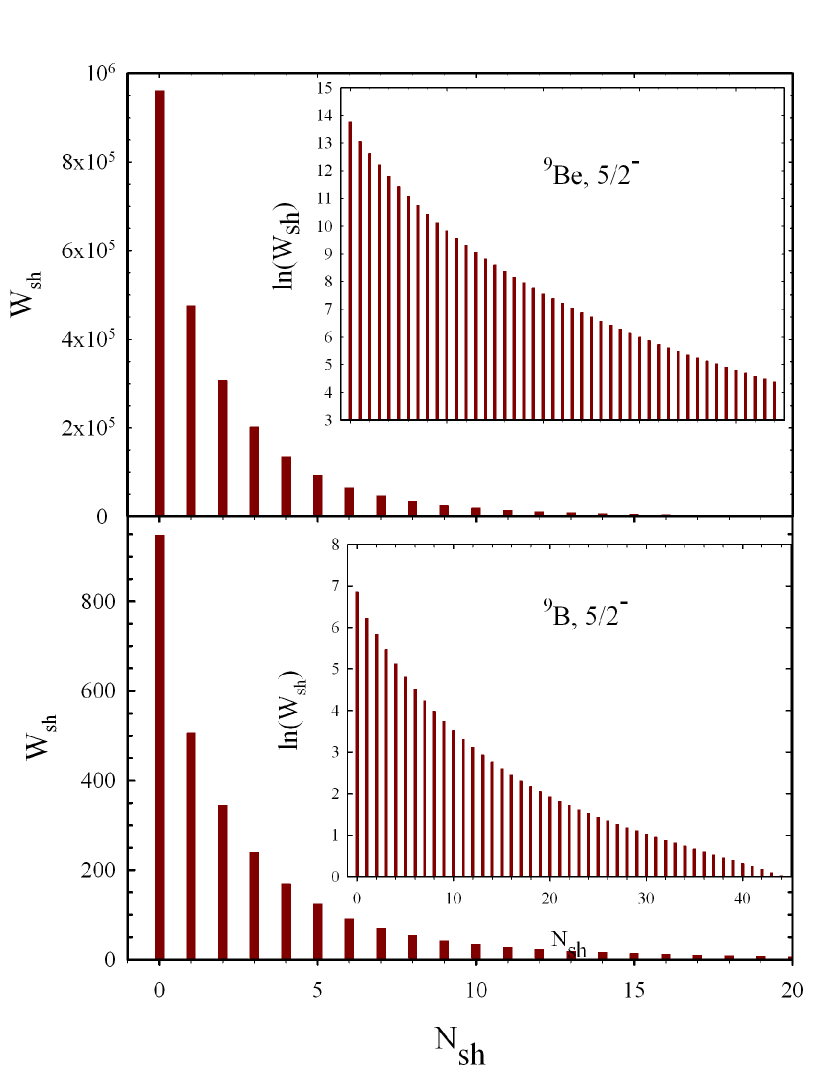
Figure 4: Weight $W_{sh}$ as a function of oscillator shell $N_{sh}$  for the 5/2^- resonance state in ⁹Be and ⁹B.

We also analyze all resonance states in ⁹Be in order to find the Hoyle-analog state. We suggested that the 5/2^- resonance state can be considered as the Hoyle-analogue state as this is a very narrow resonance state. It lives long enough and may transform to the 3/2^- ground state of ⁹Be by emitting the quadrupole gamma quanta. This reaction, which involves the triple collision of two alpha particles and neutron and a subsequent radiation of gamma quanta, can be considered as an additional way for the synthesis of the ⁹Be nuclei.

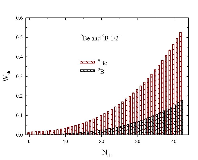
Figure 5: Weights of different oscillator shells in wave functions of the 1/2⁺ resonance states in ${}^{9}Be$ (red color) and ${}^{9}B$ (blue color).

It was shown in Ref. Vasilevsky et al. (2017) that such a behavior of the wave function (Fig. 5) is typical for a low-ling resonance state with a relatively large value of the total width.

III.3 ¹¹B and ¹¹C.

Now we consider the spectra of resonance states in ¹¹B and ¹¹C. In Table 5 we display the energy and width of resonance states in the three-cluster $\alpha+\alpha+t$ continuum of ¹¹B, which were calculated in Ref. Vasilevsky (2013).

Table 5: The spectrum of positive- and negative-parity resonance states in ¹¹B. Energy is in MeV and measured from the three-cluster $\alpha+\alpha+t$ threshold.

$J^{\pi}$	$E$, MeV	$\Gamma$, keV	$J^{\pi}$	$E$, MeV	$\Gamma$, keV
$3/2^{-}$	0.755	0.58	$1/2^{+}$	0.437	15.26
	1.402	185.18		0.702	12.30
	1.756	143.72		1.597	15.95
$1/2^{-}$	1.436	374.64	$3/2^{+}$	1.147	1.498
	1.895	100.95		1.367	8.58
	2.404	450.07		1.715	41.24
$5/2^{-}$	0.583	5.14$\times$10-4	$5/2^{+}$	1.047	1.54
	1.990	32.63		1.951	40.20
	2.251	138.87		2.265	54.73
	2.905	120.46		2.748	167.61
$7/2^{-}$	1.591	4.14	$7/2^{+}$	1.076	2.04$\cdot$10-2
	1.778	3.04		2.119	26.32
	2.471	20.18		2.536	100.47

In a small range of energies $0<E<3$ MeV we observed 26 resonance states. The large part of these resonances are narrow resonance states with the total width less than 50 keV. The similar picture is observed in ¹¹C. The energy and width of positive- and negative-parity states are shown in Table 6. Details of these calculations can be found in Ref. Vasilevsky (2013).

Table 6: The spectrum of positive- and negative-parity resonance states in ${}^{11}C$. Energy is in MeV and measured from three-cluster $\alpha+\alpha+^{3}$He threshold.

$J^{\pi}$	$E$, MeV	$\Gamma$, keV	$J^{\pi}$	$E$, MeV	$\Gamma$, keV
$3/2^{-}$	0.805	9.93$\times$10-3	$1/2^{+}$	0.906	162.94
	1.920	105.08		1.930	59.88
	2.324	619.76		2.679	86.69
$1/2^{-}$	1.142	0.708	$3/2^{+}$	2.268	34.25
	2.266	790.98		2.478	159.28
	3.014	366.15		2.850	115.19
$5/2^{-}$	0.783	9.64$\times$10-5	$5/2^{+}$	1.460	0.90
	1.897	5.77		2.346	82.72
	3.026	182.69		3.179	122.75
	3.491	392.96	$7/2^{+}$	1.765	7.40$\cdot$10-2
$7/2^{-}$	2.700	66.63		2.542	8.19
	3.538	21.18		3.237	119.13

By using the criteria for selecting the candidate to the Hoyle-analog states, formulated above, we selected four resonance states in ¹¹B and four resonance states in ¹¹C. In Table 7 we display the properties of the selected resonance states in ¹¹B and ¹¹C, and compare them with some bound states. We did not include the 1/2⁺ resonance state in ¹¹C as it has a relatively large total width.

Table 7: Parameters of resonance states in ¹¹B and ¹¹C selected as candidates to the Hoyle-analog states. The average distances $R_{1}$ and $R_{2}$ are presented both for resonance states and for bound states.

Nucleus	$J^{\pi}$	$E$, MeV	$\Gamma$, keV	$\Gamma/E$	$R_{1}$, fm	$R_{2}$, fm
	$3/2^{-}$	-11.055			2.60	2.88
	$3/2^{-}$	-5.667			2.90	3.38
	$3/2^{-}$	-0.589			4.83	6.79
11B	$1/2^{+}$	0.437	15.26	3.49$\times$10-2	10.48	6.77
	$5/2^{-}$	0.583	5.14$\times$10-4	8.81$\times$10-7	4.71	7.20
	$3/2^{-}$	0.755	0.58	7.7$\times$10-4	5.36	7.75
	$5/2^{+}$	1.047	1.54	1.47$\times$10-3	4.98	7.47
	$3/2^{-}$	-9.073			2.64	2.90
	$3/2^{-}$	-3.835			2.97	3.43
	$1/2^{+}$	0.906	162.94		10.75	7.08
11C	$5/2^{-}$	0.783	9.64$\times$10-5	1.23$\times$10-7	3.20	3.87
	$3/2^{-}$	0.805	9.93$\times$10-3	1.23$\times$10-5	5.02	6.86
	$5/2^{+}$	1.460	0.90	6.16$\times$10-4	5.00	6.69

Figs. 6 and 7 demonstrating wave functions of the 5/2^- resonance states in ¹¹B and ¹¹C explicitly indicate that these resonance states can be considered as the Hoyle analog state. Both resonance states have very large amplitudes of weights $W_{sh}$. Structure of the wave functions of the 5/2^- resonance states in ¹¹C looks like as a wave function of a bound state. These results also show that the average distances between clusters $R_{1}$ and $R_{2}$ in these resonance states are very close to average distances for bound states, for instance, for the first excited 3/2^- state in ¹¹C. From the average distances $R_{1}$ and $R_{2}$ for the resonance states in ¹¹B and ¹¹C in Table 7, we see that the most narrow 5/2^- resonance states in ¹¹C has the most compact configuration of three clusters. Contrary to this resonance state, the narrowest 5/2^- resonance states at $E$=0.583 MeV in ¹¹B, the total width of which is five time larger than the width of the 5/2^- resonance states in ¹¹C, has rather dispersed structure with the average distance between alpha particles equals to 7.2 fm.

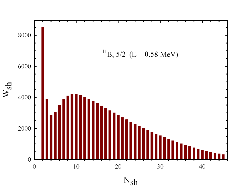
Figure 6: Weights of oscillator shells in the wave functions of the 5/2^- resonance state ($E$=0.58 MeV $\Gamma$=0.5 eV) in ¹¹B.

Figure 7: Structure of the wave function of the very narrow 5/2^- resonance state in ¹¹C.

It is interesting to note that the Coulomb interaction makes the 5/2^- resonance state in ¹¹C more narrower than that in ¹¹B. As one may expect, it also increase the energy of the resonance in ¹¹C comparing to its position in ¹¹B. The same picture is observed for the 3/2^- resonance states in ¹¹B and ¹¹C. Larger the Coulomb barrier in ¹¹C leads to the very large amplitudes of $W_{sh}$ for the 3/2^- resonances state. One can compare amplitudes of $W_{sh}$ for 3/2^- resonance states in ¹¹B and ¹¹C in Figs. 8 and 9, respectively.

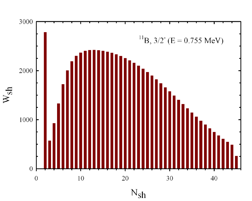
Figure 8: The shape of the wave function of the 3/2^- resonance state in ¹¹B.

We do not show wave functions of the 1/2⁺ resonance states in ¹¹B and ¹¹C here as they are very similar to the wave functions of these resonance states in ⁹Be and ⁹B. Moreover, the shape of three-cluster triangles in those pairs of nuclei is also similar.

As we pointed out in Introduction, there are few publications which devoted to the Hoyle-analog states in ¹¹B and ¹¹C. In Refs. Kanada-En’yo (2007) and Kanada-En’yo et al. (2011), the spectra of ¹¹B and ¹¹C have been obtained within the antisymmetrized molecular dynamics (AMD). The excited states have been treated as bound states, it mean that the widths and energies of these states with respect to the three-cluster thresholds were not determined. By analyzing the probability of electromagnetic transitions, authors came to the conclusion that the 3/2^- excited states have a dilute cluster structure $\alpha+\alpha+t$ and $\alpha+\alpha+^{3}$He, and thus can be considered as the Hoyle-analog states. It was also claimed by the authors, that the 5/2^- states have no a well-developed cluster structure and therefore cannot be considered as the Hoyle-analog states.

In Refs. Yamada and Funaki (2010) and Yamada and Funaki (2012) resonance states in two- and three-body continuum of ¹¹B and ¹¹C have been determined with the complex scaling method. The 3/2^- resonance state is located bellow the $\alpha+\alpha+t$ threshold has a compact cluster configuration, as was shown by the authors of Refs. Yamada and Funaki (2010, 2012), and therefore was not considered as a candidate to the Hoyle-analog states. The wave function of the 1/2⁺ resonance state which has ”the gas-like structure with a large nuclear radius”, as stressed by the authors, and thus can be considered as the Hoyle-analog state. It is interesting to note that the parameters ($E$=0.75 MeV, $\Gamma$=190 keV) of the 1/2⁺ resonance state, determined in Refs. Yamada and Funaki (2010, 2012), are rather different to those ($E$=0.44 MeV, $\Gamma$=15 keV) displayed in the present paper. This difference can be ascribed to the different types of nucleon-nucleon potentials involved in these two calculations. The 1/2⁺ resonance state, obtained in our calculations, has also a large nuclear radius, however is not considered as the Hoyle-analog state in our criterion.

III.4 ¹⁰B

In Table 8 we show the three-cluster resonance states in ¹⁰B calculated with the MP. Details of these calculations can be found in Ref. Nesterov et al. (2014a), where the spectrum of bound states of ¹⁰B has been discussed. Here, we use the same input parameters to calculate spectrum of resonance states in the three-cluster $\alpha+\alpha+d$ continuum. As we can see in Table 8, there are a few narrow resonance states which can be considered as the Hoyle-analog states. Three resonance states have the total width less than 12 keV and the ratio $\Gamma/E$ does not exceed 11.5$\times$10^-3.

Table 8: Parameters of resonance states in ${}^{10}B$. The average distances $R_{1}$ and $R_{2}$ are calculated for the candidates to the Hoyle-analog states.

$J^{\pi}$	$E$, MeV	$\Gamma$, keV	$\Gamma/E$	$R_{1}$, fm	$R_{2}$, fm
$1^{+}$	0.604	232.30	0.384
	0.987	7.08	7.17$\times$10-3	6.67	10.67
	1.536	196.36	0.128
$2^{+}$	1.055	12.063	11.43$\times$10-3	6.64	10.83
	2.810	170.74	60.76$\times$10-3
$3^{+}$	1.062	11.73	11.05$\times$10-3	6.43	10.35
	2.202	526.47	0.239
$1^{-}$	1.100	76.75	69.77$\times$10-3	9.31	10.84
	1.820	562.71	0.309

In Table 8 we also show the average distances between interacting clusters. It is necessary to recall that $R_{2}$ stands for the distance between two alpha-particles, and $R_{1}$ denotes the distance between the deuteron and the center of mass of two alpha-particles. It is interesting to compare the average distance between clusters for resonance states with those for the bound states. For the ground $3^{+}$ state we have obtained $R_{1}$ =2.60 fm and $R_{2}$ = 3.10 fm. This is a compact configuration despite that the binding energy is -5.95 MeV, accounted from the three-cluster threshold $\alpha+\alpha+d$, is not very small. The first excited $3^{+}$ state is a weakly bound state as its energy is -0.95 MeV, however it is also a rather compact configuration with the average distances $R_{1}$ = 4.07 and $R_{1}$ = 5.35 fm. As we see in Table 8, all resonance states selected as the candidates to the Hoyle-analog states have a dispersed configuration with a large distance between alpha particles.

Let us turn our attention to the wave functions of the selected resonance states. In Fig. 10 we display shell weights in wave functions of the narrow $3^{+}$ and $1^{+}$ resonance states in ¹⁰B. These resonance state have the smallest total width among all resonances in ¹⁰B. One notices, that the compact three-cluster configuration ($N_{sh}$ =0) has a relatively large contribution to these wave functions. The shapes of the curves are similar to the shape of the Hoyle state (Fig. 1), however the amplitudes are much more smaller.

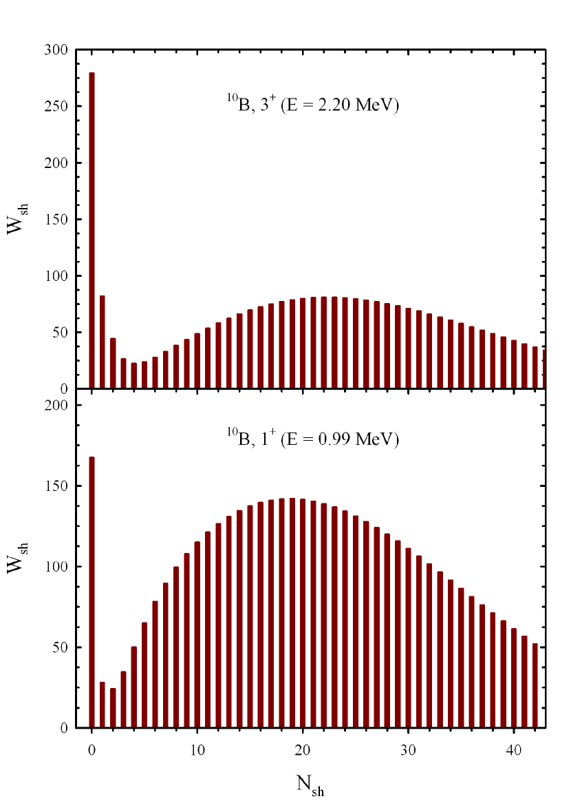
Figure 10: Weights of different oscillator shells in wave functions of the $3^{+}$ and $1^{+}$ resonance states in ¹⁰B.

We assume that the interplay of the attractive potential, created by the central and spin-orbital parts of the nucleon-nucleon interaction, and repulsive potential, formed by the Coulomb interaction, does not create a favorable situation for very narrow resonance states in ¹⁰Be.

IV Conclusion

We have performed a systematic investigation of the three-cluster resonance states in light nuclei ⁹Be, ⁹B, ¹⁰B, ¹¹B, ¹¹C and ¹²C. These nuclei have been considered to have a three-cluster structure composed of two alpha particles and an $s$-shell nucleus. A microscopic three-cluster model was applied to search and to study resonance states embedded in the three-cluster continuum. This model imposes proper boundary conditions by employing hyperspherical coordinates and hyperspherical harmonics. Having reanalyzed properties of the Hoyle state, we formulated criteria for the Hoyle-analog states. Among these resonances, we have found the Hoyle-analog states in these nuclei. The Hoyle-analog states are created by a collision of two alpha-particles and a neutron, proton, triton and nucleus ³He. These resonance states have very small width. We discussed an alternative way for the synthesis of light nuclei in a triple collision, in the same manner as was suggest by F. Hoyle for ¹²C. We found several resonance states having the total width of a few eV. Most of the obtained resonance states have the width of few dozens of keV.

In Table 9 we collect the parameters of the Hoyle-analog states in light nuclei under consideration. Results presented in this Table allow us to formulate the new criteria for selecting the Hoyle-analog states. A three-cluster resonance state can be treated as the Hoyle-analog state if the ratio $E/\Gamma<$ 2$\times$10^-3 for this resonance state.

Figure 11 visualizes the results presented in Table 9. This figure explicitly demonstrates effects of the Coulomb interaction on the energy of three-cluster resonance states in mirror nuclei ⁹Be and ⁹B and ¹¹B and ¹¹C. One can see that the Coulomb interaction has a more stronger impact on the position of the 5/2^- resonance states in ⁹Be and ⁹B than on the position of the 3/2^-, 5/2^- and 5/2⁺ resonance states in ¹¹B and ¹¹C.

Table 9: Parameters of the Hoyle-analog states in light nuclei ⁹Be, ⁹B, ¹¹B and ¹¹C.

Nucleus	Configuration	$J^{\pi}$	$E$, MeV	$\Gamma$, keV	$\Gamma/E$
${}^{9}Be$	$\alpha+\alpha+n$	$5/2^{-}$	0.897	2.36$\cdot$10-2	2.63$\cdot$10-5
${}^{9}B$	$\alpha+\alpha+n$	$3/2^{-}$	0.379	1.08$\cdot$10-3	2.84$\cdot$10-6
		$5/2^{-}$	2.805	18.0$\cdot$10-3	6.42$\cdot$10-6
${}^{11}B$	$\alpha+\alpha+^{3}H$	$5/2^{-}$	0.583	5.14$\cdot$10-4	8.87$\cdot$10-7
		$3/2^{-}$	0.755	0.58	7.70$\times$10-4
		$5/2^{+}$	1.047	1.54	1.47$\times$10-3
${}^{11}C$	$\alpha+\alpha+^{3}He$	$5/2^{-}$	0.783	9.64$\cdot$10-5	1.23$\cdot$10-7
		$3/2^{-}$	0.805	9.93$\cdot$10-3	1.23$\cdot$10-5
		$5/2^{+}$	1.460	0.90	6.16$\times$10-4

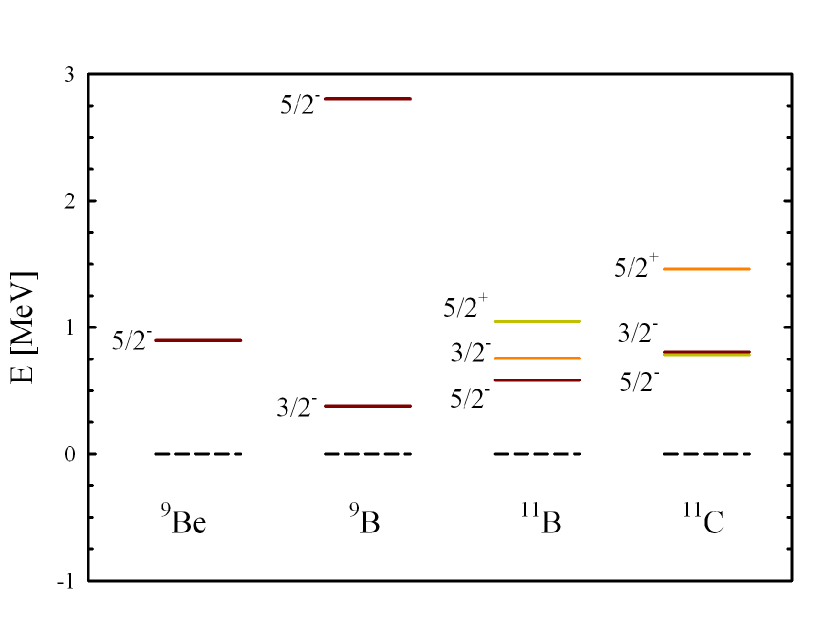
Figure 11: Spectrum of the Hoyle-analog states in ⁹Be, ⁹B, ¹¹B and ¹¹C.

In Table 10 we collect all resonance states for the total momentum $J$ and positive parity, where the zero value of the total orbital momentum ($L=0$) is dominant. This is the case for ⁹Be, ⁹B, ¹¹B and ¹¹C. The continuous spectrum states with $L=0$ can be interpreted as a head-on collision of the third cluster with the ⁸Be nucleus being in the $0^{+}$ state. As one can see, all these resonance states lie rather close to the three-cluster threshold and they are fairly wide, as the total widths are $\Gamma$=15 keV and more. Therefor they cannot be considered as the Hoyle-analog states.

Table 10: The energy and width of resonance states which are created by the three-cluster configuration with the total orbital momentum $L=0$.

Nucleus	$J^{\pi}$	$E$, MeV	$\Gamma$, keV
9Be	$1/2^{+}$	0.338	168
9B	$1/2^{+}$	0.636	477
10B	$1^{+}$	0.604	232
11B	$1/2^{+}$	0.437	15
11C	$1/2^{+}$	0.906	163

Figures 12, 13 and 14 of average distances $R_{1}$ and $R_{2}$ demonstrate the most probable shapes of triangles of three-cluster resonance states in ⁹Be, ¹¹B and ¹¹C, respectively. In all these Figures we also show the triangle comprised by three alpha-particles in the Hoyle resonance state in ¹²C. The 1/2⁺ resonance states in ⁹B, ¹¹B and ¹¹C has very large triangles where a neutron, triton and ³He nucleus are far away from two alpha-particles. The Hoyle-analog states in these nuclei have a triangle comparable with the shape of the Hoyle-state and in some cases (for example, for $J^{\pi}$ = 5/2^-) they are more compact.

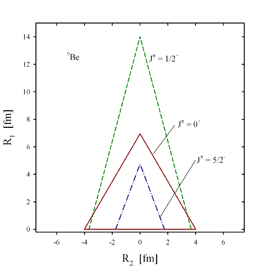
Figure 12: Shape of triangles for some selected resonance states in ⁹Be and the Hoyle state ($J^{\pi}=0^{+}$).

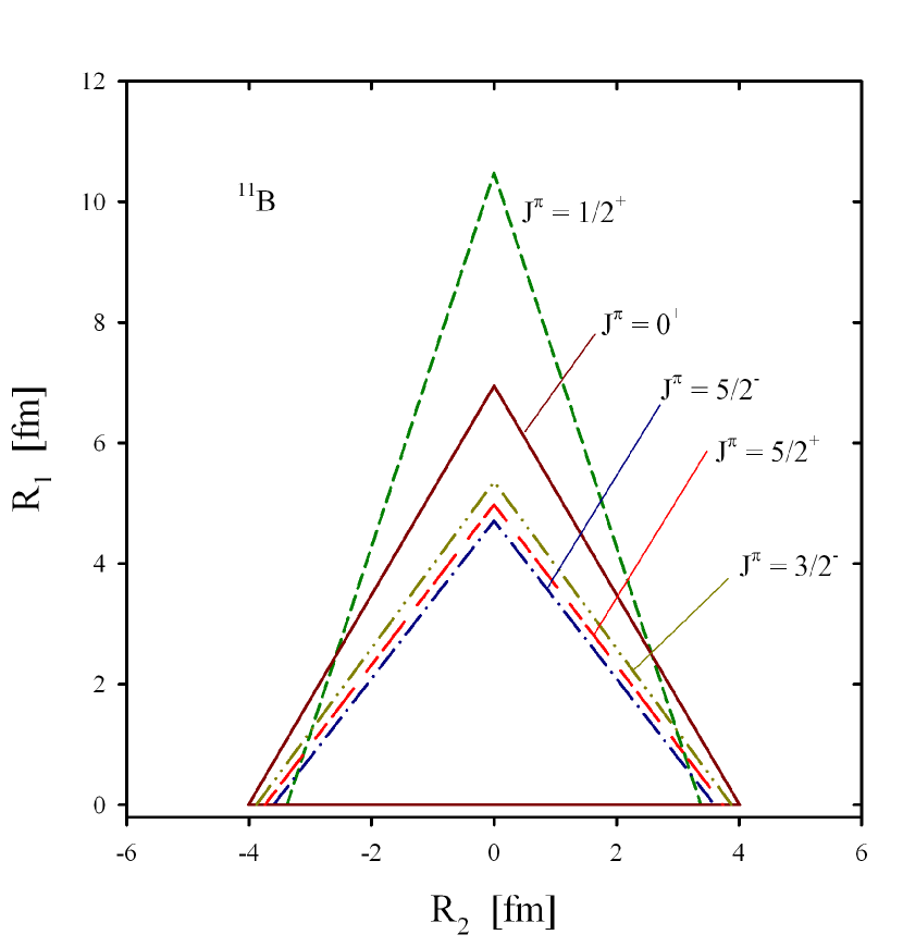
Figure 13: Shape of triangles of some resonance states in ¹¹B and the Hoyle resonance state ($J^{\pi}=0^{+}$).

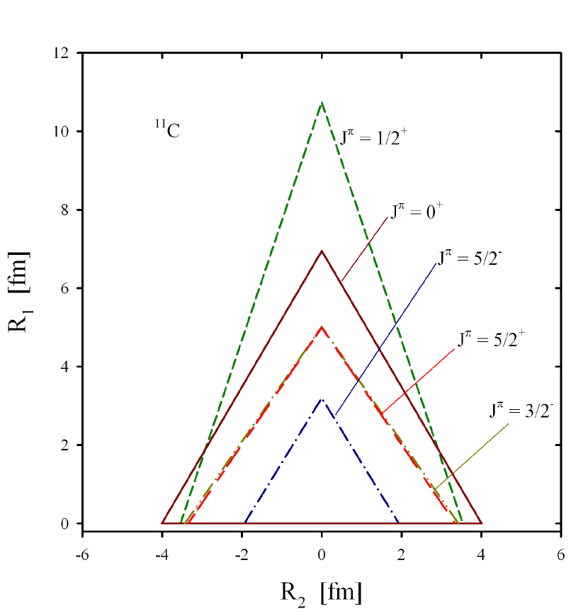
Figure 14: Shape of triangles of some resonance states in ¹¹C compared to the Hoyle resonance state ($J^{\pi}=0^{+}$).

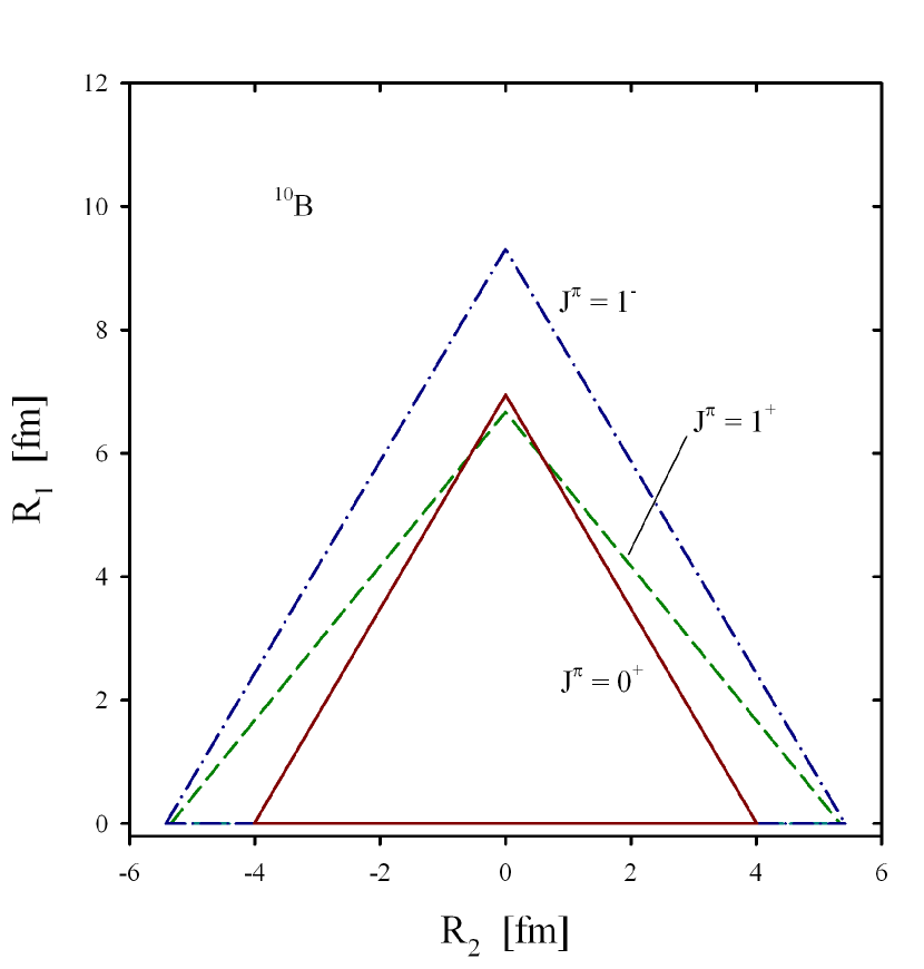
Figure 15: The most probable shape of three-cluster triangles for most narrow resonance states in ¹⁰B and compared with the Hoyle state ($J^{\pi}=0^{+}$).

Figure 15 demonstrates the shape of triangles for resonance states in ¹⁰B. They are the narrowest resonance states, however the amplitudes of $W_{sh}$, as was shown above, are fairly small and the ratios $E/\Gamma$ for these states are large. They don’t match our criteria for the Hoyle-analog states. As we see, the distance between alpha-particles is greater than this distance in the $0^{+}$ resonance state in ¹²C and all other nuclei considered in the present paper. To this end, the 1/2⁺ resonance states in ⁹Be, ⁹B, ¹¹B and ¹¹C which are considered as candidates to the Hoyle states and did not match our criteria, have the average distance between two alpha-particles comparable with the Hoyle state, meanwhile the average distance of the third cluster (neutron, proton, triton and ³He, respectively) to the center of mass of two alpha particles is very large.

References

- Hoyle (1954) F. Hoyle, Astrophys. J. Suppl. 1, 121 (1954).
- Cook et al. (1957) C. W. Cook, W. A. Fowler, C. C. Lauritsen, and T. Lauritsen, Phys. Rev. 107, 508 (1957).
- J. H. Kelley and J. E. Purcell and C. G. Sheu (2017) J. H. Kelley and J. E. Purcell and C. G. Sheu, Nucl. Phys. A 968, 71 (2017), ISSN 0375-9474.
- Freer and Fynbo (2014) M. Freer and H. O. U. Fynbo, Prog. Part. Nucl. Phys. 78, 1 (2014).
- Bethe (1939) H. A. Bethe, Phys. Rev. 55, 434 (1939).
- Kanada-En’yo (2007) Y. Kanada-En’yo, Phys. Rev. C 75, 024302 (2007).
- Yamada and Funaki (2010) T. Yamada and Y. Funaki, Phys. Rev. C 82, 064315 (2010).
- Kanada-En’yo et al. (2011) Y. Kanada-En’yo, T. Suhara, and F. Kobayashi, J. Phys. Conf. Ser. 321, 012009 (2011).
- Suhara and Kanada-En’yo (2012) T. Suhara and Y. Kanada-En’yo, Phys. Rev. C 85, 054320 (2012).
- Yamada and Funaki (2012) T. Yamada and Y. Funaki, Progr. Theor. Phys. Suppl. 196, 388 (2012).
- Kanada-En’yo and Suhara (2015) Y. Kanada-En’yo and T. Suhara, Phys. Rev. C 91, 014316 (2015).
- Zhou and Kimura (2017) B. Zhou and M. Kimura, ArXiv e-prints (2017), eprint 1711.04439.
- Chiba and Kimura (2018) Y. Chiba and M. Kimura, ArXiv e-prints (2018), eprint 1801.00562.
- Vasilevsky et al. (2001a) V. Vasilevsky, A. V. Nesterov, F. Arickx, and J. Broeckhove, Phys. Rev. C 63, 034606 (16 pp) (2001a).
- Vasilevsky et al. (2012) V. Vasilevsky, F. Arickx, W. Vanroose, and J. Broeckhove, Phys. Rev. C 85, 034318 (2012).
- Vasilevsky et al. (2017) V. S. Vasilevsky, K. Katō, and N. Z. Takibayev, Phys. Rev. C 96, 034322 (2017).
- Vasilevsky (2013) V. S. Vasilevsky, Ukr. J. Phys. 58, 544 (2013).
- Nesterov et al. (2014a) A. V. Nesterov, V. S. Vasilevsky, and T. P. Kovalenko, Ukr. J. Phys. 59, 1065 (2014a).
- Vasilevsky et al. (2001b) V. Vasilevsky, A. V. Nesterov, F. Arickx, and J. Broeckhove, Phys. Rev. C 63, 034607 (7 pp) (2001b).
- Broeckhove et al. (2007) J. Broeckhove, F. Arickx, P. Hellinckx, V. S. Vasilevsky, and A. V. Nesterov, J. Phys. G Nucl. Phys. 34, 1955 (2007).
- Nesterov et al. (2010) A. V. Nesterov, F. Arickx, J. Broeckhove, and V. S. Vasilevsky, Phys. Part. Nucl. 41, 716 (2010).
- Nesterov et al. (2014b) A. V. Nesterov, V. S. Vasilevsky, and T. P. Kovalenko, Phys. Atom. Nucl. 77, 555 (2014b).
- Zickendraht (1965) W. Zickendraht, Ann. Phys. 35, 18 (1965).
- A. Avery (1989) A. Avery, Hyperspherical Harmonics. Applications in quantum theory (Kluwer, Dordrecht, 1989).
- R. I. Dzhibuti, N. B. Krupennikova (1984) R. I. Dzhibuti, N. B. Krupennikova, The Method of Hyperspherical Functions in the Quantum Mechanics of Several Bodies (in Russian) (Metsniereba, Tbilisi, 1984).
- Zernike and Brinkman (1935) F. Zernike and H. C. Brinkman, Proc. Kon. Acad. Wetensch. Amsterdam 38, 161 (1935).
- Abramowitz and Stegun (1972) M. Abramowitz and A. Stegun, Handbook of Mathematical Functions (Dover Publications, Inc., New-York, 1972).
- Tang et al. (1978) Y. C. Tang, M. Lemere, and D. R. Thompsom, Phys. Rep. 47, 167 (1978).
- Vasilevsky et al. (2018) V. S. Vasilevsky, Y. A. Lashko, and G. F. Filippov, Phys. Rev. C 97, 064605 (2018).
- Thompson et al. (1977) D. R. Thompson, M. LeMere, and Y. C. Tang, Nucl. Phys. A286, 53 (1977).
- Reichstein and Tang (1970) I. Reichstein and Y. C. Tang, Nucl. Phys. A 158, 529 (1970).
- Hasegawa and Nagata (1971) A. Hasegawa and S. Nagata, Prog. Theor. Phys. 45, 1786 (1971).
- Tanabe et al. (1975) F. Tanabe, A. Tohsaki, and R. Tamagaki, Prog. Theor. Phys. 53, 677 (1975).
- Kurokawa and Katō (2007) C. Kurokawa and K. Katō, Nucl. Phys. A 792, 87 (2007).
- Yoshida et al. (2011) T. Yoshida, N. Itagaki, and K. Katō, Phys. Rev. C 83, 024301 (2011).
- Neff and Feldmeier (2009) T. Neff and H. Feldmeier, Few-Body Syst. 45, 145 (2009).