Fully Convolutional Networks with Sequential Information
for Robust Crop and Weed Detection in Precision Farming

Abstract

Reducing the use of agrochemicals is an important component towards sustainable agriculture. Robots that can perform targeted weed control offer the potential to contribute to this goal, for example, through specialized weeding actions such as selective spraying or mechanical weed removal. A prerequisite of such systems is a reliable and robust plant classification system that is able to distinguish crop and weed in the field. A major challenge in this context is the fact that different fields show a large variability. Thus, classification systems have to robustly cope with substantial environmental changes with respect to weed pressure and weed types, growth stages of the crop, visual appearance, and soil conditions.

In this paper, we propose a novel crop-weed classification system that relies on a fully convolutional network with an encoder-decoder structure and incorporates spatial information by considering image sequences. Exploiting the crop arrangement information that is observable from the image sequences enables our system to robustly estimate a pixel-wise labeling of the images into crop and weed, i.e. , a semantic segmentation. We provide a thorough experimental evaluation, which shows that our system generalizes well to previously unseen fields under varying environmental conditions—a key capability to actually use such systems in precision framing. We provide comparisons to other state-of-the-art approaches and show that our system substantially improves the accuracy of crop-weed classification without requiring a retraining of the model.

I Introduction

A sustainable agriculture is one of the seventeen sustainable development goals of the United Nations. A key objective is to reduce the reliance on agrochemicals such as herbicides or pesticides due to its side-effects on the environment, biodiversity, and partially human health. Autonomous precision farming robots have the potential to address this challenge by performing targeted and plant-specific interventions in the field. These interventions can be selective spraying or mechanical weed stamping, see Fig. 1. A crucial prerequisite for selective treatments through robots is a plant classification system that enables robots to identify individual crop and weed plants in the field. This is the basis for any following targeted treatment action [1, 2].

Several vision-based learning methods have been proposed in the context of crop and weed detection [3, 4, 5, 6, 7, 8]. Typically, such methods are based on supervised learning methods and report high classification performances in the order of $80$-$95$% in terms of accuracy. However, we see a certain lack in the evaluation of several methods with respect to the generalization capabilities to unseen situations, i.e., the classification performance under substantial changes in the plant appearance and soil conditions between training and testing phase. This generalization capabilities to new fields, however, is essential for actually deploying precision farming robots with selective intervention capabilities. Also Slaughter et al.  [9] conclude in their review about robotic weed control systems that the missing generalization capabilities of the crop-weed classification technology is a major problem with respect to the deployment and commercialization of such systems. Precision farming robots need to operate in different fields on a regular basis. Thus, it is crucial for the classification system to provide robust results under changing conditions such as differing weed density and weed types as well as appearance, growth stages of the plants, and finally soil conditions and types. Purely visual crop-weed classification systems often degrade due to such environmental changes as these correlate with the underlying data distribution of the images.

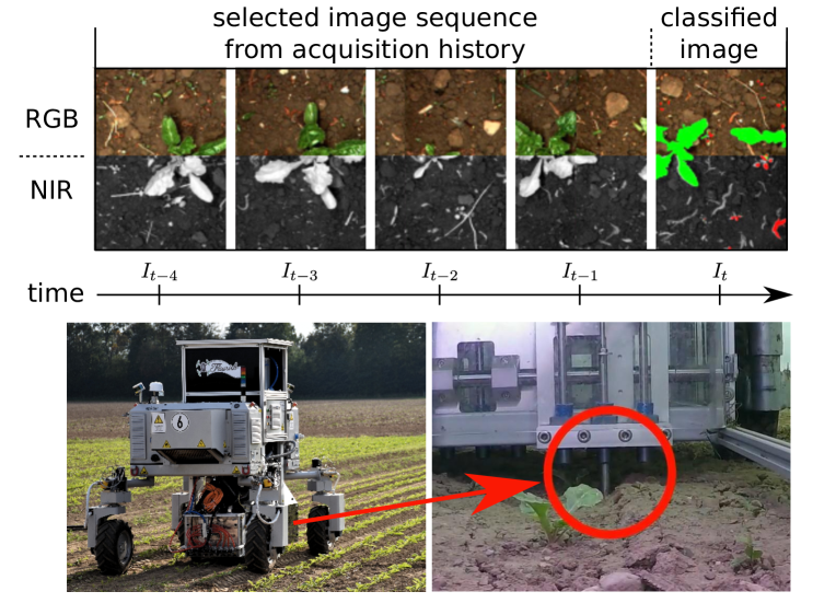
Figure 1: The image depicts the BoniRob platform perceiving RGB+NIR images along the crop row as well as crop-weed classification results by exploiting the repetitive plant arrangement information. Our approach analyzes image sequences from the acquisition history and provides a pixel-wise image labeling of the field under the robot. The lower right image shows a mechanical actuator stamping the detected weeds into the ground.

In this work, we aim at overcoming the performance loss in crop-weed detection due to changes in the underlying distribution of the image data. To achieve that, we exploit geometric patterns that result from the fact that several crops are sowed in rows. Within a field of row crops (such as sugar beets or corn), the plants share a similar lattice distance along the row, whereas weeds appear more randomly. In contrast to the visual cues, this geometric signal is much less affected by changes in the visual appearance. Thus, we propose an approach to exploit this information as an additional signal by analyzing image sequences that cover a local strip of the field surface in order to improve the classification performance. Fig. 1 depicts the employed farming robot during operation in the field and an example of an image sequence consisting of 4-channel images, i.e., conventional red, green, and blue (RGB) channels as well as an additional near infra-red (NIR) channel.

The main contribution of this work is a novel, vision-based crop-weed classification approach that operates on image sequences. Our approach performs pixel-wise semantic segmentation of images into soil, crop, and weed. Our proposed method is based on a fully convolutional network (FCN) with an encoder-decoder structure and incorporates information about the plant arrangement by a novel extension. This extension, called sequential module, enables the usage of image sequences to implicitly encode the local geometry. This combination leads to better generalization performance even if the visual appearance or the growth stage of the plants changes between training and test time. Our system is trained end-to-end and relies neither on pre-segmentation of the vegetation nor on any kind of handcrafted features.

We make the following two key claims about our approach. First, it generalizes well to data acquired from unseen fields and robustly classifies crops at different growth stages without the need for retraining (we achieve an average recall of more than $94$% for crops and over $91$% for weeds even in challenging settings). Second, our approach is able to extract features about the spatial arrangement of the plantation from image sequences and can exploit this information to detect crops and weeds solely based on geometric cues. These two claims are experimentally validated on real-world datasets, which are partially publicly available [10]. We compare our approach to other state-of-the-art approaches and to a non-sequential FCN model. Through simulations, we furthermore demonstrate the approach’s ability to learn plant arrangement information. We plan to publish our code.

II Related Work

While there has recently been significant progress towards robust vision-based crop-weed classification, many systems rely on handcrafted features [3, 11, 4]. However, the advent of convolution neural networks (CNN) also spurred increasing interest in end-to-end crop-weed classification systems [12, 13, 14, 5, 6, 8] to overcome the inflexibility and limitations of handcrafted vision pipelines.

In this context, CNNs are often applied in pixel-wise fashion operating on image patches provided by a sliding window approach. Using this principle, Potena et al.  [8] use a cascade of CNNs for crop-weed classification, where the first CNN detects vegetation and then only the vegetation pixels are classified by a deeper crop-weed CNN. McCool et al.  [13] fine-tune a very deep CNN [15] and attain practical processing times by compression of the fine-tuned network using a mixture of small, but fast networks, without sacrificing too much classification accuracy.

Fully convolutional networks (FCN) [16] directly estimate a pixel-wise segmentation of the complete image and can therefore use information from the whole image. The encoder-decoder architecture of SegNet [17] is nowadays a common building block of semantic segmentation approaches [18, 19]. Sa et al. [20] propose to use the SegNet architecture for multi-spectral crop-weed classification from a micro aerial vehicle. Milioto et al.  [5] use a similar architecture, but combine RGB images with background knowledge encoded in additional input channels.

All systems share the need for tedious re-labeling effort to generalize to a different field. To alleviate this burden, Wendel and Underwood [21] enable self-supervised learning by exploiting plant arrangement in rows. Recently, we [22] proposed to exploit the plant arrangement to re-learn a random forest with minimal labeling effort in a semi-supervised way. Hall et al.  [23] minimize the labeling effort through an unsupervised weed scouting process [24] that clusters visually similar images and allows to assign labels only to a small number of candidates to label the whole acquired data. Cicco et al. [12] showed that a SegNet-based crop-weed segmentation can be learned using only synthetic images.

In contrast to the aforementioned prior work, we combine a FCN with sequential information to exploit the repetitive structure of the plant arrangement leading to better generalization performance without re-labeling effort. To the best of our knowledge, we are therefore the first to propose an end-to-end learned semantic segmentation approach exploiting the spatial arrangement of row plants.

III Sequential Crop-weed Classification System

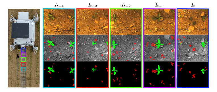
Figure 2: Left: BoniRob acquiring images while driving along the crop row. Our approach exploits an image sequence by selecting those image from the history that do not overlap in object space. Right: Exemplary prediction of crop and weed for an image sequence captured on a field near Stuttgart where the classification model was solely trained on data acquired in Bonn; top row: RGB images; middle row: predicted label mask projected on the NIR image (crop in green, weed in red, background transparent); bottom row: ground truth.

The primary objective of our approach is to enable robots to robustly identify crops and weeds during operation in the field, even when the visual appearance of the plants and soil has changed. We propose a sequential FCN-based classification model for pixel-wise semantic segmentation of the classes (i) background, i.e. mostly soil, (ii) crops (sugar beet), and (iii) weeds. The key idea is to exploit information about the plant arrangement, which is given by the planting process. We let the classification model learn this information from image sequences representing a part of the crop row and fuse the arrangement information with visual features. With this novel combination, we can improve the performance and generalization capabilities of our classification system.

Fig. 2 depicts the $S=5$ selected RGB+NIR images for building the sequence $\mathcal{I}=\{I_{t},\ldots,I_{t-4}\}$ as input to our pipeline as well as exemplary predictions and their corresponding ground truth label masks. To exploit as much spatial information as possible with a small number of images, we select those images along the traversed trajectory that do not overlap in object space. For the image selection procedure, we use the odometry information and the known calibration parameters of the camera. The rightmost image $I_{t}$ refers to the current image, whereas $I_{t-1},\ldots,I_{t-4}$ are selected non-overlapping images from the history of acquired images. The output of the proposed network is a label mask representing a probability distribution over the class labels for each pixel position.

III-A General Architectural Concept

Fig. 3 depicts the conceptual graph and the information flow from the input to the output for a sequence $\mathcal{I}$ of length $S=5$. We divide the model into three main blocks: (i) the preprocessing block (green), (ii) the encoder-decoder FCN (orange), and (iii) the sequential module (blue). We extend the encoder-decoder FCN with our proposed sequential module. Thus, we transform the FCN model for single images into a sequence-to-sequence model.

The visual encoder of the FCN shares its weights along the time axis such that we reuse it as a task-specific feature encoder for each image separately. This leads to the computation of $S$ visual codes being a compressed, but highly informative representation of the input images. We route the visual code along two different paths within the architecture. First, each visual code is passed to the decoder of the encoder-decoder FCN sharing also its weights along the time axis. This leads to $S$ decoded visual features volumes. Thus, the encoder-decoder FCN is applied to each images separately. Second, all visual code volumes of sequence $\mathcal{I}$ are passed to the sequential module. The sequential module processes the $S$ visual codes jointly as a sequence by using 3D convolutions and outputs a sequence code, which contains information about the sequential content. The sequence code is then passed through a spatio-temporal decoder to upsample it to the same image resolution as the visual features, the sequence features. The resulting visual feature maps and the sequential feature maps are then merged to obtain the desired label mask output.

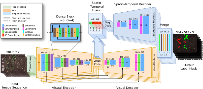
Figure 3: Architecture of our approach as described in Sec. III-A. Given a sequence of $S$ images, we first compute the visual code through the visual encoder. The visual code is then again upsampled with the visual decoder resulting in the visual features. The spatio-temporal fusion uses $S$ visual codes to encode the sequential context from multiple images resulting in the sequence code. Using the spatio-temporal decoder, we upsample the sequence code again resulting in the sequence features. Finally, the visual and sequence features are merged resulting in a pixel-wise label mask. In the figure, we included the size of the feature maps above the layers and the number of feature maps produced by each layer inside the layer. In the spatio-temporal fusion, we included the parameters $k$ and $d$ of the dilated convolution.

III-B Preprocessing

Preprocessing the input can help to improve the generalization capabilities of a classification system by aligning the training and test data distribution. The main goal of our preprocessing is to minimize the diversity of the inputs as much as possible in a data-driven way. We perform the preprocessing independently for each image and moreover separately on all channels, i.e. red, green, blue, and near infra-red. For each channel, we (i) remove noise by performing a blurring operation using a $[5\times 5]$ Gaussian kernel given by the standard normal distribution, i.e., $\mu=0$ and $\sigma^{2}=1$, (ii) standardize the data by the mean and standard deviation, and (iii) normalize and zero-center the values to the interval $[-1,1]$ as it is common practice for training FCNs. Fig. 4 illustrates the effect of our preprocessing for exemplary images captured with different sensor setups.

III-C Encoder-Decoder FCN

It has been shown that FCNs for semantic segmentation tasks achieve high performance for a large number of different applications [17, 18, 19, 25]. Commonly, FCN architectures follow the so-called “hourglass” structure referring to a downsampling of the resolution in the encoder followed by a complementary upsampling in the decoder to regain the full resolution of the input image for the pixel-wise segmentation. We design our network architecture keeping in mind that the classification needs to run in near real-time such that an actuator can directly act upon the incoming information. In addition to that we use a comparably small number of learnable parameters to obtain a model capacity which is sufficient for the three class prediction problem. Thus, we design a lightweight network for our task.

As a basic building block in our encoder-decoder FCN, we follow the so-called Fully Convolutional DenseNet (FC-DenseNet) [26], which combines the recently proposed densely connected CNNs organized as dense blocks [25] with fully convolutional networks (FCN) [16]. The key idea is a dense connectivity pattern which iteratively concatenates all computed feature maps of subsequent convolutional layers in a feed forward fashion. These “dense” connections encourage deeper layers to reuse features produced by earlier layers and additionally supports the gradient flow in the backward pass.

As commonly used in practice, we define our 2D convolutional layer as a composition of the following components: (1) 2D convolution, (2) rectified linear unit (ReLU) as non-linear activation, (3) batch normalization [15] and (4) dropout [27]. We repeatedly apply bottleneck layers to the feature volumes and thus keep the number of feature maps small while achieving a deep architecture. Our bottleneck is a 2D convolutional layer with a $[1\times 1]$ kernel.

A dense block is given by a stack of $L$ subsequent 2D convolutional layers operating on feature maps with the same spatial resolution. Fig. 3 depicts the information flow in a dense block. The input of the $l^{\text{th}}$ 2D convolutional layer is given by a concatenation of all feature maps produced by the previous layers, whereas the output feature volume is given by the concatenation of the newly computed feature maps within the dense block. Here, all the concatenations are performed along the feature axis. The number of the produced feature maps is called the growth rate $G$ of a dense block [25]. We consequently use $2G$ kernels for the bottleneck layers within a dense block to reduce the computational cost in the subsequent 2D convolutional layers.

Fig. 3 illustrates the information flow through the FCN. The first layer in the encoder is a 2D convolutional layer augmenting the 4-channel images using $32$ $[5\times 5]$ kernels. The following operations in the encoder are given by a recurring composition of dense blocks, bottleneck layers and downsampling operations, where we concatenate the input of a dense block with its output feature maps. We perform the downsampling by strided convolutions employing 2D convolutional layers with an $[5\times 5]$ kernel and a stride of $2$. All bottleneck layers between dense blocks compress the feature volumes by a learnable halving along the feature axis. In the decoder, we revert the downsampling by a strided transposed convolution [28] with a $[2\times 2]$ kernel and a stride of $2$. To facilitate the recovery of spatial information, we concatenate feature maps produced by the dense blocks in the encoder with the corresponding feature maps produced by the learnable upsampling and feed them into a bottleneck layers followed by a dense blocks. Contrary to the encoder, we reduce the expansion of the number of feature maps within the decoder by omitting the concatenation of a dense blocks input with its respective output.

III-D Sequential Module

To learn information about the crop and weed arrangement, the network needs to take the whole sequence corresponding to a crop row into account. The sequential module represents our key architectural design contribution to enable sequential data processing. It can be seen as an additional parallel pathway for the information flow and consists of three subsequent parts, i.e. the (i) spatio-temporal fusion, the (ii) spatio-temporal decoder and the (iii) merge layer.

The spatio-temporal fusion is the core part of the sequential processing. First, we create a sequential feature volume by concatenating all visual code volumes of the sequence along an additional time dimension. Second, we compute a spatio-temporal feature volume, the sequence code, as we process the built sequential feature volume by a stack of three 3D convolutional layers. We define the 3D convolutional layer analogous to the 2D convolutional layer, i.e. a composition of convolution, ReLu, batch normalization and dropout. In each 3D convolutional layer, we use $16$ 3D kernels with a size of $[5\times 5\times S]$ to allow the network to learn weight updates under consideration of the whole input sequence. We apply the batch normalization to all feature maps jointly regardless of their position in the sequence.

As a further architectural design choice, we increase the receptive field for subsequent applied 3D convolutional layers in their spatial domain. Thus, the network can potentially exploit more context information to extract the geometric arrangement pattern of the plants. To achieve this, we increased the kernel size $k$ and the dilation rate $d$ of the 3D kernels for subsequent 3D convolutional layers. More concretely, we increase $k$ and $d$ only for the spatial domain of the convolutional operation, i.e. $[k\times k\times S]$ with $k=\{5,7,9\}$ and $[d\times d\times 1]$ with $d=\{1,2,4\}$. This leads to a larger receptive field of the spatio-temporal fusion allowing the model to consider the whole encoded content of all images along the sequence. In our experiments, we show that the model gains performance by using an increasing receptive field within the spatio-temporal fusion.

The spatio-temporal decoder is the second part of the sequential module that upsamples the produced sequence code to the desired output resolution resulting in the sequence features. Analogous to the visual decoder, we recurrently perform the upsampling followed by a bottleneck layer and a dense block to generate a pixel-wise sequence features map. To achieve an independent data processing of the spatio-temporal decoder and visual decoder, we neither share weights between both pathways nor connect them via skip connections with the encoder of the FCN.

The last building block of the sequential module is the merge layer. Its main objectives are to merge the visual features with the sequence features and to compute the label mask as the output of the system. First, we concatenate the input feature volumes along their feature axis and pass the result to a bottleneck layer using $12$ kernels, where the actual merge takes place. Then we pass the resulting feature volume through a stack of two 2D convolutional layers. Finally, we convolve the feature volume into the label mask using a bottleneck layer with $3$ kernels for respective class labels and perform a pixel-wise softmax along the feature axis. Further details on the specific number of layers and parameters can be found in Fig. 3 and Sec. IV, where we also evaluate the influence of our key architectural design decisions.

IV Experimental Evaluation

Our experiments are designed to show the capabilities of our method and to support our key claims, which are: (i) Our approach generalizes well and robustly identifies the crops and weeds after the visual appearance of the plants and the soil has changed without the need for adapting the model through retraining and (ii) is able to extract features about the spatial arrangement of the plantation and is able to perform the crop-weed classification task solely using this geometric information source.

IV-A Experimental Setup

TABLE I: Dataset Information

	Bonn2016	Bonn2017	Stuttgart
# images	10,036	864	2,584
crop pixels	1.7%	0.3%	1.5%
approx. crop size	0.5-100 cm2	0.5-3 cm2	3-25 cm2
weed pixels	0.7%	0.05%	0.7%
approx. weed size	0.5-60 cm2	0.5-3 cm2	2-60 cm2

Bonn2016	Bonn2017	Stuttgart

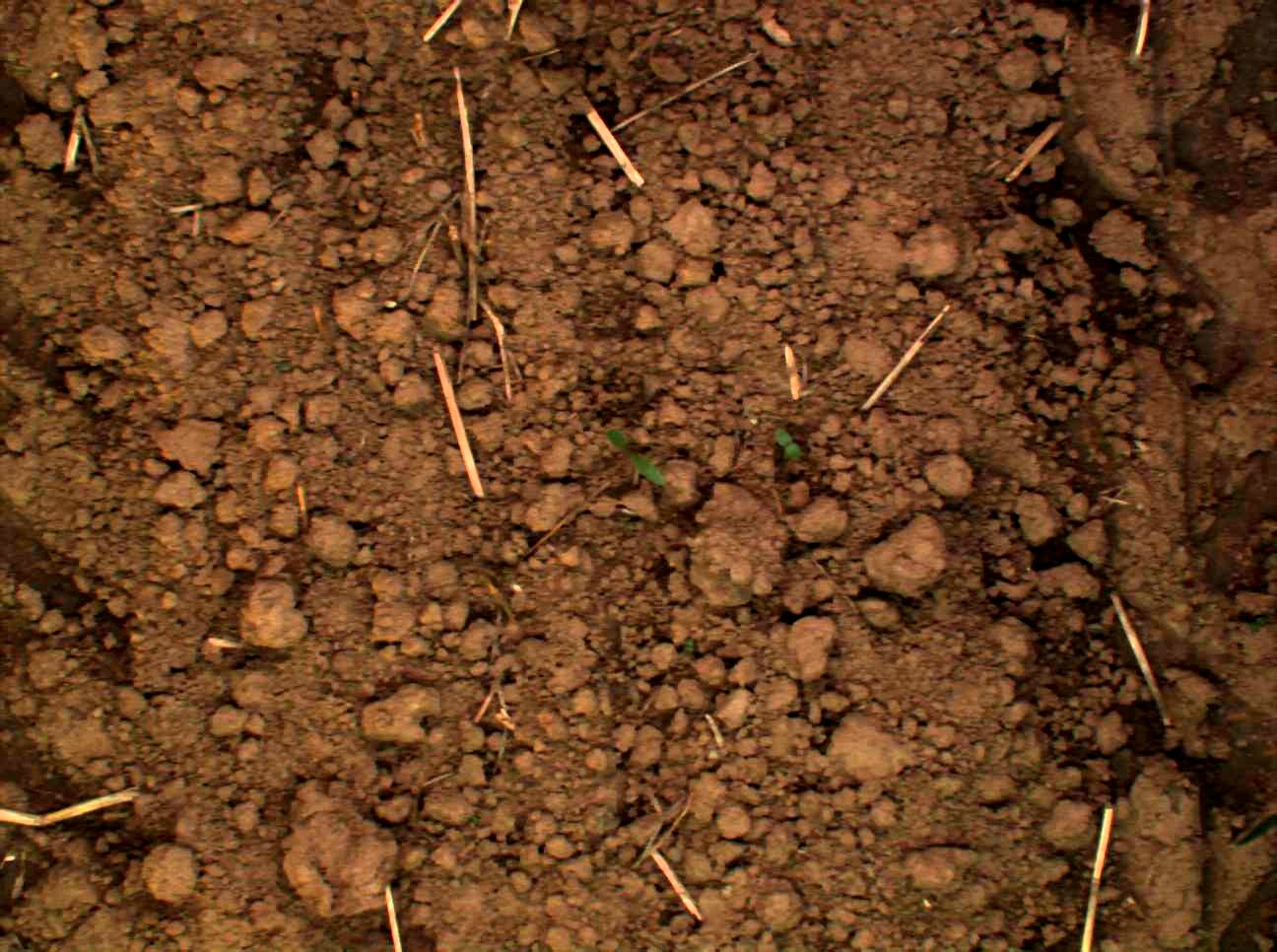
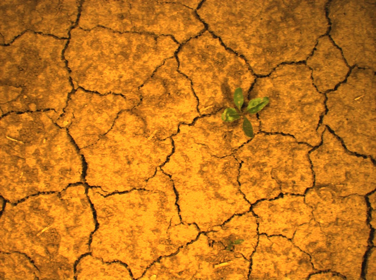
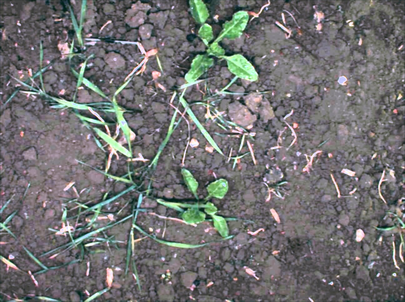
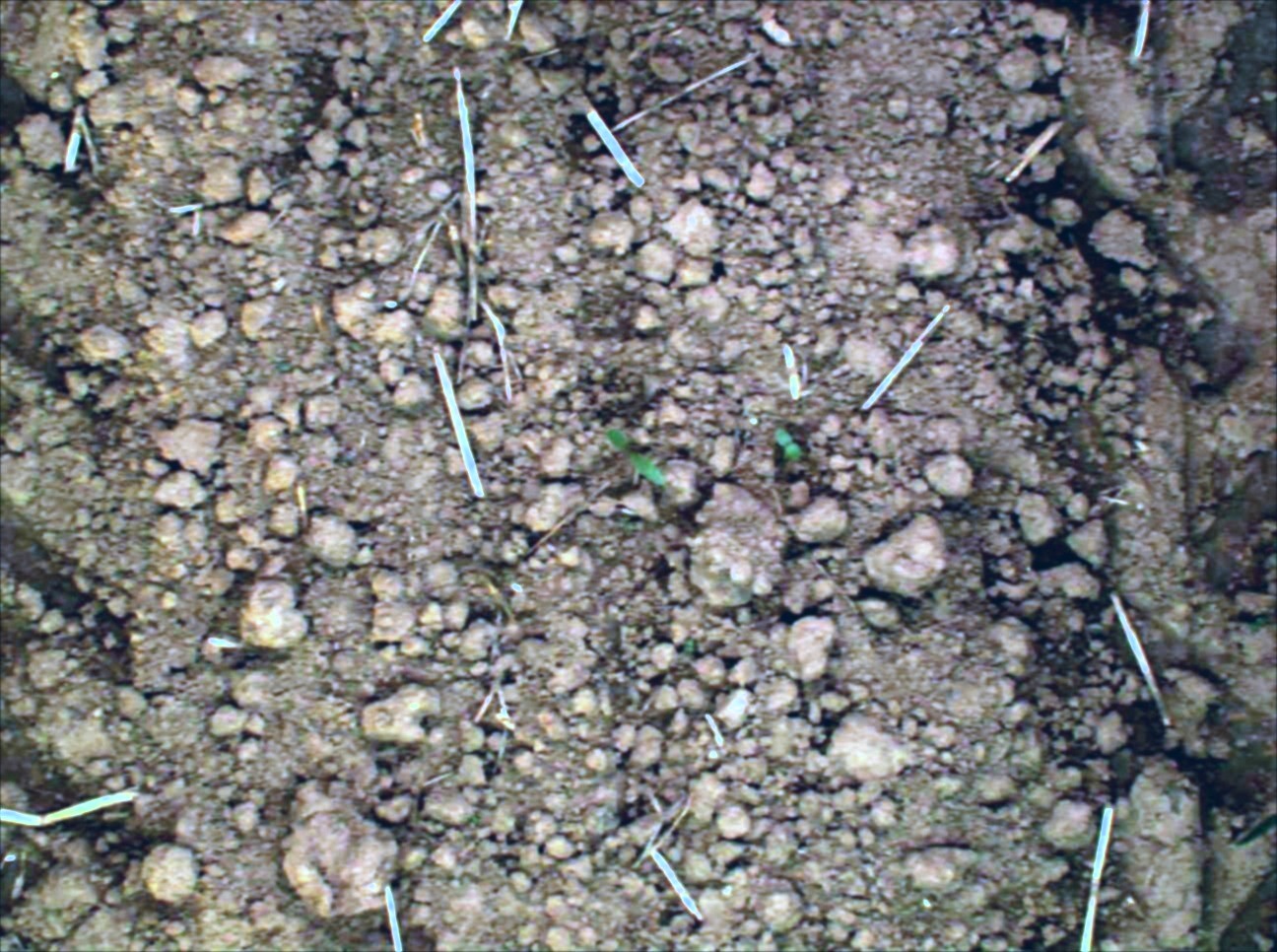
Figure 4: Top: RGB images from each dataset containing different crop growth stages, weed types, illumination conditions and soil types. Bottom: Example RGB images after preprocessing.

The experiments are conducted on different sugar beet fields located near Bonn and near Stuttgart in Germany. Each dataset has been recorded with different variants of the BOSCH DeepField Robotics BoniRob platform. All robots use the 4-channel RGB+NIR camera JAI AD-130 GE mounted in nadir view, but with different lighting setups. Every dataset contains crops of different growth stages, while the datasets differ from each other in terms of the weed and soil types. The dataset collected in Bonn is publicly available and contains data collected over two month on a sugar beet field. A detailed description of the data, the setup for its acquisition, and the robot is provided by Chebrolu et al.  [10].

We evaluate our system in terms of an object-wise performance, i.e. a metric for measuring the performance on plant-level. Here, we compare the predicted label mask with the crop and weed objects given by the class-wise connected components from the corresponding ground truth segments. We consider plant segments with a minimum size of $0.5$ cm² in object space and consider smaller objects to be noise as they are only represented by around 50 pixels and therefore would bias the performance. In all experiments, we only consider non-overlapping images to have separate training, validation, and test data.

We refer to the baseline approach as our encoder-decoder FCN using the proposed preprocessing but without the sequential module. We refer to our approach as the combination of the baseline with our proposed sequential module. Note that we use a comparable number of parameters for the baseline approach to exclude that the performance is affected by less capacity of the model.

For comparison, we also evaluate the performance on our recently published approaches: (i) using a semi-supervised vision and geometry based approach based on random forests [22] and (ii) employing a purely visual FCN classifier solely based on RGB data [5], which additionally takes vegetation indices as additional plant features (PF) into account. We refer to these approaches with RF and FCN+PF respectively.

IV-B Parameters

In our experiments, we train all networks from scratch using downsampled images with a resolution $W=512$ and $H=384$ which yields a ground resolution of around $1\,\frac{\text{mm}}{\text{pixel}}$. We use a sequence length $S=5$ and use a grow rate $G=4$ for the dense blocks. For training our architecture, we follow the common best practices: we initialize the weights as proposed by He et al.  [29] and use the RMSPROP optimizer with a mini-batch size of $B=2$ leading to $10$ images per mini-batch. We use a weighted cross- entropy loss, where we penalize prediction errors for the crops and weeds by a factor of $10$. We set the initial learning rate to $0.01$ and divide it by $10$ after $10$ and $25$ epochs respectively. We stop the training after $200$ epochs corresponding to a total duration of approx. $58$ hours. We use dropout with a rate of $\frac{1}{3}$. We implemented our approach using Tensorflow and it provides classification results with a processing rate of approximately $5\,$Hz ($200$ ms) on a NVIDIA Geforce GTX 1080 Ti GPU. We selected the values for $S$, $G$, $B$ and use RMSPROP with the proposed learning rate schedule as this combination performs best within our hyperparameter search on the Bonn2016 validation dataset. We choose $S=5$ as it is a good trade-off between the present spatial information and the computational cost per sequence.

IV-C Performance Under Changing Environmental Conditions

TABLE II: Cross-dataset performance (object-wise) when training on Bonn2016 and testing on Stuttgart

Approach	avg. F1 [%]	Recall [%]		Precision [%]
		Crop	Weed	Crop	Weed
our	92.4	95.4	87.8	89.1	97.9
baseline	81.9	75.2	80.0	87.7	85.9
RF [22]	48.0	36.4	66.5	34.7	55.4
FCN+PF [5]	74.2	85.1	65.2	64.6	87.9
RF⋆ [22]	91.8	95.1	92.2	85.2	95.4
FCN+PF⋆ [5]	90.5	91.4	89.1	86.6	95.5
$\star$ Approach with additional labeling effort and retraining of classifier.

The first experiment is designed to support the claim of superior generalization capabilities with a high performance of our approach, even when the training and test data notably differ concerning the visual appearance in the image data. Note that we do not perform retraining in this experiment as its main purpose is to represent practical challenges for a crop-weed classification, as argued by Slaughter et al.  [9]. We evaluate the performance in case that we operate with a different robotic system in previously unseen fields with changes in the visual appearance in the image data induced by different weed types and weed pressure and soil conditions. Therefore, we train the classification model on the entire data of the Bonn2016 dataset and evaluate the performance on the Stuttgart and Bonn2017 datasets. For a fair comparison with RF [22], we do not employ the online learning and provide no labeled data from the targeted field to initialize the random forest classifier.

TABLE III: Cross-dataset performance (object-wise) when training on Bonn2016 and testing on Bonn2017

Approach	avg. F1 [%]	Recall [%]		Precision [%]
		Crop	Weed	Crop	Weed
our	86.6	91.2	95.3	90.3	72.7
baseline	73.7	82.0	93.9	80.6	51.1
RF [22]	50.2	30.5	55.7	42.7	77.5
FCN+PF [5]	67.3	83.1	47.4	92.2	46.8
RF⋆ [22]	92.8	96.1	92.0	86.2	97.6
FCN+PF⋆ [5]	89.1	95.6	69.8	92.4	85.7
$\star$ Approach with additional labeling effort and retraining of classifier.

Tab. II summarizes the obtained performance on the Stuttgart dataset. Our approach outperforms all other methods. We detect more than $95\%$ of the crops and around $88\%$ of the weeds and gain around $10\%$ performance to the second best in terms of the average F1-score. The results obtained on the Bonn2017 dataset confirm this observation as we observe a margin of around $5\%$ to the second best approach with respect to the average F1-score. Tab. III shows the achieved performance for the Bonn2017 dataset. Here, our approach detects most of the plants correctly with a recall of $91\%$ of the crops and $95\%$ of the weeds.

Fig. 2 illustrates the performance our our approach on the Stuttgart dataset. Aside from the fact that we perform the classification in a sequence-to-one fashion, we present the predictions over the whole sequence. This result supports the high recall obtained for the crop class. Furthermore, it can be seen that the crops and weed pixels are precisely separated from the soil, which indicates a high performance for the vegetation separation.

The changes in the visual appearance of the image data of the Stuttgart and Bonn2017 datasets compared to the Bonn2016 training dataset lead to a substantial decrease of the obtained performance by the pure visual approaches, i.e., the baseline and FCN+PF [5]. The comparison suggests that the additional exploitation of the arrangement information leads to a better generalization to other field environments. The performance of the RF [22] breaks down due to a wrong initialization of the geometrical classifier induced by wrong prediction of the visual classifier in the first iteration. Note that we executed a t-test for our approach and the respective baselines in Tab. II and Tab. III. In all experiments, our approach was significantly better than the baselines under a 99% confidence level.

The two bottom rows of the tables reflect the obtained performance for the FCN+PF^⋆ [5] and RF^⋆ [22], when the classification models have access to small amounts of training data coming from the target field, e.g., to adapt their parameters to the data distribution through retraining. Therefore, we manually labeled $100$ additional images from the test dataset and used this data to retrain the FCN+PF^⋆ [5] and RF^⋆ [22] classifier. Our approach obtains a comparable performance terms of the average F1-score, i.e., above $90$ %, for the Stuttgart dataset. For the Bonn2017 dataset our approach cannot reach this level of performance. The results indicate that retraining of classification models leads to a more reliable performance, but with our approach we make a big step towards bridging this gap.

Thus, this experiment clearly shows the superior generalization capabilities of our approach and the impact of exploiting sequential data. However, we will further investigate the influence of the sequential module and other key design decision in our ablation study in Sec. IV-E.

IV-D Performance Under Changing Growth Stage

TABLE IV: Generalization capabilities: Test performance on data containing different growth stages of the sugar beets

Approach	avg. F1 [%]	Recall [%]		Precision [%]
		Crop	Weed	Crop	Weed
our	92.3	96.1	92.4	96.6	81.5
baseline	69.3	94.1	45.5	71.4	77.9

This experiment is designed to evaluate the generalization capabilities of our approach regarding changes due the growth stage. This scenario is typical in practical use cases, where the robot enters the same field again after some time. We evaluate this by choosing training and test subsets from the Bonn2016 datasets with a temporal difference of around $10$ days. The training data is given by around $1,500$ images acquired in early season at the two-leave growth stage with an average leaf of around $1$ cm². The test data is given by images from another location in the same field captured later in time, where the sugar beets have an average size of $6$ cm², i.e. about six times larger than the training examples.

Tab. IV shows the obtained performance of our approach in comparison to the baseline model. With an average F1-score of $91\%$, our approach provides a solid performance under changing growth stages. The results show that our approach can exploit the repetitive arrangement pattern of the sugar beets from the sequential data stream, since it better generalizes to other growth stages compared to the baseline model. The performance of the baseline model suffers from the different visual appearance as it solely relies on visual cues. The decrease in performance of the baseline model underlines that exploiting sequential information compensates for changes in the visual appearance.

IV-E Ablation Study

TABLE V: Ablation Study

	Approach	Bonn2016	Bonn2017	Stuttgart
	Vanilla FCN	96.7	72.5	69.3
+	Preprocessing	96.5	79.1	77.8
+	Sequential	97.5	83.0	89.2
+	Spatial Context (Our)	96.9	86.6	92.4
All classifiers are trained on the Bonn2016 training data.

In this experiment, we show the effect of the most central architectural design choices resulting in the largest gain and improvement of the generalization capability. Therefore, we evaluate different architectural configurations of our approach using 75% of the Bonn2016 dataset for training and evaluate the performance on (i) 20% held-out testset of Bonn2016, (ii) Stuttgart and (iii) Bonn2017.

Tab. V reports the obtained object-wise test performance with respect to the average F1-score. Here, we start with a vanilla FCN corresponding to our Encoder-Decoder FCN described in Sec. III-C. Then, we add our proposed preprocessing which helps to generalize to different fields. It minimizes the effect of different lighting conditions (see Fig. 4) at the cost of a neglectable decrease in performance on the Bonn2016 dataset. We can furthermore improve the generalization capabilities by using the sequential module on top. Adding then more spatial context by increasing the receptive field of the sequential module by using bigger kernels and dilated convolutions further improves the performance.

The high performance of all configurations on the held-out Bonn2016 data indicates that FCNs generally obtain a stable and high performance under a comparably low diversity in the data distribution. Thus, diversity between the training and test data is crucial to evaluate crop-weed classification system under practical circumstances. We conclude that preprocessing and exploitation of the repetitive pattern given by the crop arrangement helps to improve the generalization capabilities of our sequential FCN-based crop-weed classification system.

IV-F Experiment on Learning the Crop-Weed Arrangement

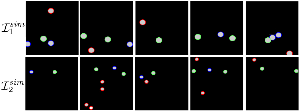
Figure 5: Two realizations of simulated image sequences $\mathcal{I}^{\mathit{sim}}_{1}$ and $\mathcal{I}^{\mathit{sim}}_{2}$ with different properties as mentioned in Sec. IV-F. The blob size is uniform within a sequence. The colored contours refer to the corresponding ground truth labels, i.e. crop (green), weed (red) and intra-row weed (blue).

Using experiments with simulated data, we finally demonstrate the capability of our approach to extract information about the spatial arrangement of the crops and weeds. For this purpose, we create input data providing solely the signal of the plant arrangement as a potential information to distinguish the crop and weeds.

We render binary image sequences encoding the crops and weeds as uniform sized blobs while imitating (i) the crop-weed arrangement and (ii) the acquisition setup of the robotic system in terms of the camera setup and its motion in space. Fig. 5 depicts two simulated sequences and their corresponding ground truth information. Note that within a sequence, we only model blobs of uniform size. Thus, we provide neither spectral nor shape information as a potential input signal for the classification task. We hypothesize that an algorithm solving the classification task given the simulated data is also able to learn features describing the arrangement of crops and weeds.

We furthermore explicitly simulate intra-row weeds, i.e., weeds located close to the crop row. To properly detect intra-row weeds, the classifier needs to learn the intra-row distance between crops instead of solely memorizing that all vegetation growing close to the center line of a crop row belongs to the crop class. We model the following properties for creating the simulated sequences, as shown in Fig. 5: (1) intra-row distance ($15$-$25$ cm), (2) inter-row distance ($30$-$60$ cm), (3) weed pressure ($0$-$200$% w.r.t. the crops present in the sequence), (4) plant size ($0.5$-$8.0$ cm²), and (5) the camera motion along the row by a slight variation of the steering angle. We pertubate the plant locations by Gaussian noise ($\mu=0$ and $\sigma^{2}=10\%$ of the intra-row distance).

TABLE VI: Test performance on simulated data

Approach	avg.	Recall [%]			Precision [%]
	F1 [%]	Crop	Weed	Intra-Weed	Crop	Weed	Intra-Weed
our	93.6	95.4	99.1	84.2	98.3	99.1	85.5
baseline	47.3	61.1	59.3	9.4	75.9	80.4	4.4

Tab. VI shows the performance of our approach compared to the baseline approach. These results demonstrate that our approach can exploit the sequential information to extract the pattern of the crop arrangement for the classification task. In contrast, the baseline model is unable to properly identify the crops and weeds due to missing shape information.

V Conclusion

In this paper, we presented a novel approach for precision agriculture robots that provides a pixel-wise semantic segmentation into crop and weed. It exploits a fully convolutional network integrating sequential information. We proposed to encode the spatial arrangement of plants in a row using 3D convolutions over an image sequence. Our thorough experimental evaluation using real-world data demonstrates that our system (i) generalizes better to unseen fields in comparison to other state-of-the-art approaches and (ii) is able to robustly classify crop in different growth stages. Finally, we show that the proposed sequential module actually encodes the spatial arrangement of the plants through simulation.

References

- [1] M. Müter, P. S. Lammers, and L. Damerow, “Development of an intra-row weeding system using electric servo drives and machine vision for plant detection,” in Proc. of the International Conf. on Agricultural Engineering LAND.TECHNIK (AgEng), 2013.
- [2] F. Langsenkamp, F. Sellmann, M. Kohlbrecher, A. Kielhorn, W. Strothmann, A. Michaels, A. Ruckelshausen, and D. Trautz, “Tube stamp for mechanical intra-row individual plant weed control,” in Proc. of the International Conf. of Agricultural Engineering (CIGR), 09 2014.
- [3] S. Haug, A. Michaels, P. Biber, and J. Ostermann, “Plant Classification System for Crop / Weed Discrimination without Segmentation,” in Proc. of the IEEE Winter Conf. on Applications of Computer Vision (WACV), 2014.
- [4] P. Lottes, R. Khanna, J. Pfeifer, R. Siegwart, and C. Stachniss, “UAV-Based Crop and Weed Classification for Smart Farming,” in Proc. of the IEEE Intl. Conf. on Robotics & Automation (ICRA), 2017.
- [5] A. Milioto, P. Lottes, and C. Stachniss, “Real-time Semantic Segmentation of Crop and Weed for Precision Agriculture Robots Leveraging Background Knowledge in CNNs,” in Proc. of the IEEE Intl. Conf. on Robotics & Automation (ICRA), 2018.
- [6] A. K. Mortensen, M. Dyrmann, H. Karstoft, R. N. Jörgensen, and R. Gislum, “Semantic Segmentation of Mixed Crops using Deep Convolutional Neural Network,” in Proc. of the International Conf. of Agricultural Engineering (CIGR), 2016.
- [7] A. Nieuwenhuizen, “Automated detection and control of volunteer potato plants,” Ph.D. dissertation, Wageningen University, 2009.
- [8] C. Potena, D. Nardi, and A. Pretto, “Fast and accurate crop and weed identification with summarized train sets for precision agriculture,” in Proc. of Int. Conf. on Intelligent Autonomous Systems (IAS), 2016.
- [9] D. Slaughter, D. Giles, and D. Downey, “Autonomous robotic weed control systems: A review,” Computers and Electronics in Agriculture, vol. 61, no. 1, pp. 63 – 78, 2008.
- [10] N. Chebrolu, P. Lottes, A. Schaefer, W. Winterhalter, W. Burgard, and C. Stachniss, “Agricultural Robot Dataset for Plant Classification, Localization and Mapping on Sugar Beet Fields,” Intl. Journal of Robotics Research (IJRR), 2017.
- [11] P. Lottes, M. Hoeferlin, S. Sanders, and C. Stachniss, “Effective Vision-Based Classification for Separating Sugar Beets and Weeds for Precision Farming,” Journal of Field Robotics (JFR), 2016.
- [12] M. Cicco, C. Potena, G. Grisetti, and A. Pretto, “Automatic Model Based Dataset Generation for Fast and Accurate Crop and Weeds Detection,” in Proc. of the IEEE/RSJ Intl. Conf. on Intelligent Robots and Systems (IROS), 2017.
- [13] C. McCool, T. Perez, and B. Upcroft, “Mixtures of Lightweight Deep Convolutional Neural Networks: Applied to Agricultural Robotics,” IEEE Robotics and Automation Letters (RA-L), 2017.
- [14] A. Milioto, P. Lottes, and C. Stachniss, “Real-time Blob-wise Sugar Beets vs Weeds Classification for Monitoring Fields using Convolutional Neural Networks,” in Proc. of the Intl. Conf. on Unmanned Aerial Vehicles in Geomatics, 2017.
- [15] C. Szegedy, V. Vanhoucke, S. Ioffe, J. Shlens, and Z. Wojna, “Rethinking the Inception Architecture for Computer Vision,” in Proc. of the IEEE Conf. on Computer Vision and Pattern Recognition (CVPR), 2016.
- [16] J. Long, E. Shelhamer, and T. Darrell, “Fully Convolutional Networks for Semantic Segmentation,” in Proc. of the IEEE Conf. on Computer Vision and Pattern Recognition (CVPR), 2015.
- [17] V. Badrinarayanan, A. Kendall, and R. Cipolla, “SegNet: A Deep Convolutional Encoder-Decoder Architecture for Image Segmentation,” IEEE Trans. on Pattern Analalysis and Machine Intelligence (TPAMI), vol. 39, no. 12, pp. 2481–2495, 2017.
- [18] A. Paszke, A. Chaurasia, S. Kim, and E. Culurciello, “ENet: Deep Neural Network Architecture for Real-Time Semantic Segmentation,” arXiv preprint, vol. abs/1606.02147, 2016.
- [19] O. Ronneberger, P.Fischer, and T. Brox, “U-Net: Convolutional Networks for Biomedical Image Segmentation,” in Medical Image Computing and Computer-Assisted Intervention, ser. LNCS, vol. 9351. Springer, 2015, pp. 234–241.
- [20] I. Sa, Z. Chen, M. Popvic, R. Khanna, F. Liebisch, J. Nieto, and R. Siegwart, “weedNet: Dense Semantic Weed Classification Using Multispectral Images and MAV for Smart Farming,” IEEE Robotics and Automation Letters (RA-L), vol. 3, no. 1, pp. 588–595, 2018.
- [21] A. Wendel and J. Underwood, “Self-Supervised Weed Detection in Vegetable Crops Using Ground Based Hyperspectral Imaging,” in Proc. of the IEEE Intl. Conf. on Robotics & Automation (ICRA), 2016.
- [22] P. Lottes and C. Stachniss, “Semi-supervised online visual crop and weed classification in precision farming exploiting plant arrangement,” in Proc. of the IEEE/RSJ Intl. Conf. on Intelligent Robots and Systems (IROS), 2017.
- [23] D. Hall, F. Dayoub, T. Perez, and C. McCool, “A Transplantable System for Weed Classification by Agricultural Robotics,” in Proc. of the IEEE/RSJ Intl. Conf. on Intelligent Robots and Systems (IROS), 2017.
- [24] D. Hall, F. Dayoub, J. Kulk, and C. McCool, “Towards Unsupervised Weed Scouting for Agricultural Robotics,” in Proc. of the IEEE Intl. Conf. on Robotics & Automation (ICRA), 2017.
- [25] G. Huang, Z. Liu, L. v. d. Maaten, and K. Q. Weinberger, “Densely Connected Convolutional Networks,” in Proc. of the IEEE Conf. on Computer Vision and Pattern Recognition (CVPR), 2017.
- [26] S. Jégou, M. Drozdzal, D. Vázquez, A. Romero, and Y. Bengio, “The One Hundred Layers Tiramisu: Fully Convolutional DenseNets for Semantic Segmentation,” arXiv preprint:1611.09326, 2017.
- [27] N. Srivastava, G. Hinton, A. Krizhevsky, I. Sutskever, and R. Salakhutdinov, “Dropout: A Simple Way to Prevent Neural Networks from Overfitting,” Journal of Machine Learning Research (JMLR), vol. 15, pp. 1929–1958, 2014.
- [28] V. Dumoulin and F. Visin, “A guide to convolution arithmetic for deep learning,” arXiv preprint, 2018.
- [29] K. He, X. Zhang, S. Ren, and J. Sun, “Delving deep into rectifiers: Surpassing human-level performance on imagenet classification,” in Proc. of the IEEE Intl. Conf. on Computer Vision (ICCV), 2015.