Phase transitions in a multistate majority-vote model on complex networks

Abstract

We generalize the original majority-vote (MV) model from two states to arbitrary $p$ states and study the order-disorder phase transitions in such a $p$-state MV model on complex networks. By extensive Monte Carlo simulations and a mean-field theory, we show that for $p\geq 3$ the order of phase transition is essentially different from a continuous second-order phase transition in the original two-state MV model. Instead, for $p\geq 3$ the model displays a discontinuous first-order phase transition, which is manifested by the appearance of the hysteresis phenomenon near the phase transition. Within the hysteresis loop, the ordered phase and disordered phase are coexisting and rare flips between the two phases can be observed due to the finite-size fluctuation. Moreover, we investigate the type of phase transition under a slightly modified dynamics [Melo et al. J. Stat. Mech. P11032 (2010)]. We find that the order of phase transition in the three-state MV model depends on the degree heterogeneity of networks. For $p\geq 4$, both dynamics produce the first-order phase transitions.

I Introduction

Spin models such as the Ising model play fundamental roles in studying phase transitions and critical phenomena in the field of statistical physics Baxter (1989). They have also significant implications for understanding various social and biological phenomena where co-ordination dynamics is observed, e.g., in consensus formation and adoption of innovations Stauffer (2008); Dorogovtsev et al. (2008); Castellano et al. (2009). The spin orientations can represent the choices made by an agent on the basis of information about its local neighborhood. Along these lines, so much has been done in recent years in social systems from human cooperation Perc et al. (2017); Perc (2016) to vaccination Wang et al. (2016); Pastor-Satorras et al. (2015) to crime D’Orsogna and Perc (2015) and saving human lives Helbing et al. (2015), as well as biological systems from collective motion Vicsek and Zafeiris (2012) to transport phenomena Chou et al. (2011) to criticality and dynamical scaling Muñoz (2017).

The majority-vote (MV) model is one of the simplest nonequilibrium generalizations of the Ising model de Oliveira (1992). In the model, each spin is assigned to a binary variable. At each time step, each spin tends to align with the local neighborhood majority but with a noise intensity $f$ giving the probability of misalignment. The MV model not only plays an important role in the study of nonequilibrium phase transitions, but it also help to understand opinion dynamics in social systems Castellano et al. (2009). The two-state MV model has been extensively studied in various interacting substrates, such as regular lattices Kwak et al. (2007); Wu and Holme (2010); Acuña Lara et al. (2014); Acuña Lara and Sastre (2012); Yu (2017), random graphs Pereira and Moreira (2005); Lima et al. (2008), small-world networks Campos et al. (2003); Luz and Lima (2007); Stone and McKay (2015), scale-free networks Lima (2006); Lima and Malarz (2006); Chen et al. (2015), modular networks Huang et al. (2015), complete graphs Fronczak and Fronczak (2017), and spatially embedded networks Sampaio Filho et al. (2016). With the exception of an inertial effect that was considered Chen et al. (2017a, b); Harunari et al. (2017), all the previous studies have shown that the two-state MV model presents a continuous second-order phase transition at a critical value of $f$.

The multistate MV model is a natural generalization of the two-state case, As its equilibrium counterpart, the Potts model is a generalization of the Ising model Wu (1982). The three-state MV model on a regular lattice was considered in Brunstein and Tomé (1999); Tomé and Petri (2002), where the authors found that the critical exponents for this non-equilibrium model are in agreement with the ones for the equilibrium three-state Potts model, supporting the conjecture of Grinstein et al. (1985). Melo et al. studied the three-state MV model on random graphs and showed that the phase transition is continuous and the critical noise is an increasing function of the mean connectivity of the graph Melo et al. (2010). Li et al. studied a three-state MV model with a slightly different dynamics in an annealed random network, and they showed the phase transition belongs to a first-order type Li et al. (2016). Lima introduced an unoccupied state to the two-state MV model in square lattices and found that this model also falls into the Ising universality Lima (2012). Costa et al. generalized the state variable of the MV model from a discrete case to a continuous one, and found that a Kosterlitz-Thouless-like phase appears in low values of noise Costa and de Souza (2005).

In the present work, we generalize the MV model to arbitrary multiple states, and we focus on the natures of phase transitions in the multi-state MV model on complex networks. By Monte Carlo (MC) simulation, we show that if the number of states is greater than or equal to 3, a clear hysteresis loop is observed as noise is dialed up and down, which is a typical feature of a first-order phase transition. Moreover, we propose a mean-field theory to validate the simulation results. Finally, we investigate the type of phase transition under a slightly modified dynamics Brunstein and Tomé (1999); Tomé and Petri (2002); Melo et al. (2010). We find that such a small difference in dynamics leads to the essential difference in the type of phase transition in the three-state MV model on Erdös-Rényi (ER) random networks or higher degree heterogeneous networks.

II Model

We generalize the original MV model from two states to arbitrary multiple states. The model is defined on an unweighted network with size $N$ described by an $N\times N$ adjacency matrix, whose elements $A_{ij}=1$ if a directed edge is emanated from node $j$ and ended at node $i$, and $A_{ij}=0$ otherwise. Each node $i$ can be in any of the $p$ states: ${\sigma_{i}}\in\{1,\cdots,p\}$. The number of the neighbors of node $i$ in each state $\alpha$ can be calculated as ${n_{i}^{\alpha}}=\sum\nolimits_{j=1}^{N}A_{ji}{\delta(\sigma_{j}-\alpha)}$, where $\delta(x)$ is the Kronecker symbol defined as $\delta=1$ if $x=0$ and $\delta=0$ otherwise.

In the following, we introduce two slightly different types of dynamical rules. For both dynamics, the node $i$ take the same value as the majority spin with the probability $1-f$, i.e., ${\sigma_{i}}={\left.\alpha\right|_{{n_{i}^{\alpha}}=\max\{{n_{i}^{1}},\cdots,{n_{i}^{q}}\}}}$. With the supplementary probability $f$, the node $i$ takes the same value as the minority spin, i.e., ${\sigma_{i}}={\left.\alpha\right|_{{n_{i}^{\alpha}}=\min\{{n_{i}^{1}},\cdots,{n_{i}^{q}}\}}}$ for type-I dynamics. For type-II dynamics, the node $i$ takes the same value as that of nonmajority spins (not necessarily the minority spin), i.e., ${\sigma_{i}}={\left.\alpha\right|_{{n_{i}^{\alpha}}\neq\max\{{n_{i}^{1}},\cdots,{n_{i}^{q}}\}}}$. If more than one candidate state is in the majority spin or in the minority spin, we randomly choose one of them. Here, the probability $f$ is called the noise intensity, which plays a similar role to the temperature in equilibrium systems and measures the probability of disagreeing with the majority of neighbors. For convenience, the former and the latter are called the type-I and type-II $p$-state MV model, respectively. If $p=2$, both dynamics are mutually equivalent and recover to the original two-state MV model. We should note that the type-II three-state MV model shows continuous phase transitions on square lattices Brunstein and Tomé (1999); Tomé and Petri (2002) and ER random networks Melo et al. (2010).

To characterize the critical behavior of the model, we define the order parameter as the modulus of the magnetization vector, that is, $m={\left({\sum\nolimits_{\alpha=1}^{p}{m_{\alpha}^{2}}}\right)^{1/2}}$, whose components are given by

$${m_{\alpha}}=\sqrt{\frac{p}{{p-1}}}\left[{\frac{1}{N}\sum\limits_{i}{\delta\left({\alpha-{\sigma_{i}}}\right)-\frac{1}{p}}}\right],$$ (1)

where the factor $\sqrt{p/(p-1)}$ is used to normalize the magnetization vector.

III Results

III.1 Type-I dynamics

We first focus on the type-I three-state MV model. By performing extensive MC simulations on ER random networks Erdös and Rényi (1960), we show the magnetization $m$ as a function of the noise intensity $f$, as shown in Fig. 1. The network size $N$ varies from Fig. 1(a) to Fig. 1(d): $N=10^{4}$ (a), $N=5\times 10^{4}$ (b), $N=10^{5}$ (c), and $N=5\times 10^{5}$ (d). The average degree $\left\langle k\right\rangle=10$ is kept unchanged. The simulation results are obtained by performing forward and backward simulations, respectively. The former is done by calculating the stationary value of $m$ as $f$ increases from 0.32 to 0.36 in steps of 0.001 and using the final configuration of the last simulation run as the initial condition of the next run, while the latter is performed by decreasing $f$ from 0.36 to 0.32 with the same step. One can see that as $f$ increases, $m$ abruptly jumps from nonzero to zero at $f=f_{cF}$, which shows that a sharp transition takes place for the order-disorder transition. Additionally, the curve corresponding to the backward simulations also shows a sharp transition from the disordered phase to the ordered phase at $f=f_{cB}$. These two sharp transitions occur at two different values of $f$, leading to a hysteresis loop with respect to the dependence of $m$ on $f$. The hysteresis loop becomes clearer as the network size increases. Such a feature indicates that a discontinuous first-order phase transition occurs in the type-I three-state MV model. This is in contrast to the original two-state MV model in which a continuous second-order phase transition was observed Pereira and Moreira (2005); Lima et al. (2008); Chen et al. (2015).

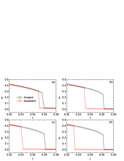
Figure 1: (Color online). First-order phase transition in the type-I three-state MV model on ER networks, characterized by a hysteresis loop of $m$ as noise intensity $f$ is dialed up and down. From (a)-(d), the network sizes are $N=10^{4}$, $5\times 10^{4}$, $10^{5}$, and $5\times 10^{5}$, respectively. The average degree is fixed at $\left\langle k\right\rangle=10$. Squares ($\Box$) and crosses ($\times$) correspond to forward and backward simulations, respectively.

To further verify the first-order nature of phase transition in the type-I three-state MV model, in Fig. 2(a-c) we show three long time series of $m$ corresponding to three distinct $f$ on an ER network with $N=10^{4}$ and $\left\langle k\right\rangle=10$. Here the noise intensity $f$ is chosen from the hysteresis region. One can see that in the hysteresis region the ordered and disordered phases are coexisting. Due the finite-size fluctuation, phase flipping between the ordered phase and the disordered phase can be rarely observed. As $f$ increases, the system spends more time on the disordered phase. In Fig. 2(d-f), we show the corresponding histograms for the distribution of $m$ at the three distinct $f$ as in Fig. 2(a-c). All the distributions are bimodal with a peak around $m=0$ and the other one at $m>0$. On the other hand, with the increase of $f$ the peak around $m=0$ becomes higher, indicating that the disordered phase becomes more stable with $f$. In general, as $N$ increases the fluctuation level becomes less significant and the mean time of phase switching increases exponentially with $N$, so that it is difficult to observe the phase flipping in the allowable computational time for larger $N$.

Figure 2: Coexistence of ordered and disordered phases in the hysteresis region for the type-I three-state MV model. Three typical time series of the magnetization $m$ on an ER network, corresponding to three different noise intensities chosen from the hysteresis region: $f=0.3472$ (a), $f=0.3475$ (b), and $f=0.3480$ (c). (d)-(f) show the corresponding histograms for the distribution of $m$ at the three values of $f$ as in (a-c), respectively. The networks parameters are $N=10^{4}$ and $\left\langle k\right\rangle=10$.

In Chen et al. (2015), we developed a heterogeneous mean-field theory to deal with the two-state MV model on degree uncorrelated networks, and we derived that the critical noise is determined by the ratio of the first-order moment to the 3/2-order moment of degree distribution. Also for the two-state MV model, a quenched mean-field theory was proposed recently Huang et al. (2017), which showed that the critical noise is determined by the largest eigenvalue of a deformed network adjacency matrix. In Li et al. (2016), we proposed a simple mean-field theory for the three-state MV model on a degree-regular random network in which each node is randomly connected to exactly $k$ neighbors, and degree distribution follows the $\delta$-function. In the following, we shall develop a heterogeneous mean-field theory that is applicable not only for any number $p$ of the states, but also for any degree distribution without degree-degree correlation.

To this end, let $x_{k}^{\alpha}$ denote the probability of nodes of degree $k$ being in the state $\alpha$. The dynamical equation for $x_{k}^{\alpha}$ reads,

$${\dot{x}_{k}^{\alpha}}=\sum\limits_{\beta\neq\alpha}{{x_{k}^{\beta}}}{w_{k}^{\beta\to\alpha}}-{x_{k}^{\alpha}}\sum\limits_{\beta\neq\alpha}{{w_{k}^{\alpha\to\beta}}},$$ (2)

where $w_{k}^{\alpha\to\beta}$ is the transition probability of nodes of degree $k$ from the state $\alpha$ to the state $\beta$. According to the definition of the MV model, the probability $w_{k}^{\alpha\to\beta}$ can be written as the sum of two parts,

$${w_{k}^{\alpha\to\beta}}=(1-f){P_{k}^{\beta}}+f{{\tilde{P}}_{k}^{\beta}},$$ (3)

where the first part is given by the probability $1-f$ of nodes of degree $k$ taking the majority-rule, multiplied by the probability $P_{k}^{\beta}$ that the state $\beta$ is the majority state among the neighbors of nodes of degree $k$. Likewise, the second part is the product of the probability $f$ of nodes of degree $k$ taking the minority-rule and the probability $\tilde{P}_{k}^{\beta}$ that the state $\beta$ is the minority state. Utilizing the normalization conditions, $\sum\nolimits_{\beta}{{x_{k}^{\beta}}}=\sum\nolimits_{\beta}{{P_{k}^{\beta}}}=\sum\nolimits_{\beta}{{{\tilde{P}}_{k}^{\beta}}}=1$, Eq. (2) can be simplified to

$${{\dot{x}}_{k}^{\alpha}}=-{x_{k}^{\alpha}}+(1-f){{P}_{k}^{\alpha}}+f{{\tilde{P}}_{k}^{\alpha}}.$$ (4)

In the steady state, $\dot{x}_{k}^{\alpha}=0$, we have

$${x_{k}^{\alpha}}=(1-f){P_{k}^{\alpha}}+f{{\tilde{P}}_{k}^{\alpha}}.$$ (5)

Let us further define $X_{\alpha}$ as the probability that for any node in the network, a randomly chosen nearest-neighbor node is in the state $\alpha$. For degree uncorrelated networks, the probability that a randomly chosen neighboring node has degree $k$ is $kP(k)/\left\langle k\right\rangle$ Dorogovtsev et al. (2008), where $P(k)$ is degree distribution defined as the probability that a node chosen at random has degree $k$ and $\left\langle k\right\rangle=\sum\nolimits_{k}{kP(k)}$ is the average degree. Therefore, The probabilities $x_{k}^{\alpha}$ and $X_{\alpha}$ satisfy the relation

$${X_{\alpha}}=\sum\limits_{k}{\frac{{kP(k)}}{{\left\langle k\right\rangle}}}x_{k}^{\alpha}.$$ (6)

Let $n_{\alpha}$ denote the number of neighbors of a node of degree $k$ in the state $\alpha$, and the probability of a given configuration $\{n_{\alpha}\}$ can be expressed as a multinominal distribution,

$${\Xi^{k}_{{n_{1}},\ldots,{n_{p}}}}\left({{X_{1}},\ldots,{X_{p}}}\right)=\frac{{k!}}{{\prod\limits_{\alpha}{{n_{\alpha}}!}}}\prod\limits_{\alpha}{X_{\alpha}^{{n_{\alpha}}}},$$ (7)

where $k=\sum\nolimits_{\alpha}n_{\alpha}$. Therefore, $P_{k}^{\alpha}$ and $\tilde{P}_{k}^{\alpha}$ can be written as

$$P_{k}^{\alpha}=\sum\limits_{\left.{\left\{{n_{\alpha}}\right\}}\right|n_{\alpha}\geq n_{\beta},\forall\beta\neq\alpha}{\frac{1}{{1+\Omega_{\alpha}\left({\left\{{n_{\alpha}}\right\}}\right)}}\Xi^{k}_{{n_{1}},\ldots,{n_{p}}}},$$ (8)

and

$$\tilde{P}_{k}^{\alpha}=\sum\limits_{\left.{\left\{{n_{\alpha}}\right\}}\right|n_{\alpha}\leq n_{\beta},\forall\beta\neq\alpha}{\frac{1}{{1+\Omega_{\alpha}\left({\left\{{n_{\alpha}}\right\}}\right)}}\Xi^{k}_{{n_{1}},\ldots,{n_{p}}}},$$ (9)

where $\Omega_{\alpha}\left({\left\{{n_{\alpha}}\right\}}\right)=\sum\nolimits_{\beta\neq\alpha}{\delta\left({{n_{\beta}}-{n_{\alpha}}}\right)}$ is the number of states whose number of nodes is the same as $n_{\alpha}$. If $\Omega_{\alpha}=0$, the state $\alpha$ is the only majority (minority) state, such that the factor $1/(1+\Omega_{\alpha})$ in Eq. (8) (Eq. (9)) equals to one. If $\Omega_{\alpha}=1$, there are two candidate majority (minority) states, such that the factor is equal to $1/2$, and so forth.

Substituting Eq. (5) into Eq. (6), we arrive at a set of self-consistent equations of $X_{\alpha}$,

$${X_{\alpha}}=(1-f)\sum\limits_{k}{\frac{{kP(k)}}{{\left\langle k\right\rangle}}}P_{k}^{\alpha}+f\sum\limits_{k}{\frac{{kP(k)}}{{\left\langle k\right\rangle}}}\tilde{P}_{k}^{\alpha}.$$ (10)

Notice that $X_{\alpha}=1/p$ is always a set of solutions of Eq. (10) since $P_{k}^{\alpha}=\tilde{P}_{k}^{\alpha}=1/p$ at $X_{\alpha}=1/p$. Such a trivial solution corresponds to the disordered phase ($m=0$). For convenience, the trivial solution is denoted by a vector $\textbf{X}=\textbf{X}^{*}\equiv(1/p,\cdots,1/p)^{\top}$, where the superscript $\top$ denotes the transpose. To evaluate the stability of $\textbf{X}^{*}$, we need to write down the Jacobian matrix J of Eq. (10). Since $X_{\alpha}$ satisfies the normalization condition $\sum\nolimits_{\alpha}{X^{\alpha}}=1$, only $p-1$ variables among $X_{\alpha}$ ($\alpha=1,\cdots,p$) are independent of each other. To the end, we select $X_{1},\cdots,X_{p-1}$ as the independent variables and therefore J is a $(p-1)$ dimensional square. The matrix elements of J are given by

$${J_{\alpha\beta}}=\left({1-f}\right)\sum\limits_{k}{\frac{{kP(k)}}{{\left\langle k\right\rangle}}}{\left.{\frac{{\partial P_{k}^{\alpha}}}{{\partial{X_{\beta}}}}}\right|_{{\textbf{X}^{*}}}}+f\sum\limits_{k}{\frac{{kP(k)}}{{\left\langle k\right\rangle}}}{\left.{\frac{{\partial\tilde{P}_{k}^{\alpha}}}{{\partial{X_{\beta}}}}}\right|_{{\textbf{X}^{*}}}},$$

(11)

with $\alpha,\beta=1,\cdots,p-1$. According to Eq. (8) and Eq. (9), we have

$${\left.{\frac{{\partial P_{k}^{\alpha}}}{{\partial{X_{\beta}}}}}\right|_{{\textbf{X}^{*}}}}=\sum\limits_{\left.{\left\{{{n_{\alpha}}}\right\}}\right|{n_{\alpha}}\geq{n_{\beta}},\forall\beta\neq\alpha}{\frac{1}{{1+{\Omega_{\alpha}}\left({\left\{{{n_{\alpha}}}\right\}}\right)}}}{\left.{\frac{{\partial\Xi_{{n_{1}},\ldots,{n_{p}}}^{k}}}{{\partial{X_{\beta}}}}}\right|_{{\textbf{X}^{*}}}},$$

(12)

and

$${\left.{\frac{{\partial\tilde{P}_{k}^{\alpha}}}{{\partial{X_{\beta}}}}}\right|_{{\textbf{X}^{*}}}}=\sum\limits_{\left.{\left\{{{n_{\alpha}}}\right\}}\right|{n_{\alpha}}\leq{n_{\beta}},\forall\beta\neq\alpha}{\frac{1}{{1+{\Omega_{\alpha}}\left({\left\{{{n_{\alpha}}}\right\}}\right)}}}{\left.{\frac{{\partial\Xi_{{n_{1}},\ldots,{n_{p}}}^{k}}}{{\partial{X_{\beta}}}}}\right|_{{\textbf{X}^{*}}}},$$

(13)

where

$${\left.{\frac{{\partial\Xi_{{n_{1}},\ldots,{n_{p}}}^{k}}}{{\partial{X_{\beta}}}}}\right|_{{\textbf{X}^{*}}}}=\frac{{k!}}{{\prod\limits_{\alpha}{{n_{\alpha}}!}}}\left({{n_{\beta}}-{n_{p}}}\right){\left({\frac{1}{p}}\right)^{k-1}}.$$ (14)

For $\alpha\neq\beta$, on the one hand, the contributions of the state $\beta$ and the state $p$ to the summations in Eq. (12) and Eq. (13) are equivalent with each other. On the other hand, the summations contain the term $n_{\beta}-n_{p}$ in Eq. (14), such that the partial derivations of Eq.(12) and Eq. (13) are equal to zero. From Eq. (11), we conclude that all the non-diagonal elements of J are zero, i.e., $J_{\alpha\beta}=0$ for $\alpha\neq\beta$. Furthermore, all the diagonal elements $J_{\alpha\alpha}$ of J are the same, $J_{\alpha\alpha}=J_{\beta\beta}$ for each $\alpha$ and $\beta$, since all the states are symmetric. Therefore, the eigenvalues of J are $(p-1)$-fold degenerate, given by $\Lambda(\textbf{J})=J_{\alpha\alpha}$. The solution $\textbf{X}^{*}$ loses its stability whenever the eigenvalue $\Lambda(\textbf{J})$ of J is larger than 1, which yields the critical noise,

$${f_{cB}}=\frac{{\sum\limits_{k}{\frac{{kP(k)}}{{\left\langle k\right\rangle}}}{{\left.{\frac{{\partial P_{k}^{\alpha}}}{{\partial{X_{\beta}}}}}\right|}_{{\textbf{X}^{*}}}}-1}}{{\sum\limits_{k}{\frac{{kP(k)}}{{\left\langle k\right\rangle}}}\left({{{\left.{\frac{{\partial P_{k}^{\alpha}}}{{\partial{X_{\beta}}}}}\right|}_{{\textbf{X}^{*}}}}-{{\left.{\frac{{\partial\tilde{P}_{k}^{\alpha}}}{{\partial{X_{\beta}}}}}\right|}_{{\textbf{X}^{*}}}}}\right)}}.$$ (15)

The other solutions $\textbf{X}\neq\textbf{X}^{*}$ ($m>0$) can be obtained by solving Eq. (10) numerically. Once $X_{\alpha}$ was found, one can immediately calculate $x_{k}^{\alpha}$ by Eq. (5) and ${m_{\alpha}}=\sqrt{p/(p-1)}(\sum\nolimits_{k}{P(k)x_{k}^{\alpha}}-1/p)$ by Eq. (1).

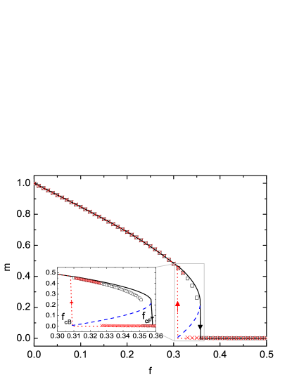
Figure 3: (Color online). Comparison between mean-field theory and MC simulations for phase transition curve $m\sim f$ in the type-I three-state MV model on ER networks. Lines correspond to the theoretical results, and symbols to simulation ones. The networks parameters used in the simulation are $N=5\times 10^{5}$ and $\left\langle k\right\rangle=10$. Within the hysteresis region, $m$ has two stable solutions (black solid line and red dotted line) and one unstable solution (blue dashed line). The inset shows an enlargement for the hysteresis region.

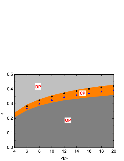
Figure 4: (Color online). Phase diagram in the type-I three-state MV model on ER networks with different average degree $\left\langle k\right\rangle$. The phase diagram is divided into three regions: ordered phase (OP), disordered phase (DP), and coexisting phase (CP). Symbols denote the simulation results on ER networks with $N=5\times 10^{5}$: $f_{cF}$ (cycles) and $f_{cB}$ (triangles).

In Fig. 3, we show the theoretical results (lines) of the type-I three-state MV model on ER random networks whose degree distribution follows the Poisson distribution $P(k)={e^{-\left\langle k\right\rangle}}{\left\langle k\right\rangle^{k}}/k!$ with the average degree $\left\langle k\right\rangle=10$. The theoretical calculation suggests that the type-I three-state MV model undergoes a first-order order-disorder phase transition as $f$ varies. For $f<f_{cB}$, the only ordered phase with $m>0$ is stable. For $f>f_{cF}$, the only disordered phase with $m=0$ is stable. In the region $f_{cB}<f<f_{cF}$ (see the inset of Fig. 3 for an enlargement), two metastable phases with $m=0$ and $m>0$ coexist, separated by an unstable state (dashed line). This leads to a hysteresis phenomenon that is typical for a first-order phase transition. For comparison, we also show the simulation results for $N=5\times 10^{5}$ in Fig. 3. There is excellent agreement between our theory and the simulation outside of the hysteresis region. However, a discrepancy exists between theory and simulation for the prediction of phase transition points. One of the main reasons may be that near phase transition points the lifetime of one of the metastable states becomes short so that the metastable state can not be fully sampled in the simulation. This is clearly realized in Fig. 1: the simulation shows that $f_{cB}$ shifts to a smaller value and $f_{cF}$ to a larger value as $N$ increases.

We consider the effect of the average degree $\left\langle k\right\rangle$ on the phase transition in the type-I three-state MV model. The results are summarized in Fig. 4. The phase diagram is divided into three regions: the ordered phase (OP), the disordered phase (DP), and the coexisting phase (CP) of OP and DP. With the increase in $\left\langle k\right\rangle$, the coexisting region is expanded and both the transition points shift to larger values. The simulation results for $N=5\times 10^{5}$ are also added into Fig. 4, which agrees qualitatively with the theoretical prediction.

We now demonstrate the nature of phase transitions for $p>3$. We perform the theoretical calculation and MC simulation on ER networks with $N=5\times 10^{5}$ and $\left\langle k\right\rangle=10$ up to $p=7$. For larger $p$, our theory is computationally prohibitive since the high-dimensional summation in Eq.(8) and Eq.(9) is time-consuming. The results show that for all $p\geq 3$ the phase transitions are of the first-order nature. The phase transition points are shown in Table 1, from which one can see that $f_{cB}$ is almost unaffected by $p$, and $f_{cF}$ increases monotonically with $p$ and approaches 0.5 as $p\rightarrow\infty$.

Table 1: Phase transitions in the type-I $p$-state MV model on ER networks. For $p\geq 3$, the phase transitions are first order, essentially different from the second-order phase transition in the two-state MV model. The simulation results are obtained on networks with the size $N=5\times 10^{5}$ and average degree $\left\langle k\right\rangle=10$.

$p$	order	$f_{cB}$		$f_{cF}$
		theo	simu	theo	simu
2	2nd	0.3091	0.296	N/A	N/A
3	1st	0.3059	0.327	0.3573	0.350
4	1st	0.3043	0.339	0.4067	0.398
5	1st	0.3038	0.350	0.4429	0.434
6	1st	0.3041	0.359	0.4703	0.461
7	1st	0.3055	0.360	0.4918	0.483

To consider the effect of degree heterogeneity on phase transition in the type-I $p$-state MV model, we will show the results on scale-free networks with degree distribution $P(k)\sim k^{-\gamma}$. The networks are generated by the configuration model Newman et al. (2001). Each node is first assigned a number of stubs $k$ that are drawn from a given degree distribution. Pairs of unlinked stubs are then randomly joined. This construction eliminates the degree correlations between neighboring nodes. Finally, we adopt an algorithm to reshuffle self-loops and parallel edges that ensures the degree distribution is unchanged PRE.70.06610. In Fig. 5, we show $m$ as a function of $f$ for several distinct $\gamma$. The larger $\gamma$ is, the more heterogeneous the network is. The network size and the minimal degree of nodes are fixed, $N=2\times 10^{5}$ and $k_{min}=5$. One can see that the nature of first-order phase transition does not change with $\gamma$. As $\gamma$ increases, the jumps in $m$ at phase transition points, $f_{cF}$ and $f_{cB}$ are depressed. We have also considered some other $p$ and found that the main conclusions are the same.

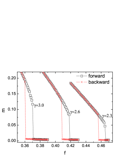
Figure 5: (Color online). Phase transition in the type-I three-state MV model on scale-free networks with degree distribution $P(k)\sim k^{-\gamma}$. From left to right, the degree distribution exponent $\gamma=3.0$, 2.6, and 2.3. A larger $\gamma$ implies that the network has higher degree heterogeneity. The results show that degree heterogeneity suppresses the jump of magnetization near phase transitions. The network size is $N=2\times 10^{5}$ and the minimal degree is $k_{min}=5$. Squares ($\Box$) and crosses ($\times$) correspond to forward and backward simulations, respectively.

III.2 Type-II dynamics

In this subsection, we consider the phase transitions in the type-II $p$-state MV model. As shown in Fig. 6(a) for $p=3$, we find that the forward and backward simulations coincide up to $N=5\times 10^{5}$. This is a feature of continuous phase transition, in agreement with Melo et al. (2010), but in contrast with the result of the type-I three-state MV model shown in Fig. 1. It is interesting that such a small dynamical difference can lead to the essential difference in the nature of phase transition in the three-state MV model. For $p=4$, 5 and 6, as shown in Fig. 6(b-d), we find that the phase transitions are discontinuous, coinciding with the type-I dynamics.

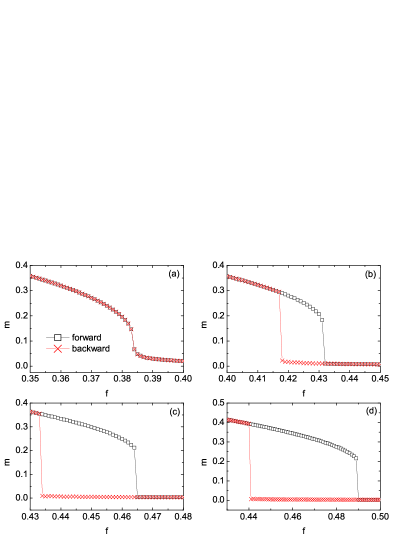
Figure 6: (Color online). Phase transition in the type-II $p$-state MV model on ER networks. From (a) to (d), the numbers of states are $p=3$, $4$, $5$, and $6$, respectively. For the type-II dynamics on ER networks, the phase transition is first order for $p=3$ and second order for $p\geq 4$. The network size is fixed at $N=5\times 10^{5}$. Squares ($\Box$) and crosses ($\times$) correspond to forward and backward simulations, respectively.

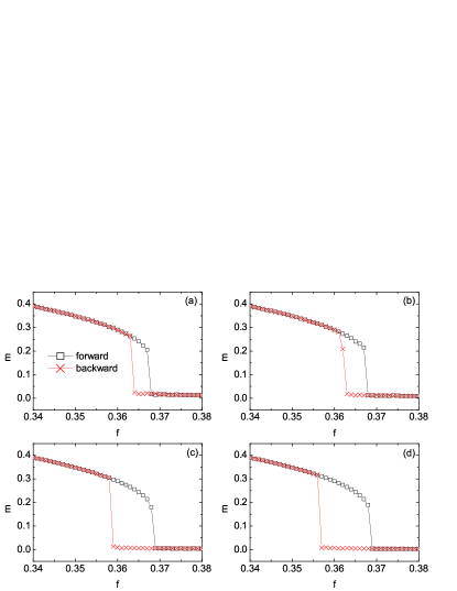
Figure 7: (Color online). First-order phase transition in the type-II three-state MV model on degree-regular random networks, as opposed to the second-order phase transition on ER networks shown in Fig. 6(a). This shows that the order of phase transition in the three-state MV model for the type-II dynamics depends on the heterogeneity of degree distribution. From (a) to (d), the network sizes are $N=5\times 10^{4}$, $10^{5}$, $5\times 10^{5}$, and $10^{6}$, respectively. The degree of each node is exactly equal to $k=10$. Squares ($\Box$) and crosses ($\times$) correspond to forward and backward simulations, respectively.

Moreover, as shown in Fig. 5, the degree heterogeneity can suppress the discontinuity of magnetization at phase transition. A natural question arises: Does a first-order phase transition happen in more homogeneous networks than ER ones when the type-II dynamics is taken into account? For this purpose, we show in Fig. 7 the three-state MV model on degree-regular random networks. Interestingly, the phase transition now becomes first order. That is, the nature of phase transition in the type-II three-state MV model depends on the degree heterogeneity of the underlying networks.

IV Conclusions and Discussion

In conclusion, we have studied numerically and theoretically the order-disorder phase transitions in a $p$-state MV model on complex networks. We find that for $p\geq 3$ the phase transition is of a first-order nature, significantly different from the second-order phase transition in the original two-state MV model. A main feature of the first-order phase transition is the occurrence of a hysteresis loop as noise intensity goes forward and backward. Within the hysteresis region, the ordered phase and disordered phase are coexisting, and the rare phase flips can be observed due to the finite-size fluctuation. The effects of the average degree and the number $p$ of states on the two transition noises (i.e., the boundaries of the hysteresis loop) are investigated. Also, we find that degree heterogeneity can suppress the jump of magnetization at phase transition. Moreover, we compare our model with that introduced in Brunstein and Tomé (1999); Tomé and Petri (2002); Melo et al. (2010). In spite of a small difference in the dynamics, the types of phase transitions in the three-state MV model on ER graphs are essentially different. Interestingly, the phase transition for the latter dynamics becomes first-order on degree-regular random networks. Therefore, the dynamical rule and connectivity heterogeneity between agents play important roles in the order of phase transitions in the three-state MV model.