Magnetization reversal driven by low dimensional chaos in a nanoscale ferromagnet

Abstract

Energy-efficient switching of magnetization is a central problem in nonvolatile magnetic storage and magnetic neuromorphic computing. In the past two decades, several efficient methods of magnetic switching were demonstrated including spin torque, magneto-electric, and microwave-assisted switching mechanisms. Here we report the discovery of a new mechanism giving rise to magnetic switching. We experimentally show that low-dimensional magnetic chaos induced by alternating spin torque can strongly increase the rate of thermally-activated magnetic switching in a nanoscale ferromagnet. This mechanism exhibits a well-pronounced threshold character in spin torque amplitude and its efficiency increases with decreasing spin torque frequency. We present analytical and numerical calculations that quantitatively explain these experimental findings and reveal the key role played by low-dimensional magnetic chaos near saddle equilibria in enhancement of the switching rate. Our work unveils an important interplay between chaos and stochasticity in the energy assisted switching of magnetic nanosystems and paves the way towards improved energy efficiency of spin torque memory and logic.

The striking complexity that may arise in the trajectories of a nonlinear deterministic dynamical system was discovered by Henri Poincaré in the 1880s while studying the three-body problem of celestial mechanics Poincaré (1890). This pioneering work demonstrated strong sensitivity of the dynamic trajectories to small perturbations and gave birth to a branch of science that studies chaos – deterministic dynamics extremely sensitive to initial conditions Li and Yorke (1975); Gleick (1987). The ideas of Poincaré led to the development of Kolmogorov–Arnold–Moser (KAM) theory Arnold et al. (2006), which describes the emergence of chaotic dynamics arising from perturbations applied to integrable Hamiltonian systems. It is now well established that chaotic dynamics is ubiquitous – it is often encountered in celestial mechanics, biology, fluid dynamics, astronomy, as well as mechanical and radio engineering Strogatz (1994). Notably, fluid turbulence – the central problem in aerospace engineering – can be viewed as a manifestation of chaotic dynamics Ruelle and Takens (1971). From the fundamental point of view, the chaotic nature of molecular dynamics has played a key role in establishing rigorous foundations of statistical mechanics in connection with the ergodic hypothesis and the law of increase of entropy Castiglione et al. (2008).

Remarkably, chaos may already arise in dynamical systems with a few degrees of freedom, such as systems described by three state variables or by two state variables in the presence of a time-varying external excitation Perko (2001). These low-dimensional dynamical systems are particularly important for studies of chaos because time evolution of all state variables can be traceable in both experiments and numerical simulations performed for such testbed systems Moon (2004).

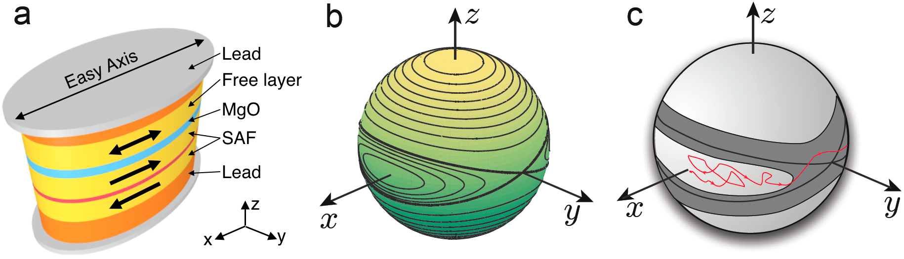
Figure 1: Device and free layer energy landscape. a, Schematics of nanoscale magnetic tunnel junction consisting of a synthetic antiferromagnet (SAF) reference and a superparamagnetic Co₆₀Fe₂₀B₂₀ free layer separated by an MgO tunnel barrier. b, Unit sphere representing the free layer magnetization direction $\bm{m}$ with contour lines of constant magnetic anisotropy energy. The biaxial magnetic anisotropy energy landscape consists of two energy minima at $\bm{m}$ parallel to the $x$-axis, two energy maxima at $\bm{m}$ parallel to the $z$-axis and two saddle points for $\bm{m}$ parallel to the $y$-axis. c, Schematic illustration of the effect of ac spin torque on thermally activated switching of the free layer. The free layer nanomagnet switching trajectory $\bm{m}(t)$ must pass through the dark grey band induced by ac spin torque where deterministic magnetization trajectories connect the two potential wells. The presence of this band of chaotic dynamics results in erosion of the boundary between the two potential wells and reduction of the effective energy barrier for thermally activated switching of magnetization between the wells.

In the field of magnetism, chaotic dynamics was previously observed in ferromagnetic resonance (FMR) experiments at high excitation power Gibson and Jeffries (1984). In FMR measurements, magnetization dynamics is excited by a microwave frequency ac magnetic field applied to a macroscopic ferromagnetic body Montoya et al. (2015). At low ac power levels, only the spatially uniform mode of the magnetic precession is excited resulting in periodic motion of the magnetization at the frequency of the ac drive. When ac power increases above a threshold value, nonlinear coupling of the uniform mode to a continuum of spatially non-uniform spin wave modes gives rise to an exponential growth of the amplitude of multiple modes Suhl (1957). The resulting dynamic state of magnetization is a continuum of interacting large-amplitude spin waves that can exhibit quasi-periodic, chaotic, and turbulent types of dynamics Wigen (1994); L’vov (1994); Iacocca et al. (2015). Such nonlinear magnetization dynamics is currently a very active area of study Podbielski et al. (2007); Guo et al. (2015); Seinige et al. (2015).

While much work was done towards understanding of chaotic dynamics in magnetic systems with continuous degrees of freedom Wigen (1994); L’vov (1994), experimental studies of chaos in magnetic systems with a few degrees of freedom are lacking. In this article, we experimentally and theoretically investigate chaotic dynamics in a ferromagnetic system with two degrees of freedom subject to a periodic external drive. This low-dimensional magnetic chaos is achieved in a magnetic nanoparticle driven by alternating spin transfer torque.

Geometric confinement discretizes the spectrum of spin wave eigenmodes in a nanomagnet and thereby suppresses energy- and momentum-conserving nonlinear spin wave interactions present in bulk ferromagnets with continuous spin wave spectrum Ferona and Camley (2017). This suppression of nonlinear spin wave interactions allows for excitation of large-amplitude quasi-uniform precession of magnetization without simultaneous excitation of other spin wave modes of the system Bertotti et al. (2001); Lee et al. (2010). We demonstrate that this type of magnetic dynamics specific to nanoscale ferromagnets provides a perfect testbed for studies of low-dimensional magnetic chaos Álvarez et al. (2000); Li et al. (2006); Bertotti et al. (2009).

Our studies reveal that chaotic magnetization dynamics induced by alternating spin torque has profound effect on thermally-assisted switching of magnetization in a nanomagnet. This intriguing coupling between low-dimensional deterministic chaos and temperature-induced stochastic dynamicsPufall et al. (2004); Cheng et al. (2010); Rowlands et al. (2013) is not only of fundamental interest but also of significant practical importance. Indeed, novel non-volatile magnetic storage technologies such as spin transfer torque memory (STT-RAM) Sun et al. (2013); Kent and Worledge (2015); Gopman et al. (2014) and microwave-assisted magnetic recording (MAMR Florez et al. (2008); Zhu et al. (2008); Lu et al. (2013)) rely on thermally activated switching of nanoscale ferromagnets. Additionally, innovative computing schemes, such as neuromorphic computing Locatelli et al. (2013) and invertible logic Camsari et al. (2017), have been proposed in such systems in the telegraphic switching regime. Our work reveals that low-dimensional deterministic chaos can be employed for reduction of the effective magnetic energy barrier for switching of magnetization in a nanoscale ferromagnet and thereby paves the way towards more energy-efficient nonvolatile magnetic storage and logic technologies.

Low dimensional chaos in a nanomagnet

In this article, we present experimental and theoretical studies of low-dimensional chaos in a nanoscale ferromagnet with biaxial magnetic anisotropy. The nanomagnet is a 1.8 nm thick Co₆₀Fe₂₀B₂₀ elliptical thin-film element with lateral dimensions of $50\times 75$ nm² that is sufficiently small to support a single-domain ground state. We detect the direction of the nanomagnet magnetization electrically via embedding the nanomagnet as a free layer into a nanoscale magnetic tunnel junction (MTJ) illustrated in Fig. 1a. Rotation of the free layer magnetization with respect to the synthetic antiferromagnet (SAF) reference layers results in variation of the MTJ resistance via tunneling magneto-resistance (TMR) effect Wolf (2001); Ikeda et al. (2007). Since directions of the magnetic moments within the SAF are fixed Wolf (2001); Ikeda et al. (2007), variation of the MTJ resistance with time arises solely from magnetization dynamics of the free layer.

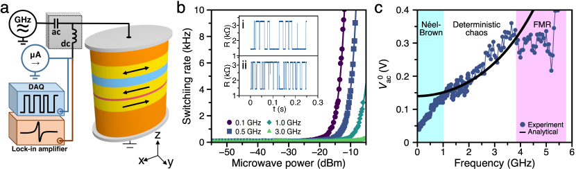
Figure 2: Random telegraph noise measurements. a, Schematics for random telegraph noise (blue) and spin torque ferromagnetic resonance (brown) experiments. b, Dependence of the free layer switching rate $w$ on applied microwave ac power and frequency. The solid lines are guides to the eye. The insets show resistance of the MTJ as a function of time measured at two values of a 0.5 GHz ac power: (i) $P_{\mathrm{ac}}=-55$ dBm and (ii) $P_{\mathrm{ac}}=-18.5$ dBm. c, Threshold ac drive voltage $V_{\mathrm{ac}}^{0}$ as a function of the ac drive frequency. The black solid line is theoretical prediction for the onset of ac-driven chaotic dynamics evaluated analytically at zero temperature.

The direction of the free layer magnetization can be described by a vector $\bm{m}$ on a unit-sphere as shown in Fig. 1b. Dipolar interactions give rise to magnetic shape anisotropy of the nanomagnet that is predominantly easy-plane with its hard axis along the film normal Beleggia et al. (2006). A weaker easy-axis anisotropy is present in the sample plane with its easy axis parallel to the long axis of the ellipse. The biaxial anisotropy energy landscape of this system with two degrees of freedom can be visualized by drawing constant-energy contours on the unit sphere (Fig. 1b). This landscape consists of two magnetic potential energy wells near the energy minima at $m_{x}=\pm 1$ and two saddle points at $m_{y}=\pm 1$. The constant energy contours passing through the saddle points (thick black lines in Fig. 1b) are separatrices that form the boundaries of the potential wells.

In the following sections we show that chaotic magnetization dynamics of the free layer nanomagnet can be induced by ac spin torque when $\bm{m}$ passes sufficiently close to the separatrices. Specifically, chaotic dynamics is realized within a band of anisotropy energies around the separatrix energy (dark gray band in Fig. 1c). The width of this band of chaotic dynamics increases with increasing amplitude of the ac drive Serpico et al. (2015); d’Aquino et al. (2016). Infinitesimal changes of the initial direction of $\bm{m}$ within this energy band are predicted to result in strong variation of the magnetization trajectory, which is the main signature of deterministic chaos.

The process of magnetization switching from one potential well into the other necessarily involves crossing the separatrices and, therefore, must proceed via the band of chaotic dynamics induced by the ac drive. Therefore, we expect the ac-driven chaotic dynamics to affect the nanomagnet switching behavior. In this article, we experimentally investigate thermally activated switching between the potential wells schematically illustrated by a stochastic trajectory in Fig. 1c (red line). We study the effect of ac spin torque drive on the rate of thermally activated switching of the free layer nanomagnet and thereby probe the effect of chaotic dynamics on the switching process.

Experimental results

In order to accelerate measurements of thermally-activated switching of the free layer nanomagnet, we employ MTJ samples with superparamagnetic free layers Locatelli et al. (2014), in which the free layer stochastically switches between the two anisotropy energy wells at the rate of several tens of Hz. This system exhibiting random telegraph noise (RTN) Pufall et al. (2004); Costanzi and Dahlberg (2017) allows us to collect statistically accurate data on thermally activated switching rates and their modification by ac spin torque over experimentally convenient time of several hours at room temperature.

The high value of tunneling magnetoresistance (TMR) of the MTJ spin-valve allows us to monitor the RTN dynamics of the free layer in real time. The experimental setup for the RTN measurements is shown in Fig. 2a. A low-level probe current (-25 $\mu$A) is applied to the MTJ and the voltage across the device is measured by a high-performance DAQ in real time (Methods). In these measurements, we apply a small in-plane magnetic field (3.7 mT) along the nanomagnet easy axis that compensates the stray field from the SAF layer acting onto the free layer and balances the dwell times of the free layer in the high-resistance (antiparallel, AP) and low-resistance (parallel, P) states. A microwave frequency ac voltage applied to the MTJ via the ac port of the bias tee gives rise to an ac spin torque applied to the free layer by spin-polarized electric current from the SAF layer. The switching rate of the free layer nanomagnet is the inverse of the dwell time $w\equiv 1/\tau$. Examples of time-domain RTN data are shown in the insets of Fig. 2b.

Example of the measured switching rate dependence on the applied microwave power $P_{\mathrm{ac}}$ is shown in Fig. 2b for the ac spin torque frequencies $f=0.1$, 0.5, 1.0, and 3.0 GHz. All these frequencies lie below the FMR frequency of the free layer $f_{\mathrm{FMR}}=5.1$ GHz (Supplementary Note 1), as determined from field-modulated spin torque ferromagnetic resonance (ST-FMR) measurements (Methods)Gonçalves et al. (2013).

The RTN data in Fig. 2b reveal that the switching rate of the free layer is strongly affected by ac spin toque with frequencies well below the FMR frequency of the free layer. Furthermore, lower frequencies of the ac drive have stronger effect on the switching rate. These data clearly show that the observed effect of the ac drive on switching is not connected to the resonant excitation of the free layer magnetization (FMR). We argue that the observed effect of the low-frequency ac drive arises from the low dimensional chaotic dynamics induced by the ac spin torque.

The data in Fig. 2b clearly show that the effect of ac spin torque on the free layer switching has a threshold character in the ac power. These data also reveal that the threshold power decreases with decreasing frequency of the ac drive. In order to quantify the dependence of the threshold power on the ac drive frequency, we define the threshold power $P_{\mathrm{ac}}^{0}$ as the ac power at which the switching rate $w$ doubles compared to its value in the absence of the ac drive.

Fig. 2c shows frequency dependence of the ac threshold voltage $V_{\mathrm{ac}}^{0}$ applied to the sample calculated from the measured threshold power $P_{\mathrm{ac}}$ by correcting for frequency-dependent attenuation in the measurement circuit and impedance-dependent ac signal reflection from the sample Pozar (2005). The black solid line in Fig. 2c shows our zero-temperature theoretical prediction (discussed in the next section) for frequency dependence of the ac threshold voltage for the onset of chaotic magnetization dynamics. The prediction is in good agreement with our experimental data in a wide range of ac frequencies (1-4 GHz) below the FMR frequency. The deviations from the analytic prediction at higher and lower frequencies will be addressed in the Discussion section.

Theory

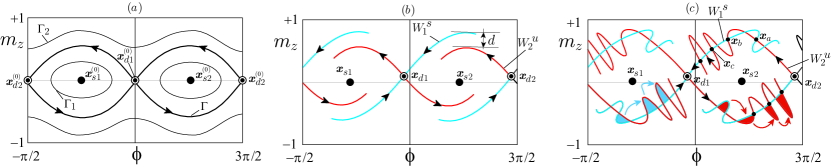
Figure 3: Qualitative sketches of the magnetization trajectories in the $(\phi,m_{z})$-plane. ($\phi$ is the azimuthal angle around the $z$-axis). a, Conservative trajectories ($\alpha=0,\beta_{\mathrm{ac}}=0$, designated by superscript ⁽⁰⁾). $\Gamma_{1},\Gamma_{2}$ are constant energy trajectories and $\Gamma$ is the heteroclinic trajectory (separatrix). b, Damping dominated dynamics ($\alpha>0,\beta_{\mathrm{ac}}<\beta^{\mathrm{crit}}_{x}$, $d>0$). Here $\bm{x}_{d1},\bm{x}_{d2}$ are saddle equilibria; $\bm{x}_{s1},\bm{x}_{s2}$ are node-type equilibria; $W^{s}_{1}$ is stable manifold associated with $\bm{x}_{d1}$; $W^{u}_{2}$ is unstable manifold associated with $\bm{x}_{d2}$; $d$ is the splitting of the manifolds. c, Heteroclinic tangle formation ($\alpha>0,\beta_{\mathrm{ac}}>\beta^{\mathrm{crit}}_{x}$). The manifold intersection points $\bm{x}_{a},\bm{x}_{b},\bm{x}_{c}$ are generated by iterating the stroboscopic map equation (3). Intersecting stable and unstable manifolds form lobes. Blue regions indicate capturing lobes that keep the magnetization inside the given potential well while red regions show escaping lobes that bring magnetization outside of the well. The colored arrows indicate the transformation of one lobe into another under the action of the map equation (3).

From a theoretical point of view, the chaotic magnetization dynamics induced by ac torque can be studied with tools of nonlinear dynamical systems such as the Poincaré map Serpico et al. (2015). Such analysis allows the definition of the concept of erosion of the stability region of magnetic equilibria by the ac drive d’Aquino et al. (2016), which provides a natural connection between deterministic chaos and thermally-activated switching over the energy barrier.

Magnetization dynamics for a uniformly magnetized particle driven by spin torque is described by the stochastic Landau-Lifshitz equation Kubo and Hashitsume (1970); Mayergoyz et al. (2009):

$$\frac{d\bm{m}}{dt}=-\bm{m}\times\left(\bm{h}_{\mathrm{eff}}+\alpha\left(\bm{m}\times\bm{h}_{\mathrm{eff}}\right)-\beta\left(\bm{m}\times\bm{e}_{\mathrm{p}}\right)+\nu\bm{h}_{\mathrm{N}}\right),$$ (1)

where $\bm{m}$ is the magnetization vector of unit length $|\bm{m}|=1$ (normalized by the saturation magnetization $M_{\mathrm{s}}$), time is measured in units of $(\gamma M_{\mathrm{s}})^{-1}$ ($\gamma$ is the absolute value of the gyromagnetic ratio), $\bm{h}_{\mathrm{eff}}=-\partial g/\partial\bm{m}$ is the effective field, $g=g(\bm{m},\bm{h}_{\mathrm{a}})$ is the magnetic free energy, $\bm{h}_{\mathrm{a}}$ is the external magnetic field, $\alpha$ is the damping constant, $\beta(t)=\beta_{\mathrm{ac}}\cos(\omega t)$ is the normalized ac Slonczewski spin torque Mayergoyz et al. (2009) ($\beta_{\mathrm{ac}}=2\lambda J_{\mathrm{ac}}/J_{\mathrm{p}}$, with $J_{\mathrm{ac}},\lambda,\bm{e}_{\mathrm{p}}$ being injected current density, spin polarization factor, polarizer unit-vector, respectively) and $J_{\mathrm{p}}=|e|\gamma M_{\mathrm{s}}^{2}t_{\mathrm{FL}}/(g_{\mathrm{L}}\mu_{\mathrm{B}})$ is an intrinsic current density value depending on free layer saturation magnetization $M_{\mathrm{s}}$ and thickness $t_{\mathrm{FL}}$ ($e$ is the electron charge, $g_{\mathrm{L}}\approx 2$ is the Landé factor, $\mu_{\mathrm{B}}$ is the Bohr magneton), $\nu$ is the thermal noise intensity, and $\bm{h}_{\mathrm{N}}(t)$ is the standard isotropic Gaussian white-noise stochastic process. The energy function $g$, measured in units of $\mu_{0}M_{\mathrm{s}}^{2}V$ ($\mu_{0}$ is the vacuum permeability and $V$ the volume of the particle), is given by:

$$g(\bm{m},\bm{h}_{\mathrm{a}})=\frac{1}{2}D_{x}m_{x}^{2}+\frac{1}{2}D_{y}m_{y}^{2}+\frac{1}{2}D_{z}m_{z}^{2}-\bm{m}\cdot\bm{h}_{\mathrm{a}}$$ (2)

where $D_{x}$, $D_{y}$, $D_{z}$ are the biaxial anisotropy constants. The intensity of the thermal noise $\nu$ is connected to the damping $\alpha$ in accordance with the fluctuation-dissipation theorem Mayergoyz et al. (2009), i.e. $\nu^{2}=(2\alpha k_{\mathrm{B}}T)/(\mu_{0}M_{\mathrm{s}}^{2}V)$, where $T$ is the absolute temperature of the thermal bath and $k_{\mathrm{B}}$ is the Boltzmann constant.

We initially solve the Landau-Lifshitz equation in the absence of thermal noise $(\nu=0)$ in order to elucidate the role of deterministic chaos for the system of interest. Magnetization on the unit sphere described by equation (1) (with $\nu=0$) is a two dimensional dynamical system of nonautonomous type since the right-hand-side of the equation depends explicitly and periodically on time. This type of dynamics can be conveniently studied by introducing the stroboscopic map $P[\cdot]$, defined as Ott (2002):

$$\bm{m}_{n+1}=P[\bm{m}_{n}]\,,$$ (3)

where $\bm{m}_{n}=\bm{m}(t_{0}+n\,T_{\mathrm{ac}})$, and $T_{\mathrm{ac}}={2\pi}/{\omega}$, which maps an initial magnetization $\bm{m}(t_{0})$ to the magnetization $\bm{m}(t_{0}+T_{\mathrm{ac}})$ obtained by integrating equation (1) (with $\nu=0$) over a time interval equal to the period $T_{\mathrm{ac}}$ of the ac drive.

The mathematical form of the stroboscopic map cannot be derived in closed form, but certain features of the map dynamics can be obtained when the damping and the applied spin torque are small. In this case, the map describes the perturbation of the conservative dynamics described by equation (1) when $\alpha=0$, $\beta_{\mathrm{ac}}=0$, and $\nu=0$. The time evolution of magnetization in the conservative dynamics follows the constant energy contours, which are sketched in Fig. 3a. A crucial role in the conservative dynamics, equation (3), is played by the saddle equilibria points ($\bm{x}_{d1}^{(0)}$, $\bm{x}_{d2}^{(0)}$) heteroclinically connected by separatrices that mark the boundaries of the two potential wells (Fig. 3a).

For non-zero damping and spin torque ($\alpha\neq 0$, $\beta_{\mathrm{ac}}\neq 0$), the saddle points of the map ($\bm{x}_{d1}$, $\bm{x}_{d2}$) are the origin of lines, referred to as stable and unstable manifolds, that play analogous role to the separatrices of the conservative case ($\alpha=0$, $\beta_{\mathrm{ac}}=0$) and thereby provide structure to the state space (see Fig. 3b). The stable manifolds $W_{1}^{s}$, $W_{2}^{s}$ are sets (curves) of all initial conditions which under the action of the map (equation (3)) approach the saddles $\bm{x}_{d1}$, $\bm{x}_{d2}$, respectively. The unstable manifolds $W_{1}^{u}$, $W_{2}^{u}$ are sets (curves) of all initial conditions which under backward flow of time on the stroboscopic map (equation (3)) approach the saddles $\bm{x}_{d1}$, $\bm{x}_{d2}$, respectively. These manifolds are invariant sets, which means that they contain all forward and backward map iterates of points taken on them.

In Fig. 3b, the two manifolds $W_{1}^{s}$ and $W_{2}^{u}$ are sketched and their splitting is indicated by $d$. This splitting depends on the value of damping and ac spin torque, and it may vanish for a sufficiently large ac spin torque amplitude. When this occurs, a point of intersection $\bm{x}_{a}$ belonging to both invariant sets $W_{1}^{s}$ and $W_{2}^{u}$ emerges (see Fig. 3c). This implies that forward and backward iterates of $P[\cdot]$ starting from $\bm{x}_{a}$ must belong to $W_{1}^{s}\cap W_{2}^{u}$ and thus that the two curves $W_{1}^{s}$, $W_{2}^{u}$ must intersect an infinite number of times (see Fig. 3c). This phenomenon is referred to as heteroclinic tangle (chaotic saddle) and is responsible for chaotic and unpredictable dynamic behavior of the system near the saddles. This chaotic dynamics can be illustrated in terms of lobe dynamics. Regions of the state space bounded by segments of stable and unstable manifolds of the saddles form lobes, examples of which are the colored regions in Fig. 3c. Under the action of the map, one lobe transforms into another. There are two classes of lobes: the escaping ones (marked by red color), which tend to bring points outside the well, and the capturing lobes (marked by blue color), which tend to bring points inside the well. Escaping and capturing lobes do actually finely intersect possibly a denumerable amount of times, and this gives rise to a fractal boundary between the points which enter the well and points which escape the well Ott (2002). The region in which lobes formed by the stable and unstable manifold intersect is the region where chaotic saddle dynamics takes place.

For sufficiently small applied torques and damping, the splitting $d$ can be analytically derived by using the Melnikov function technique Holmes (1979); Mel’nikov (1963) and one can calculate the threshold ac torque Nusse and Yorke (1989); Tyrkiel (2005) at which the splitting becomes zero and the saddle becomes chaotic. Such threshold values of $\beta_{\mathrm{ac}}$ for the onset of the heteroclinic tangle, for spin current polarized along each of the anisotropy principle axes are: Serpico et al. (2015):

$$\beta_{x}^{\text{crit}}=\beta_{\text{opt}}^{\text{crit}}/k^{\prime},\quad\beta_{y}^{\text{crit}}=\infty,\quad\beta_{z}^{\text{crit}}=\beta_{\text{opt}}^{\text{crit}}/k\,\,,$$ (4)

$$\beta_{\text{opt}}^{\text{crit}}=\frac{2\alpha\varOmega_{d}}{\pi}\cosh\frac{\pi\omega}{2\varOmega_{d}}\,\,,$$

where $k^{2}=(D_{z}-D_{y})/(D_{z}-D_{x})$, $k^{\prime 2}=1-k^{2}$, $\varOmega_{d}=\sqrt{\smash[b]{(D_{z}-D_{y})(D_{y}-D_{x})}}$. The infinite result for the case of $y$-polarization is due to the fact that the method is first order accurate with respect to perturbation amplitudes $\alpha,\beta$. The result implies that a spin polarization along the $y$ axis produces a much weaker effect with respect to other orientations. In our experiment, the spin polarization vector set by the SAF magnetic moment direction is parallel to the $x$ axis, which means that the critical ac spin torque value needed to induce chaotic magnetization dynamics in our MTJ system is $\beta_{x}^{\text{crit}}$.

Using Eq. (4), we calculate the zero-temperature threshold ac voltage for the onset of heteroclinic tangle $V_{\mathrm{ac}}^{0}(f)$. For the conversion from dimensionless to physical units, we remark that a spin-torque amplitude $\beta_{x}^{\text{crit}}=1$ corresponds to an ac voltage $V_{\mathrm{ac}}^{0}=15.5$ V and a dimensionless angular frequency $\omega=1$ corresponds to a frequency $f=30.8$ GHz (see Methods for details). Thus, the calculated threshold voltage $V_{\mathrm{ac}}^{0}(f)$ is compared to the measured threshold voltage in Fig. 2c.

Discussion

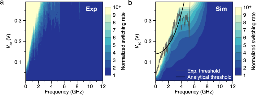
Figure 4: Room temperature free layer switching rate. The rate is mapped as a function of the applied ac voltage $V_{\mathrm{ac}}$ and frequency $f$ for (a) experiment and (b) numerical solution of the stochastic LLG equation (Eq. (1)). The black line overlayed on (b) is analytical prediction of the threshold voltage for the onset of zero-temperature chaotic dynamics due to heteroclinic tangle, while the grey line is experimentally measured threshold voltage obtained from the experimental data in (a).

The agreement between the measured and theoretically predicted threshold voltages is excellent in the 1-4 GHz frequency range (region labeled Deterministic chaos in Fig. 2c). The deviations of the threshold voltage from the value predicted by the heteroclinic tangle theory at frequencies below 1 GHz (region labeled Néel-Brown in Fig. 2c) arise from adiabatic enhancement of the amplitude of thermal fluctuations of magnetization by spin torque. When the ac spin torque frequency is lower than the Néel-Brown attempt frequency for thermally activated switching Brown (1963); Suh et al. (2008), antidamping spin torque can significantly amplify the amplitude of thermally-induced magnetization precession in a half-cycle of the ac drive Petit et al. (2007) and thereby induce switching over the energy barrier.

This mechanism of thermally assisted switching is distinctly different from the heteroclinic tangle mechanism and it can significantly decrease the low-frequency value of the ac threshold voltage below that predicted by Eq. (4). To verify the role of this mechanism, we numerically solved d’Aquino et al. (2006) the stochastic LLG equation (1) at T = 300 K (Methods). The results of these simulations shown in Fig. 4b are in a remarkably good agreement with the experimental data shown in Fig. 4a over the entire frequency range employed in the experiment. These simulations confirm that the threshold voltage is significantly reduced by the antidamping action of ac spin torque at frequencies below the attempt frequency but is nearly insensitive to temperature at frequencies exceeding the attempt frequency.

We also observe deviations of the threshold voltage from the value predicted by the heteroclinic tangle theory at frequencies near the FMR frequency (region labeled FMR in Fig. 2c), which can be explained by resonant transfer of energy from the ac spin torque to magnetization at the FMR frequency Montoya et al. (2015). This resonant mechanism of lowering the threshold for thermally activated switching of magnetization is exploited in MAMR technologies Florez et al. (2008); Zhu et al. (2008); Lu et al. (2013). From the data in Fig. 4, one can see that the erosion of the effective energy barrier due to chaos at sub-FMR frequencies is more efficient at leading to magnetization switching than the resonant absorption of energy near the FMR frequency. This implies that deterministic chaos induced by a sub-FMR-frequency drive may be a more energy-efficient approach to energy-assisted switching of magnetization than MAMR at the FMR frequency.

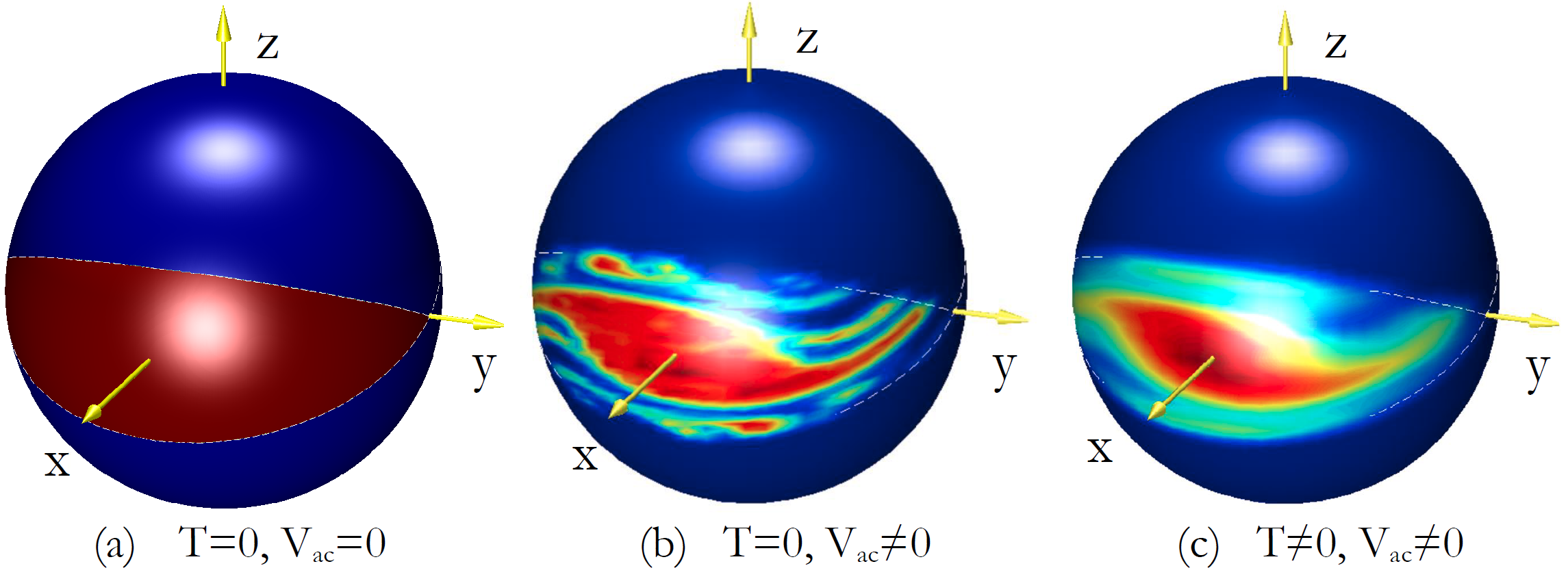
Figure 5: Visualizing chaos. Directional map of probability of magnetization initially within the $x>0$ potential well to remain within this well after 5 periods of alternating spin torque drive. Red color marks the initial direction of magnetization resulting in magnetization staying withing the well, while blue color marks initial magnetization direction resulting in escape from the well after 5 periods of the drive. a, At zero temperature and in the absence of spin torque any initial direction of magnetization within the well indefinitely remains within the well. b, At zero temperature and alternating spin torque exceeding the threshold value, the fractal structure of escaping and capturing lobes within the well near the separatrices is apparent. Colors intermediate between red and blue appear as a result of coarse grained averaging of the fractal lobe structure over a small but finite solid angle. It is clear from this figure that chaotic dynamics induced by alternating spin torque decreases the basin of stability to a region in the center of the well, thereby reducing the effective energy barrier between the two wells. c, At room temperature and spin torque drive exceeding the threshold value, the fractal lobe structure of the well is blurred by thermal fluctuations but the chaos-induced erosion of the basin of stability is still apparent.

It is important to stress that the effect observed in the 1-4 GHz regime is not related to the FMR phenomenon. In FMR type dynamics, magnetization exhibits ac-driven small-angle deviations from the easy axis $m_{x}=\pm 1$, and the ac frequency is close to the FMR frequency. In the present study, we focus on dynamics driven by frequencies substantially lower than the FMR frequency. For sufficiently high ac power, chaotic dynamics is induced when magnetization is almost orthogonal to the easy axis (near $m_{y}=\pm 1$, the saddle critical points of anisotropy energy, as illustrated in Fig. 1b). This regime corresponds to the top of the two potential wells in Fig. 1c, which are rarely visited by magnetization in thermal equilibrium. However, in the process of switching from one well to the other, magnetization must pass near one of the saddle critical points and, for this reason, the switching rate is affected by the ac-driven chaotic dynamics.

From another perspective, such chaotic regime results in partial erosion of the magnetic anisotropy barrier separating two potential wells Thompson (1989). The concept of such barrier erosion, as well as a more detailed picture of the interplay between chaotic dynamics and thermal fluctuations, are illustrated in Fig. 5a-c, which are obtained by numerical simulations of magnetization dynamics (Supplementary Note 2). These figures can be thought of as the actual representation of the qualitative sketch shown in Fig. 1c. By using a color scale, we represent the different degrees of stability of the magnetization states inside a potential well. The degree of stability of a given state is measured by the number of ac-excitation periods after which the trajectory starting from that state leaves the $m_{x}=+1$ potential well. In this figure, red points represent the initial directions of magnetization that do not leave the potential well and, therefore, are states with the highest stability; conversely, points with color toward the blue are those with decreasingly less stability.

In Fig. 5a, for zero temperature and zero ac excitation, stable points fill the entire energy well around the energy minimum along the easy $x$ axis. In Fig. 5b, for zero temperature and sufficiently large ac voltage, fractal instability regions arising from chaotic dynamics appear in the energy well, which reduces the stability margin of the equilibrium. In Fig. 5c, when both ac voltage and temperature are nonzero, the entangled instability regions due to chaos are smoothed out by thermal fluctuations, but the effective erosion of stability margin of the equilibrium remains, which implies a reduction of the barrier for thermally activated switching. With increasing degree of erosion, the thermally activated switching rate dramatically increases. This is the experimentally detectable signature of chaos.

The interplay between such chaotic regime of magnetic dynamics and thermal fluctuations, to our knowledge, has not been studied. It is well-known that the thermal transition (escape) times are described by the Arrhenius law: $\tau=\tau_{0}\exp\left[\Delta E/k_{\mathrm{B}}T\right]$, where $\Delta E$ is the anisotropy energy barrier for switching, and $1/\tau_{0}$ is the attempt frequency Brown (1963). The problem of generalizing the Arrhenius law to the regime of ac-driven chaotic dynamics remains largely open. Our work shows that the effect of chaotic dynamics on the escape rate is detectable in magnetic nanodevices, which should stimulate both experimental and theoretical studies of this important problem.

In contrast to the majority of previous studies of chaotic dynamics focused on steady-state chaotic motion, the chaotic dynamics studied here is of transient type Lai and Tél (2011). This kind of chaos is essentially of the same nature as the one discovered by Poincarè in the three body problem and addressed by KAM theory. However, the magnetic chaos studied here cannot be directly described by KAM theory, which is formulated for conservative systems. Indeed, ac spin torque driving chaotic magnetic dynamics in our MTJ system is manifestly non-conservative (as well as the Gilbert damping torque).

As a general rule, physical systems with multistable energy landscape, which are weakly dissipative and subject to sufficiently large ac excitations, exhibit chaotic dynamics near their saddle equilibria Ott (2002). Nanoscale magnetic devices, such as the MTJs studied in this work, are an important case of this class of systems. The possibility of measuring and controlling magnetization in these devices in real time gives a unique opportunity to study chaotic dynamics. In this work, we explored this opportunity which, to our knowledge, is one of the first clear attempts to detect chaos in nanoscale systems at room temperature. It is remarkable that the analytical calculation based on deterministic dynamics leads to correct predictions of the experimentally measured frequency dependence of the threshold power needed to trigger low dimensional magnetic chaos. Our results are not restricted to the field of nanomagnetism; we expect them to be important in a variety of driven dynamical systems and phenomena such as nanomechanical oscillators Badzey and Mohanty (2005), multistable lasers Larger et al. (2015), and stimulated chemical reactions Croft et al. (2017).

Finally, from the application point of view, energy efficient switching of magnetization is highly desirable for practical spintronic memory and logic devices Schumacher et al. (2003); Khalili Amiri et al. (2011); Nguyen et al. (2018); Chen et al. (2018). Our work shows that ac-driven chaos can facilitate thermally-assisted switching of magnetization, which provides a new pathway towards energy-efficient magnetic nanodevices. For example, nanoscale magnetic tunnel junctions with superparamagnetic free layers are now being exploited in emergent neuromorphic computing Locatelli et al. (2014); Mizrahi et al. (2018). Our results show that low dimensional chaos provides tunability of switching rates in such systems, and as such, may lead to novel computing schemes that simultaneously harness stochasticity and deterministic chaos.

I Acknowledgements

This work was supported by the National Science Foundation through Grants No. DMR-1610146, No. EFMA-1641989 and No. ECCS-1708885. We also acknowledge support by the Army Research Office through Grant No. W911NF-16-1-0472 and Defense Threat Reduction Agency through Grant No. HDTRA1-16-1-0025. This work was also carried on in the framework of Programme for the Support of Individual Research 2016-2017 funded by University of Naples “Parthenope”. We thank Juergen Langer and Berthold Ocker for magnetic multilayer deposition.

II Author contributions

I.N.K, M.d’A., and C.S. planned the study. E.A.M. designed and performed RTN measurements and performed ST-FMR measurements with consultation from Y.-J.C. M.d’A. and C.S. provided numerical simulation code and analytic theory. S.P. performed simulations under the supervision of M.d’A. J.A.K. made the samples. M.d’A., I.N.K, C.S., and E.A.M wrote the manuscript. All authors discussed the results.

III Methods

Sample description. The magnetic tunnel junctions (MTJs) are patterned from (bottom lead)$|$(5)Ta$|$(15)PtMn$|$SAF$|$(0.8)MgO$|$(1.8)CoFeB$|$(2)Cu$|$ (top lead) multilayers (thickness in nm) deposited by magnetron sputtering. Here SAF $\equiv$ (2.5)Co₇₀Fe₃₀$|$(0.85)Ru$|$(2.4)Co₄₀Fe₄₀B₂₀ is the pinned synthetic antiferromagnet, with magnetic moments lying in the sample plane, which is used as both the polarizer and reference layer. The unpatterned multilayers were annealed at a temperature of 300^∘ C in an external field of 10 kOe applied in the sample plane for 2 hours. The elliptical MTJs are patterned such that the major axis (easy ferromagnetic axis) is parallel to the annealing field direction.

Spin torque ferromagnetic resonance. We employ field-modulated spin torque ferromagnetic resonance (ST-FMR) technique to determine $f_{\mathrm{FMR}}$ in our samples Gonçalves et al. (2013); Tulapurkar et al. (2005); Harder et al. (2016). In these measurements, microwave voltage is applied to the MTJ through the ac port of the bias tee, and rectified voltage generated by the MTJ at the frequency of magnetic field modulation is measured by a lock-in amplifier through the DC port of the bias tee, as schematically illustrated in Fig. 2a.

Random telegraph noise measurements. The thermally activated switching rate of the free layer in the MTJ is monitored via random telegraph noise (RTN) measurements. The experimental setup for the RTN measurements is shown in Fig. 2a. A low-level probe current (-25 $\mu$A) is applied to the MTJ and the voltage across the device is measured by a high-performance data acquisition system (DAQ National Instruments USB-6356) in order to monitor the MTJ resistance as a function of time. In these measurements, we apply a small in-plane magnetic field (3.7 mT) along the nanomagnet easy axis that compensates the stray field from the SAF layer acting onto the free layer and balances the dwell times of the free layer in the high-resistance (antiparallel, AP, $3350~{}\Omega$) and low-resistance (parallel, P, $1450~{}\Omega$) states. A microwave frequency ac voltage can be applied to the MTJ via the ac port of the bias tee. This voltage gives rise to an ac spin torque applied to the free layer by spin-polarized electric current from the SAF layer. The dwell times of the P state $\tau_{\textup{P}}$ and the AP state $\tau_{\textup{AP}}$ were found to remain balanced under the ac drive ($\tau_{\textup{AP}}=\tau_{\textup{P}}=\tau$). The switching rate of the free layer nanomagnet is the inverse of the dwell time $w\equiv 1/\tau$.

Numerical simulations The stochastic LLG equation (1) has been repeatedly solvedd’Aquino et al. (2006) for an ensemble of $N=20000$ particle replicas, for given values of $\beta_{\mathrm{ac}}$ and $\omega$ to compute the average switching rates of Fig. 4b. The values of parameters used in simulations are $\mu_{0}M_{\mathrm{s}}=1.1T,D_{x}=0.035,D_{y}=0.056,D_{z}=0.909,\alpha=0.016$. Dimensionless angular frequency $\omega=1$ corresponds to frequency $f=\gamma M_{\mathrm{s}}/(2\pi)=30.789$ GHz, dimensionless ac spin-torque $\beta_{\mathrm{ac}}=1$ corresponds to injected ac current with amplitude $I_{\mathrm{ac}}=J_{\mathrm{p}}S/(2\lambda)=6.5$ mA (polarization factor $\lambda=0.6$, MTJ cross-sectional area $S=2.9452\times 10^{-15}$ m², $J_{\mathrm{p}}=|e|\gamma M_{\mathrm{s}}^{2}t_{\mathrm{FL}}/(g_{\mathrm{L}}\mu_{\mathrm{B}})=2.63\times 10^{12}$ A/m², $t_{\mathrm{FL}}=1.8$ nm). Conversion between current and voltage applied to the MTJ is performed as $V_{\mathrm{ac}}=RI_{\mathrm{ac}}$ where the resistance $R=(R_{\mathrm{P}}+R_{\mathrm{AP}})/2=2400\,\Omega$ is the average between the measured MTJ resistance values in the parallel and anti-parallel states; thus, an ac spin-torque $\beta_{\mathrm{ac}}=1$ corresponds to a voltage $V_{\mathrm{ac}}=2400\,\Omega\times 6.5\,\text{mA}=15.5$ V.

Supplementary Material for Magnetization reversal driven by low dimensional chaos in a nanoscale ferromagnet

Eric Arturo Montoya, Salvatore Perna, Yu-Jin Chen, Jordan A. Katine, Massimiliano d^′Aquino, Claudio Serpico, and Ilya N. Krivorotov

Supplementary Note 1: Spin torque ferromagnetic resonance

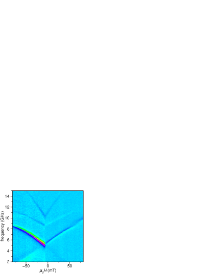
Figure S1: Spin torque ferromagnetic resonance measurement.

We employ field-modulated spin torque ferromagnetic resonance (ST-FMR) technique to determine the ferromagnetic resonance frequency $f_{\mathrm{FMR}}$ in our samples Gonçalves et al. (2013); Tulapurkar et al. (2005). In these measurements, microwave voltage is applied to the MTJ through the ac port of the bias tee, and rectified voltage generated by the MTJ at the frequency of magnetic field modulation is measured by a lock-in amplifier through the DC port of the bias tee, as schematically illustrated in Fig. 2a of the main text. The ST-FMR spectra measured as a function of in-plane magnetic field applied parallel to the free layer easy axis reveal that the lowest frequency mode of the free layer (the quasi-uniform FMR mode) in zero applied field is $f_{\mathrm{FMR}}=5.1$ GHz, as shown in Fig. S1 Gonçalves et al. (2013). A higher order spin wave mode is observed at $f=9$ GHz Gonçalves et al. (2013). In the main text we are mainly concerned with the magnetization dynamics at driving frequencies below $f_{\mathrm{FMR}}$.

Supplementary Note 2: Basin erosion

Figure S2: Quantitative analysis of basin erosion. Top panel A: degree of erosion $\eta$ as a function of ac drive frequency $f$ and voltage $V_{\textup{ac}}$. Lower panels B,C,D,E: numerically computed basin erosion produced in the $(\phi,m_{z})$-plane for $T=0$ and ac spin-torque polarizer along the $x$ direction. The low energy well is initially filled by $N=10^{5}$ phase points. When the trajectory originating from a phase point escapes the well within $n=5$ iterations of the map (3), it is considered ’unsafe’ and disregarded. The remaining phase points correspond to ’safe’ initial conditions. Panels B,C,D,E refer to different ac frequency/amplitude pairs (associated with markers B,C,D,E in top panel A). Values of parameters refer to a MTJ with $75\times 50\times 1.8$ nm³ elliptical free layer for which $\mu_{0}M_{\mathrm{s}}=1.1T,D_{x}=0.035,D_{y}=0.056,D_{z}=0.909,\alpha=0.016$. Dimensionless angular frequency $\omega=1$ corresponds to frequency $f=\gamma M_{\mathrm{s}}/(2\pi)=30.789$ GHz, dimensionless ac spin-torque $\beta_{\mathrm{ac}}=1$ corresponds to injected ac current with amplitude $I_{\mathrm{ac}}=J_{\mathrm{p}}S/(2\lambda)=6.5$ mA (polarization factor $\lambda=0.6$, cross-sectional MTJ area $S=2.9452\times 10^{-15}$ m², $J_{\mathrm{p}}=|e|\gamma M_{\mathrm{s}}^{2}t_{\mathrm{FL}}/(g_{\mathrm{L}}\mu_{\mathrm{B}})=2.63\times 10^{12}$ A/m², $t_{\mathrm{FL}}=1.8$ nm). Conversion between current and voltage applied to the MTJ is performed as $V_{\mathrm{ac}}=RI_{\mathrm{ac}}$ where the resistance $R=(R_{\mathrm{P}}+R_{\mathrm{AP}})/2=2400\Omega$ is the average between the measured MTJ resistance values in the parallel and anti-parallel states (see section Methods); thus, a value of the dimensionless ac spin-torque $\beta_{\mathrm{ac}}=1$ corresponds to an applied voltage $V_{\mathrm{ac}}=2400\Omega\times 6.5\text{mA}=15.5$ V.

A direct consequence arising from the onset of chaotic magnetization dynamics is the phenomenon of erosion of the basins of attraction of asymptotic regimesGilmore and Lefranc (2012), i.e. regions of magnetization dynamics that stay within a given energy well for arbitrarily long times. In fact, the effect of the heteroclinic tangle (chaotic saddle) and the presence of lobes lead to the deterministic escape of magnetization trajectories within the potential well around one free energy minima to outside the well. The erosion has important practical consequences as it is similar to a reduction of the depth of the potential well. Thus, it reduces the ‘safety region’ around a stable equilibrium state. In addition, the boundary of the basin of attraction of asymptotic regimes inside the well acquires a fractal nature.

We stress that the basin erosion phenomenon is of purely deterministic origin and can be studied numericallyThompson (1989); d’Aquino et al. (2016) by iterating the stroboscopic map (main text equation (3)) associated with zero-temperature LLG equation for an ensemble of a very large number $N$ of initial conditions filling one energy well and progressively removing the states that escape the energy well. In this section, we will refer to the energy well around $\bm{m}=+\bm{x}$. Quantitative analysis of the basin erosion can be performed by defining the degree of erosion $\eta$ as the fraction of particles in the ensemble which escape the well in a given number $n$ of iterates of the stroboscopic map d’Aquino et al. (2016). We have performed extensive computations of $\eta$ as function of ac voltage and frequency. The results are reported in the top panel A of Fig. S2. The zero temperature simulations are carried out for $N=10^{5}$ ensemble particles and $n=5$ iterates of the stroboscopic map, and with ac spin-torque polarizer directed along the easy anisotropy axis $x$. Under this ac drive configuration, the ferromagnetic resonance of the nanoparticle is inhibited and, consequently, the excitation of chaotic dynamics is not disturbed by the interplay with magnetic resonance phenomena. Moreover, We have checked that choosing $n>5$ does not significantly affect the results, which can be ascribed to the aforementioned fractal nature of the lobe dynamics Ott (2002).

It can be clearly seen in Fig. S2A that the degree of erosion $\eta$ strongly depends on both ac frequency and amplitude and is much more pronounced for frequencies well below the FMR frequency ($\omega_{\mathrm{FMR}}=0.1342$ corresponding to 4.13 GHz). In particular, it exhibits a threshold behavior for ac voltage amplitudes exceeding the value $V_{\mathrm{ac}}=0.124$ V and decreases for increasing ac drive frequency.

In addition, a visual representation of the erosion is reported in lower panels B,C,D,E of Fig. S2, which correspond to the values of $\eta$, ac drive frequency and voltage associated with markers labeled as B,C,D,E in Fig. S2A.

More specifically, each of these panels reports, in the $(\phi,m_{z})$ plane, the initial magnetization states corresponding to particles which have not escaped the well within $n=5$ iterates of the stroboscopic map. One can see that rather complex erosion patterns appear in the basin around the stable equilibrium $(\phi=0,m_{z}=0)$. Nevertheless, despite the appearance of such complicated basin erosion, for certain frequencies and amplitudes, it is still possible to recognize safe regions surrounding the stable equilibrium (e.g. in panels B, D, E). In general, one can be easily convinced that, in appropriate ranges of ac voltage amplitude and frequency, a safety region around the minimum of system free energy does exist. This region plays the role of a well in which attractive fixed points or attractive periodic trajectories of the stroboscopic map lie. This well is the one from which the concept of escape in ac-driven conditions can be defined.

References

- Poincaré (1890) Henri Poincaré, “Sur le probleme des trois corps et les équations de la dynamique,” Acta Math. 13 (1890).
- Li and Yorke (1975) Tien-Yien Li and James A. Yorke, “Period three implies chaos,” Am. Math. Mon. 82, 985 (1975).
- Gleick (1987) James Gleick, Chaos: Making a New Science, Vol. 330 (Viking, New York, 1987) p. 293.
- Arnold et al. (2006) Vladimir I Arnold, Valery V Kozlov, and Anatoly I Neishtadt, Mathematical Aspects of Classical and Celestial Mechanics, Encyclopaedia of Mathematical Sciences, Vol. 3 (Springer Berlin Heidelberg, Berlin, Heidelberg, 2006).
- Strogatz (1994) Steven H. Strogatz, Nonlinear Dynamics and Chaos (Addison-Wesley, Reading, Massachusetts, 1994) pp. 1–505.
- Ruelle and Takens (1971) David Ruelle and Floris Takens, “On the nature of turbulence,” Commun. Math. Phys. 20, 167–192 (1971).
- Castiglione et al. (2008) Patrizia Castiglione, Massimo Falcioni, Annick Lesne, and Angelo Vulpiani, Chaos and Coarse Graining in Statistical Mechanics (Cambridge University Press, Cambridge, 2008).
- Perko (2001) Lawrence Perko, Differential Equations and Dynamical Systems, Texts in Applied Mathematics, Vol. 7 (Springer New York, New York, NY, 2001).
- Moon (2004) Francis C. Moon, Chaotic Vibrations: An Introduction for Applied Scientists and Engineers (Wiley, Weinheim, FRG, 2004).
- Gibson and Jeffries (1984) George Gibson and Carson Jeffries, “Observation of period doubling and chaos in spin-wave instabilities in yttrium iron garnet,” Phys. Rev. A 29, 811–818 (1984).
- Montoya et al. (2015) Eric Montoya, Thomas Sebastian, Helmut Schultheiss, Bret Heinrich, Robert E. Camley, and Zbigniew Celinski, “Magnetization Dynamics,” in Magn. Surfaces, Interfaces, Nanoscale Mater., Vol. 5, edited by Robert E. Camley, Zbigniew Celinski, and Robert L. Stamps (Elsevier B.V., 2015) 1st ed., Chap. 3, pp. 113–167.
- Suhl (1957) H. Suhl, “The theory of ferromagnetic resonance at high signal powers,” J. Phys. Chem. Solids 1, 209–227 (1957).
- Wigen (1994) Philip E Wigen, Nonlinear Phenomena and Chaos in Magnetic Materials (World Scientific, 1994).
- L’vov (1994) Victor S L’vov, Wave Turbulence Under Parametric Excitation, Springer Series in Nonlinear Dynamics (Springer Berlin Heidelberg, Berlin, Heidelberg, 1994).
- Iacocca et al. (2015) Ezio Iacocca, Philipp Dürrenfeld, Olle Heinonen, Johan Åkerman, and Randy K. Dumas, “Mode-coupling mechanisms in nanocontact spin-torque oscillators,” Phys. Rev. B 91, 104405 (2015).
- Podbielski et al. (2007) Jan Podbielski, Detlef Heitmann, and Dirk Grundler, “Microwave-assisted switching of microscopic rings: Correlation between nonlinear spin dynamics and critical microwave fields,” Phys. Rev. Lett. 99, 207202 (2007).
- Guo et al. (2015) Feng Guo, Lyubov M. Belova, and Robert D. McMichael, “Nonlinear ferromagnetic resonance shift in submicron Permalloy ellipses,” Phys. Rev. B 91, 064426 (2015).
- Seinige et al. (2015) Heidi Seinige, Cheng Wang, and Maxim Tsoi, “Current-driven non-linear magnetodynamics in exchange-biased spin valves,” J. Appl. Phys. 117, 17C507 (2015).
- Ferona and Camley (2017) Aaron M. Ferona and Robert E. Camley, “Nonlinear and chaotic magnetization dynamics near bifurcations of the Landau-Lifshitz-Gilbert equation,” Phys. Rev. B 95, 104421 (2017).
- Bertotti et al. (2001) Giorgio Bertotti, Isaak D. Mayergoyz, and Claudio Serpico, “Spin-wave instabilities in large-scale nonlinear magnetization dynamics,” Phys. Rev. Lett. 87, 217203 (2001).
- Lee et al. (2010) Inhee Lee, Yuri Obukhov, Gang Xiang, Adam Hauser, Fengyuan Yang, Palash Banerjee, Denis V. Pelekhov, and P. Chris Hammel, “Nanoscale scanning probe ferromagnetic resonance imaging using localized modes,” Nature 466, 845–848 (2010).
- Álvarez et al. (2000) Luis Fernández Álvarez, Oscar Pla, and Oksana Chubykalo, “Quasiperiodicity, bistability, and chaos in the Landau-Lifshitz equation,” Phys. Rev. B 61, 11613 (2000).
- Li et al. (2006) Z. Li, Y. Charles Li, and S. Zhang, “Dynamic magnetization states of a spin valve in the presence of dc and ac currents: Synchronization, modification, and chaos,” Phys. Rev. B 74, 054417 (2006).
- Bertotti et al. (2009) G. Bertotti, I. D. Mayergoyz, C. Serpico, M. d’Aquino, and R. Bonin, “Nonlinear-dynamical-system approach to microwave-assisted magnetization dynamics (invited),” J. Appl. Phys. 105, 07B712 (2009).
- Pufall et al. (2004) M. R. Pufall, W. H. Rippard, Shehzaad Kaka, S. E. Russek, T. Silva, Jordan Katine, and Matt Carey, “Large-angle, gigahertz-rate random telegraph switching induced by spin-momentum transfer,” Phys. Rev. B 69, 214409 (2004).
- Cheng et al. (2010) Xiao Cheng, Carl T. Boone, Jian Zhu, and Ilya N. Krivorotov, “Nonadiabatic stochastic resonance of a nanomagnet excited by spin torque,” Phys. Rev. Lett. 105, 047202 (2010).
- Rowlands et al. (2013) Graham E. Rowlands, Jordan A. Katine, Juergen Langer, Jian Zhu, and Ilya N. Krivorotov, “Time domain mapping of spin torque oscillator effective en,” Phys. Rev. Lett. 111, 087206 (2013).
- Sun et al. (2013) J. Z. Sun, S. L. Brown, W. Chen, E. A. Delenia, M. C. Gaidis, J. Harms, G. Hu, Xin Jiang, R. Kilaru, W. Kula, G. Lauer, L. Q. Liu, S. Murthy, J. Nowak, E. J. O’Sullivan, S. S. P. Parkin, R. P. Robertazzi, P. M. Rice, G. Sandhu, T. Topuria, and D. C. Worledge, “Spin-torque switching efficiency in CoFeB-MgO based tunnel junctions,” Phys. Rev. B 88, 104426 (2013).
- Kent and Worledge (2015) Andrew D. Kent and Daniel C. Worledge, “A new spin on magnetic memories,” Nat. Nanotechnol. 10, 187–191 (2015).
- Gopman et al. (2014) D. B. Gopman, D. Bedau, S. Mangin, E. E. Fullerton, J. A. Katine, and A. D. Kent, “Switching field distributions with spin transfer torques in perpendicularly magnetized spin-valve nanopillars,” Phys. Rev. B 89, 134427 (2014).
- Florez et al. (2008) S. H. Florez, J. A. Katine, M. Carey, L. Folks, and B. D. Terris, “Modification of critical spin torque current induced by rf excitation,” J. Appl. Phys. 103, 07A708 (2008).
- Zhu et al. (2008) Jian-Gang Zhu, Xiaochun Zhu, and Yuhui Tang, “Microwave assisted magnetic recording,” IEEE Trans. Magn. 44, 125–131 (2008).
- Lu et al. (2013) Lei Lu, Mingzhong Wu, Michael Mallary, Gerardo Bertero, Kumar Srinivasan, Ramamurthy Acharya, Helmut Schultheiß, and Axel Hoffmann, “Observation of microwave-assisted magnetization reversal in perpendicular recording media,” Appl. Phys. Lett. 103, 042413 (2013).
- Locatelli et al. (2013) N. Locatelli, V. Cros, and J. Grollier, “Spin-torque building blocks,” Nat. Mater. 13, 11–20 (2013).
- Camsari et al. (2017) Kerem Yunus Camsari, Rafatul Faria, Brian M. Sutton, and Supriyo Datta, “Stochastic p-bits for invertible logic,” Phys. Rev. X 7, 031014 (2017).
- Wolf (2001) S. A. Wolf, “Spintronics: A spin-based electronics vision for the future,” Science 294, 1488–1495 (2001).
- Ikeda et al. (2007) Shoji Ikeda, Jun Hayakawa, Young Min Lee, Fumihiro Matsukura, Yuzo Ohno, Takahiro Hanyu, and Hideo Ohno, “Magnetic tunnel junctions for spintronic memories and beyond,” IEEE Trans. Electron Devices 54, 991–1002 (2007).
- Beleggia et al. (2006) M. Beleggia, M. De Graef, and Y. T. Millev, “The equivalent ellipsoid of a magnetized body,” J. Phys. D. Appl. Phys. 39, 891–899 (2006).
- Serpico et al. (2015) C. Serpico, A. Quercia, G. Bertotti, M. d’Aquino, I. Mayergoyz, S. Perna, and P. Ansalone, “Heteroclinic tangle phenomena in nanomagnets subject to time-harmonic excitations,” J. Appl. Phys. 117, 17B719 (2015).
- d’Aquino et al. (2016) M. d’Aquino, A. Quercia, C. Serpico, G. Bertotti, I.D. Mayergoyz, S. Perna, and P. Ansalone, “Chaotic dynamics and basin erosion in nanomagnets subject to time-harmonic magnetic fields,” Phys. B Condens. Matter 486, 121–125 (2016).
- Locatelli et al. (2014) N. Locatelli, A. Mizrahi, A. Accioly, R. Matsumoto, A. Fukushima, H. Kubota, S. Yuasa, V. Cros, L. G. Pereira, D. Querlioz, J.-V. Kim, and J. Grollier, “Noise-enhanced synchronization of stochastic magnetic oscillators,” Phys. Rev. Appl. 2, 034009 (2014).
- Costanzi and Dahlberg (2017) Barry N. Costanzi and E. Dan Dahlberg, “Emergent 1/f noise in ensembles of random telegraph noise oscillators,” Phys. Rev. Lett. 119, 097201 (2017).
- Gonçalves et al. (2013) A. M. Gonçalves, I. Barsukov, Y.-J. Chen, L. Yang, J. A. Katine, and I. N. Krivorotov, “Spin torque ferromagnetic resonance with magnetic field modulation,” Appl. Phys. Lett. 103, 172406 (2013).
- Pozar (2005) David M. Pozar, “The Terminated Lossless Transmission Line,” in Microw. Eng. (Wiley, 2005) 3rd ed., Chap. 2.3, pp. 57–60.
- Kubo and Hashitsume (1970) Ryogo Kubo and Natsuki Hashitsume, “Brownian motion of spins,” Prog. Theor. Phys. Suppl. 46, 210–220 (1970).
- Mayergoyz et al. (2009) Isaak D. Mayergoyz, Giorgio Bertotti, and Claudio Serpico, Nonlinear Magnetization Dynamics in Nanosystems (Elsevier, 2009) pp. 401–445.
- Ott (2002) Edward Ott, Chaos in Dynamical Systems (Cambridge University Press, Cambridge, 2002).
- Holmes (1979) P. Holmes, “A nonlinear oscillator with a strange attractor,” Philos. Trans. R. Soc. A Math. Phys. Eng. Sci. 292, 419–448 (1979).
- Mel’nikov (1963) Viktor Kuz’mich Mel’nikov, “On the stability of a center for time-periodic perturbations,” Tr. Mosk. Mat. Obs. 12, 3–52 (1963).
- Nusse and Yorke (1989) Helena E. Nusse and James A. Yorke, “A procedure for finding numerical trajectories on chaotic saddles,” Phys. D Nonlinear Phenom. 36, 137–156 (1989).
- Tyrkiel (2005) Elżbieta Tyrkiel, “On the role of chaotic saddles in generating chaotic dynamics in nonlinear driven oscillators,” Int. J. Bifurc. Chaos 15, 1215–1238 (2005).
- Brown (1963) William Fuller Brown, “Thermal fluctuations of a single-domain particle,” Phys. Rev. 130, 1677–1686 (1963).
- Suh et al. (2008) Hong-Ju Suh, Changehoon Heo, Chun-Yeol You, Woojin Kim, Taek-Dong Lee, and Kyung-Jin Lee, “Attempt frequency of magnetization in nanomagnets with thin-film geometry,” Phys. Rev. B 78, 064430 (2008).
- Petit et al. (2007) S. Petit, C. Baraduc, C. Thirion, U. Ebels, Y. Liu, M. Li, P. Wang, and B. Dieny, “Spin-torque influence on the high-frequency magnetization fluctuations in magnetic tunnel junctions,” Phys. Rev. Lett. 98, 077203 (2007).
- d’Aquino et al. (2006) M. d’Aquino, C. Serpico, G. Coppola, I. D. Mayergoyz, and G. Bertotti, “Midpoint numerical technique for stochastic Landau-Lifshitz-Gilbert dynamics,” J. Appl. Phys. 99, 08B905 (2006).
- Thompson (1989) J. M. T. Thompson, “Chaotic phenomena triggering the escape from a potential well,” Proc. R. Soc. Lond. A. Math. Phys. Sci. 421, 195–225 (1989).
- Lai and Tél (2011) Ying-Cheng Lai and Tamás Tél, Transient Chaos, Applied Mathematical Sciences, Vol. 173 (Springer New York, New York, NY, 2011).
- Badzey and Mohanty (2005) Robert L. Badzey and Pritiraj Mohanty, “Coherent signal amplification in bistable nanomechanical oscillators by stochastic resonance,” Nature 437, 995–998 (2005).
- Larger et al. (2015) Laurent Larger, Bogdan Penkovsky, and Yuri Maistrenko, “Laser chimeras as a paradigm for multistable patterns in complex systems,” Nat. Commun. 6, 7752 (2015).
- Croft et al. (2017) J. F. E. Croft, C. Makrides, M. Li, A. Petrov, B. K. Kendrick, N. Balakrishnan, and S. Kotochigova, “Universality and chaoticity in ultracold K+KRb chemical reactions,” Nat. Commun. 8, 15897 (2017).
- Schumacher et al. (2003) H. W. Schumacher, C. Chappert, P. Crozat, R. C. Sousa, P. P. Freitas, J. Miltat, J. Fassbender, and B. Hillebrands, “Phase coherent precessional magnetization reversal in microscopic spin valve elements,” Phys. Rev. Lett. 90, 017201 (2003).
- Khalili Amiri et al. (2011) P. Khalili Amiri, Z. M. Zeng, P. Upadhyaya, G. Rowlands, H. Zhao, I. N. Krivorotov, J.-P. Wang, H. W. Jiang, J. a. Katine, J. Langer, K. Galatsis, and K. L. Wang, “Low write-energy magnetic tunnel junctions for high-speed spin-transfer-torque MRAM,” IEEE Electron Device Lett. 32, 57–59 (2011).
- Nguyen et al. (2018) Minh Hai Nguyen, Shengjie Shi, Graham E. Rowlands, Sriharsha V. Aradhya, Colin L. Jermain, D. C. Ralph, and R. A. Buhrman, “Efficient switching of 3-terminal magnetic tunnel junctions by the giant spin Hall effect of Pt85Hf15 alloy,” Appl. Phys. Lett. 112 (2018), 10.1063/1.5021077.
- Chen et al. (2018) Wenzhe Chen, Lijuan Qian, and Gang Xiao, “A -Ta system for current induced magnetic switching in the absence of external magnetic field,” AIP Adv. 8, 055918 (2018).
- Mizrahi et al. (2018) Alice Mizrahi, Tifenn Hirtzlin, Akio Fukushima, Hitoshi Kubota, Shinji Yuasa, Julie Grollier, and Damien Querlioz, “Neural-like computing with populations of superparamagnetic basis functions,” Nat. Commun. 9, 1533 (2018).
- Tulapurkar et al. (2005) A. A. Tulapurkar, Y. Suzuki, A. Fukushima, H. Kubota, H. Maehara, K. Tsunekawa, D. D. Djayaprawira, N. Watanabe, and S. Yuasa, “Spin-torque diode effect in magnetic tunnel junctions,” Nature 438, 339–342 (2005).
- Harder et al. (2016) Michael Harder, Yongsheng Gui, and Can-Ming Hu, “Electrical detection of magnetization dynamics via spin rectification effects,” Phys. Rep. 661, 1–59 (2016).
- Gilmore and Lefranc (2012) Robert Gilmore and Marc Lefranc, The topology of chaos: Alice in stretch and squeezeland (John Wiley & Sons, 2012).