Unbiased Sampling of Multidimensional Partial Differential Equations with Random Coefficients

Abstract

[ ]  An unbiased estimator with finite variance and computational cost for function values of solutions from partial differential equations governed by random coefficients is constructed. We show the proposed estimator bypass the curse of dimensionality and can be applied in various disciplines. For the error analysis, we analyse the random partial differential equations by its connection with stochastic differential equations and rough path estimation.

t1Support from NSF Grant DMS-1720451, DMS-1838576 and CMMI-1538217 is gratefully acknowledged by Jose Blanchet. t1Department of Management Science and Engineering, Stanford University, t2Department of Industrial Engineering & Operations Research, Columbia University, and t3Support from NSF Grant DMS-1712657 is gratefully acknowledged by Xiaoou Li. t3School of Statistics, University of Minnesota,

1 Introduction

1.1 Motivation and background

Consider the solution $u(x,t):\mathbb{R}^{d}\times\mathbb{R}^{+}\rightarrow\mathbb{R}$ of the following random parabolic partial differential equation(PDE):

$$\begin{cases}\partial_{t}u(x,t)=\bm{\mu}^{T}(x)D_{x}u(x,t)+\frac{1}{2}\cdot trace\left(\sigma\left(x\right)\sigma^{T}\left(x\right)D_{xx}u(x,t)\right)\\ u(x,0)=f(x)\end{cases},$$ (1.1)

where $\left\{\bm{\mu}\left(x\right):x\in\mathbb{R}^{d}\right\}\subset\mathbb{R}^{d}$ is a random field in probability space $(\Omega,\mathcal{F},\mathbb{P})$ with its realization $\mu(\cdot,\omega):\mathbb{R}^{d}\rightarrow\mathbb{R}^{d}$ and $\left\{\sigma(x)\sigma^{T}(x):x\in\mathbb{R}^{d}\right\}\subset\mathbb{R}^{d\times d}$ is from some deterministic (non-random) function $\sigma(\cdot)$. On the other hand, $D_{x}u(x,t)\in\mathbb{R}^{d}$ and $D_{xx}u(x,t)\in\mathbb{R}^{d\times d}$ in (1.1) denote the partial derivatives while the function $trace(\cdot)$ is the matrix trace operator. The function $\left\{f\left(x\right):x\in\mathbb{R}^{d}\right\}$ describes the initial condition.

The heat equation (1.1) is a classic PDE that with many applications. In different cases, the interpretations for the coefficients and the solution $u(x,t)$ are different. For example, in the theory of thermal conductivity, the heat equation (1.1) follows from Fourier’s law and the solution $u(x,t)$ represents the temperature of the material at the location $x$ and time $t$, while the coefficients $\bm{\mu}$ and $\sigma$ characterize the thermal conductivity of the material. On the other hand, in the theory of flow dynamics [33], the heat equation (1.1) follows from Darcy’s law when one tries to describe the flow of fluids through a porous medium. Here, the solution $u(x,t)$ represents the fluid pressure at location $x$ and time $t$, while the coefficients $\bm{\mu}$ and $\sigma$ characterize the medium permeability. In both cases, the coefficients at location $x$ reflect medium property, which are modeled as random fields due to the heterogeneity of the media in practical applications. A partial literature on the modeling and analysis for the heterogeneous random medium includes [25, 27, 30]. However, for applications in finance, the equation (1.1) could represent the price of a European contract with payoff given by $f(x)$ at maturity [10]. In this case, the introduction of a random $\bm{\mu}$ and a deterministic $\sigma$ is justified by the fact that the diffusion coefficient ${\sigma}$ can often be estimated with reasonable accuracy in the setting of financial applications due to the characteristics of quardratic variations while the drift coefficient $\bm{\mu}$ is typically difficult to calibrate [18, 28]. Thus, in this paper, we focus our attention on the cases of $\sigma(\cdot)$ taken to be determinstic whereas we note the proof can also be extended to incorporate sutiable assumptions on the randomness of $\sigma(\cdot)$.

In these applications, since $\bm{\mu}$ is a random, the solution $u(x,t):\mathbb{R}^{d}\times\mathbb{R}^{+}\rightarrow\mathbb{R}$ to Equation (1.1) is also random. We use $\bm{u}(x,t)$ to denote the solution of (1.1) when the field $\bm{\mu}$ is random and use $u(x,t)$ when the field $\mu$ (or $\mu(\cdot,\omega)$) is fixed. As it turned out, in the context of random PDEs, it is common to evaluate expectations of the form

$$\nu=\mathbb{E}\left[G(\bm{u}(x_{1},t_{1}),...,\bm{u}(x_{k},t_{k}))\right],$$ (1.2)

for certain values of $x_{i},t_{i},1\leq i\leq k$ and some given function $G:\mathbb{R}^{d}\rightarrow\mathbb{R}$. As we shall see later, this task presents a analytic challenge and it is natural for one to use Monte Carlo. In this paper, we introduce a methodology that provides an unbiased estimator for $\nu$ in (1.2) and could be easily implemented by parallel computing architectures.

1.2 Main contribution

Under reasonable regularity conditions to be specified in Theorem 2.2.1, we construct a random variable $W$ satisfying unbiasedness with $\mathbb{E}\left(W\right)=\nu$, finite variance with ${V}ar\left(W\right)<\infty$ and finite expected cost, i.e., the computational cost to simulate $W$ has finite expectation. Consequently, one can then generate $n$ independent copies of $W$ in parallel servers and combine them to provide an estimate as well as confidence intervals for $\nu$ in (1.2) with O$\left(n^{-1/2}\right)$ rate of convergence dictated by the central limit theorem (CLT). Specifically, if the parallel computing cores are relatively cheap and wall-clock time is a relatively hard constraint, then the estimator $W$ we propose in this paper is precisely the type of solution one wants to use in order to estimate $\nu$ in (1.2).

As far as we know, our paper is the first to introcude unbiased estimators of $\nu$ with square-root convergence rate for arbitrary dimension $d$ in the PDE (1.1). For example, the unbiased estimator proposed in [22] is related to the solution of elliptic equations with random inputs and Dirichlet boundary conditions. However, even though the sampling strategy in [22] achieves square-root convergence rate, the estimator has finite variance only if $d\leq 3$. In other words, the procedure in [22] suffers from the curse of dimensionality. In particular, the procedure in [22] is to numerically solve the PDE using the finite element method (FEM) whose error analysis on the rate of convergence depends on the underlying dimension $d$. In fact, there has been a substantial amount of recent literature combining the multilevel Monte Carlo technique with the numerical methods for PDE, all of which suffers from the curse of dimensionality, as the rate of convergence deteriorates with the increase of problem dimensions [22, 6, 7, 26]. On the other hand, other available methods in the literature such as [32, 15, 8] produce biased estimators. In contrast, our method allows for a full Monte Carlo procedure with a traditional square-root convergence rate for any dimension $d$. Thus, our proposed method preserves the well-known characteristic of the Monte Carlo method in effectively combating the curse of dimensionality. Although the constants in the convergence rate analysis of Monte Carlo depend on the dimension $d$, the convergence rate as a function of the total number of random variables generated (the level of simulation accuracy) is of the same order for any $d$.

1.3 Technical contribution

In this paper, we also exploit the connection between the parabolic PDE and stochastic differential equations (SDE) in order to construct $W$. In particular, given a realization of the random field $\mu\left(\cdot,\omega\right)$, it follows from the celebrated Feynman-Kac formula that one can represent the solution of Equation (1.1) $u\left(x,t\right)$ as the expectation involving the solution of SDEs. Thus, conditioning on $\mu\left(\cdot,\omega\right)$, one can use a multilevel Monte Carlo construction in [16] that efficiently discretizes the underlying SDE to reduce variance and combine the method with a randomization step in [29] to construct an unbiased estimator. Finally, we introduce an additional randomization technique similar to that in [4] to account for the randomness of $\bm{\mu}$.

On the other hand, in terms of technical contribution, the error analysis of the additional randomization step requires a non-standard technical development. In particular, conditioning on $\mu\left(\cdot,\omega\right)$, the standard error analysis in [16, 21] would yield a term with infinite expectation, preventing us from showing the finite variance property of our estimator. This is due to the presence of the famous Gronwall’s inequality [19] as a common tool in stochastic analyses (see [21] and the remark following Lemma 3.2.4).

In order to overcome this issue, we use the theory of rough paths to create path-by-path estimates. The theory of rough paths [23, 9, 12, 11] has received substantial attention in the literature due to its connection to the theory of regularity structures and its implications in nonlinear stochastic PDEs [17]. On the other hand, a significant amount of literature has also been devoted to the connection between the theory of rough paths and stochastic numerical analysis in the setting of cubature methods [24] or SDEs [2, 3]. In this light, our paper is the first to connect rough paths estimates with the numerical analysis of random PDEs and thus adds to the growing literature combining the theory of rough paths with numerical stochastic analysis.

2 Main results

2.1 Assumptions and technical conditions

Assumption 1.

The random field $\bm{\mu}(\cdot):\mathbb{R}^{d}\rightarrow\mathbb{R}^{d}$ has the following expansion

$$\bm{\mu}(\cdot)=\sum_{i=1}^{\infty}\frac{\lambda_{i}}{i^{q}}\cdot\bm{V}_{i}\cdot\psi_{i}(\cdot)$$ (2.1)

where $q>4$ is a fixed constant, $\{\lambda_{i}\}_{i\geq 1}$ is a uniformly bounded sequence and $\{\bm{V}_{i}\}_{i\geq 1}$ independent $d$ dimensional Gaussian vectors $\mathcal{N}(\bm{0},\Sigma_{i})$, with $\|\Sigma_{i}\|_{F}<L$, for all $i\geq 1$ and a constant $L>1$, with $\|\cdot\|_{F}$ denoting the Frobenius norm. Moreover, $\psi_{i}(\cdot):\mathbb{R}^{d}\rightarrow\mathbb{R}$ ($i=1,2,...$) is a sequence of deterministic functions that, for all $0\leq k,l\leq d$,

$$\|\psi_{i}\|_{\infty}<L,\leavevmode\nobreak\ \leavevmode\nobreak\ \|\frac{\partial{\psi_{i}}}{\partial x_{l}}\|_{\infty}<iL,\text{ and }\leavevmode\nobreak\ \leavevmode\nobreak\ \|\frac{\partial^{2}{\psi_{i}}}{\partial x_{k}\partial x_{l}}\|_{\infty}<i^{2}L,$$ (2.2)

for a constant $L>1$ with $\|\cdot\|_{\infty}$ denoting the supremum norm for functions.

Remark.

The requirement on $\bm{V}_{i}$ can be relaxed by requiring that the tails of $\|\bm{V}_{i}\|_{\infty}$ decay faster than exponential functions uniformly in $i$. We focus on the Gaussian case for concreteness.

Definition 2.1.1.

Denote $\mathcal{L}_{1}$ to be the space of bounded, Lipschitz continuous and twice continuously differentiable fields where each of its element $\mu(\cdot):\mathbb{R}^{d}\rightarrow\mathbb{R}^{d}$ satisfies,

$$\|\mu\|_{\infty}<L_{1},\leavevmode\nobreak\ \leavevmode\nobreak\ \|\frac{\partial\mu_{i}}{\partial x_{l}}\|_{\infty}<L_{1}\leavevmode\nobreak\ \leavevmode\nobreak\ \text{ and }\leavevmode\nobreak\ \|\frac{\partial^{2}\mu_{i}}{\partial x_{k}\partial x_{l}}\|_{\infty}<L_{1}$$ (2.3)

for $1\leq i,k,l\leq d$ and some positive $L_{1}<\infty$ depending on $\mu(\cdot)$. Then, we define $L_{1}$ to be a bounding number for $\mu(\cdot)$.

Lemma 2.1.2.

Under Assumption 1, $\bm{\mu}(\cdot)\in\mathcal{L}_{1}$ almost surely and for $n\geq 0$, the partial sum $\bm{S}_{n}=\sum_{i=1}^{n}\frac{\lambda_{i}}{i^{q}}\cdot\bm{V}_{i}\cdot\psi_{i}(\cdot)\in\mathcal{L}_{1}$ almost surely. Furthermore, there exists a random variable $\bm{L}_{1}>1$ with $\mathbb{E}(e^{t\bm{L}_{1}})<\infty$ for all $t\in\mathbb{R}$ (i.e., well-defined moment-generating function) and it is a bounding number for $\bm{\mu}$ and $\{\bm{S}_{n}\}_{n\geq 0}$ almost surely.

Proof.

See Section A. ∎

Assumption 2.

There exists a constant $L>1$ such that for $1\leq i,j,l,i^{\prime},j^{\prime}\leq d^{\prime}$,

$$\|\sigma_{i^{\prime}}\|_{\infty}<L,\leavevmode\nobreak\ \leavevmode\nobreak\ \|\frac{\partial{\sigma}_{i^{\prime}j^{\prime}}}{\partial x_{l}}\|_{\infty}<L\leavevmode\nobreak\ \leavevmode\nobreak\ \text{and}\leavevmode\nobreak\ \leavevmode\nobreak\ \|\frac{\partial^{2}{\sigma}_{i^{\prime}j^{\prime}}}{\partial x_{k}\partial x_{l}}\|_{\infty}<L,$$ (2.4)

$$\|\frac{\partial f}{\partial x_{i}}\|_{\infty}<L\leavevmode\nobreak\ \leavevmode\nobreak\ \text{and}\leavevmode\nobreak\ \leavevmode\nobreak\ \|\frac{\partial^{2}f}{\partial x_{i}\partial x_{j}}\|_{\infty}<L.$$ (2.5)

Assumption 3.

There exists a positive constant $1<L<\infty$ such that for $1\leq i,j\leq k$,

$$\|\frac{\partial^{2}G}{\partial x_{i}\partial x_{j}}\|_{\infty}<L\leavevmode\nobreak\ \leavevmode\nobreak\ \text{ and }\leavevmode\nobreak\ \leavevmode\nobreak\ \|\frac{\partial G}{\partial x_{i}}\|_{\infty}<L.$$

2.2 Main theorem

Theorem 2.2.1.

Under Assumptions 1-3, we can construct a random variable $W$, which is an unbiased estimator for $\nu$ defined in (1.2). Moreover, $W$ has a finite variance and the computational cost for simulating one copy of $W$ has a finite expectation.

Proof.

See Section 3.4. ∎

3 Construction of the estimator $W$

3.1 Preliminaries: Probabilistic representation of the solution $u(x,t)$

Fixing $\mu\in\mathcal{L}_{1}$, the solution $u(x,t)$ to the PDE in (1.1) and certain $d$-dimensional diffusion process are connected by the Feynman-Kac formula [20].

Theorem 3.1.1 (Feynman-Kac Formula).

Fix $x\in\mathbb{R}^{d}$, $t\in\mathbb{R}^{+}$ and functions $\sigma(\cdot),f(\cdot)$ satisfying Assumption 2. For any $\mu(\cdot)\in\mathcal{L}_{1}$, the solution $u(x,t)$ of (1.1) satisfies

$$u(x,t)=\mathbb{E}[f(X_{t})],$$ (3.1)

where the expectation is taken w.r.t. to the $d$-dimensional diffusion process $X_{s}$ with $X_{0}=x$ following SDE (i.e., the unique strong solution),

$$dX_{s}=\mu(X_{s})dt+\sigma(X_{s})dB_{s}\quad\text{ for }\quad s>0,$$ (3.2)

with $B_{s}$ is $d^{\prime}$-dimensional Brownian motion.

Proof.

Fix $\mu\in\mathcal{L}_{1}$, the existence and uniqueness of strong solution $\{X_{s},s\geq 0\}$ are guaranteed by Assumption 2 on the Lipschitz continuity of $\sigma(\cdot)$. The rest follows from the Feynman-Kac formula. For more details on the proof, See Chapter 4.4 in [20]. ∎

Thus, fixing any $\mu(\cdot)\in\mathcal{L}_{1}$, if we could build estimators $Z_{i}(\mu)$ satisfying $\mathbb{E}[Z_{i}(\mu)]=g(x_{i},t_{i};\mu)$, and estimator $W(\mu)$ satisfying $\mathbb{E}[W(\mu)]=G(\mathbb{E}[Z_{1}(\mu)],...,\mathbb{E}[Z_{k}(\mu)])$, then based on Theorem 3.1.1, formally we would have

$$\mathbb{E}_{\mu\sim\bm{\mu}}[\mathbb{E}[W(\mu)]]=G(\mathbb{E}[Z_{1}(\bm{\mu})],...,\mathbb{E}[Z_{k}(\bm{\mu})])=\mathbb{E}[G(\bm{u}(x_{1},t_{1}),...,\bm{u}(x_{k},t_{k}))]=\nu,$$ (3.3)

which is the desired property of $W$. We also note that the derivations in (3.3) assumes the measurability of $G(\bm{u}(x_{1},t_{1}),...,\bm{u}(x_{k},t_{k}))$(i.e., the well-definedness of $\nu$ ). This result can be proven using standard techniques and we omit it here.

3.2 Step 1: Unbiased estimator $Z_{i}(\mu)$ for $g(x_{i},t_{i};\mu)$

3.2.1 Variance Reduction and Bias Removal.

Following the discussion above, given $x,t$ and $\mu\in\mathcal{L}_{1}$, we first want to construct an estimator $Z(\mu)$ with $\mathbb{E}[Z(\mu)]=\mathbb{E}[f(X_{t})].$ To estimate $\mathbb{E}[f(X_{t})]$, one way is to solve for the SDE (3.2) numerically (e.g., Euler scheme, Milstein scheme [21]) and use numerical solution $f(\hat{X}_{t})$ as “plug-in” estimators. However, such estimators have bias and suboptimal computational cost versus variance ratio as addressed in [14]. Before we remove bias, we first reduce the variance by multilevel Monte Carlo method [22, 2, 32, 14, 15]. For convenience, from now on, we assume $t=1$ and estimate $\mathbb{E}[f(X_{1})]$. Now, given $X_{n}(1)$, a numerical solution of the SDE at $t=1$ based on a level $n$ discretization, and a random variable $\Delta_{n}$ satisfying

$$\mathbb{E}\Delta_{n}=\mathbb{E}f(X_{n+1}(1))-\mathbb{E}f(X_{n}(1)).$$ (3.4)

Then, a multilevel Monte Carlo(MLMC) estimator $Z_{\text{MLMC}}$ for $\mathbb{E}[f(X_{1})]$ takes the form

$$Z_{\text{MLMC}}=\sum_{n=0}^{N}\frac{1}{M_{n}}\sum_{i=1}^{M_{n}}\Delta_{n}^{(i)}+\frac{1}{N_{0}}\sum_{i=1}^{N_{0}}f(X_{0}^{(i)}(1)),$$ (3.5)

where $\{\Delta_{n}^{(i)}\}_{1\leq i\leq M_{n}}$ and $\{X_{0}^{(i)}(1)\}_{1\leq i\leq M_{0}}$ are I.I.D. copies. Usually, $N$ is a large positive integer so the bias $|\mathbb{E}Z_{\text{MLMC}}-\mathbb{E}f(X_{1})|=|\mathbb{E}f(X_{N+1}(1))-\mathbb{E}f(X_{1})|$, is small. The optimal choice of $M_{n}$ depends on the variance and computational cost of $\Delta_{n}$, and the construction of $\Delta_{n}$’s satisfying (3.4) usually involves variance reduction, an important technique in MLMC [13, 14]. In the next subsection, we further introduce a form of antithetic construction of $\Delta_{n}$, which reduces $\mathbb{E}\Delta_{n}^{2}$ to order $O(\Delta t_{n}^{2})$.

3.2.2 Antithetic Multilevel Monte Carlo.

One original kind of antithetic multilevel Monte Carlo construction of $\Delta_{n}$ is proposed in [16] for multidimensional SDEs. In this paper, we make modifications to the antithetic scheme in [16] to approximate the random field $\bm{\mu}$. Specifically, define

$$\bm{\mu}^{(n)}(\cdot)\triangleq\sum_{i=1}^{\lfloor 2^{n\gamma}\rfloor}\frac{\lambda_{i}}{i^{q}}\cdot\bm{V}_{i}\cdot\psi_{i}(\cdot).$$

It follows from Lemma 2.1.2 that $\bm{\mu}^{(n)}\in\mathcal{L}_{1}$ with the same bounding number $\bm{L}_{1}$ of $\bm{\mu}$.

Definition 3.2.1.

Denote $\Delta t_{n}\triangleq 2^{-n}$ and $t_{k}^{n}\triangleq k\Delta t_{n}$. Define $\Delta B_{k}^{n}\triangleq B(t_{k+1}^{n})-B(t_{k}^{n})$ and $\Delta B_{j,k}^{n}\triangleq B_{j}(t_{k+1}^{n})-B_{j}(t_{k}^{n})$, to be the Brownian increments and its $j$th dimension component from Brownian motion. Finally, for $1\leq i,j\leq d^{\prime}$ and $i\neq j$, define

$$\widetilde{A}_{i,j}(s,t)\triangleq\frac{(B_{i}(t)-B_{i}(s))(B_{j}(t)-B_{j}(s))}{2}\quad\text{and}\quad\widetilde{A}_{i,i}(s,t)\triangleq\frac{(B_{i}(t)-B_{i}(s))^{2}-(t-s)}{2},$$

In particular, we approximate $\bm{\mu}$ by $\bm{\mu}^{(n)}$ and the process $\int_{s}^{t}\left(B_{i}(r)-B_{j}(s)\right)dB_{j}(r)$ by $\widetilde{A}_{i,j}$. Then $X_{i,n}(\cdot)$, the $i$th component $X_{n}(\cdot)$, is defined by the recursion

$$X_{i,n}(t_{k+1}^{n})= X_{i,n}(t_{k}^{n})+\mu_{i}^{(n)}(X_{n}(t_{k}^{n}))\Delta t_{n}+\sum_{j=1}^{d^{\prime}}\sigma_{ij}(X_{n}(t_{k}^{n}))\Delta B_{j,k}^{n}$$

$$+\sum_{j=1}^{d^{\prime}}\sum_{l=1}^{d}\sum_{m=1}^{d^{\prime}}\frac{\partial\sigma_{ij}}{\partial x_{l}}(X_{n}(t_{k}^{n}))\sigma_{lm}(X_{n}(t_{k}^{n}))\widetilde{A}_{mj}(t_{k}^{n},t_{k+1}^{n}),$$ (3.6)

for $0\leq k\leq 2^{n}-1$. We summarize the procedure in Algorithm 1 for “Num_Sol”.

Algorithm 1 Generate numerical solutions of the SDE

1:procedure Num_ Sol($x,n,\{\Delta B_{k}^{n}\}_{0\leq k\leq 2^{n}-1}$) with starting point $x\in\mathbb{R}^{d}$, level $n\geq 0$, $2^{n}$ Brownian increments $\{\Delta B_{k}^{n}\}_{0\leq k\leq 2^{n}-1}$ from the Brownian path.

2:     $X_{n}(0)\leftarrow x\text{ and }{\mu}^{(n)}(\cdot)\leftarrow\sum_{i=1}^{\lfloor 2^{n\gamma}\rfloor}\frac{\lambda_{i}}{i^{q}}\bm{V}_{i}\phi_{i}(\cdot).$

3:     for $0\leq k\leq 2^{n}-1$ do

4:         for $1\leq i\leq d^{\prime}$ do

5:              $\widetilde{A}_{i,i}(t^{n}_{k},t^{n}_{k+1})\leftarrow\frac{(\Delta B^{n}_{k})^{2}-\Delta t_{n}}{2},$

6:              for $1\leq j\leq d^{\prime}$ and $j\neq i$ do

7:                  $\widetilde{A}_{i,j}(t^{n}_{k},t^{n}_{k+1})\leftarrow\frac{(\Delta B^{n}_{i,k})(\Delta B^{n}_{j,k})}{2}.$                             

8:     for  $1\leq k\leq 2^{n}-1$ and $1\leq i\leq d$ do

9:         $X_{i,n}(t_{k+1}^{n})\leftarrow X_{i,n}(t_{k}^{n})+\mu_{i}^{(n)}(X_{n}(t_{k}^{n}))\Delta t_{n}+\sum_{j=1}^{d^{\prime}}\sigma_{ij}(X_{n}(t_{k}^{n}))\Delta B_{j,k}^{n}$

10:         $\qquad\qquad\qquad+\sum_{j=1}^{d^{\prime}}\sum_{l=1}^{d}\sum_{m=1}^{d^{\prime}}\frac{\partial\sigma_{ij}}{\partial x_{l}}(X_{n}(t_{k}^{n}))\sigma_{lm}(X_{n}(t_{k}^{n}))\widetilde{A}_{mj}(t_{k}^{n},t_{k+1}^{n})$      

Definition 3.2.2.

Fixing $n\geq 0$, given a sequence of Brownian increments $\{\Delta B_{k}^{n}\}_{0\leq k\leq 2^{n}-1}$, we define the sequence of antithetic Brownian increments $\{\Delta B^{n,a}_{k}\}_{0\leq k\leq 2^{n}-1}$ by

$$\Delta{B}_{2m}^{n,a}\triangleq\Delta B_{2m+1}^{n}\quad\text{and}\quad\Delta{B}_{2m+1}^{n,a}\triangleq\Delta B_{2m}^{n}\qquad\text{for $0\leq m\leq 2^{n-1}-1$ }.$$ (3.7)

The antithetic approximation $X_{n+1}^{a}(\cdot)$ follows the recursion:

$$X_{i,n+1}^{a}(t_{k+1}^{n+1}) =X_{i,n+1}^{a}(t_{k}^{n+1})+\mu_{i}^{(n+1)}(X_{n+1}^{a}(t_{k}^{n+1})){\Delta t_{n+1}}+\sum_{j=1}^{d^{\prime}}\sigma_{ij}(X_{n+1}^{a}(t_{k}^{n+1}))\Delta{B}_{j,k}^{a,(n+1)}$$

$$\qquad+\sum_{j=1}^{d^{\prime}}\sum_{l=1}^{d}\sum_{m=1}^{d^{\prime}}\frac{\partial\sigma_{ij}}{\partial x_{l}}(X_{n+1}^{a}(t_{k}^{n+1}))\sigma_{lm}(X_{n+1}^{a}(t_{k}^{n+1}))\widetilde{A}_{mj}^{a}(t_{k}^{n+1},t_{k+1}^{n+1}).$$ (3.8)

In other words, $X_{n+1}^{a}(\cdot)\leftarrow\textbf{Num\_Sol}(x,n+1,\{\Delta B^{n+1,a}_{k}\}_{1\leq k\leq 2^{n+1}-1})$. However, from Definition 3.2.2, we have the important relations that

$$\Delta B^{n+1,a}_{2k}+\Delta B^{n+1,a}_{2k+1}=\Delta B^{n+1}_{2k+1}+\Delta B^{n+1}_{2k}=\Delta B^{n}_{k}=B(t_{k+1}^{n})-B(t_{k}^{n})$$ (3.9)

by summing the equations in (3.7). This suggests the Brownian increments and the antithetic increments at time step $\Delta t_{n+1}$ produces the same increments at time step $\Delta t_{n}$. This motivates the construction of $\Delta_{n}$ as in [16] with reduced variance:

$$\Delta_{n}\triangleq\frac{1}{2}\big{(}f(X_{n+1}^{f}(1))+f(X_{n+1}^{a}(1))\big{)}-f(X_{n}(1)).$$ (3.10)

Algorithm 2 Generate $\Delta_{n}$

1:procedure Delta_Gen($x,n$) with input starting point $x\in\mathbb{R}^{d}$ and level $n\geq 0$.

2:     for $0\leq k\leq 2^{n}-1$  do

3:         $\Delta B^{n}_{k}\leftarrow B(t^{n+1}_{k+1})-B(t^{n}_{k})$,

4:         $\Delta B^{n+1}_{2k}\leftarrow B(t^{n+1}_{2k+1})-B(t^{n+1}_{2k}),\Delta B^{n+1}_{2k+1}\leftarrow B(t^{n+1}_{2k+2})-B(t^{n+1}_{2k+1})$,

5:         $\Delta B^{n+1,a}_{2k}\leftarrow\Delta B^{n+1}_{2k+1}$, $\Delta B^{n+1,a}_{2k+1}\leftarrow\Delta B^{n+1}_{2k}$      

6:     $X_{n}(\cdot)\leftarrow\textbf{Num\_Sol}(x,n,\{\Delta B_{k}^{n}\}_{1\leq k\leq 2^{n}-1})$,

7:     $X_{n+1}^{f}(\cdot)\leftarrow\textbf{Num\_Sol}(x,n+1,\{\Delta B_{k}^{n+1}\}_{1\leq k\leq 2^{n+1}-1})$,

8:     $X_{n+1}^{a}(\cdot)\leftarrow\textbf{Num\_Sol}(x,n+1,\{\Delta B_{k}^{n+1,a}\}_{1\leq k\leq 2^{n+1}-1})$,

9:     $\Delta_{n}\leftarrow\frac{1}{2}\big{(}f(X_{n+1}^{f}(1))+f(X_{n+1}^{a}(1))\big{)}-f(X_{n}(1))$.

Remark.

We use the notation $X_{n+1}^{f}$ and $X_{n+1}^{a}$ consistently with [16] to represent the “fine” and “antithetic” solution on level $n+1$ versus the“coarse” solution $X_{n}$.

Lemma 3.2.3.

Fixing $\mu\in\mathcal{L}_{1}$ and $\{{\mu}^{(n)}\}_{n\geq 1}\subset\mathcal{L}_{1}$, we have,as in (3.4),

$$\mathbb{E}\Delta_{n}=\mathbb{E}f(X_{n+1}(1))-\mathbb{E}f(X_{n}(1)).$$ (3.11)

Proof.

Fixing any $n\geq 1$, since the Brownian increments are I.I.D., $X_{n+1}^{f}(1)$ and $X_{n+1}^{a}(1)$ produced by two recursions under the swapping of Brownian increments would follow the same marginal distribution, namely $\mathbb{E}f(X_{n+1}^{a}(1))=\mathbb{E}f(X_{n+1}^{f}(1))$. ∎

Now, we present a bound on $\mathbb{E}\|X_{n}(t)-X_{t}\|_{\infty}^{4}$, with $\|\cdot\|_{\infty}$ norm. The reason for the fourth moment will become clear later.

Lemma 3.2.4.

Fixing $\mu\in\mathcal{L}_{1}$, $\{{\mu}^{(n)}\}_{n\geq 1}\subset\mathcal{L}_{1}$. Let $X(\cdot)$ be the solution of the SDE in (3.2) and $X_{n}(\cdot)$ be the numerical approximation in (3.2.2). Then, for any $\epsilon^{\prime}>0$, we can find $0<\epsilon<\epsilon^{\prime}$ , $0<\gamma<\frac{1}{3}$ and $C>1$ such that, uniformly for all $0\leq t\leq 1$,

$$\mathbb{E}\|X_{n}(t)-X_{t}\|_{\infty}^{4}\leq e^{CL_{1}}\cdot\Delta t_{n}^{2-\epsilon},$$ (3.12)

Proof.

The proof is in Section A. ∎

Corollary 3.2.5.

Under the assumptions of Lemma 3.2.4 and Assumption 2, we have

$$\lim_{n\to\infty}\mathbb{E}f(X_{n}(1))=\mathbb{E}f(X_{1}).$$ (3.13)

Proof.

It follows from 3.2.4, Assumption 2 and Cauchy-Schwarz inequality that

$$\mathbb{E}|{f(X_{n}(1))-f(X_{1})}|^{2}\leq L^{2}\mathbb{E}\|X_{n}(1)-X_{1}\|_{\infty}^{2}\leq L^{2}\sqrt{\mathbb{E}\|X_{n}(1)-X_{1}\|^{4}_{\infty}}.$$ (3.14)

The quantity would converge to 0 as $n$ goes to infinity by Lemma 3.2.4. ∎

Remark.

For ${\mu}\in\mathcal{L}_{1}$ with a bounding number $L_{1}$, the results in [16] typically would show that $\mathbb{E}\|X_{n}(t)-X_{t}\|_{\infty}^{4}=O(\Delta t_{n}^{2})$, a standard error bound for numerical SDE based on Gronwall’s inequality [19, 21]. In particular, the bound has the form

$$\mathbb{E}\|X_{n}(t)-X_{t}\|_{\infty}^{4}\leq e^{CL_{1}^{4}}\Delta t_{n}^{2},$$ (3.15)

for some constant $C$. However, in our problem $\bm{\mu}$ is random and $e^{\bm{L}_{1}^{p}}$ is not guaranteed to have a finite expectation for $p>1$. Thus, instead of using Gronwall’s inequality, we explore the rough paths technique in [3] to develop an original bound as in (3.12), where we substitute the term $e^{CL_{1}^{p}}$ by $e^{CL_{1}}$ by giving up $\epsilon$ order from $\Delta t_{n}^{2}$ in (3.15).

3.2.3 Construction and Properties of $Z(\mu)$

Definition 3.2.6 (Construction of $Z(\mu)$).

Fixing $\mu\in\mathcal{L}_{1}$ and $\{{\mu}^{(n)}\}_{n\geq 1}\subset\mathcal{L}_{1}$, let $N\sim Geom(1-2^{-\theta}),N\geq 0$ be an geometric random variable with $p_{n}\triangleq\mathbb{P}(N=n)=(1-2^{-\theta})(2^{-\theta n})$ for some $\theta>0$. We defined $Z(\mu)$ to be:

$$Z(\mu)\triangleq f(X_{n_{0}}(1))+\frac{\Delta_{N+n_{0}}}{p_{N}},$$ (3.16)

where $n_{0}\geq 0$, $X_{n_{0}}(\cdot)$ is the base level estimator and $\Delta_{n}$ is defined in (3.10).

The choice of $\theta$ and $\gamma$ are specified in Section A.

Algorithm 3 Generate $Z(\mu)$ given $\theta$ and $\gamma$.

1:procedure Unbiased_Z($x,n_{0}$) with input $x\in\mathbb{R}^{d}$ and $n_{0}\geq 0$.

2:     $\textit{Generate }N\leftarrow Geom(1-2^{-\theta}),\text{ and }\bm{V}_{i}\leftarrow\mathcal{N}(0,\Sigma_{i})\text{ for }1\leq i\leq\lfloor 2^{(N+n_{0}+1)\gamma}\rfloor.$

3:     ${\mu}^{(N+n_{0}+1)}\leftarrow\sum_{i=1}^{\lfloor 2^{(N+n_{0}+1)\gamma}\rfloor}\frac{\lambda_{i}}{i^{q}}\bm{V}_{i}\phi_{i}(\cdot)\text{ and }{\mu}^{(N+n_{0})}\leftarrow\sum_{i=1}^{\lfloor 2^{(N+n_{0})\gamma}\rfloor}\frac{\lambda_{i}}{i^{q}}\bm{V}_{i}\phi_{i}(\cdot),$

4:     ${\mu}^{(n_{0})}\leftarrow\sum_{i=1}^{\lfloor 2^{(n_{0})\gamma}\rfloor}\frac{\lambda_{i}}{i^{q}}\bm{V}_{i}\phi_{i}(\cdot).$

5:     for $0\leq k\leq 2^{n_{0}}-1$  do

6:         $\Delta B^{n_{0}}_{k}\leftarrow B(t^{n_{0}+1}_{k+1})-B(t^{n_{0}}_{k})$,      

7:     $X_{n_{0}}(\cdot)\leftarrow Num\_Sol(x,n_{0},\{\Delta B_{k}^{n_{0}}\}_{1\leq k\leq 2^{n_{0}}-1})$

8:     $\Delta_{N+n_{0}}\leftarrow Delta\_Gen(x,N+n_{0})\text{ and }p_{N}\leftarrow(1-2^{-\theta})(2^{-\theta N})$,

9:     $\textbf{Output }Z(\mu)\leftarrow\frac{\Delta_{N+n_{0}}}{p_{N}}+f(X_{n_{0}}(t))$

Remark.

In practice, a larger value of $n_{0}$ gives lower variance of $Z$ at the cost of a higher computational budget. Notice we also use the same Brownian path to generate $X_{n_{0}}(1)$ and $\Delta_{N+n_{0}}$ in (3.16) to reduce the computational cost.

We now present several important properties of $Z$ starting with the unbiasedness.

Lemma 3.2.7.

Under the assumptions of Lemma 3.2.4 as well as Assumption 2 , we have

$$\mathbb{E}[Z(\mu)]=u(x,1).$$

Proof.

It follows from the definition of $Z$ that we know $\mathbb{E}[Z(\mu)]$ is equal to

$$\mathbb{E}f(X_{n_{0}}(1))+\mathbb{E}\frac{\Delta_{N+n_{0}}}{p_{N}}= \mathbb{E}f(X_{n_{0}}(1))+\mathbb{E}_{N}[\mathbb{E}[\frac{\Delta_{N+n_{0}}}{p_{N}}|N]]$$

$$= \mathbb{E}f(X_{n_{0}}(1))+\sum_{n=0}^{\infty}\frac{\mathbb{E}\Delta_{n+n_{0}}}{p_{n}}\cdot p_{n}$$

$$= \lim_{n\to\infty}\mathbb{E}f(X_{n}(1))=\mathbb{E}f(X_{1}).$$

The equality follows from the independence of $N$, Equation (3.4) and Corollary 3.2.5. ∎

Next, instead a variance bound on $Z(\mu)$, we again provide a fourth moment bound of $Z(\mu)$ which becomes useful for proving the finite variance property of $W(\mu)$ later on.

Lemma 3.2.8.

Fix $\mu\in\mathcal{L}_{1}$, $\{{\mu}^{(n)}\}_{n\geq 1}\subset\mathcal{L}_{1}$ and $L_{1}>1$, then for any $\delta^{\prime}>0$, we can find $0<\delta<\delta^{\prime}$ and $C>1$ such that

$$\mathbb{E}\Delta_{n}^{4}\leq e^{CL_{1}}\Delta t_{n}^{4-\delta},$$ (3.17)

$$\mathbb{E}|f(X_{n_{0}}(1))|^{4}\leq\mathcal{P}(L_{1}),$$ (3.18)

for some polynomial function $\mathcal{P}(\cdot)$ such that $\mathcal{P}(x)>1$ for $x>1$.

Proof.

The proof is in Section A. ∎

Lemma 3.2.9.

Under the assumptions of Lemma 3.2.8, if $\theta$ in the definition of $Z$ satisfies $3\theta<4-\delta$ for the $\delta$ in Lemma 3.2.8, then the estimator $Z$ defined in (3.16) satisfies

$$\mathbb{E}[Z^{4}(\mu)]\leq e^{CL_{1}},$$ (3.19)

for some constant $C>1$.

Proof.

The elementary inequality

$$|{\sum_{n=1}^{N}a_{n}}|^{p}\leq N^{p-1}\sum_{n=1}^{N}|{a_{n}}|^{p},$$ (3.20)

shows that $\mathbb{E}Z^{4}(\mu)$ is bounded by $8\mathbb{E}\frac{\Delta_{N+n_{0}}^{4}}{p_{N}^{4}}+8\mathbb{E}|f(X_{n_{0}}(1))|^{4}$ and

$$8\sum_{n=0}^{\infty}\frac{\mathbb{E}\Delta_{N+n_{0}}^{4}}{p_{n}^{3}}+8\mathbb{E}|f(X_{n_{0}}(1))|^{4}\leq 8\big{(}\frac{e^{CL_{1}}}{(1-2^{-\theta})^{3}}\sum_{n=0}^{\infty}\frac{\Delta t_{n}^{4-\delta}}{\Delta t_{n}^{3\theta}}+\mathcal{P}(L_{1})\big{)}\leq e^{C^{\prime}L_{1}}.$$

for some constant $C^{\prime}>1$ chosen appropriately. In particular, the last inequality follows from $4-\delta>3\theta$, $L_{1}>1$ and the fact that $\mathcal{P}(|x|)<e^{cx}$ for some appropriately chosen $c$ if $x>1$. The second inequality follows from Lemma 3.2.8. ∎

Finally, we show that $Z(\mu)$ has finite expected computational cost. Formally, if we use ${cost^{Z}}$ to denote the computational cost for generating $Z$ and $cost_{n}$ for $X_{n}(1)$, then

$${cost_{Z}}=cost_{n_{0}}+cost_{N+n_{0}}+2cost_{N+n_{0}+1},$$ (3.21)

for the computation of $X_{n_{0}}(1),X_{N+n_{0}}(1),X^{f}_{N+n_{0}+1}$ and $X^{a}_{N+n_{0}+1}$ in $Z$.

Lemma 3.2.10.

Let $\theta$ and $\gamma$ be chosen so that $\theta>1+\gamma$, then the computational cost for generating $Z$ has a finite expectation. That is,

$$\mathbb{E}({cost}_{Z})<\infty.$$ (3.22)

Proof.

Consider the ${cost_{n}}$ for generating $X_{n}(1)$. For fixed $n$, we need to generate $2^{n}$ Brownian increments and $2^{\gamma n}$ of $\bm{V}_{i}$ for $\bm{\mu}^{(n)}$. Then, to compute $X_{n}(1)$, we need to $2^{n}$ recursions to obtain $X_{n}(1)$ from start $x$ and each iteration requires $O(2^{\gamma n})$ computation on $\phi_{1}(X_{n}(t^{n}_{k})),...,\phi_{2^{\lfloor\gamma n\rfloor}}(X_{n}(t^{n}_{k}))$ in evaluating $\bm{\mu}^{(n)}(X_{n}(t^{n}_{k}))$. Thus $cost_{n}$ satisfies

$${cost_{n}}=O(2^{(1+\gamma)n})\leq C2^{(1+\gamma)n},$$ (3.23)

for some constant $C$. Therefore, from (3.21) and $p_{n}\leq 2^{-\theta n}$, we bound $\mathbb{E}({cost_{Z}})$ by

$$\mathbb{E}(cost_{n_{0}})+\mathbb{E}(cost_{N+n_{0}})+2\mathbb{E}(cost_{N+n_{0}+1})$$

$$\leq C2^{(1+\gamma)n_{0}}(1+\sum_{n=0}^{\infty}2^{(1+\gamma-\theta)n}+2^{1+\gamma}\sum_{n=0}^{\infty}2^{(1+\gamma-\theta)n})<\infty$$ (3.24)

due to the assumption $\theta>1+\gamma$. ∎

3.3 Step 2: Unbiased Estimator $W(\mu)$ for $G(\mathbb{E}[Z_{1}(\mu)],...,\mathbb{E}[Z_{k}(\mu)])$

3.3.1 Construction of $W(\mu)$

After the construction of $Z(\mu)$, we construct $W(\mu)$ that

$$\mathbb{E}W(\mu)=G(\mathbb{E}Z_{1}(\mu),...,\mathbb{E}Z_{k}(\mu)),$$ (3.25)

with method recently developed in [4]. For the ease of presentation, we only construct unbiased estimators $W(\mu)$ for $G(\mathbb{E}(Z(\mu))$ for one dimensional $G(\cdot):\mathbb{R}\rightarrow\mathbb{R}$. The case for $G(\cdot):\mathbb{R}^{k}\rightarrow\mathbb{R}$ can be generalized and we leave the details in Algorithms.

Definition 3.3.1 (Construction of $W(\mu)$).

Fixing $\mu\in\mathcal{L}_{1}$ and $\{{\mu}^{(n)}\}_{n\geq 1}\subset\mathcal{L}_{1}$, let $\{Z_{j}(\mu)\}_{j\geq 1}$ be I.I.D. copies of random variables $Z(\mu)$. Define $\widetilde{\Delta}_{n}$ to be

$$\widetilde{\Delta}_{n}\triangleq G(\frac{\sum_{j=1}^{2^{n+1}}Z_{j}(\mu)}{2^{n+1}})-\frac{1}{2}\Big{(}G(\frac{\sum_{j=1}^{2^{n}}Z_{j}(\mu)}{2^{n}})+G(\frac{\sum_{j=2^{n}+1}^{2^{n+1}}Z_{j}(\mu)}{2^{n}})\Big{)}.$$ (3.26)

Then, fix $n_{1}\geq 1$ and define $W(\mu)$ to be

$$W(\mu)=\frac{\widetilde{\Delta}_{\widetilde{N}+n_{1}}}{\widetilde{p}_{\widetilde{N}}}+G(\frac{\sum_{j=1}^{2^{n_{1}}}Z_{j}(\mu)}{2^{n_{1}}}),$$ (3.27)

where $\widetilde{N}\sim Geom(1-2^{-1.5})$ with $\widetilde{p}_{n}\triangleq\mathbb{P}(\widetilde{N}=n)=2^{-1.5n}(1-2^{-1.5})$ .

Algorithm 4 Generate $\rho(\cdot)$ given $\{Z_{ij}\}$.

1:procedure $\rho$($a,b$) with integers $a<b$.

2:     $\rho(a,b)\leftarrow G\bigg{(}\frac{1}{b-a+1}{\sum\limits_{j=a}^{b}Z_{1j}},...,\frac{1}{b-a+1}{\sum\limits_{j=a}^{b}Z_{kj}}\bigg{)}$

Algorithm 5 Generate $W(\mu)$ given $\theta$ and $\gamma$.

1:procedure Unbiased_W($x_{1},...,x_{k},n_{0},n_{1}$) with input $x_{i}\in\mathbb{R}^{d}$ for $1\leq i\leq k$, $n_{0}\geq 0$ and $n_{1}>0$.

2:     $\textit{Generate }\widetilde{N}\leftarrow Geom(1-2^{-1.5})$

3:     for $1\leq i\leq k$ do

4:         for $1\leq j\leq 2^{N+n_{1}+1}$ do

5:              $\textit{ Generate }Z_{ij}\leftarrow\textsc{Unbiased\_Z}(x_{i},n_{0})$               

6:     $p_{\widetilde{N}}\leftarrow 2^{-1.5\widetilde{N}}(1-2^{-1.5})$

7:     $\widetilde{\Delta}_{\widetilde{N}+n_{1}}\leftarrow\rho(1,2^{\widetilde{N}+n_{1}+1})-\frac{1}{2}\big{(}\rho(1,2^{\widetilde{N}+n_{1}})+\rho(2^{\widetilde{N}+n_{1}}+1,2^{\widetilde{N}+n_{1}+1})\big{)}$

8:     $\textbf{Output }W(\mu)\leftarrow\frac{\widetilde{\Delta}_{\widetilde{N}+n_{1}}}{p_{\widetilde{N}}}+\rho(1,2^{n_{1}})$

Remark.

Notice that if we denote $N_{ij}$ to be the geometric random variable generated during the construction of $Z_{ij}$ and let

$$m=\max\{N_{ij},1\leq i\leq k,1\leq j\leq 2^{\widetilde{N}+n_{1}+1}\}\quad\text{and}\quad M=\lfloor 2^{(m+n_{0}+1)\gamma}\rfloor,$$

then we only need $V_{1},...,V_{M}$ because they are sufficient for Algorithm 1.

3.3.2 Properties of $W(\mu)$

We show properties of $W(\mu)$ starting with the unbiasedness.

Lemma 3.3.2.

Under the assumptions of Lemma 3.2.4 as well as Assumptions 2-3,

$$\mathbb{E}W(\mu)=G(\mathbb{E}Z(\mu)).$$ (3.28)

Proof.

According to Lemma 3.2.9 and the strong law of large numbers(SLLN),

$$\lim\limits_{n\to\infty}\mathbb{E}|{\frac{\sum_{j=1}^{2^{n}}Z_{j}(\mu)}{2^{n}}-\mathbb{E}Z(\mu)}|=0,$$ (3.29)

which implies, by Assumption 3 on the bound of $\|\frac{\partial G}{\partial x_{i}}\|_{\infty}$,

$$\lim\limits_{n\to\infty}\mathbb{E}G(\frac{\sum_{j=1}^{2^{n}}Z_{j}(\mu)}{2^{n}})=G(\mathbb{E}Z(\mu))$$ (3.30)

as $n\to\infty$. Now, sincev$\mathbb{E}\widetilde{\Delta}_{n}=\mathbb{E}G(\frac{\sum_{j=1}^{2^{n+1}}Z_{j}(\mu)}{2^{n+1}})-\mathbb{E}G(\frac{\sum_{j=1}^{2^{n}}Z_{j}(\mu)}{2^{n}})$, the rest of the proof follows as in the proof of Lemma 3.2.7. ∎

Second, we proceed to show that $W(\mu)$ also has finite variance.

Lemma 3.3.3.

Under the assumptions of Lemma 3.2.4 and Assumptions 2-3, $\widetilde{\Delta}_{n}$ satisfies

$$\mathbb{E}(\widetilde{\Delta}_{n})^{2}\leq e^{{C}L_{1}}\Delta t_{n}^{2}$$ (3.31)

where ${C}>1$ is some fixed constant.

Proof.

Define $S(a,b)\triangleq\frac{\sum_{j=a}^{b}Z_{j}}{b-a+1}$ and $S^{k}(a,b)=(S(a,b)-\mathbb{Z}(\mu))^{k}$. Then, a second order Taylor expansion of $G(\cdot)$ on $\mathbb{E}Z(\mu)$ gives

$$\widetilde{\Delta}_{n}= G(S(1,2^{n+1}))-\frac{1}{2}\Big{(}G(S(1,2^{n}))+G(S(2^{n}+1,2^{n+1}))\Big{)}$$

$$= G^{{}^{\prime}}(\mathbb{E}Z(\mu))(S(1,2^{n+1})-\frac{1}{2}\Big{(}S(1,2^{n})+S(2^{n}+1,2^{n+1})\Big{)}$$

$$+\frac{G^{{}^{\prime\prime}}(\xi_{1})}{2}S^{2}(1,2^{n+1})-\frac{G^{{}^{\prime\prime}}(\xi_{2})}{4}S^{2}(1,2^{n})-\frac{G^{{}^{\prime\prime}}(\xi_{3})}{4}S^{2}(2^{n}+1,2^{n+1}),$$ (3.32)

where term $G(\mathbb{E}Z(\mu))$ cancels out and as in the mean value theorem, $\xi_{1}$ stands for a random variable between $\mathbb{E}Z(\mu)$ and $S(1,2^{n+1})$, similarly $\xi_{2}$ for $S(1,2^{n})$ and $\xi_{3}$ for $S(2^{n}+1,2^{n+1})$. Thus, it follows from (3.20) and Assumption 3, we have

$$|{\widetilde{\Delta}_{n}}|^{2}\leq\frac{3L^{2}}{4}\big{(}S^{4}(1,2^{n+1})+\frac{1}{4}S^{4}(1,2^{n})+\frac{1}{4}S^{4}(2^{n}+1,2^{n+1})\big{)}.$$ (3.33)

However, the $(Z_{j}(\mu)-\mathbb{E}Z(\mu))$ are I.I.D. with mean 0. In particular, when we write out the expansion in (3.33) and take expectation, the terms with odd power will vanish

$$\mathbb{E}[(Z_{i}(\mu)-\mathbb{E}Z(\mu))^{2}(Z_{j}(\mu)-\mathbb{E}Z(\mu))(Z_{k}(\mu)-\mathbb{E}Z(\mu))]= 0$$

$$\mathbb{E}[(Z_{i}(\mu)-\mathbb{E}Z(\mu))^{3}(Z_{j}(\mu)-\mathbb{E}Z(\mu))]= 0$$

$$\mathbb{E}[(Z_{i}(\mu)-\mathbb{E}Z(\mu))(Z_{j}(\mu)-\mathbb{E}Z(\mu))(Z_{k}(\mu)-\mathbb{E}Z(\mu))(Z_{l}(\mu)-\mathbb{E}Z(\mu))]= 0.$$ (3.34)

Thus, taking expectation in (3.33) gives $\mathbb{E}{\widetilde{\Delta}_{n}}^{2}$ is bounded by

$$\frac{3L^{2}}{2^{4n+4}}\mathbb{E}\bigg{[}\frac{1}{4}\big{(}\sum_{j=1}^{2^{n+1}}Z_{j}(\mu)-\mathbb{E}Z(\mu)\big{)}^{4}+\big{(}\sum_{j=1}^{2^{n}}Z_{j}(\mu)-\mathbb{E}Z(\mu)\big{)}^{4}+\big{(}\sum_{j=2^{n}+1}^{2^{n+1}}Z_{j}(\mu)-\mathbb{E}Z(\mu)\big{)}^{4}\bigg{]}$$

$$\leq C\binom{2^{n+1}}{2}{{2^{-4n}}}\cdot\mathbb{E}\big{(}Z(\mu)-\mathbb{E}Z(\mu)\big{)}^{4}$$ (3.35)

for some constants $C>1$ since $\mathbb{E}(Z_{j}(\mu)-\mathbb{E}Z(\mu))^{2}(Z_{i}(\mu)-\mathbb{E}Z(\mu))^{2}\leq\mathbb{E}(Z_{j}(\mu)-\mathbb{E}Z(\mu))^{4}$. However, it can be shown that $\binom{n}{2}=O(n^{2})$. Thus, we have

$$\binom{2^{n+1}}{2}{{2^{-4n}}}\leq C\Delta t_{n}^{2},$$ (3.36)

for some constant $C>1$. Furthermore, we can bound $\mathbb{E}\big{(}Z(\mu)-\mathbb{E}Z(\mu)\big{)}^{4}$ using $\mathbb{E}Z^{4}(\mu)$ and its bound from Lemma 3.2.9 to obtain

$$\mathbb{E}\big{(}Z(\mu)-\mathbb{E}Z(\mu)\big{)}^{4}\leq e^{CL_{1}}$$ (3.37)

for some constant $C>1$. Finally, we conclude there is some constant $C>1$ such that

$$\mathbb{E}(\widetilde{\Delta}_{n})^{2}\leq e^{{C}L_{1}}\Delta t_{n}^{2}.$$ (3.38)

∎

Lemma 3.3.4.

Under the assumptions of Lemma 3.2.4 and Assumptions 2-3, $W$ satisfies

$$\mathbb{E}W^{2}(\mu)\leq e^{CL_{1}}$$ (3.39)

for some constant $C>1$.

Proof.

Using bounds on the fourth moment of $Z$ in Lemma 3.2.9, the linear growth condition of $G(\cdot)$ in Assumption 3 and the Cauchy-Schwarz inequality, we can bound

$$\mathbb{E}|G(\frac{\sum_{j=1}^{2^{n_{1}}}Z_{j}(\mu)}{2^{n_{1}}})\big{|}^{2}\leq \mathbb{E}(|G(0)|+L|\frac{\sum_{j=1}^{2^{n_{1}}}Z_{j}(\mu)}{2^{n_{1}}}|)^{2}$$

$$\leq |G(0)|^{2}+2|G(0)|L\mathbb{E}|Z(\mu)|+L^{2}\mathbb{E}Z^{2}(\mu)\leq C+Ce^{CL_{1}}$$ (3.40)

for some constant $C>1$. Now, using (3.20), (3.3.2) and 3.3.3, we have

$$\mathbb{E}W^{2}(\mu)\leq 2\mathbb{E}\Big{(}\frac{\widetilde{\Delta}_{N+n_{1}}^{2}}{\widetilde{p}^{2}_{N}}+|G(\frac{\sum_{j=1}^{2^{n_{1}}}Z_{j}}{2^{n_{1}}})|^{2}\Big{)}$$

$$= 2\sum_{n=0}^{\infty}\frac{\mathbb{E}\widetilde{\Delta}_{n_{1}+n}^{2}}{\widetilde{p}_{n}}+2\mathbb{E}|G(\frac{\sum_{j=1}^{2^{n_{1}}}Z_{j}}{2^{n_{1}}})|^{2}$$

$$\leq \frac{2e^{{C}L_{1}}}{(1-2^{-1.5})}\sum_{n=0}^{\infty}\frac{2^{-2n}}{2^{-1.5n}}+2C+2Ce^{CL_{1}}\leq e^{C^{\prime}L_{1}}$$ (3.41)

for some appropriately chosen $C^{\prime}>1$. The last line follows from the fact that for any $a,b$ and $c$, we can find $d$ such that $a+ce^{bx}<e^{dx}$ for $x>1$.

∎

Finally, we discuss the computational cost for generating $W(\mu)$. Denote the cost by $cost_{W}$. Since we use the first $2^{{n_{1}}}$ samples of $Z_{j}$ in the construction of $\widetilde{\Delta}_{\widetilde{N}+n_{1}}$ to construct $G(\sum_{j=1}^{2^{n_{1}}}Z_{j}/2^{n_{1}})$, we only consider the cost induced by term $\widetilde{\Delta}_{\widetilde{N}+n_{1}}$, namely

$$cost_{W}=\sum_{j=1}^{2^{\widetilde{N}+n_{1}+1}}cost_{Z_{j}}.$$ (3.42)

Lemma 3.3.5.

The total expected computational cost satisfies

$$\mathbb{E}({cost_{W}})<\infty.$$ (3.43)

Proof.

Using Wald’s identity, we have

$$\mathbb{E}({cost_{W}})=\mathbb{E}(2^{\tilde{N}+n_{1}+1})\mathbb{E}({cost}_{Z})=2^{n_{1}+1}\bigg{(}\sum_{n=0}^{\infty}2^{-0.5n}(1-2^{-1.5})\bigg{)}\mathbb{E}({cost}_{Z})<\infty,$$ (3.44)

where $\mathbb{E}({cost}_{Z})<\infty$ follows from Lemma 3.2.10. ∎

3.4 Proof of Theorem 2.2.1

Proof.

We simulate $W(\mu)$ according to Algorithm 5. Since ${\mu}(\cdot)\in\mathcal{L}_{1}$ almost surely by Lemma  2.1.2, it follows from Lemma 3.3.2 that $W(\mu)$ satisfies

$$\mathbb{E}[W(\mu)]=G(\mathbb{E}[Z_{1}(\mu)],...,\mathbb{E}[Z_{k}(\mu)])=G(u(x_{1},t_{1}),...,u(x_{k},t_{k})),$$

by Lemma  3.2.7 and Theorem 3.1.1, where $\mu(\cdot)\in\mathcal{L}_{1}$ is fixed. Thus, when $\bm{\mu}$ is random,

$$\mathbb{E}[W]=\mathbb{E}_{\mu\sim\bm{\mu}}[\mathbb{E}[W(\mu)]]=\mathbb{E}[G(\bm{u}(x_{1},t_{1}),...,\bm{u}(x_{k},t_{k}))]=\nu,$$

which proves the unbiasedness of $W$. To show the finite variance property of $W$, we use Lemma 2.1.2 and Lemma 3.3.4 to obtain,

$$\mathbb{E}W^{2}=\mathbb{E}_{\mu\sim\bm{\mu}}[\mathbb{E}[W^{2}(\mu)]]\leq\mathbb{E}_{\mu\sim\bm{\mu}}[e^{C\bm{L}_{1}}]<\infty.$$

Finally, the finite expected computational cost follows directly from Lemma 3.3.5.

∎

Remark.

To digress, if $\sigma$ is not bounded, one can localize $\sigma$ by constructing $\sigma^{N}$:

$$\begin{cases}\sigma^{N}(x)=\sigma(x)&when\ \ \ \|x\|\leq N\\ \sigma^{N}(x)=0&when\ \ \ \|x\|>N+1\end{cases}.$$ (3.45)

Denote estimator by $W^{N}$ when generated under $\sigma^{N}(\cdot)$. Then, by adding randomization with $N^{\prime}$ again being geometric random variable,

$$\widetilde{W}\triangleq W^{n_{2}}+\frac{W^{N^{{}^{\prime}}+1+n_{2}}-W^{N^{{}^{\prime}}+n_{2}}}{p_{N^{{}^{\prime}}}},$$ (3.46)

4 Simulation

Example 1

We first introduce an example to check the unbiasedness of our estimator. Consider the one-dimensional SDE known as the Ornstein-Uhlenbeck Process [21]:

$$\begin{cases}dX_{t}=&-\bm{\alpha}X_{t}dt+dB_{t}\qquad\text{for $t\geq 0$}\\ X_{0}=&0\end{cases},$$ (4.1)

where $\bm{\alpha}\in\mathbb{R}$ is a random. Given realizations of $\alpha(\omega)$, the solution can be found exactly,

$$X_{1}=e^{-\alpha t}\int_{0}^{1}e^{\alpha s}\ dB_{s}.$$ (4.2)

Consequently, given realizations of $\alpha(\omega)$, using Itô’s isometry, it can be shown that $X_{1}$ is Gaussian with mean 0 and variance $(2\alpha(\omega))^{-1}({1-e^{-2\alpha(\omega)}})$. For simulation, we set $\alpha(\omega)$ to be Gaussian with mean 1 and variance $0.05^{2}$ along with $f(x)=x^{2}$, $G(x)=e^{-x^{2}}$. Then, it follows from calculation that,

$$\mathbb{E}[f(X_{1})|\alpha]= \frac{1-e^{-2\alpha}}{2\alpha},$$

$$\mathbb{E}[G(\mathbb{E}[f(X_{1})|\alpha])]= \int_{-\infty}^{\infty}\frac{1}{\sqrt{2\pi\cdot 0.05^{2}}}\cdot\ e^{-\frac{(x-1)^{2}}{2\cdot 0.05^{2}}}\cdot\ e^{-(\frac{({1-e^{-2x}})}{2x})^{2}}dx\approx 0.8291.$$

To check the unbiasedness property of $Z$, we first fix $\alpha=1$ in simulation so that $\mathbb{E}[f(X_{1})|\alpha=1]\approx 0.4323$ . Picking $n_{0}=5$ as the base level, we generate 10,000 copies of $Z$ with $\alpha=1$. A sample mean of $0.4303$ is obtained to compare with its true mean $0.4323$, as in Figure 1. Then, we pick $n_{1}=5$ and generate 10,000 copies of $W$ to obtain a sample mean of $0.8323$ to while the true mean is $0.8291$, as in Figure 2a. Furthermore, in Figure 2b, we generate 10000 copies of unbiased estimators of $G(u(x,1))$ using the multilevel Monte Carlo estimator based on numerical PDE as proposed in [22]. In both cases, the sample size is 10,000 and the difference between sample mean and true mean is well within the margin dictated by CLT, $\frac{1}{\sqrt{N_{copy}}}=\frac{1}{\sqrt{10000}}=0.01$. Overall, the findings are consistent with our theoretical results on the unbiasedness.

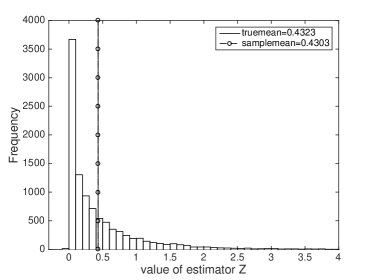
Figure 1: Histogram of Estimator $Z$ when $\alpha=1$

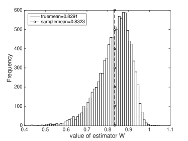
(a) Histogram of Estimator $W$

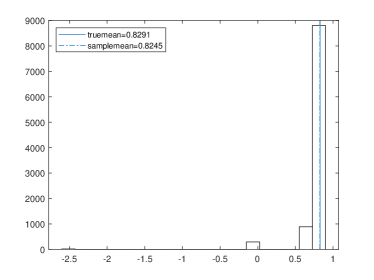
(b) Estimators based on Numerical PDE

Figure 2: Comparsion of Multilevel Estimators based on Antithetic Numerical SDE or Numerical PDE

Example 2

In this example, we consider the more complicated SDE:

$$\begin{cases}dX_{t}&=-\bm{\mu}(X_{t})dt+\cos(X_{t})dB_{t}\qquad\text{for $t\geq 0$}\\ X_{0}&=0,\end{cases}$$ (4.3)

where $\bm{\mu}(x)=\sum\limits_{i=1}^{\infty}i^{-4}\sin(ix)\bm{V}_{i}$ and we compare the proposed method with the standard Monte Carlo method with bias. We take $\gamma=\frac{1}{3}$ and $\theta=\frac{4}{3}$ for simplicity ( the detailed discussion in Section A). Similar to the previous example, we take $n_{0}=n_{1}=5$. We generate $10,000$ copies of our estimator and compare it with $10,000$ copies of a standard Monte Carlo estimator where we remove the debiasing part $\frac{\Delta_{N}}{p_{N}}$ in both estimator $Z$ and $W$. As a result, using the CLT, we compute a 95% confidence interval $[0.4610,0.4656]$ for our estimator while we obtain an interval $[0.5189,0.5255]$ for the standard Monte Carlo estimator. As we can see, these two intervals are not overlapping, suggesting that the standard Monte Carlo estimator has shown a significant bias.

Appendix A Proofs

In this section, we present the proofs for Lemma 3.2.4, Lemma 3.2.8 and Lemma 2.1.2. The proof for all the supporting lemmas are provided in the Appendix.

A.1 Definitions and supporting lemmas

To prove Lemma 3.2.4, we introduce several definitions and supporting lemmas.

Definition A.1.1.

Let $\epsilon$ to be a positive constant small enough to satisfy

$$\epsilon<\frac{1}{144}\ \ \ \ \text{and}\ \ \ \ \epsilon<\frac{1}{36}(\frac{1}{6}-12\epsilon)(q-4),$$ (A.1)

where $q>4$ is from Assumption 1, so that we can define positive quantities

$$\alpha\triangleq\frac{1}{2}-\epsilon,\ \ \beta\triangleq\frac{1}{2}+2\epsilon,\ \ \gamma\triangleq\frac{1}{3}-12\epsilon,\ \ \ \theta\triangleq\frac{4}{3}-\frac{23}{2}\epsilon\ \ \ and\ \ \ \delta\triangleq 33\epsilon$$ (A.2)

It is easy to check that the following important inequalities are satisfied :

$$\gamma\geq \frac{1}{4},\quad(3+\frac{q-4}{2})\gamma>1,\quad 8(2\alpha-\beta)>4-\delta>0,$$

$$4-\delta> 3\theta>0\quad(\text{as in Lemma\leavevmode\nobreak\ \ref{finitefourthmoment2}})\quad\text{and}\quad\theta>1+\gamma>0\quad(\text{as in Lemma\leavevmode\nobreak\ \ref{computecost}}).$$ (A.3)

Definition A.1.2.

For a standard one-dimensional Brownian motion $B(t)$ on $[0.1]$, let $\alpha$ and $\beta$ be defined as in Definition A.1.1. Then, define

$$\|B\|_{\alpha}\triangleq\sup_{0\leq s<t\leq 1}\frac{\|B(t)-B(s)\|_{\infty}}{\lvert t-s\rvert^{\alpha}}\qquad\text{and}\qquad\|A\|_{2\alpha}\triangleq\sup_{0\leq s<t\leq 1}\max_{1\leq i,j\leq d^{\prime}}\frac{\lvert A_{i,j}(s,t)\rvert}{\lvert t-s\rvert^{2\alpha}}$$ (A.4)

$$\|\tilde{A}\|_{2\alpha}\triangleq\sup_{0\leq s\leq t\leq 1}\max_{1\leq i,j\leq d^{\prime}}\frac{\lvert\widetilde{A}_{i,j}(s,t)\rvert}{\lvert t-s\rvert^{2\alpha}}\qquad\text{and}\qquad\Gamma_{\widetilde{R}}\triangleq\sup_{n}\sup_{\begin{subarray}{c}0\leq s\leq t\leq 1\\ s,t\in D_{n}\end{subarray}}\max_{1\leq i,j\leq d^{\prime}}\frac{\lvert\widetilde{R}_{i,j}^{n}(s,t)\rvert}{\lvert t-s\rvert^{\beta}\Delta t_{n}^{2\alpha-\beta}},$$ (A.5)

where $D_{n}$ is the dyadic rationals that are multiples of $\frac{1}{2^{n}}$ in $[0,1]$, and for $1\leq i,j\leq d^{\prime},i\neq j$,

$$A_{i,j}(s,t)\triangleq\int_{s}^{t}(B_{i}(u)-B_{i}(s))dB_{j}(u)\leavevmode\nobreak\ \leavevmode\nobreak\ \text{and}\leavevmode\nobreak\ \leavevmode\nobreak\ \widetilde{A}_{i,i}(s,t)\triangleq{A}_{i,i}(s,t)=\frac{(B_{i}(t)-B_{i}(s))^{2}-(t-s)}{2},$$ (A.6)

$$\widetilde{A}_{i,j}(s,t)\triangleq\frac{(B_{i}(t)-B_{i}(s))(B_{j}(t)-B_{j}(s))}{2}\leavevmode\nobreak\ \leavevmode\nobreak\ \text{and}\leavevmode\nobreak\ \leavevmode\nobreak\ \widetilde{R}_{i,j}^{n}(t_{l}^{n},t_{m}^{n})\triangleq\sum_{k=l+1}^{m}\{A_{i,j}(t_{k-1}^{n},t_{k}^{n})-\widetilde{A}_{i,j}(t_{k-1}^{n},t_{k}^{n})\},$$ (A.7)

some of which we have already defined in Definition 3.2.1.

Definition A.1.3 (Notation).

Throughout the proof section, we will use $C$ to represent any constant greater than 1 (i.e., $C>1$) and use $\mathcal{P}(\cdot)$ to represent any polynomial function from $\mathbb{R}^{n}\rightarrow\mathbb{R}$ where $n\geq 1$ such that $\mathcal{P}({x})>1$ for any ${x}_{1}>1$, $x_{i}\geq 0$ for $2\leq i\leq n$, and $x=(x_{1},...,x_{n})$. We will simply write this as $\mathcal{P}(x)>1$ for $x>1$ and it will not affect our analysis.

It is straightforward to verify that for any $\mathcal{P}_{1}(\cdot),\mathcal{P}_{2}(\cdot)$ and $n\geq 0$, we can find some $\mathcal{P}_{3}(x)$ that

$$(\mathcal{P}_{1}(x))^{n}< \mathcal{P}_{3}(x)$$

$$\mathcal{P}_{1}(x)+\mathcal{P}_{2}(x)< \mathcal{P}_{3}(x)$$

$$\mathcal{P}_{1}(x)\cdot\mathcal{P}_{2}(x)< \mathcal{P}_{3}(x)$$

$$\mathcal{P}_{2}(\mathcal{P}_{1}(x))< \mathcal{P}_{3}(x).$$ (A.8)

Lemma A.1.4 (Supporting Lemma).

The quantities $\|B\|_{\alpha},\|A\|_{2\alpha}$, $\|\tilde{A}\|_{2\alpha}$ and $\Gamma_{\widetilde{R}}$ defined in Definition A.1.2 have moments of arbitrary order.

Lemma A.1.5 (Supporting Lemma).

Let $X_{n}(\cdot)$ be the discretization scheme in Definition 3.2.2 generated under $\mu^{(n)}(\cdot)\in\mathcal{L}_{1}$ with the bounding number $L_{1}>1$ and Brownian motion $B(t),0\leq t\leq 1$. Then, we can find some fixed polynomial function $\mathcal{P}(x)>1$ for $x>1$ $:\mathbb{R}^{3}\rightarrow\mathbb{R}$ such that

$$\|X_{n}(t)-X_{n}(r)\|_{\infty}\leq\mathcal{P}(L_{1},\|B\|_{\alpha},\|\widetilde{A}\|_{2\alpha})\lvert t-r\rvert^{\alpha}$$

for $0\leq r\leq t\leq 1$ and for all $n\geq 0$.

Lemma A.1.6 (Supporting Lemma).

Let $X^{\mu}_{n}(\cdot)$ be the discretization scheme modified from Definition 3.2.2 generated under $\mu(\cdot)\in\mathcal{L}_{1}$ (instead of $\mu^{n}(\cdot)$) with the bounding number $L_{1}>1$ and Brownian motion $B(t),0\leq t\leq 1$. Also, let $X_{t},0\leq t\leq 1$ be the solution of SDE in (3.2). Then, we can find some fixed polynomial $\mathcal{P}(x)>1$ for $x>1$$:\mathbb{R}^{4}\rightarrow\mathbb{R}$ such that

$$\|X_{n}^{\mu}(t)-X_{t}\|_{\infty}\leq\mathcal{P}(L_{1},\|B\|_{\alpha},\|A\|_{2\alpha},\Gamma_{\widetilde{R}})\Delta t_{n}^{2\alpha-\beta}$$ (A.9)

for all $n\geq 0$ and $0\leq t\leq 1$.

Lemma A.1.7 (Supporting Lemma).

Let $X_{n+1}(1)$ and $X^{a}_{n+1}(1)$ be defined as in Definition 3.2.1 and 3.2.2 generated under fixed $\mu^{(n+1)}(\cdot)\in\mathcal{L}_{1}$ with the bounding number $L_{1}>1$. Then, we can find some fixed polynomial $\mathcal{P}(x)>1$ for $x>1$ such that

$$\mathbb{E}[\|X_{n+1}(1)-X_{n+1}^{a}(1)\|_{\infty}^{8}]\leq\mathcal{P}(L_{1})\Delta t_{n}^{8(2\alpha-\beta)}.$$ (A.10)

A.2 Proof of Lemma 3.2.4

Proof of Lemma  3.2.4.

Let $X_{t},0\leq t\leq 1$ be the solution of the SDE under $\mu(\cdot)\in\mathcal{L}_{1}$ with the bounding number $L_{1}>1$ and $X_{n}(t)$ be the discretization scheme in Definition 3.2.2 generated under $\mu^{(n)}(\cdot)\in\mathcal{L}_{1}$ with the bounding number $L_{1}>1$. Additionally, let $X^{\mu}_{n}(\cdot)$ be the discretization scheme modified from Definition 3.2.2 generated under $\mu(\cdot)\in\mathcal{L}_{1}$ with the bounding number $L_{1}>1$ instead of $\mu^{n}(\cdot)$. Then, for $0\leq t\leq 1$, we have the following bound on $\|X_{n}(t)-X_{t}\|_{\infty}$,

$$\|X_{n}(t)-X_{t}\|_{\infty}\leq\|X_{n}(t)-X_{n}^{\mu}(t)\|_{\infty}+\|X_{n}^{\mu}(t)-X_{t}\|_{\infty}.$$ (A.11)

In order to prove Lemma 3.2.4, we provide bounds for both $\|X_{n}(t)-X_{n}^{\mu}(t)\|_{\infty}$ and $\|X_{n}^{\mu}(t)-X_{t}\|_{\infty}$.

For $\|X_{n}^{\mu}(t)-X_{t}\|_{\infty}$, using Lemma A.1.6, we can find a polynomial $\mathcal{P}(x)>1$ for $x>1$ such that

$$\|X_{n}^{\mu}(t)-X_{t}\|_{\infty}\leq\mathcal{P}(L_{1},\|B\|_{\alpha},\|A\|_{2\alpha},\Gamma_{\widetilde{R}})\Delta t_{n}^{2\alpha-\beta}.$$ (A.12)

Similarly, using Lemma A.1.3, we can further find some polynomial $\mathcal{P}(x)>1$ for $x>1$ such that

$$\|X_{n}^{\mu}(t)-X_{t}\|^{4}_{\infty}\leq\mathcal{P}(L_{1},\|B\|_{\alpha},\|A\|_{2\alpha},\Gamma_{\widetilde{R}})\Delta t_{n}^{4(2\alpha-\beta)}.$$ (A.13)

It follows from Lemma A.1.4 that the quantities associated with Brownian motions $\|B\|_{\alpha}$,$\|A\|_{2\alpha}$ and $\Gamma_{\widetilde{R}}$ have moments of arbitrary order. Thus, fixing $\mu(\cdot)\in\mathcal{L}_{1}$, we can find some polynomial $\mathcal{P}^{\prime}(x)>1$ for $x>1$ such that

$$\mathbb{E}\|X^{\mu}_{n}(t)-X_{t}\|_{\infty}^{4}\leq \mathbb{E}[\mathcal{P}(L_{1},\|B\|_{\alpha},\|A\|_{2\alpha},\Gamma_{\widetilde{R}})]\Delta t_{n}^{4(2\alpha-\beta)}$$

$$\leq \mathcal{P}^{\prime}(L_{1})\Delta t_{n}^{4(2\alpha-\beta)}$$

$$\leq e^{CL_{1}}\Delta t_{n}^{4(2\alpha-\beta)},$$ (A.14)

for some constant $C>1$ since $L_{1}>1$. Combining this with (A.11), we have

$$\mathbb{E}\|X_{n}(t)-X_{t}\|^{4}_{\infty}\leq 8\mathbb{E}\|X_{n}(t)-X_{n}^{\mu}(t)\|^{4}_{\infty}+8e^{CL_{1}}\Delta t_{n}^{4(2\alpha-\beta)}.$$ (A.15)

Thus, we can complete the proof if we can show

$$\mathbb{E}\|X_{n}(t)-X_{n}^{\mu}(t)\|^{4}_{\infty}\leq e^{CL_{1}}\Delta t_{n}^{4\alpha},$$ (A.16)

for some $C>1$. This is because we have, according to Lemma A.1.1,

$$4\alpha=2-4\epsilon>2-16\epsilon=4(2\alpha-\beta)$$ (A.17)

and thus (A.16) would imply

$$\mathbb{E}\|X_{n}(t)-X_{n}^{\mu}(t)\|^{4}_{\infty}\leq e^{CL_{1}}\Delta t_{n}^{4(2\alpha-\beta)},$$ (A.18)

since $\Delta t_{n}<1$. Finally, we can simply conclude the proof using (A.15) and (A.18) by adjusting the constant $C$. To prove (A.16), we define

$$\bar{\mu}^{(n)}(\cdot)\triangleq\mu-\mu^{(n)}=\sum_{i=\lfloor 2^{n\gamma}\rfloor+1}^{\infty}\frac{\lambda_{i}}{i^{q}}V_{i}(\omega)\psi_{i}(\cdot)$$ (A.19)

to be the remaining sum when we approximate $\mu$ by $\mu^{(n)}$. In Section A.4 of the proof of Lemma 2.1.2, we will show that

$$\|\bar{\mu}^{(n)}(\cdot)\|_{\infty}\leq L_{1}\Delta t_{n}^{3+\frac{q-4}{2}}.$$ (A.20)

Then, we may conduct the analysis on $\|X_{n}(t)-X_{n}^{\mu^{(n)}}(t)\|_{\infty}$ based on the following recursion: for $1\leq i\leq d$, $0\leq k\leq 2^{n}-1$,

$$X_{i,n}^{\mu}(t_{k+1}^{n})-X_{i,n}(t_{k+1}^{n})$$

$$= X_{i,n}^{\mu}(t_{k}^{n})-X_{i,n}(t_{k}^{n})+\Big{(}\mu_{i}^{(n)}(X^{\mu}_{n}(t_{k}^{n}))-\mu_{i}^{(n)}(X_{n}(t_{k}^{n}))\Big{)}\Delta t_{n}+\bar{\mu}^{(n)}(X_{n}^{\mu}(t_{k}^{n}))\Delta t_{n}$$

$$+\sum_{j=1}^{d}\sigma_{ij}(X_{n}^{\mu}(t_{k}^{n}))-\sigma_{ij}(X_{n}(t_{k}^{n}))\Delta B_{j,k}^{n}$$

$$+\sum_{j=1}^{d^{\prime}}\sum_{l=1}^{d}\sum_{m=1}^{d^{\prime}}\Big{(}\frac{\partial\sigma_{ij}}{\partial x_{l}}(X_{n}^{\mu}(t_{k}^{n}))\sigma_{lm}(X_{n}^{\mu}(t_{k}^{n}))-\frac{\partial\sigma_{ij}}{\partial x_{l}}(X_{n}(t_{k}^{n}))\sigma_{lm}(X_{n}(t_{k}^{n}))\Big{)}\widetilde{A}_{mj}(t_{k}^{n},t_{k+1}^{n}),$$ (A.21)

which is obtained by modifying (3.2.2) and simply taking the difference. Now, let

$$\xi_{n,k}\triangleq X_{n}^{\mu}(t_{k}^{n})-X_{n}(t_{k}^{n})\qquad\text{and}\qquad\xi_{i,n,k}\triangleq X_{i,n}^{\mu}(t_{k}^{n})-X_{i,n}(t_{k}^{n})$$ (A.22)

for $1\leq i\leq d$ and $0\leq k\leq 2^{n}$ and let

$$\eta_{i,n,k}\triangleq \big{(}\mu_{i}^{(n)}(X^{\mu}_{n}(t_{k}^{n}))-\mu_{i}^{(n)}(X_{n}(t_{k}^{n}))\big{)}\Delta t_{n}+\bar{\mu}^{(n)}(X_{n}^{\mu}(t_{k}^{n}))\Delta t_{n}$$

$$+\sum_{j=1}^{d}\Big{(}\sigma_{ij}(X_{n}^{\mu}(t_{k}^{n}))-\sigma_{ij}(X_{n}(t_{k}^{n}))\Big{)}\Delta B_{j,k}^{n}$$

$$+\sum_{j=1}^{d^{\prime}}\sum_{l=1}^{d}\sum_{m=1}^{d^{\prime}}\Big{(}\frac{\partial\sigma_{ij}}{\partial x_{l}}(X_{n}^{\mu}(t_{k}^{n}))\sigma_{lm}(X_{n}^{\mu}(t_{k}^{n}))-\frac{\partial\sigma_{ij}}{\partial x_{l}}(X_{n}(t_{k}^{n}))\sigma_{lm}(X_{n}(t_{k}^{n}))\Big{)}\widetilde{A}_{mj}(t_{k}^{n},t_{k+1}^{n}),$$ (A.23)

so that (A.2) becomes, for $1\leq i\leq d$, $0\leq k\leq 2^{n}-1$,

$$\xi_{i,n,k+1}=\xi_{i,n,k}+\eta_{i,n,k}.$$ (A.24)

Fixing ${\mu}\in\mathcal{L}_{1}$ and $\mu^{(n)}\in\mathcal{L}_{1}$ with bounding number $L_{1}>1$ and taking expectation on (A.24) after raising it to the fourth power, we have

$$\mathbb{E}(\xi_{i,n,k+1}^{4})= \mathbb{E}(\xi_{i,n,k}^{4})+\mathbb{E}_{\mu(\omega)}(\eta_{i,n,k}^{4})+3\mathbb{E}(\xi_{i,n,k}^{3}\eta_{i,n,k})+3\mathbb{E}(\xi_{i,n,k}\eta_{i,n,k}^{3})+6\mathbb{E}(\xi_{i,n,k}^{2}\eta_{i,n,k}^{2}).$$ (A.25)

It now follows from the definition of $\xi_{i,n,k}$ in (A.22) that it is sufficient to show

$$\mathbb{E}\|X_{n}(t)-X_{n}^{\mu}(t)\|^{4}_{\infty}=\mathbb{E}\|\xi_{n,2^{n}}\|_{\infty}^{4}\leq e^{CL_{1}}\Delta t_{n}^{4\alpha},$$ (A.26)

for some constant $C>1$. Thus, in what follows, we focus on the proof of (A.26), which consists of proofs for the following two statements: fixing ${\mu}\in\mathcal{L}_{1}$ and $\mu^{(n)}\in\mathcal{L}_{1}$ with bounding number $L_{1}>1$,

• (I) We prove that there exists a constant $C>1$ and a polynomial $\mathcal{P}(x)>1$ for $x>1$ such that for $1\leq i\leq d$ and $0\leq k\leq 2^{n}$, we have

  $$\mathbb{E}\lvert\xi_{i,n,k}\rvert^{4}\leq e^{CL_{1}\cdot t_{k}^{n}}\Delta t_{n}^{4\alpha}$$ (A.27)

  if $n$ is large enough so that $2^{n}>\mathcal{P}(L_{1})$.

• (II) We prove that there is a polynomial $\mathcal{P}^{\prime}(x)>1$ for $x>1$ such that for $1\leq i\leq d$ and $0\leq k\leq 2^{n}$, we have

  $$\mathbb{E}\lvert\xi_{i,n,k}\rvert^{4}\leq\mathcal{P}^{\prime}(L_{1})\Delta t_{n}^{4\alpha},$$ (A.28)

  if $n$ is not large enough and $2^{n}\leq\mathcal{P}(L_{1})$.

Proof of statement (I)

Fixing ${\mu}\in\mathcal{L}_{1}$ and $\mu^{(n)}\in\mathcal{L}_{1}$ with bounding number $L_{1}>1$, we use induction on $0\leq k\leq 2^{n}$. First of all, when $k=0$, for $1\leq i\leq d$, the claim holds since $\xi_{i,n,0}=X_{i,n}^{\mu}(0)-X_{i,n}(0)=x-x=0$.

Next, for $0<k\leq 2^{n}-1$ , assume that the induction hypothesis holds so that whenever $0\leq j\leq k$,

$$\mathbb{E}\lvert\xi^{4}_{i,n,j}\rvert\leq e^{CL_{1}t_{j}^{n}}\cdot\Delta t_{n}^{4\alpha}$$ (A.29)

for $1\leq i\leq d$ and some $C>1$. Our goal is to show

$$\mathbb{E}\lvert\xi^{4}_{i,n,k+1}\rvert\leq e^{CL_{1}t_{k+1}^{n}}\cdot\Delta t_{n}^{4\alpha}$$ (A.30)

for all $1\leq i\leq d$. To do this, we provide bounds for every term on the right hand side of (A.25). For $\eta^{4}_{i,n,k}$, according to Definition A.1.2 and denoting $\bar{d}=\max\{d,d^{\prime}\}$, we have

$$\lvert\eta_{i,n,k}\rvert\leq \|\partial{\mu_{i}^{(n)}}\|_{\infty}\|\xi_{n,k}\|_{\infty}\Delta t_{n}+\|\bar{\mu}^{(n)}\|_{\infty}\Delta t_{n}+\bar{d}L\|\xi_{n,k}\|_{\infty}\|B\|_{\alpha}\Delta t_{n}^{\alpha}$$

$$+{\bar{d}}^{3}L\|\xi_{n,k}\|_{\infty}\|A\|_{2\alpha}\Delta t_{n}^{2\alpha}$$

$$\leq L_{1}\|\xi_{n,k}\|_{\infty}\Delta t_{n}+L_{1}\Delta t_{n}^{4+\frac{q-4}{2}}+\bar{d}L\|\xi_{n,k}\|_{\infty}\|B\|_{\alpha}\Delta t_{n}^{\alpha}$$

$$+{\bar{d}}^{3}L\|\xi_{n,k}\|_{\infty}\|A\|_{2\alpha}\Delta t_{n}^{2\alpha}$$ (A.31)

where the last line follows from (A.20). Since $\xi_{n,k}$ and the shifted Brownian motion on $B(t)-B(t_{k}^{n}),t_{k}^{n}\leq t\leq t_{k+1}^{n}$ are independent of each other (i.e., independent increments of Brownian motion), we can consider quantities $\|B\|_{\alpha}$ and $\|A\|_{2\alpha}$ to be associated with the new Brownian motion $B(t)-B(t_{k}^{n}),t_{k}^{n}\leq t\leq t_{k+1}^{n}$ and thus independent of $\xi_{n,k}$. Consequently, it then follows from Lemma  A.1.4 that we can find a constant $C^{\prime}>1$ such that

$$\mathbb{E}\eta_{i,n,k}^{4} \leq C^{\prime}\bigg{(}L_{1}^{4}\mathbb{E}(\|\xi_{n,k}\|_{\infty}^{4})\Delta t_{n}^{4}+L_{1}^{4}\Delta t_{n}^{16+2(q-4)}+\mathbb{E}(\|\xi_{n,k}\|_{\infty}^{4})\Delta t_{n}^{4\alpha}+\mathbb{E}(\|\xi_{n,k}\|_{\infty}^{4})\Delta t_{n}^{8\alpha}\bigg{)}$$

$$\leq C^{\prime\prime}L_{1}^{4}\bar{d}^{4}e^{CL_{1}\cdot t_{k}^{n}}\cdot\Delta t_{n}^{8\alpha}$$ (A.32)

for some $C^{\prime\prime}>1$ where the last line follows from both the induction hypothesis and the fact that $8\alpha<16+2(q-4)$ in Definition A.1.1.

For the bound on $\mathbb{E}(\xi_{i,n,k}^{3}\eta_{i,n,k})$ in (A.25), we observe the terms in (A.2) and use (A.20) along with the martingale property (i.e., the independence of $\Delta B_{k}^{n}$ and $X_{n}(t_{k}^{n})$) to obtain

$$\mathbb{E}(\xi_{i,n,k}^{3}\eta_{i,n,k})$$

$$= \mathbb{E}\big{[}\big{(}X_{i,n}^{\mu}(t_{k}^{n})-X_{i,n}^{\mu^{(n)}}(t_{k}^{n})\big{)}^{3}\cdot\Big{(}\big{(}\mu_{i}^{(n)}(X^{\mu}_{n}(t_{k}^{n}))-\mu_{i}^{(n)}(X^{\mu^{(n)}}_{n}(t_{k}^{n}))\big{)}\Delta t_{n}+\bar{\mu}^{(n)}(X_{n}^{\mu}(t_{k}^{n}))\Delta t_{n}\Big{)}\big{]}$$

$$\leq \mathbb{E}[L_{1}\|\xi_{n,k}\|_{\infty}^{4}\Delta t_{n}]+\mathbb{E}[L_{1}\|\xi_{n,k}\|_{\infty}^{3}\Delta t_{n}^{4+\frac{q-4}{2}}]$$

$$\leq \bigg{(}\mathbb{E}(\|\xi_{n,k}\|_{\infty}^{4})+\mathbb{E}(\|\xi_{n,k}\|_{\infty}^{4})^{\frac{3}{4}}\Delta t_{n}^{\alpha}\bigg{)}L_{1}\Delta t_{n}\leq 2L_{1}\bar{d}^{4}e^{CL_{1}\cdot t_{k}^{n}}\Delta t_{n}^{4\alpha+1}.$$

The last inequality follows from induction hypothesis, the second inequality follows from Hölder’s inequality and the fact that $\alpha<4+\frac{q-4}{2}$ as in Definition A.1.1, and the first inequality follows from the bound on $\|\partial{\mu_{i}^{(n)}}\|_{\infty}$ in Assumption 1.

For the bound on $\mathbb{E}(\xi_{i,n,k}^{2}\eta_{i,n,k}^{2})$, using the bound on $\lvert\eta_{i,n,k}\rvert$ in (A.2) and the fact that $\mathbb{E}[\big{(}B(t)-B(s)\big{)}^{2}]=O(|t-s|)$ and $\mathbb{E}[\big{(}\widetilde{A}_{ij}(s,t)\big{)}^{2}]=O((t-s)^{2})$ (see, for example, [20]), we can find some $C^{\prime}>1$ that

$$\mathbb{E}(\xi_{i,n,k}^{2}\eta_{i,n,k}^{2})\leq C^{\prime}\Big{(}\mathbb{E}({\|\xi_{n,k}\|_{\infty}^{4}})L_{1}^{2}\Delta t_{n}^{2}+\mathbb{E}({\|\xi_{n,k}\|_{\infty}^{2}})L_{1}^{2}\Delta t_{n}^{4+q}$$ (A.34)

$$+\mathbb{E}({\|\xi_{n,k}\|_{\infty}^{4}})\Delta t_{n}+\mathbb{E}({\|\xi_{n,k}\|_{\infty}^{4}}){\Delta t_{n}^{2}}\Big{)}$$

$$\leq C^{\prime}\mathbb{E}(\|\xi_{n,k}\|^{4}_{\infty})\Delta t_{n}\big{(}L_{1}^{2}\Delta t_{n}+2\big{)}+C^{\prime}\mathbb{E}(\|\xi_{n,k}\|^{4}_{\infty})^{\frac{1}{2}}\Delta t_{n}^{2\alpha+1}\big{(}L_{1}^{2}(\omega)\Delta t_{n}\big{)}$$

$$\leq 2C^{\prime\prime}\bar{d}^{4}e^{CL_{1}\cdot t_{k}^{n}}(L_{1}^{2}\Delta t_{n}+1)\Delta t_{n}^{4\alpha+1}$$ (A.35)

for some $C^{\prime\prime}>1$. The last line follows from induction hypothesis. The second to last line follows from Hölder’s inequality and the fact that $2\alpha+2<4+q$ as in Definition A.1.1. Finally, to bound $\mathbb{E}(\xi_{i,n,k}\eta_{i,n,k}^{3})$ in (A.25), following similar techniques, we use inequality (A.2), induction hypothesis and Hölder’s inequality to obtain

$$\mathbb{E}(\xi_{i,n,k}\eta_{i,n,k}^{3})\leq (\mathbb{E}(\xi_{i,n,k}^{4}))^{\frac{1}{4}}(\mathbb{E}(\eta_{i,n,k}^{4}))^{\frac{3}{4}}\leq C^{\prime\prime}L_{1}^{3}\bar{d}^{3}e^{CL_{1}\cdot t_{k}^{n}}\Delta t_{n}^{7\alpha}.$$ (A.36)

Now we are ready to prove the induction hypothesis. Let

$$C=12C^{\prime\prime}\bar{d}^{4}+6\bar{d}^{4}+1\quad\text{and}\quad\mathcal{P}(x)=\bigg{(}C^{\prime\prime}(x^{4}\bar{d}^{4}+3x^{3}\bar{d}^{3}+12x^{2}\bar{d}^{4})\bigg{)}^{3}.$$ (A.37)

It is easy to check that $C>1$ and the polynomial $\mathcal{P}(x)>1$ for $x>1$. Then, it follows from Definition A.1.1 and standard calculation that if $n$ is large enough that $2^{n}>\mathcal{P}(L_{1})$(i.e., $\Delta t_{n}<(\mathcal{P}(L_{1}))^{-1}$), then

$$C^{\prime\prime}L_{1}^{4}\bar{d}^{4}\Delta t_{n}^{4\alpha-1}+3C^{\prime\prime}L_{1}^{3}\bar{d}^{3}\Delta t_{n}^{3\alpha-1}+12C^{\prime\prime}L_{1}^{2}\bar{d}^{4}\Delta t_{n}$$

$$\leq (C^{\prime\prime}L_{1}^{4}\bar{d}^{4}+3C^{\prime\prime}L_{1}^{3}\bar{d}^{3}+12C^{\prime\prime}L_{1}^{2}\bar{d}^{4})\Delta t_{n}^{3\alpha-1}$$

$$= (\mathcal{P}(L_{1}))^{\frac{1}{3}}\Delta t_{n}^{3\alpha-1}<(\mathcal{P}(L_{1}))^{\frac{4}{3}-3\alpha}<1$$ (A.38)

where the last inequality follows from the fact that $0>\frac{4}{3}-3\alpha$, $L_{1}>1$ and $\mathcal{P}(x)>1$ for $x>1$. Thus, for $n$ such that $2^{n}>\mathcal{P}(L_{1})$, we use (A.25), Hölder’s inequality and the bound acquired in (A.2), (A.2), (A.34) and (A.36) to get

$$\mathbb{E}(\xi_{i,n,k+1}^{4})= \mathbb{E}(\xi_{i,n,k}^{4})+\mathbb{E}_{\mu(\omega)}(\eta_{i,n,k}^{4})+3\mathbb{E}(\xi_{i,n,k}^{3}\eta_{i,n,k})+3\mathbb{E}(\xi_{i,n,k}\eta_{i,n,k}^{3})+6\mathbb{E}(\xi_{i,n,k}^{2}\eta_{i,n,k}^{2})$$

$$\leq e^{CL_{1}\cdot t_{k}^{n}}\Delta t_{n}^{4\alpha}\big{(}1+C^{\prime\prime}L_{1}^{4}\bar{d}^{4}\Delta t_{n}^{4\alpha}+6L_{1}\bar{d}^{4}\Delta t_{n}+3C^{\prime\prime}L_{1}^{3}\bar{d}^{3}\Delta t_{n}^{3\alpha}+12C^{\prime\prime}\bar{d}^{4}(L_{1}^{2}\Delta t_{n}+1)\Delta t_{n}\big{)}$$

$$\leq e^{CL_{1}t_{k}^{n}}\Delta t_{n}^{4\alpha}\big{(}1+(6\bar{d}^{4}+12C^{\prime\prime}\bar{d}^{4}+1)L_{1}\Delta t_{n}\big{)}$$

$$= e^{CL_{1}t_{k}^{n}}\Delta t_{n}^{4\alpha}(1+CL_{1}\Delta t_{n})\leq e^{CL_{1}t_{k+1}^{n}}\Delta t_{n}^{4\alpha}$$ (A.39)

where the last line follows from convexity of exponential function: $e^{y}\geq e^{x}+e^{x}\cdot(y-x)$ for $y\geq x$. The second to last inequality follows from (A.37), (A.2) and the fact that $L_{1}>1$. This concludes the induction. However, since $t_{n}^{k}\leq 1$ for all $0\leq k\leq 2^{n}$, we have actually proven that when $2^{n}>\mathcal{P}(L_{1})$(i.e., $\Delta t_{n}<(\mathcal{P}(L_{1}))^{-1}$),

$$\mathbb{E}\|X^{\mu}_{i,n}(t)-X_{i,n}(t)\|_{\infty}^{4}\leq e^{CL_{1}}\cdot\Delta t_{n}^{4\alpha}$$ (A.40)

for all $1\leq i\leq d$ and $0\leq t\leq 1$.

Proof of statement (II)

Next, we extend the result to the case where $2^{n}\leq\mathcal{P}(L_{1})$. By observing (A.2), we can find polynomial function $\mathcal{P}^{\prime}(x)>1$ for $x>1$ so that:

$$\lvert({X_{i,n}^{\mu}(t_{k+1}^{n})-X_{i,n}(t_{k+1}^{n})})-({X_{i,n}^{\mu}(t_{k}^{n})-X_{i,n}(t_{k}^{n})})\rvert\leq\mathcal{P}^{\prime}(L_{1},\|B\|_{\alpha},\|\widetilde{A}\|_{2\alpha})\Delta t_{n}^{\alpha}.$$ (A.41)

Since the number of iterations in the discretization scheme $2^{n}$ is at most ${\mathcal{P}(L_{1})}$, we have

$$\|X_{i,n}^{\mu}(\cdot)-X_{i,n}(\cdot)\|_{\infty}\leq{\mathcal{P}(L_{1})}\mathcal{P}^{\prime}(L_{1},\|B\|_{\alpha},\|\widetilde{A}\|_{2\alpha})\Delta t_{n}^{\alpha},$$ (A.42)

and consequently, from Lemma A.1.4, that

$$\mathbb{E}\|X_{i,n}^{\mu}(\cdot)-X_{i,n}(\cdot)\|_{\infty}^{4}\leq\mathcal{P}^{\prime\prime}(L_{1})\Delta t_{n}^{4\alpha}$$ (A.43)

for some polynomial $\mathcal{P}^{\prime\prime}(x)>1$ when $x>1$.

This concludes the proof of Lemma 3.2.4. ∎

A.3 Proof of Lemma 3.2.8

We first prove the second claim (3.18) of Lemma 3.2.8:

Proof of (3.18) in Lemma 3.2.8.

Assume without loss of generality that $x=0$. Fixing ${\mu}\in\mathcal{L}_{1}$ and $\mu^{(n)}\in\mathcal{L}_{1}$ with bounding number $L_{1}>1$, since

$$\sup_{1\leq k\leq 2^{n}}\lvert X_{i,n}(t_{k}^{n})\rvert^{4}\leq \Big{(}\sum_{k=0}^{2^{n}}\|\mu\|_{\infty}\Delta t_{n}+\sum_{j}\sup_{1\leq h\leq 2^{n}}|\sum_{k=0}^{h}\sigma_{ij}(X_{n}(t_{k}^{n}))\Delta B_{j,k}^{n}|$$

$$+\sum_{j,l,m}\sup_{1\leq h\leq 2^{n}}\lvert\sum_{k=0}^{h}\frac{\partial\sigma_{ij}}{\partial x_{l}}(X_{n}(t_{k}^{n}))\sigma_{lm}(X_{n}(t_{k}^{n}))\widetilde{A}_{mj}(t_{k}^{n},t_{k+1}^{n})\rvert\Big{)},$$ (A.44)

it follows from (3.2.2) and Assumption 1 that we can find constant $C>1$ such that

$$\sup_{1\leq k\leq 2^{n}}\lvert X_{i,n}(t_{k}^{n})\rvert^{4}\leq C\cdot\Big{(}L_{1}^{4}+\sum_{j}\big{(}\sup_{1\leq h\leq 2^{n}}|\sum_{k=0}^{h}\sigma_{ij}(X_{n}(t_{k}^{n}))\Delta B_{j,k}^{n}|\big{)}^{4}$$

$$+\sum_{j,l,m}\big{(}\sup_{1\leq h\leq 2^{n}}\lvert\sum_{k=0}^{h}\frac{\partial\sigma_{ij}}{\partial x_{l}}(X_{n}(t_{k}^{n}))\sigma_{lm}(X_{n}(t_{k}^{n}))\widetilde{A}_{mj}(t_{k}^{n},t_{k+1}^{n})\rvert\big{)}^{4}\Big{)}.$$ (A.45)

Now, using the fact that $\mathbb{E}\big{(}B(t)-B(s)\big{)}^{4}=O(t-s)^{2}$ and $\mathbb{E}\big{(}\widetilde{A}_{ij}(s,t)\big{)}^{4}=O(t-s)^{4}$, we recall Burkholder-Davis-Gundy inequality [5] to further find constant $C^{\prime}>1$ and $C^{\prime\prime}>1$ so that

$$\mathbb{E}\sup_{1\leq k\leq 2^{n}}\lvert X_{i,n}(t_{k}^{n})\rvert^{4}\leq C\cdot\Big{(}L_{1}^{4}+\sum_{j}\sup_{1\leq h\leq 2^{n}}|\sum_{k=0}^{h}\sigma_{ij}(X_{n}(t_{k}^{n}))\Delta B_{j,k}^{n}|^{4}$$

$$+\sum_{j,l,m}\sup_{1\leq h\leq 2^{n}}\lvert\sum_{k=0}^{h}\frac{\partial\sigma_{ij}}{\partial x_{l}}(X_{n}(t_{k}^{n}))\sigma_{lm}(X_{n}(t_{k}^{n}))\widetilde{A}_{mj}(t_{k}^{n},t_{k+1}^{n})\rvert^{4}\Big{)}$$

$$\leq C^{\prime}\Big{(}L_{1}^{4}+\sum_{j}\mathbb{E}\big{(}\sum_{k=0}^{2^{n}}(\sigma_{ij}(X_{n}(t_{k}^{n})))^{2}(\Delta B_{j,k}^{n})^{2}\big{)}^{2}$$

$$+\sum_{j,l,m}\mathbb{E}\big{(}\sum_{k=0}^{2^{n}}(\frac{\partial\sigma_{ij}}{\partial x_{l}}(X_{n}(t_{k}^{n})))^{2}\sigma_{lm}^{2}(X_{n}(t_{k}^{n}))(\widetilde{A}_{mj}(t_{k}^{n},t_{k+1}^{n}))^{2}\big{)}^{2}\Big{)}$$

$$\leq C^{\prime}\Big{(}L_{1}^{4}+\sum_{j=1}^{d^{\prime}}\mathbb{E}2^{n}\sum_{k=0}^{2^{n}}(\sigma_{ij}(X_{n}(t_{k}^{n})))^{4}(\Delta B_{j,k}^{n})^{4}$$

$$+\sum_{j,l,m}\mathbb{E}2^{n}\sum_{k=0}^{2^{n}}(\frac{\partial\sigma_{ij}}{\partial x_{l}}(X_{n}(t_{k}^{n})))^{4}\sigma_{lm}^{4}(X_{n}(t_{k}^{n}))(\widetilde{A}_{mj}(t_{k}^{n},t_{k+1}^{n}))^{4}\Big{)}$$

$$\leq C^{\prime\prime}(L_{1}^{4}+L^{4}2^{n}(\sum_{k=0}^{2^{n}}\Delta t_{n}^{2}+\sum_{k=0}^{2^{n}}\Delta t_{n}^{4}))<\mathcal{P}(L_{1})$$ (A.46)

for some polynomial function $\mathcal{P}(x)>1$ for $x>1$. Now, the claim on $\mathbb{E}|f(X_{n_{0}}(1))|^{4}$ follows by invoking the bound on $\|\frac{\partial f}{\partial x_{i}}\|_{\infty}$ in Assumption  2. ∎

We proceed to the proof of the first claim of Lemma 3.2.8, namely (3.17).

Proof of (3.17) in Lemma 3.2.8.

It follows from Equation (3.20) in [16] that we have for $p\geq 2$

$$\lvert\Delta_{n}\rvert^{p}\leq 2^{p-1}L^{p}\mathbb{E}[\|\frac{1}{2}(X_{n+1}(1)+X_{n+1}^{a}(1))-X_{n}(1)\|_{\infty}^{p}]+2^{-p-1}L^{p}\mathbb{E}[\|X_{n+1}(1)-X_{n+1}^{a}(1)\|_{\infty}^{2p}].$$ (A.47)

Thus, according to (A.47), in order to prove Lemma 3.2.8,

$$\mathbb{E}(\Delta_{n}^{4})\leq e^{CL_{1}}\Delta t_{n}^{4-\delta},$$ (A.48)

where $\delta>0$ is defined in Definition A.1.1, it is sufficient to provide an upper bound on

$$\mathbb{E}[\|\frac{1}{2}(X_{n+1}(1)+X_{n+1}^{a}(1))-X_{n}(1)\|_{\infty}^{4}]$$ (A.49)

and

$$\mathbb{E}[\|X_{n+1}(1)-X_{n+1}^{a}(1)\|_{\infty}^{8}].$$ (A.50)

Note that bound on (A.50) is provided by Lemma A.1.7 since ${4-\delta}<{8(2\alpha-\beta)}$ as in Definition A.1.1 and $\mathcal{P}(L_{1})<e^{CL_{1}}$ for appropriately chosen $C>1$. So we just need to prove (A.49). First we write the recursion for $X_{n+1}(\cdot)$ over the coarse step $\Delta t_{n}$ instead of $\Delta t_{n+1}$. For $1\leq i\leq d$ and $1\leq k\leq 2^{n}$, adding up two steps of recursion for $X_{n+1}(\cdot)$, we have:

$$X_{i,n+1}(t_{k+1}^{n})=X {}_{i,n+1}(t_{k}^{n})+\mu_{i}^{(n+1)}(X_{n+1}^{f}(t_{k}^{n}))+\sum_{j=1}^{d^{\prime}}\sigma_{ij}(X_{n+1}(t_{k}^{n}))\Delta B_{j,k}^{n}$$

$$+\sum_{j=1}^{d^{\prime}}\sum_{l=1}^{d}\sum_{m=1}^{d^{\prime}}\frac{\partial\sigma_{ij}}{\partial x_{l}}(X_{n+1}(t_{k}^{n}))\sigma_{lm}(X_{n+1}(t_{k}^{n}))\widetilde{A}_{mj}(t_{k}^{n},t_{k+1}^{n})$$

$$-\sum_{j=1}^{d^{\prime}}\sum_{l=1}^{d}\sum_{m=1}^{d^{\prime}}\frac{\partial\sigma_{ij}}{\partial x_{l}}(X_{n+1}(t_{k}^{n}))\sigma_{lm}(X_{n+1}(t_{k}^{n}))(\Delta B_{j,2k}^{n+1}\Delta B_{m,2k+1}^{n+1}-\Delta B_{m,2k}^{n+1}\Delta B_{j,2k+1}^{n+1})$$

$$+N_{i,n,k}^{f}+M_{i,n,k}^{f,(1)}+M_{i,n,k}^{f,(2)}+M_{i,n,k}^{f,(3)}$$ (A.51)

where we define

$$M_{i,n,k}^{f,(2)}\triangleq \Big{(}\sum_{j=1}^{d^{\prime}}(\sigma_{ij}(X_{n+1}(t^{n+1}_{2k+1}))-\sigma_{ij}(X_{n+1}(t^{n}_{k})))-\sum_{j=1}^{d^{\prime}}\sum_{l=1}^{d}\sum_{m=1}^{d^{\prime}}\big{(}\frac{\partial\sigma_{ij}}{\partial x_{l}}\cdot\sigma_{lm}\big{)}(X_{n+1}(t_{k}^{n}))\Delta B_{m,2k}^{n+1}\Big{)}\Delta B_{j,2k+1}^{n+1}$$

$$M_{i,n,k}^{f,(3)}\triangleq \sum_{j=1}^{d^{\prime}}\sum_{l=1}^{d}\sum_{m=1}^{d^{\prime}}\Big{(}\big{(}\frac{\partial\sigma_{ij}}{\partial x_{l}}\cdot\sigma_{lm}\big{)}(X_{n+1}(t^{n+1}_{2k+1}))-\big{(}\frac{\partial\sigma_{ij}}{\partial x_{l}}\cdot\sigma_{lm}\big{)}(X_{n+1}(t_{k}^{n}))\Big{)}\widetilde{A}_{mj}(t_{2k+1}^{n+1},t_{k+1}^{n})$$

$$M_{i,n,k}^{f,(1)}\triangleq \big{(}\sum_{j=1}^{d}\frac{\partial\mu_{i}^{(n+1)}}{\partial x_{j}}(X_{n+1}(t_{k}^{n}))\sum_{m=1}^{d^{\prime}}\sigma_{jm}(X_{n+1}(t_{k}^{n}))\Delta B_{m,2k}^{n+1}\big{)}\frac{\Delta t_{n}}{2}$$ (A.52)

and

$$N_{i,n,k}^{f}\triangleq \big{(}{\mu}^{(n+1)}_{i}(X_{n+1}(t^{n+1}_{2k+1}))-{\mu}^{(n+1)}_{i}(X_{n+1}(t^{n}_{k}))\big{)}\frac{\Delta t_{n}}{2}-M_{i,n,k}^{f,(1)}$$

$$= \Big{(}\sum_{j=1}^{d}\frac{\partial\mu_{i}^{(n+1)}}{\partial x_{j}}(X_{n+1}(t_{k}^{n}))(X_{j,n+1}(t_{2k+1}^{n+1})-X_{j,n+1}(t_{k}^{n}))$$

$$+\frac{1}{2}\sum_{j=1}^{d}\sum_{m=1}^{d}\frac{\partial^{2}\mu_{i}^{(n+1)}}{\partial x_{j}\partial x_{m}}(\eta)(X_{j,n+1}(t_{2k+1}^{n+1})-X_{j,n+1}(t_{k}^{n}))(X_{m,n+1}(t_{2k+1}^{n+1})-X_{m,n+1}(t_{k}^{n}))\Big{)}\frac{\Delta t_{n}}{2}-M_{i,n,k}^{f,(1)}$$

$$= \bigg{(}\sum_{j=1}^{d}\frac{\partial\mu_{i}^{(n+1)}}{\partial x_{j}}(X_{n+1}(t_{k}^{n}))\Big{(}{\mu}_{j}^{(n+1)}(X_{n+1}(t_{k}^{n}))\frac{\Delta t_{n}}{2}+\sum_{m,l,\widetilde{m}}\big{(}\frac{\partial\sigma_{jm}}{\partial x_{l}}\cdot\sigma_{l\widetilde{m}}\big{)}(X_{n+1}(t_{k}^{n}))\widetilde{A}_{m\widetilde{m}}(t_{k}^{n},t_{2k+1}^{n+1})\Big{)}$$

$$+ \frac{1}{2}\sum_{j,m=1}^{d}\frac{\partial^{2}\mu_{i}^{(n+1)}}{\partial x_{j}\partial x_{m}}(\rho)(X_{j,n+1}(t_{2k+1}^{n+1})-X_{j,n+1}(t_{k}^{n}))(X_{m,n+1}(t_{2k+1}^{n+1})-X_{m,n+1}(t_{k}^{n}))\bigg{)}\frac{\Delta t_{n}}{2}$$ (A.53)

for some $\rho$ that lies between $X_{n+1}(t_{k}^{n})$ and $X_{n+1}(t_{2k+1}^{n+1})$.

Furthermore, we similarly define $N_{i,n,k}^{a},M_{i,n,k}^{a,(\cdot)}$ associated with $X_{n+1}^{a}(\cdot)$, $B^{n+1,a}(t)$ and $\widetilde{A}^{a}(t^{n+1}_{k+1},t^{n+1}_{k})$ so we can write the recursion over the coarse step $\Delta t_{n}$ for $X_{n+1}^{a}(\cdot)$ by using (3.9) in Definition 3.2.2:

$$X_{i,n+1}^{a}(t_{k+1}^{n})= X_{i,n+1}^{a}(t_{k}^{n})+\mu_{i}^{(n+1)}(X_{n+1}^{a}(t_{k}^{n}))+\sum_{j=1}^{d^{\prime}}\sigma_{ij}(X_{n+1}^{a}(t_{k}^{n}))\Delta B_{j,k}^{n}$$

$$+\sum_{j=1}^{d^{\prime}}\sum_{l=1}^{d}\sum_{m=1}^{d^{\prime}}\frac{\partial\sigma_{ij}}{\partial x_{l}}(X^{a}_{n+1}(t_{k}^{n}))\sigma_{lm}(X^{a}_{n+1}(t_{k}^{n}))\widetilde{A}^{a}_{mj}(t_{k}^{n},t_{k+1}^{n})$$

$$-\sum_{j=1}^{d^{\prime}}\sum_{l=1}^{d}\sum_{m=1}^{d^{\prime}}\frac{\partial\sigma_{ij}}{\partial x_{l}}(X^{a}_{n+1}(t_{k}^{n}))\sigma_{lm}(X^{a}_{n+1}(t_{k}^{n}))(\Delta B_{j,2k}^{n+1,a}\Delta B_{m,2k+1}^{n+1,a}-\Delta B_{m,2k}^{n+1,a}\Delta B_{j,2k+1}^{n+1,a})$$

$$+N_{i,n,k}^{a}+M_{i,n,k}^{a,(1)}+M_{i,n,k}^{a,(2)}+M_{i,n,k}^{a,(3)}.$$ (A.54)

Now, combining these results, we can write the recursion for $\bar{X}_{n+1}(\cdot)\triangleq\frac{1}{2}\big{(}X_{n+1}(\cdot)+X_{n+1}^{a}(\cdot)\big{)}$ over the coarse step $\Delta t_{n}$:

$$\bar{X}_{i,n+1}(t_{k+1}^{n})= \bar{X}_{i,n+1}(t_{k}^{n})+\mu_{i}^{(n+1)}(\bar{X}_{n+1}(t_{k}^{n}))\Delta t_{n}+\sum_{j=1}^{d^{\prime}}\sigma_{ij}(\bar{X}_{n+1}(t_{k}^{n}))\Delta B_{j,k}^{n}$$

$$+\sum_{j=1}^{d^{\prime}}\sum_{l=1}^{d}\sum_{m=1}^{d^{\prime}}\frac{\partial\sigma_{ij}}{\partial x_{l}}(\bar{X}_{n+1}(t_{k}^{n}))\sigma_{lm}(\bar{X}_{n+1}(t_{k}^{n}))\widetilde{A}_{mj}(t_{k}^{n},t_{k+1}^{n})+R_{i,n,k},$$ (A.55)

where we define

$$R_{i,n,k}\triangleq N^{(1)}_{i,n,k}+M^{(1)}_{i,n,k}+M^{(2)}_{i,n,k}+M^{(3)}_{i,n,k}$$

$$+ \frac{1}{2}(N_{i,n,k}^{f}+M_{i,n,k}^{f,(1)}+M_{i,n,k}^{f,(2)}+M_{i,n,k}^{f,(3)}+N_{i,n,k}^{a}+M_{i,n,k}^{a,(1)}+M_{i,n,k}^{a,(2)}+M_{i,n,k}^{a,(3)}),$$ (A.56)

where we define

$$N_{i,n,k}^{(1)}\triangleq \frac{1}{2}\Big{(}\mu_{i}^{(n+1)}(X_{n+1}(t_{k}^{n}))+\mu_{i}^{(n+1)}(X_{n+1}^{a}(t_{k}^{n}))\Big{)}-\mu_{i}^{(n+1)}(\bar{X}_{n+1}(t_{k}^{n})),$$

$$M_{i,n,k}^{(1)}\triangleq \sum_{j=1}^{d^{\prime}}\Big{(}\frac{1}{2}\big{(}\sigma_{ij}(X_{n+1}(t_{k}^{n}))+\sigma_{ij}(X_{n+1}^{a}(t_{k}^{n}))\big{)}-\sigma_{ij}(\bar{X}_{n+1}(t_{k}^{n}))\Big{)}\Delta B_{j,k}^{n},$$

$$M_{i,n,k}^{(2)}\triangleq \sum_{j,m=1}^{d^{\prime}}\sum_{l=1}^{d}\Big{(}\frac{1}{2}\big{(}(\frac{\partial\sigma_{ij}}{\partial x_{l}}\cdot\sigma_{lm})(X_{n+1}(t_{k}^{n}))+(\frac{\partial\sigma_{ij}}{\partial x_{l}}\cdot\sigma_{lm})(X_{n+1}^{a}(t_{k}^{n}))\big{)}$$

$$-\big{(}\frac{\partial\sigma_{ij}}{\partial x_{l}}\cdot\sigma_{lm}\big{)}(\bar{X}_{n+1}(t_{k}^{n}))\Big{)}\widetilde{A}_{mj}(t_{k}^{n},t_{k+1}^{n}),$$

$$M_{i,n,k}^{(3)}\triangleq \sum_{j,m=1}^{d^{\prime}}\sum_{l=1}^{d}\frac{1}{2}\big{(}(\frac{\partial\sigma_{ij}}{\partial x_{l}}\cdot\sigma_{lm})(X_{n+1}(t_{k}^{n}))-(\frac{\partial\sigma_{ij}}{\partial x_{l}}\cdot\sigma_{lm})(X_{n+1}^{a}(t_{k}^{n}))\big{)}$$

$$\cdot(\Delta B_{j,2k}^{n+1}\Delta B_{m,2k+1}^{n+1}-\Delta B_{m,2k}^{n+1}\Delta B_{j,2k+1}^{n+1}).$$ (A.57)

Finally, subtract the recursion in (3.2.2) for $X_{n}(\cdot)$ from $\bar{X}_{n}(\cdot)$ to obtain

$$\bar{X}_{i,n+1}(t_{k+1}^{n})-X_{i,n}(t_{k+1}^{n})$$

$$= \bar{X}_{i,n+1}(t_{k}^{n})-X_{i,n}(t_{k}^{n})+(\mu^{(n)}_{i}(\bar{X}_{n+1}(t_{k}^{n}))-\mu^{(n)}_{i}(X_{n}(t_{k}^{n})))\Delta t_{n}$$

$$+({\mu}^{(n+1)}_{i}-{\mu}^{(n)}_{i})(\bar{X}_{i,n+1}(t_{k}^{n}))\Delta t_{n}+\sum_{j=1}^{d^{\prime}}\big{(}\sigma_{ij}(\bar{X}_{i,n+1}(t_{k}^{n}))-\sigma_{ij}(X_{i,n}(t_{k}^{n}))\big{)}\Delta B_{j,k}^{n}$$

$$+\sum_{j=1}^{d^{\prime}}\sum_{l=1}^{d}\sum_{m=1}^{d^{\prime}}\big{(}(\frac{\partial\sigma_{ij}}{\partial x_{l}}\cdot\sigma_{lm})(\bar{X}_{i,n+1}(t_{k}^{n}))-(\frac{\partial\sigma_{ij}}{\partial x_{l}}\cdot\sigma_{lm})(X_{i,n}(t_{k}^{n}))\big{)}\widetilde{A}_{mj}(t_{k}^{n},t_{k+1}^{n})+R_{i,n,k}$$ (A.58)

We are now ready to prove (A.49) by bounding $\mathbb{E}\lvert\bar{X}_{i,n+1}(t_{k}^{n})-X_{i,n}(t_{k}^{n})\rvert^{4}$. Similarly as in the proof of Lemma 3.2.4, we simplify the notation by defining

$$\xi_{i,n,k}\triangleq\bar{X}_{i,n+1}(t_{k}^{n})-X_{i,n}(t_{k}^{n})\qquad\text{and}\qquad\xi_{n,k}\triangleq\bar{X}_{n+1}(t_{k}^{n})-X_{n}(t_{k}^{n})$$ (A.59)

with

$$\eta_{i,n,k}\triangleq (\mu^{(n)}_{i}(\bar{X}_{n+1}(t_{k}^{n}))-\mu^{(n)}_{i}(X_{n}(t_{k}^{n})))\Delta t_{n}+\sum_{j=1}^{d^{\prime}}\big{(}\sigma_{ij}(\bar{X}_{i,n+1}(t_{k}^{n}))-\sigma_{ij}(X_{i,n}(t_{k}^{n}))\big{)}\Delta B_{j,k}^{n}$$

$$+\sum_{j=1}^{d^{\prime}}\sum_{l=1}^{d}\sum_{m=1}^{d^{\prime}}\big{(}(\frac{\partial\sigma_{ij}}{\partial x_{l}}\cdot\sigma_{lm})(\bar{X}_{i,n+1}(t_{k}^{n}))-(\frac{\partial\sigma_{ij}}{\partial x_{l}}\cdot\sigma_{lm})(X_{i,n}(t_{k}^{n}))\big{)}\widetilde{A}_{mj}(t_{k}^{n},t_{k+1}^{n})$$

$$+R_{i,n,k}+({\mu}^{(n+1)}_{i}-{\mu}^{(n)}_{i})(\bar{X}_{i,n+1}(t_{k}^{n}))\Delta t_{n},$$ (A.60)

so that we have

$$\xi_{i,n,k+1}=\xi_{i,n,k}+\eta_{i,n,k}$$ (A.61)

for $0\leq k\leq 2^{n}-1$. Fixing $V_{1},V_{2},...$ such that $\mu\in\mathcal{L}_{1}$ and $\{{\mu}^{(n)}\}_{n\geq 0}\subset\mathcal{L}_{1}$, we want to find constant $C>1$ and polynomial $\mathcal{P}(x)>1$ for $x>1$ such that if $n$ is large enough that $2^{n}>\mathcal{P}(L_{1})$, then

$$\mathbb{E}(\xi_{i,n,k})^{4}\leq e^{CL_{1}\cdot t_{k}^{n}}\Delta t_{n}^{4-\delta}$$ (A.62)

for all $1\leq i\leq d$ and $0\leq k\leq 2^{n}$. Similarly, we prove by induction on $0\leq k\leq 2^{n}$. We first need to analyze all the terms of $R_{i,n,k}$ in (A.3).

We start by bounding $N^{(1)}_{i,n,k}$ in (A.3) using Taylor expansion

$$N_{i,n,k}^{(1)}\triangleq \frac{1}{2}\Big{(}\mu_{i}^{(n+1)}(X_{n+1}(t_{k}^{n}))-\mu_{i}^{(n+1)}(X_{n+1}^{a}(t_{k}^{n}))\Big{)}-\mu_{i}^{(n+1)}(\bar{X}_{n+1}(t_{k}^{n}))$$

$$= \frac{1}{16}\sum_{j=1}^{d}\sum_{m=1}^{d}\Big{(}\frac{\partial^{2}\mu_{i}}{\partial x_{j}\partial x_{m}}(\rho_{1})+\frac{\partial^{2}\mu_{i}}{\partial x_{j}\partial x_{m}}(\rho_{1}^{{}^{\prime}})\Big{)}(X_{j,n+1}(t_{k}^{n})-X^{a}_{j,n+1}(t_{k}^{n}))(X_{m,n+1}(t_{k}^{n})-X^{a}_{m,n+1}(t_{k}^{n}))\Delta t_{n}$$ (A.63)

where $\rho_{1}$ and $\rho_{1}^{\prime}$ lie somewhere between $X^{a}_{n+1}(t^{n}_{k})$ and $X_{n+1}(t^{n}_{k})$. Now we use Lemma A.10 on $(X_{j,n+1}(t_{k}^{n})-X^{a}_{j,n+1}(t_{k}^{n}))(X_{m,n+1}(t_{k}^{n})-X^{a}_{m,n+1}(t_{k}^{n}))$ and Hölder’s inequality to obtain

$$\mathbb{E}(N_{i,n,k}^{(1)})^{4}<\mathcal{P}(L_{1})\Delta t_{n}^{8(2\alpha-\beta)+4},$$ (A.64)

for some fixed polynomial $\mathcal{P}(x)>1$ for $x>1$.

Now, for $N_{i,n,k}^{f}$ in (A.3), we also use Taylor expansion to obtain

$$N^{f}_{i,n,k}= \bigg{(}\sum_{j=1}^{d}\frac{\partial\mu_{i}^{(n+1)}}{\partial x_{j}}(X_{n+1}(t_{k}^{n}))\Big{(}{\mu}_{j}^{(n+1)}(X_{n+1}(t_{k}^{n}))\frac{\Delta t_{n}}{2}$$

$$+\sum_{m=1}^{d^{\prime}}\sum_{l=1}^{d}\sum_{\widetilde{m}=1}^{d^{\prime}}\big{(}\frac{\partial\sigma_{jm}}{\partial x_{l}}\cdot\sigma_{l\widetilde{m}}\big{)}(X_{n+1}(t_{k}^{n}))\widetilde{A}_{m\widetilde{m}}(t_{k}^{n},t_{2k+1}^{n+1})\Big{)}$$

$$+\frac{1}{2}\sum_{j=1}^{d}\sum_{m=1}^{d}\frac{\partial^{2}\mu_{i}^{(n+1)}}{\partial x_{j}\partial x_{m}}(\rho)(X_{j,n+1}(t_{2k+1}^{n+1})-X_{j,n+1}(t_{k}^{n}))(X_{m,n+1}(t_{2k+1}^{n+1})-X_{m,n+1}(t_{k}^{n}))\bigg{)}\frac{\Delta t_{n}}{2},$$ (A.65)

by using Lemma A.1.5 on $(X_{j,n+1}(t_{2k+1}^{n+1})-X_{j,n+1}(t_{k}^{n}))(X_{m,n+1}(t_{2k+1}^{n+1})-X_{m,n+1}(t_{k}^{n}))$ and Lemma A.1.4. Thus, we can also find some fixed polynomial $\mathcal{P}(x)>1$ for $x>1$ such that

$$\mathbb{E}(N^{f}_{i,n,k})^{4}<\mathcal{P}(L_{1})\Delta t_{n}^{8\alpha+4}.$$ (A.66)

For other terms of $R_{i,n,k}$ in (A.3), we similarly write out their Taylor expansion as follows:

$$M_{i,n,k}^{(1)}\triangleq \sum_{j=1}^{d^{\prime}}\Big{(}\frac{1}{2}(\sigma_{ij}(X_{n+1}(t_{k}^{n}))+\sigma_{ij}(X_{n+1}^{a}(t_{k}^{n})))-\sigma_{ij}(\bar{X}_{n+1}(t_{k}^{n}))\Big{)}\Delta B_{j,k}^{n}$$

$$= \frac{1}{16}\sum_{j=1}^{d^{\prime}}\sum_{m,l=1}^{d}\Big{(}\frac{\partial^{2}\sigma_{ij}}{\partial x_{m}\partial x_{l}}(\rho_{2})+\frac{\partial^{2}\sigma_{ij}}{\partial x_{m}\partial x_{l}}(\rho_{2}^{{}^{\prime}})\Big{)}(X_{m,n+1}(t_{k}^{n})-X^{a}_{m,n+1}(t_{k}^{n}))$$

$$\cdot(X_{l,n+1}(t_{k}^{n})-X^{a}_{l,n+1}(t_{k}^{n}))\Delta B_{j,k}^{n},$$

and also

$$M_{i,n,k}^{(2)}\triangleq \sum_{j,m=1}^{d^{\prime}}\sum_{l=1}^{d}\Big{(}\frac{1}{2}\big{(}(\frac{\partial\sigma_{ij}}{\partial x_{l}}\cdot\sigma_{lm})(X_{n+1}(t_{k}^{n}))+(\frac{\partial\sigma_{ij}}{\partial x_{l}}\cdot\sigma_{lm})(X_{n+1}^{a}(t_{k}^{n}))\big{)}-(\frac{\partial\sigma_{ij}}{\partial x_{l}}\cdot\sigma_{lm})(\bar{X}_{n+1}(t_{k}^{n}))\Big{)}$$

$$\cdot\widetilde{A}_{mj}(t_{k}^{n},t_{k+1}^{n})$$

$$= \frac{1}{4}\sum_{j,m=1}^{d^{\prime}}\sum_{l,l^{{}^{\prime}}=1}^{d}\Big{(}(\frac{\partial^{2}\sigma_{ij}}{\partial x_{l}\partial x_{l^{{}^{\prime}}}}\sigma_{lm}+\frac{\partial\sigma_{ij}}{\partial x_{l}}\frac{\partial\sigma_{lm}}{\partial x_{l^{{}^{\prime}}}})(\rho_{3})-(\frac{\partial^{2}\sigma_{ij}}{\partial x_{l}\partial x_{l^{{}^{\prime}}}}\sigma_{lm}+\frac{\partial\sigma_{ij}}{\partial x_{l}}\frac{\partial\sigma_{lm}}{\partial x_{l^{{}^{\prime}}}})(\rho_{4})\Big{)}$$

$$\cdot(X_{l^{{}^{\prime}},n+1}(t_{k}^{n})-X_{l^{{}^{\prime}},n+1}^{a}(t_{k}^{n}))\widetilde{A}_{mj}(t_{k}^{n},t_{k+1}^{n})$$

$$M_{i,n,k}^{(3)}\triangleq \sum_{j,m,l}\frac{1}{4}\big{(}(\frac{\partial\sigma_{ij}}{\partial x_{l}}\cdot\sigma_{lm})(X_{n+1}(t_{k}^{n}))-(\frac{\partial\sigma_{ij}}{\partial x_{l}}\cdot\sigma_{lm})(X_{n+1}^{a}(t_{k}^{n}))\big{)}(\Delta B_{j,2k}^{n+1}\Delta B_{m,2k+1}^{n+1}-\Delta B_{m,2k}^{n+1}\Delta B_{j,2k+1}^{n+1})$$

$$= \frac{1}{8}\sum_{j,m=1}^{d^{\prime}}\sum_{l,l^{{}^{\prime}}=1}^{d}\Big{(}(\frac{\partial^{2}\sigma_{ij}}{\partial x_{l}\partial x_{l^{{}^{\prime}}}}\sigma_{lm}+\frac{\partial\sigma_{ij}}{\partial x_{l}}\frac{\partial\sigma_{lm}}{\partial x_{l^{{}^{\prime}}}})(\rho_{5})+(\frac{\partial^{2}\sigma_{ij}}{\partial x_{l}\partial x_{l^{{}^{\prime}}}}\sigma_{lm}+\frac{\partial\sigma_{ij}}{\partial x_{l}}\frac{\partial\sigma_{lm}}{\partial x_{l^{{}^{\prime}}}})(\rho_{6})\Big{)}$$

$$\cdot(X_{l^{{}^{\prime}},n+1}(t_{k}^{n})-X_{l^{{}^{\prime}},n+1}^{a}(t_{k}^{n}))(\Delta B_{j,2k}^{n+1}\Delta B_{m,2k+1}^{n+1}-\Delta B_{m,2k}^{n+1}\Delta B_{j,2k+1}^{n+1})$$ (A.68)

where all the $\rho_{i}$ and $\rho^{\prime}_{i}$ lie somewhere between $X_{n+1}(t_{k}^{n})$ and $X_{n+1}^{a}(t_{k}^{n})$. For the sake of completeness, the other terms in (A.3) from $M^{f,(1)}_{i,n,k}$ can be written as

$$M^{f,(1)}_{i,n,k}\triangleq \Big{(}\sum_{j=1}^{d}\frac{\partial\mu_{i}^{(n+1)}}{\partial x_{j}}(X_{n+1}(t_{k}^{n}))\sum_{m=1}^{d^{\prime}}\sigma_{jm}(X_{n+1}(t_{k}^{n}))\Delta B_{m,2k}^{n+1}\frac{\Delta t_{n}}{2}\Big{)}$$

$$M^{f,(2)}_{i,n,k}\triangleq \Big{(}\sum_{j=1}^{d^{\prime}}(\sigma_{ij}(X_{n+1}(t^{n+1}_{2k+1}))-\sigma_{ij}(X_{n+1}(t^{n}_{k})))-\sum_{j,m=1}^{d^{\prime}}\sum_{l=1}^{d}\big{(}\frac{\partial\sigma_{ij}}{\partial x_{l}}\cdot\sigma_{lm}\big{)}(X_{n+1}(t_{k}^{n}))\Delta B_{m,2k}^{n+1}\Big{)}\Delta B_{j,2k+1}^{n+1}$$

$$= \sum_{j=1}^{d^{\prime}}\sum_{m=1}^{d}\frac{\partial\sigma_{ij}}{\partial x_{m}}(X_{n+1}(t_{k}^{n}))\Big{(}{\mu}_{m}^{(n+1)}(X_{n+1}(t_{k}^{n}))\frac{\Delta t_{n}}{2}$$

$$+\sum_{j^{{}^{\prime}},r=1}^{d^{\prime}}\sum_{l=1}^{d}\frac{\partial\sigma_{mj^{{}^{\prime}}}}{\partial x_{l^{{}^{\prime}}}}(X_{n+1}(t_{k}^{n}))\sigma_{lr}(X_{n+1}(t_{k}^{n}))\widetilde{A}_{rj^{{}^{\prime}}}(t_{k}^{n},t_{2k+1}^{n+1})\Big{)}\Delta B_{j,2k+1}^{n+1}$$

$$+\frac{1}{2}\sum_{j=1}^{d^{\prime}}\sum_{m,l=1}^{d}\frac{\partial^{2}\sigma_{ij}}{\partial x_{m}\partial x_{l}}(\rho_{7})(X_{m,n+1}(t_{2k+1}^{n+1})-X_{m,n+1}(t_{k}^{n}))((X_{l,n+1}(t_{2k+1}^{n+1})-X_{l,n+1}(t_{k}^{n})))\Delta B_{j,2k+1}^{n+1}$$

$$M^{f,(3)}_{i,n,k}\triangleq \sum_{j,m=1}^{d^{\prime}}\sum_{l=1}^{d}\Big{(}(\frac{\partial\sigma_{ij}}{\partial x_{l}}\cdot\sigma_{lm})(X_{n+1}(t^{n+1}_{2k+1}))-(\frac{\partial\sigma_{ij}}{\partial x_{l}}\cdot\sigma_{lm}(X_{n+1}(t_{k}^{n})))\Big{)}\widetilde{A}_{mj}(t_{2k+1}^{n+1},t_{k+1}^{n})$$

$$= \sum_{j,m=1}^{d^{\prime}}\sum_{l,l^{\prime}=1}^{d}\Big{(}\frac{\partial^{2}\sigma_{ij}}{\partial x_{l}\partial x_{l^{{}^{\prime}}}}\sigma_{lm}+\frac{\partial\sigma_{ij}}{\partial x_{l}}\frac{\partial\sigma_{lm}}{\partial x_{l^{{}^{\prime}}}}\Big{)}(\rho_{8})(X_{l^{{}^{\prime}},n+1}(t_{2k+1}^{n+1})-X_{l^{{}^{\prime}},n+1}(t_{k}^{n}))\widetilde{A}_{mj}(t_{2k+1}^{n+1},t_{k+1}^{n})$$ (A.69)

where all the $\rho_{i}$ lie somewhere between $X_{n+1}(t^{n+1}_{2k+1})$ and $X_{n+1}(t^{n}_{k}))$. Based on the expansion above, we use the fact that $\mathbb{E}\big{(}B(t)-B(s)\big{)}^{4}=O(t-s)^{2}$ and $\mathbb{E}\big{(}\widetilde{A}_{ij}(s,t)\big{)}^{4}=O((t-s)^{4})$, independence of $X_{n+1}(t_{k}^{n})$ (and $X_{n+1}^{a}(t_{k}^{n})$) with $\Delta B^{n}_{k}$, Lemma A.1.5 and Lemma A.10 to perform similar analysis on these terms like we did for $N^{f}_{i,n,k}$ and $N^{(1)}_{i,n,k}$. For convenience, we omit the details and conclude that we can find polynomial $\mathcal{P}(x)>1$ for $x>1$ such that

$$\mathbb{E}R^{4}_{i,n,k}\leq\mathcal{P}(L_{1})\Delta t_{n}^{8(2\alpha-\beta)+2}.$$ (A.70)

Now we are ready to prove the hypothesis in (A.62) by induction on $0\leq k\leq 2^{n}$. First of all, when $k=0$, for $1\leq i\leq d$, the claim holds since $\xi_{i,n,0}\triangleq X_{i,n}^{\mu}(0)-X_{i,n}(0)=x-x=0$.

Now, fixing $0\leq k\leq 2^{n}-1$ and $1\leq i\leq d$, suppose the induction hypothesis holds so that we can find $C>1$ where

$$\mathbb{E}\lvert\xi^{4}_{i,n,j}\rvert\leq e^{CL_{1}\cdot t_{j}^{n}}\cdot\Delta t_{n}^{4-\delta}$$ (A.71)

for all $0\leq j\leq k$. We want to show

$$\mathbb{E}\lvert\xi^{4}_{i,n,k+1}\rvert\leq e^{CL_{1}\cdot t_{k+1}^{n}}\cdot\Delta t_{n}^{4-\delta}$$ (A.72)

for all $1\leq i\leq d$. To achieve this, we again use (A.25)

$$\mathbb{E}(\xi_{i,n,k+1}^{4})$$

$$= \mathbb{E}(\xi_{i,n,k}^{4})+\mathbb{E}(\eta_{i,n,k}^{4})+3\mathbb{E}_{\mu(\omega)}(\xi_{i,n,k}^{3}\eta_{i,n,k})+3\mathbb{E}(\xi_{i,n,k}\eta_{i,n,k}^{3})+6\mathbb{E}(\xi_{i,n,k}^{2}\eta_{i,n,k}^{2})$$ (A.73)

to provide upper bounds for terms in (A.3).

We start with $\eta^{4}_{i,n,k}$ by observing (A.3) and using (A.20) to find constant $C>1$ that:

$$(\eta_{i,n,k})^{4}\leq C(L_{1}^{4}\|\xi_{n,k}\|_{\infty}^{4}\Delta t_{n}^{4}+L^{4}\|\xi_{n,k}\|_{\infty}^{4}\Delta(B_{j,k}^{n})^{4}+L^{4}\|\xi_{n,k}\|_{\infty}^{4}(\widetilde{A}_{mj}(t_{k}^{n},t_{k+1}^{n}))^{4}$$

$$+\lvert R_{i,n,k}\rvert^{4}+L_{1}^{4}\Delta t_{n}^{4(3+\frac{q-4}{2})\gamma+4})$$ (A.74)

where we can use the fact that $\mathbb{E}\big{(}B(t)-B(s)\big{)}^{4}=O(t-s)^{2}$ and $\mathbb{E}\big{(}\widetilde{A}_{ij}(s,t)\big{)}^{4}=O((t-s)^{4})$ and (A.70) to conclude:

$$\mathbb{E}\eta_{i,n,k}^{4}\leq C(L_{1}^{4}\mathbb{E}\|\xi_{n,k}\|_{\infty}^{4}\Delta t_{n}^{4}+L^{4}\mathbb{E}\|\xi_{n,k}\|_{\infty}^{4}\Delta t_{n}^{2}+L^{4}\mathbb{E}\|\xi_{n,k}\|_{\infty}^{4}\Delta t_{n}^{4}$$

$$+\mathcal{P}(L_{1})\Delta t_{n}^{8(2\alpha-\beta)+2}+L_{1}^{4}(\omega)\Delta t_{n}^{4(3+\frac{q-4}{2})\gamma+4})$$

$$\leq e^{C_{1}L_{1}(\omega)t_{k}^{n}}\Delta t_{n}^{5-\delta}(\mathcal{P}(L_{1})\Delta t_{n}^{1+8(2\alpha-\beta)-(4-\delta)}+2L_{1}^{4}\Delta t_{n}^{3}+2L^{4}\Delta t_{n}),$$ (A.75)

where the last line follows from the induction hypothesis, the fact that $(3+\frac{q-4}{2})\gamma>1$ , $4-\delta<8(2\alpha-\beta)$ in Definition A.1.1 and the results in (A.70).

For the bound on $\mathbb{E}(\xi_{i,n,k}^{3}\eta_{i,n,k})$, because of the independence of Brownian increments with $\mu(\cdot)\in\mathcal{L}_{1}$, we can simplfy the Equation (A.3) using the martingale property and write

$$\mathbb{E}(\xi_{i,n,k}^{3}\eta_{i,n,k})$$

$$= \mathbb{E}\bigg{[}(\xi_{i,n,k})^{3}\big{(}(\mu^{(n)}_{i}(\bar{X}_{n+1}(t_{k}^{n}))-\mu^{(n)}_{i}(X_{n}(t_{k}^{n})))\Delta t_{n}+N_{i,n,k}^{(1)}+N_{i,n,k}^{f}+({\mu}^{(n+1)}_{i}-{\mu}^{(n)}_{i})(\bar{X}_{i,n+1}(t_{k}^{n}))\Delta t_{n})\big{)}\bigg{]}$$

$$\leq L_{1}\bigg{(}\mathbb{E}\|\xi_{n,k}\|_{\infty}^{4}\Delta t_{n}+(\mathbb{E}\|\xi_{n,k}\|_{\infty}^{4})^{\frac{3}{4}}(\mathbb{E}(N_{i,n,k}^{(1)})^{4})^{\frac{1}{4}}+(\mathbb{E}\|\xi_{n,k}\|_{\infty}^{4})^{\frac{3}{4}}(\mathbb{E}(N_{i,n,k}^{f})^{4})^{\frac{1}{4}}+(\mathbb{E}\|\xi_{n,k}\|_{\infty}^{4})^{\frac{3}{4}}\Delta t_{n}^{(3+\frac{q-4}{2})\gamma+1}\bigg{)}$$

$$\leq e^{CL_{1}t_{k}^{n}}\Delta t_{n}^{5-\delta}(2L_{1}+2L_{1}\Delta t_{n}^{\frac{\delta}{4}+2(2\alpha-\beta)-1})$$

where the second inequality follows from Hölder’s inequality and Equation (A.20). The last inequality follows from the induction hypothesis, Equations (A.64), (A.66) and the fact that $(3+\frac{q-4}{2})\gamma>1$ and $8(2\alpha-\beta)>4-\delta$ as in Definition A.1.1.

Similarly, we have

$$\mathbb{E}\xi_{i,n,k}(\eta_{i,n,k})^{3}\leq (\mathbb{E}(\xi_{i,n,k})^{4})^{\frac{1}{4}}(\mathbb{E}(\eta_{i,n,k})^{4})^{\frac{3}{4}}$$

$$\leq e^{CL_{1}t_{k}^{n}}\Delta t_{n}^{5-\delta}(\mathcal{P}(L_{1})+2L_{1}^{4}+2L^{4})\Delta t_{n}^{\frac{1}{2}}$$

$$\mathbb{E}(\xi_{i,n,k})^{2}(\eta_{i,n,k})^{2}\leq (\mathbb{E}(\xi_{i,n,k})^{4})^{\frac{1}{2}}(\mathbb{E}(\eta_{i,n,k})^{4})^{\frac{1}{2}}$$

$$\leq e^{CL_{1}t_{k}^{n}}\Delta t_{n}^{5-\delta}\big{(}\mathcal{P}(L_{1})\Delta t_{n}^{8(2\alpha-\beta)-(4-\delta)}+2L_{1}^{4}\Delta t_{n}^{2}+2L^{4}\big{)}^{\frac{1}{2}}$$ (A.76)

following from Hölder’s inequality and Equation (A.3).

Let $C=5+2L>1$ and find polynomial $\mathcal{P}^{\prime}(x)>1$ for $x>1$ such that when $2^{n}>\mathcal{P}^{\prime}(L_{1})$, we have

$$(2L_{1}+2L_{1}\Delta t_{n}^{\frac{\delta}{4}+2(2\alpha-\beta)-1})\leq 3L_{1}$$

$$(\mathcal{P}(L_{1})\Delta t_{n}^{1+8(2\alpha-\beta)-(4-\delta)}+2L_{1}^{4}\Delta t_{n}^{3}+2L^{4}\Delta t_{n})\leq 1$$

$$(\mathcal{P}(L_{1})+2L_{1}^{4}+2L^{4})\Delta t_{n}^{\frac{1}{2}}\leq 1$$

$$\big{(}\mathcal{P}(L_{1})\Delta t_{n}^{8(2\alpha-\beta)-(4-\delta)}+2L_{1}^{4}\Delta t_{n}^{2}+2L^{4}\big{)}^{\frac{1}{2}}\leq 2L^{2}$$ (A.77)

Now we are ready to prove the induction hypothesis. In particular, when $2^{n}>\mathcal{P}^{\prime}(L_{1})$, we use the bound in Equations (A.3) and (A.3) to obtain

$$\mathbb{E}(\xi_{i,n,k+1})^{4}\leq e^{CL_{1}t_{k}^{n}}\Delta t_{n}^{4-\delta}+e^{CL_{1}t_{k}^{n}}\Delta t_{n}^{5-\delta}(3L_{1}+2+2L^{2})$$

$$\leq e^{CL_{1}t_{k}^{n}}\Delta t_{n}^{4-\delta}\cdot(1+CL_{1}\Delta t_{n})$$

$$\leq e^{CL_{1}t_{k+1}^{n}}\Delta t_{n}^{4-\delta}$$ (A.78)

where the last line follows from convexity of exponential function $e^{y}\geq e^{x}+e^{x}\cdot(y-x)$ for $y\geq x$. Now we can use the same method as in the proof of Lemma 3.2.4 to extend the induction hypothesis to the case where $\Delta t_{n}\leq\mathcal{P}^{\prime}(L_{1})$ and finish the proof of (A.49) and thus the proof of Lemma 3.2.8.

∎

A.4 Proof of Lemma 2.1.2

We first present a useful supporting lemma for the proof of Lemma 2.1.2.

Lemma A.4.1.

Fixing $\epsilon>0$, let $\{\bm{Z}_{n}\}_{n\geq 1}$ be a sequence I.I.D. standard $d$ dimensional Gaussian random vectors (i.e., $\Sigma_{n}=I_{d}$ for all $n\geq 1$). Then, the random variable defined as

$$M_{\epsilon}\triangleq\sup_{n\geq 1}\frac{\|\bm{Z}_{n}\|_{\infty}}{n^{\epsilon}},$$ (A.79)

has finite moment-generating function (i.e., $\mathbb{E}[e^{tM_{\epsilon}}]<\infty$) for all $t\geq 0$.

Proof of Lemma 2.1.2.

Let $\{\bm{V}_{n}\}_{n\geq 1}$ be a sequence of independent $d$ dimensional Gaussian random vectors with distribution $\mathcal{N}(\bm{0},\Sigma_{n})$, where the covariance matrix $\Sigma_{n}$ satisfies,

$$\|\Sigma_{n}\|_{F}<L,$$ (A.80)

for all $n\geq 1$ as in Assumption 1. Since $\Sigma_{n}$ are positive semi-definite matrices, each of them has a unique positive semi-definite square root matrix $\Sigma_{n}^{\frac{1}{2}}$ [Matrixana]. Moreover, we notice that

$$\|\Sigma_{n}^{\frac{1}{2}}\|^{2}_{F}= {trace((\Sigma_{n}^{\frac{1}{2}})^{T}(\Sigma_{n}^{\frac{1}{2}}))}$$

$$= trace(\Sigma_{n})$$

$$= \sum_{i}\lambda_{i}$$

$$\leq \sum_{i}(\lambda^{2}_{i}+1)\leq trace(\Sigma_{n}^{T}\Sigma_{n})+d=\|\Sigma_{n}\|^{2}_{F}+d\leq L^{2}+d$$ (A.81)

where $\lambda_{i}$ are the eigenvalues of $\Sigma_{n}$. Thus, if we set $L^{\prime}=\sqrt{L^{2}+d}>1$, we have $\|\Sigma^{\frac{1}{2}}_{n}\|_{F}<L^{\prime}$ for all $n\geq 1$ and some $L^{\prime}>1$. Finally, by the equivalence of matrix norms, we can further find some $L^{\prime\prime}>1$ such that $\|\Sigma_{n}^{\frac{1}{2}}\|_{\infty}<L^{\prime\prime}$, for all $n\geq 1$ where $\|\cdot\|_{\infty}$ denotes the $L_{\infty}$ norms for matrices.

Consequently, if we let $\{\bm{Z}_{n}\}_{n\geq 1}$ be a sequence of I.I.D. $d$ dimensional standard Gaussian random vectors and notice that $\{\Sigma^{\frac{1}{2}}_{n}\cdot\bm{Z}_{n}\}_{n\geq 1}$ follows the same distribution as $\{\bm{V}_{n}\}_{n\geq 1}$, we can then define

$$M_{\frac{q-4}{2}}\triangleq\sup\limits_{n\geq 1}\frac{\|\Sigma_{n}^{\frac{1}{2}}\cdot\bm{Z}_{n}\|_{\infty}}{n^{\frac{q-4}{2}}}\leq L^{\prime\prime}\sup\limits_{n\geq 1}\frac{\|\bm{Z}_{n}\|_{\infty}}{n^{\frac{q-4}{2}}}.$$ (A.82)

It then simply follows from Lemma A.4.1 that, the random variable $M_{\frac{q-4}{2}}$ has finite moment-generating function for all $t\geq 0$. Thus, if we define

$$N_{\frac{q-4}{2}}\triangleq\sup\limits_{n\geq 1}\frac{\|\bm{V}_{n}\|_{\infty}}{n^{\frac{q-4}{2}}},$$ (A.83)

then the random variable $N_{\frac{q-4}{2}}$ would also have finite moment-generating function for all $t\geq 0$. Finally, according to Assumptions 1 and 2, we have

$$\frac{\|\mu(x)-\mu(y)\|_{\infty}}{\|x-y\|_{\infty}}\leq\sum_{n=1}^{\infty}\frac{\lvert\lambda_{n}\rvert}{n^{4+\frac{q-4}{2}}}\frac{\|V_{n}\|_{\infty}}{n^{\frac{q-4}{2}}}{\frac{\|\psi_{n}(x)-\psi_{n}(y)\|_{\infty}}{\|x-y\|_{\infty}}}\leq\sum_{n=1}^{\infty}\frac{\lvert\lambda_{n}\rvert}{n^{4+\frac{q-4}{2}}}\cdot N_{\frac{q-4}{2}}\cdot nL\leq CN_{\frac{q-4}{2}},$$ (A.84)

for some constant $C>1$, which provides a bound for $\|\frac{\partial\bm{\mu}_{i}}{\partial x_{l}}\|_{\infty}$ with finite moment-generating function on the real line. Using a similar method, we can find bounds with finite moment-generating function on the real line for $\|\bm{\mu}\|_{\infty}$ and $\|\frac{\partial^{2}\bm{\mu}_{i}}{\partial x_{k}\partial x_{l}}\|_{\infty}$ as well. The same bound applies for $\bm{S}_{n}$(thus $\bm{\mu}^{(n)}$, since $\bm{\mu}^{(n)}=\bm{S}_{\lfloor 2^{n\gamma}\rfloor}$) and $\bar{\bm{\mu}}^{(n)}$ for all $n$, and we can thus define a uniform bound finite moment-generating function for all these quantities on the real line denoted by $\bm{L}_{1}$. The requirement $\bm{L}_{1}>1$ can be added without affecting the result. ∎

Appendix B Proof of Supporting Lemmas

First, we introduce the following Levy-Ciesielski construction of the Brownian motion (see, for example [31]) for the understanding of supporting Lemma A.1.7.

Lemma B.0.1.

Let $\{U_{j}^{m}:1\leq j\leq 2^{m-1},m\geq 1\}$ along with $U_{0}^{0}$ be a sequence of I.I.D standard normal random variables, and we define

$$H(t)\triangleq\mathbf{I}(0\leq t<1/2)-\mathbf{I}(1/2\leq t\leq 1)$$ (B.1)

along with its family of functions $\{H_{j}^{m}(t)=2^{m/2}H(2^{m-1}t-j+1):1\leq j\leq 2^{m-1},m\geq 1\}$ and constant function $H_{0}^{0}(\cdot)=1$. Now, if we define $B(t)$ for $t\in[0,1]$ by

$$B(t)\triangleq U_{0}^{0}\int_{0}^{t}H_{0}^{0}(s)ds+\sum_{m\geq 1}\sum_{j=1}^{2^{m-1}}\Big{(}U_{j}^{m}\int_{0}^{t}H_{j}^{m}(s)ds\Big{)},$$ (B.2)

then it can be shown that the right-hand side converges uniformly on [0,1] almost surely and the process $\{B(t):t\in[0,1]\}$ is a standard Brownian motion on [0,1].

Proof.

See Section 2.3 of [20]. ∎

This theoretical construction provides a way to sample Brownian motion by sampling independent Gaussian random variables. Here, for ${d^{\prime}}$-dimensional Brownian motion we use ${d^{\prime}}$-dimensional Gaussian random variables. Furthermore, using Lemma B.0.1 and the fact that changing the sign of a standard Gaussian variable does not change its distribution, we have the following corollary on $B^{(n+1),a}(t)$ related to Definition 3.2.2.

Corollary B.0.2.

Fixing $n\geq 0$ and the sequence of I.I.D. standard normal random variables $\{U_{j}^{m}:1\leq j\leq 2^{m-1},m\geq 1\}$ along with $U_{0}^{0}$, we can define

$$B^{n+1,a}(t)\triangleq U_{0}^{0}\int_{0}^{t}H_{0}^{0}(s)ds+\sum_{j=1}^{2^{n}}\Big{(}-U_{j}^{n+1}\int_{0}^{t}H_{j}^{n+1}(s)ds\Big{)}+\sum_{\begin{subarray}{c}m\geq 1\\ m\neq n+1\end{subarray}}\sum_{j=1}^{2^{m-1}}\Big{(}U_{j}^{m}\int_{0}^{t}H_{j}^{m}(s)ds\Big{)},$$ (B.3)

which is a Brownian motion on [0,1].

Lemma B.0.3.

Given a sequence of I.I.D. standard normal $\{U_{j}^{m}:1\leq j\leq 2^{m-1},m\geq 1\}$ along with $U_{0}^{0}$ and fixing $n\geq 0$, define $B(t),0\leq t\leq 1$ as in (B.2) and $B^{n+1,a}(t),0\leq t\leq 1$ as in (B.3). Then for $1\leq k\leq 2^{n+1}$, let

$$\Delta B_{k}^{n+1}= B(t^{n+1}_{k+1})-B(t_{k}^{n+1})$$

$$\Delta B_{k}^{n+1,a}= B^{(n+1),a}(t^{n+1}_{k+1})-B^{(n+1),a}(t^{n+1}_{k}).$$ (B.4)

Then $\Delta B_{k}^{n+1}$ and $\Delta B_{k}^{n+1,a}$ satisfy equations (3.7) and thus (3.9) in Definition 3.2.2. Thus, we may regard $X_{n+1}^{a}(\cdot)$ to be an antithetic scheme $X_{n+1}(\cdot)$ generated under Brownian motion $B^{n+1,a}(\cdot)$ instead of $B(\cdot)$.

Proof of Lemma B.0.3.

Following Definition B.0.1, fixing $n\geq 1$ and $0\leq k\leq 2^{n-1}-1$, we observe that

$$\begin{cases}\int_{t^{n}_{2k}}^{t^{n}_{2k+1}}H^{m}_{j}(t)dt=\int_{t^{n}_{2k+1}}^{t^{n}_{2k+2}}H^{m}_{j}(t)dt&\quad\text{for all}\quad m\neq n\quad\text{and}\quad 1\leq j\leq 2^{m-1}\\ \int_{t^{n}_{2k}}^{t^{n}_{2k+1}}H^{m}_{j}(t)dt=-\int_{t^{n}_{2k+1}}^{t^{n}_{2k+2}}H^{m}_{j}(t)dt&\quad\text{for all}\quad m=n\quad\text{and}\quad 1\leq j\leq 2^{m-1}.\end{cases}$$ (B.5)

Thus, we have that, for $0\leq k\leq 2^{n}-1$,

$$B^{n+1,a}(t^{n+1}_{2k+1})-B^{n+1,a}(t^{n+1}_{2k})= B(t^{n+1}_{2k+2})-B(t^{n+1}_{2k+1})=\Delta B_{2k}^{n+1,a}$$

$$B^{n+1,a}(t^{n+1}_{2k+2})-B^{n+1,a}(t^{n+1}_{2k+1})= B(t^{n+1}_{2k+1})-B(t^{n+1}_{2k})=\Delta B_{2k+1}^{n+1,a}$$ (B.6)

by simply taking the difference in (B.3) and checking (B.5). ∎

Proof of Lemma A.1.4.

Following Definition A.1.2, define $R_{i,j}^{n}(t_{l}^{n},t_{m}^{n})=\sum_{k=l+1}^{m}{A}_{i,j}(t_{k-1}^{n},t_{k}^{n})$ for $0\leq l<m\leq 2^{n},1\leq i,j\leq d^{\prime}$ and $i\neq j$. Then, we can define

$$\Gamma_{{R}}\triangleq\sup_{n\geq 1}\sup_{\begin{subarray}{c}0\leq s\leq t\leq 1\\ s,t\in D_{n}\end{subarray}}\max_{1\leq i,j\leq d^{\prime},i\neq j}\frac{\lvert{R}_{i,j}^{n}(s,t)\rvert}{\lvert t-s\rvert^{\beta}\Delta t_{n}^{2\alpha-\beta}}\quad\text{and}\quad\Gamma_{R-\tilde{R}}\triangleq\sup_{n\geq 1}\sup_{\begin{subarray}{c}0\leq s\leq t\leq 1\\ s,t\in D_{n}\end{subarray}}\max_{1\leq i,j\leq d^{\prime},i\neq j}\frac{|R^{n}_{i,j}(s,t)-\tilde{R}^{n}_{i,j}(s,t)|}{\lvert t-s\rvert^{\beta}\Delta t_{n}^{2\alpha-\beta}},$$ (B.7)

Observing the definition for both the case $i=j$ and $i\neq j$, we have the following bound:

$$\|\tilde{A}\|_{2\alpha}\leq\|A\|_{2\alpha}+\|B\|^{2}_{\alpha}\qquad\text{and}\qquad\Gamma_{\tilde{R}}\leq\Gamma_{R}+\Gamma_{R-\tilde{R}}.$$ (B.8)

Now, following Lemma 3.1 in [3], we define a family of random variables ($L^{n}_{i,j}(k):k=0,1,...,2^{n-1},1\leq i,j\leq d^{\prime},i\neq j,n\geq 1$) satisfying:

$$L_{i,j}^{n}\left(0\right) =0$$

$$L_{i,j}^{n}\left(k\right) =L_{i,j}^{n}\left(k-1\right)+\left(B_{i}\left(t_{2k-1}^{n}\right)-B_{i}\left(t_{2k-2}^{n}\right)\right)\left(B_{j}\left(t_{2k}^{n}\right)-B_{j}\left(t_{2k-1}^{n}\right)\right).$$ (B.9)

Then, following Lemma 3.4 and its proof in [3], we define, for $1\leq i,j\leq d^{\prime}$ and $i\neq j$,

$$N_{i,j,2}=\max\{n:|L^{n}_{i,j}(m)-L^{n}_{i,j}(l)|>(m-l)^{\beta}\Delta t^{2\alpha}_{n}\quad\text{for some}\quad 0\leq l<m\leq 2^{n-1}\},$$ (B.10)

and define $N_{2}=\max\{N_{i,j,2}:1\leq i,j\leq d^{\prime},i\neq j\}$ along with

$$\Gamma_{L}\triangleq\max\{1,\max_{1\leq i,j\leq d^{\prime},i\neq j}\max_{n<N_{2}}\max_{0\leq l<m<2^{n-1}}\frac{|L_{i,j}^{n}\left(m\right)-L_{i,j}^{n}\left(l\right)|}{\left(m-l\right)^{\beta}\Delta t_{n}^{2\alpha}}\}.$$

Finally, we can use Definition A.1.2 and apply the result of Lemma 3.5 in [3] to write:

$$\Gamma_{R}\leq\frac{2^{-(2\alpha-\beta)}}{1-2^{-(2\alpha-\beta)}}\cdot\Gamma_{L},\qquad\text{and}\qquad\|A\|_{2\alpha}\leq\Gamma_{R}\cdot\frac{2}{1-2^{-2\alpha}}+\|B\|^{2}_{\alpha}\cdot\frac{2^{1-\alpha}}{1-2^{-\alpha}}.$$ (B.11)

Combining the result from (B.8) and (B.11), to conclude the proof, it suffices to show that $\|B\|_{\alpha},\Gamma_{L}$ and $\Gamma_{R-\tilde{R}}$ has finite moments of every order. The fact that $\|B\|_{\alpha}$ has finite moments of every order follows from Borell’s inequality for continuous Gaussian random fields (see Section 2.3 of [1]). To show that $\Gamma_{L}$ has finite moments of every order, we first follow the proof of Lemma 3.4 in [3] to show that

$$\mathbb{P}(N_{i,j,2}\geq n) \leq\sum_{h=n}^{\infty}\mathbb{P}(|L_{i,j}^{h}(m)-L_{i,j}^{h}(l)|>(m-l)^{\beta}\Delta t_{n}^{2\alpha}\quad\text{for some}\quad 0\leq l<m\leq 2^{n-1})$$

$$\leq\sum_{h=n}^{\infty}2^{2h}\exp(-\theta^{\prime}2^{h(1-2\alpha)})$$

$$\leq\exp(-\frac{\theta^{\prime}}{2}\cdot 2^{n(1-2\alpha)})\sum_{h=0}^{\infty}2^{2h}\exp(-\frac{\theta^{\prime}}{2}\cdot 2^{h(1-2\alpha)})$$

$$\leq C\exp(-\frac{\theta^{\prime}}{2}\cdot 2^{n(1-2\alpha)})$$ (B.12)

for some $C>1$ and $\theta^{\prime}>0$. It follows that,

$$\mathbb{P}(N_{2}\geq n)\leq C(d^{\prime})^{2}\exp(-\frac{\theta^{\prime}}{2}\cdot 2^{n(1-2\alpha)}).$$ (B.13)

Therefore, we can show

$$\mathbb{E}\left(\exp\left(\eta N_{2}\right)\right)\leq\sum_{n=1}^{\infty}C(d^{\prime})^{2}\exp\left(\eta n\right)\exp(-\frac{\theta^{\prime}}{2}\cdot 2^{n(1-2\alpha)})<\infty$$ (B.14)

for every $\eta>0$. On the other hand, since for $m>l,n\leq N_{2}$, we have

$${(m-l)^{-\beta}\Delta t_{n}^{-2\alpha}}={(m-l)^{-\beta}2^{2\alpha n}}\leq 2^{2\alpha N_{2}},$$ (B.15)

$$\Gamma_{L}\leq 1+2^{2\alpha N_{2}}\cdot\big{(}\max_{1\leq i,j\leq d^{\prime},i\neq j}\max_{n<N_{2}}\max_{0\leq l<m<2^{n-1}}{|L_{i,j}^{n}\left(m\right)-L_{i,j}^{n}\left(l\right)|}\big{)}.$$ (B.16)

Since $N_{2}$ has a finite moment-generating function on the whole real line according to (B.14), in order to establish that $\Gamma_{L}$ has finite moments of every order, it suffices to show that

$$\mathbb{E}\left[\left(\sum_{n=1}^{N_{2}}\sum_{1<l<m<2^{n-1}}\sum_{1\leq i,j\leq d^{\prime},i\neq j}|L_{i,j}^{n}\left(m\right)-L_{i,j}^{n}\left(l\right)|\right)^{k}\right]<\infty$$

for every $k\geq 1$. Letting $\bar{n}$ be the number of total elements being summed up inside the previous expectation, it follows that $\bar{n}\leq N_{2}\cdot 2^{2N_{2}}(d^{\prime})^{2}$ and therefore, by (3.20), that

$$\mathbb{E}\left[\left(\sum_{n=1}^{N_{2}}\sum_{1<l<m<2^{n-1}}\sum_{1\leq i,j\leq d^{\prime},i\neq j}|L_{i,j}^{n}\left(m\right)-L_{i,j}^{n}\left(l\right)|\right)^{k}\right]$$

$$\leq \mathbb{E}\left[\bar{n}^{k-1}\sum_{n=1}^{N_{2}}\sum_{1<l<m<2^{n-1}}\sum_{1\leq i,j\leq d^{\prime},i\neq j}|L_{i,j}^{n}\left(m\right)-L_{i,j}^{n}\left(l\right)|^{k}\right]$$

$$\leq \sum_{n=1}^{\infty}\sum_{1<l<m<2^{n-1}}\sum_{1\leq i,j\leq d^{\prime},i\neq j}\mathbb{E}\left[(N_{2}\cdot 2^{2N_{2}}(d^{\prime})^{2})^{k-1}|L_{i,j}^{n}\left(m\right)-L_{i,j}^{n}\left(l\right)|^{k}I\left(N_{2}\geq n\right)\right].$$ (B.17)

To bound the term in (B), we first show that, fixing any $h\geq 1$, $\mathbb{E}|L_{i,j}^{n}(m)-L_{i,j}^{n}(l)|^{h}$ is uniformly bounded for any $n\geq 1,1\leq l<m\leq 2^{n-1},1\leq i,j\leq n$ and $i\neq j$.

Let $\{Y_{i^{\prime}}\}_{i^{\prime}\geq 1}$ be I.I.D. random variables such that $Y\stackrel{{\scriptstyle\mathcal{D}}}{{=}}Z_{1}\cdot Z_{2}$ where $Z_{1},Z_{2}$ are independent standard normal random variables. It follows from Hölder’s inequality and Jensen’s inequality that we can find $C_{h}>0$ such that $\mathbb{E}|\frac{\sum_{i=1}^{n}Y_{i^{\prime}}}{n}|^{h}<C_{h}$ for all $n\geq 1$. Then $\mathbb{E}|L_{i,j}^{n}(m)-L_{i,j}^{n}(l)|^{h}<C_{h}$ follows from $|L_{i,j}^{n}(m)-L_{i,j}^{n}(l)|\stackrel{{\scriptstyle d}}{{=}}|\Delta t_{n}\sum_{i^{\prime}=1}^{m-l}Y_{i^{\prime}}|\leq|\frac{\sum_{i^{\prime}=1}^{m-l}Y_{i^{\prime}}}{m-l}|$. Specifically $\mathbb{E}|L_{i,j}^{n}(m)-L_{i,j}^{n}(l)|^{4k}<C_{4k}$ for all $n\geq 1$. Now we can use Hölder’s inequality multiple times and the fact that $N_{2}$ has moment-generating function to conclude:

$$E\left[(d^{\prime})^{2\left(k-1\right)}2^{3N_{2}\left(k-1\right)}|L_{i,j}^{n}\left(m\right)-L_{i,j}^{n}\left(l\right)|^{k}I\left(N_{2}\geq n\right)\right] \leq C^{\prime}f\left(N_{2}\geq n\right)^{1/2}$$ (B.18)

for some $C^{\prime}>0$ and therefore, it follows from (B.13) and (B) that $\Gamma_{L}$ has moments of every order.

Finally, to show that $\Gamma_{R-\tilde{R}}$ has finite moments of every order, we define another family of random variables ($\tilde{L}^{n}_{i,j}(k):k=0,1,...,2^{n},1\leq i,j\leq d^{\prime},i\neq j,n\geq 1$) satisfying:

$$\tilde{L}_{i,j}^{n}\left(0\right) =0$$

$$\tilde{L}_{i,j}^{n}\left(k\right) =\tilde{L}_{i,j}^{n}\left(k-1\right)+\left(B_{i}\left(t_{k}^{n}\right)-B_{i}\left(t_{k-1}^{n}\right)\right)\left(B_{j}\left(t_{k}^{n}\right)-B_{j}\left(t_{k-1}^{n}\right)\right),$$ (B.19)

and similarly define

$$\tilde{N}_{2}=\max\{n:|\tilde{L}^{n}_{i,j}(m)-\tilde{L}^{n}_{i,j}(l)|>(m-l)^{\beta}\Delta t_{n}^{2\alpha}\quad\text{for some}\quad 0\leq l<m\leq 2^{n},1\leq i,j\leq d^{\prime},i\neq j\},$$ (B.20)

$$\Gamma_{\tilde{L}}\triangleq\max\{1,\max_{1\leq i,j\leq d^{\prime},i\neq j}\max_{n<\tilde{N}_{2}}\max_{0\leq l<m<2^{n-1}}\frac{|\tilde{L}_{i,j}^{n}\left(m\right)-\tilde{L}_{i,j}^{n}\left(l\right)|}{\left(m-l\right)^{\beta}\Delta t_{n}^{2\alpha}}\}.$$

Then, for $1\leq i,j\leq d^{\prime},i\neq j,n\geq 1$ and $0\leq s<t\leq 1$, $s,t\in D_{n}$, we have

$$R_{i,j}^{n}(s,t)-\tilde{R}_{i,j}^{n}(s,t)=\sum_{k=s2^{n}+1}^{t2^{n}}\widetilde{A}_{i,j}(t_{k-1}^{n},t_{k}^{n})=\tilde{L}_{i,j}^{n}(t2^{n})-\tilde{L}_{i,j}^{n}(s2^{n}),$$ (B.21)

which implies $\Gamma_{R-\tilde{R}}\leq\Gamma_{\tilde{L}}$. We can now proceed to show $\Gamma_{\tilde{L}}$ has finite moments of every order in the similar fashion as we did for $\Gamma_{L}$. This completes the proof. ∎

Proof of Lemma A.1.5.

Let $X^{\mathcal{M}}_{n}(\cdot)$ be the following Milstein discretization scheme with step size $2^{-n}$ :

$$X^{\mathcal{M}}_{i,n}(t_{k+1}^{n}) =X^{\mathcal{M}}_{i,n}(t_{k}^{n})+\mu_{i}(X^{\mathcal{M}}_{n}(t_{k}^{n}))\Delta t_{n}+\sum_{j=1}^{d^{\prime}}\sigma_{ij}(X^{\mathcal{M}}_{n}(t_{k}^{n}))\Delta B_{j,k}^{n}$$

$$+\sum_{j=1}^{d^{\prime}}\sum_{l=1}^{d}\sum_{m=1}^{d^{\prime}}\frac{\partial\sigma_{ij}}{\partial x_{l}}(X^{\mathcal{M}}_{n}(t_{k}^{n}))\sigma_{lm}(X^{\mathcal{M}}_{n}(t_{k}^{n}))A_{mj}(t_{k}^{n},t_{k+1}^{n}),$$ (B.22)

where we use $A_{ij}(s,t)$ instead of $\widetilde{A}_{ij}(s,t)$ defined in (A.1.4). (This distinguishes $X^{\mathcal{M}}_{n}(\cdot)$ from $X_{n}(\cdot)$, our antithetic scheme.). Then, fixing $\mu\in\mathcal{L}_{1}$ and $\mu^{(n)}\in\mathcal{L}_{1}$ with bounding number $L_{1}$, we can compute constant $C_{1}$ explicitly in terms of $L_{1},\|B\|_{\alpha}$ and $\|A\|_{2\alpha}$ (originally denoted as $M,\|Z\|_{\alpha}$ and $\|A\|_{2\alpha}$ in [3]) such that for $n$ large enough and $r,t\in D_{n}$,

$$\|X^{\mathcal{M}}_{n}(t)-X^{\mathcal{M}}_{n}(r)\|_{\infty}\leq C_{1}\lvert t-r\rvert^{\alpha}$$ (B.23)

See page $305$ of [3, Lemma 6.1]. To get the result for $X_{n}(\cdot)$ instead of $X^{\mathcal{M}}_{n}(\cdot)$, we follow page $283$ of [3, Lemma 2.1], replacing $\|A\|_{2\alpha}$ by $\|\tilde{A}\|_{2\alpha}$ in notation, we define

$$\begin{cases}C_{1}(\delta)&=\bar{d}L_{1}\|B\|_{\alpha}+1/2\\ C_{2}(\delta)&=\bar{d}^{3}L_{1}^{2}\|A\|_{2\alpha}+1/2\\ C_{3}(\delta)&=\frac{2}{1-2^{1-3\alpha}}(\bar{d}L_{1}C_{1}(\delta)^{2}\|B\|_{\alpha}+\bar{d}^{2}L_{1}C_{2}(\delta)\|B\|_{\alpha}+\bar{d}^{2}L_{1}^{2}\|B\|_{\alpha}+2\bar{d}^{3}L_{1}^{2}C_{1}(\delta)\|A\|_{2\alpha})\\ \end{cases}$$ (B.24)

and we then find some fixed polynomial $\mathcal{P}(x)>1$ for $x>1$ so that if $\delta=(\mathcal{P}(L_{1},\|B\|_{\alpha},\|A\|_{2\alpha}))^{-1}$, then

$$C_{3}(\delta)\delta^{2\alpha}+L_{1}\delta^{1-\alpha}+\bar{d}^{3}L_{1}^{2}\|A\|_{2\alpha}\delta^{\alpha}<1/2\qquad\text{also}\qquad C_{3}(\delta)\delta^{\alpha}<1/2,$$ (B.25)

so that Equation $(6.4)$ in page $308$ of [3, Lemma 6.1] is satisfied:

$$\begin{cases}C_{1}(\delta)&\geq\bar{d}L_{1}\|B\|_{\alpha}+L_{1}\delta^{1-\alpha}+\bar{d}L_{1}\|B\|_{\alpha}+\bar{d}^{3}L_{1}^{2}\|\widetilde{A}\|_{2\alpha}\delta^{\alpha}\\ C_{2}(\delta)&\geq\bar{d}^{3}L_{1}^{2}\|A\|_{2\alpha}+\bar{d}^{3}L_{1}^{2}\|\widetilde{A}\|_{2\alpha}\\ C_{3}(\delta)&\geq\frac{2}{1-2^{1-3\alpha}}(\bar{d}L_{1}C_{1}(\delta)^{2}\|B\|_{\alpha}+\bar{d}^{2}L_{1}C_{2}(\delta)\|B\|_{\alpha}+\bar{d}^{2}L_{1}^{2}\|B\|_{\alpha}+2\bar{d}^{3}L_{1}^{2}C_{1}(\delta)\|A\|_{2\alpha})\\ \end{cases}$$ (B.26)

which gives, according to line $12-17$ of page $308$ of [3, Lemma 6.1], that

$$\|X_{n}(t)-X_{n}(r)\|_{\infty}\leq\frac{2}{\delta}C_{1}(\delta)\lvert t-r\rvert^{\alpha}$$ (B.27)

for all $n$ large enough where $\Delta t_{n}\leq\frac{1}{2}\delta$. Notice here we have changed the result to address $X_{n}(\cdot)$ instead of $X^{\mathcal{M}}_{n}(\cdot)$, and so far it just follows from an easy modification of [3, Lemma 6.1].
Now, to extend the result for $n$ where $\Delta t_{n}>\frac{\delta}{2}$, notice the recursion step in (3.2.2) is carried out at most $2^{n}$ number of times where $2^{n}=(\Delta t_{n})^{-1}<2(\delta)^{-1}=2\mathcal{P}(L_{1},\|B\|_{\alpha},\|A\|_{2\alpha})$. By analyzing $\eqref{coarse}$ term by term, we have

$$\|X_{n}(t_{k+1}^{n})-X_{n}(t_{k}^{n})\|_{\infty}\leq \bar{d}(CL_{1}\Delta t_{n}+\bar{d}L\|B\|_{\alpha}\Delta t_{n}^{\alpha}+\bar{d}^{3}L^{2}\|A\|_{2\alpha}\Delta t_{n}^{2\alpha})$$

$$\leq \bar{d}(CL_{1}+\bar{d}L\|B\|_{\alpha}+\bar{d}^{3}L^{2}\|A\|_{2\alpha})\Delta t_{n}^{\alpha}$$ (B.28)

for some $C>1$. Since $\Delta t_{n}<1$, thus, for $\Delta t_{n}>\frac{\delta}{2}$,

$$\|X_{n}(t)-X_{n}(r)\|_{\infty} \leq\frac{\lvert t-r\rvert}{\Delta t_{n}}\bar{d}(CL_{1}+\bar{d}L\|B\|_{\alpha}+\bar{d}^{3}L^{2}\|A\|_{2\alpha})\Delta t_{n}^{\alpha}$$

$$\leq\bar{d}(CL_{1}+\bar{d}L\|B\|_{\alpha}+\bar{d}^{3}L^{2}\|A\|_{2\alpha})\lvert t-r\rvert^{\alpha}\frac{1}{\Delta t_{n}^{1-\alpha}}$$

$$\leq\bar{d}(CL_{1}+\bar{d}L\|B\|_{\alpha}+\bar{d}^{3}L^{2}\|A\|_{2\alpha})\lvert t-r\rvert^{\alpha}\frac{2^{1-\alpha}}{\delta^{1-\alpha}}$$

$$\leq 2\bar{d}(CL_{1}+\bar{d}L\|B\|_{\alpha}+\bar{d}^{3}L^{2}\|A\|_{2\alpha})\cdot\mathcal{P}(L_{1},\|B\|_{\alpha},\|A\|_{2\alpha})\cdot\lvert t-r\rvert^{\alpha}$$ (B.29)

where the last line follows from $\mathcal{P}(x)>1$ for $x>1$. The second to last line follows from $\Delta t_{n}>\frac{\delta}{2}$. We now combine (B.27) and (B) and let

$$\mathcal{P}^{\prime}(L_{1},\|B\|_{\alpha},\|A\|_{2\alpha})\triangleq 2\bar{d}(CL_{1}+\bar{d}L\|B\|_{\alpha}+\bar{d}^{3}L^{2}\|A\|_{2\alpha})\cdot\mathcal{P}(L_{1},\|B\|_{\alpha},\|A\|_{2\alpha})\cdot\frac{2}{\delta}C_{1}(\delta)$$ (B.30)

be the polynomial where

$$\|X_{n}(t)-X_{n}(r)\|_{\infty}\leq\mathcal{P}^{\prime}(L_{1},\|B\|_{\alpha},\|\widetilde{A}\|_{2\alpha})\lvert t-r\rvert^{\alpha}$$ (B.31)

for all $n$. This completes the proof. ∎

Proof of Lemma A.1.6.

The discretization $\hat{X}^{n}(\cdot)$ from Equation $(2.4)$ on page $280$ of [3] is defiend as:

$$\hat{X}_{i}^{n}(t_{k+1}^{n})= \hat{X}_{i}^{n}(t_{k}^{n})+\mu_{i}(\hat{X}^{n}(t_{k}^{n}))\Delta t_{n}+\sum_{j=1}^{d^{\prime}}\sigma_{ij}(\hat{X}^{n}(t_{k}^{n}))\Delta B_{j,k}^{n}$$

$$+\sum_{j=1}^{d^{\prime}}\sum_{l=1}^{d}\sum_{m=1}^{d^{\prime}}\frac{\partial\sigma_{ij}}{\partial x_{l}}(\hat{X}^{n}(t_{k}^{n}))\sigma_{lm}(\hat{X}^{n}(t_{k}^{n}))\hat{A}_{mj}(t_{k}^{n},t_{k+1}^{n})$$ (B.32)

where $\hat{A}_{i,j}(s,t)=0$ for $i\neq j$ and $\hat{A}_{i,i}(s,t)={A}_{i,i}(s,t)$ $\forall 1\leq i\leq d$ as in Definition A.1.2. Consequently, it is defined on page $280$ of [3], as in Definition A.1.2, that

$${R}^{n}_{i,j}(t_{l}^{n},t_{m}^{n})\triangleq\sum_{k=l+1}^{m}\{A_{i,j}(t_{k-1}^{n},t_{k}^{n})-\hat{A}_{i,j}(t_{k-1}^{n},t_{k}^{n})\}\text{ and }\Gamma_{R}\triangleq\sup_{n}\sup_{\begin{subarray}{c}0\leq s\leq t\leq 1\\ s,t\in D_{n}\end{subarray}}\max_{1\leq i,j\leq{d^{\prime}}}\frac{\lvert{R}_{i,j}^{n}(s,t)\rvert}{\lvert t-s\rvert^{\beta}\Delta t_{n}^{2\alpha-\beta}}.$$ (B.33)

With a slight change in notation, we replace $M$ with $L_{1}(\omega)$, $\|Z\|_{\alpha}$ with $\|B\|_{\alpha}$, then according to [3, Theorem  2.1], we can find constant $G$ (for notation consistency with [3]) explicitly in terms of $L_{1},K_{\alpha},K_{2\alpha}$ and $K_{R}$ such that

$$\|\hat{X}^{n}(t)-{X}_{t}\|_{\infty}\leq G\Delta t_{n}^{2\alpha-\beta}$$ (B.34)

where we may take $K_{\alpha}=\|B\|_{\alpha},K_{2\alpha}=\|A\|_{2\alpha}$ and $K_{R}=\Gamma_{R}+1$.

To prove a similar result for $\|{X}_{n}^{\mu}(t)-{X}_{t}\|_{\infty}$ instead of $\|\hat{X}^{n}(t)-{X}_{t}\|_{\infty}$, we replace $\Gamma_{R}$ with our $\Gamma_{\widetilde{R}}$ defined in Definition A.1.2, the proof will follow exactly as in the proof of Theorem $2.1$ in [3][Proposition 6.1 and 6.2]. Particularly, we are able to compute constant $G$ in terms of $L_{1}(\omega),\|B\|_{\alpha},\|A\|_{2\alpha}$ and $\Gamma_{\widetilde{R}}$ such that

$$\|X_{n}^{\mu}(t)-X_{t}\|_{\infty}\leq G\Delta t_{n}^{2\alpha-\beta}.$$ (B.35)

Moreover, following Section $2.2$ on pages $282-283$ of [3] (part of which is shown in Lemma (A.1.5)), the construction of the constant $G$ only involves multiplication and addition among the variables $L_{1}$,$\|B\|_{\alpha}$,$\|A\|_{2\alpha}$, $\Gamma_{\widetilde{R}}$ and constants. This suggests that we can find some fixed polynomial $\mathcal{P}^{\prime\prime}(\cdot)$ such that $\mathcal{P}^{\prime\prime}(x)>1$ for $x>1$ and

$$\|X_{n}^{\mu}(t)-X_{t}\|_{\infty}\leq\mathcal{P}^{\prime\prime}(L_{1},\|B\|_{\alpha},\|A\|_{2\alpha},\Gamma_{\widetilde{R}})\Delta t_{n}^{2\alpha-\beta}.$$ (B.36)

∎

Remark.

A technical detail here is that the construction of the constant $G$ in Section $2.2$ of [3] for Theorem $2.1$ actually only makes the statement of Theorem $2.1$ valid for $n$ “large” enough (see the proof of Theorem $2.1$ in Section $6$ of [3] [Proposition 6.1 and 6.2]). However, we may extend the result to hold for all $n$ using the similar method in our (B) of Lemma A.1.5. There we modified the proof to extend the result originally only valid for $n$ “large” enough, meaning $\Delta t_{n}\leq\frac{\delta}{2}$ for $\delta=(\mathcal{P}_{1}(L_{1},\|B\|_{\alpha},\|\widetilde{A}\|_{2\alpha}))^{-1}$, to all $n$ while still maintaining the bound $\mathcal{P}^{\prime}(\cdot)$ to be some polynomial of $L_{1}$,$\|B\|_{\alpha}$ and $\|\tilde{A}\|_{2\alpha}$. The situation is similar here, and thus by a similar but more lengthy argument, we can extend the result of Lemma (A.1.6) to hold for all $n$ while still making the upper bound of $G$ above, namely $\mathcal{P}^{\prime\prime}(\cdot)$, to be a polynomial of $L_{1}$,$\|B\|_{\alpha}$,$\|A\|_{2\alpha}$.

Proof of Lemma A.1.7.

Denote $X(t;\mu,B),0\leq t\leq 1$ to be the solution of SDE under field $\mu(\cdot)\in\mathcal{L}_{1}$ and Brownian motion $B(t),0\leq t\leq 1$. Let $X_{n}(t;\mu^{(n)},B)$ be our antithetic scheme under the field $\mu^{(n+1)}\in\mathcal{L}_{1}$ instead of $\mu^{(n)}$. Since the Brownian increments $\Delta B_{k},1\leq k\leq 2^{n}$ are the same for $B(\cdot)$ and $B^{(n+1),a}(\cdot)$ by (3.9), we have that $X_{n}(1;\mu^{(n+1)},B)=X_{n}(1;\mu^{(n+1)},B^{n+1,a})$ and thus,

$$\|X_{n+1}(1)-X_{n+1}^{a}(1)\|_{\infty}$$

$$\leq \|X_{n+1}(1)-X_{n}(1;\mu^{(n+1)},B)\|_{\infty}+\|X_{n+1}^{a}(1)-X_{n}(1;\mu^{(n+1)},B^{n+1,a})\|_{\infty}$$

$$\leq \|X_{n+1}(1)-X(1;\mu^{(n+1)},B)\|_{\infty}+\|X_{n}(1;\mu^{(n+1)},B)-X(1;\mu^{(n+1)},B)\|_{\infty}$$

$$+\|X_{n+1}^{a}(1)-X(1;\mu^{(n+1)},B^{n+1,a})\|_{\infty}+\|X_{n}(1;\mu^{(n+1)},B^{n+1,a})-X(1;\mu^{(n+1)},B^{n+1,a})\|_{\infty}$$

$$\leq 2\Big{(}\mathcal{P}^{\prime\prime}(L_{1},\|B\|_{\alpha},\|A\|_{2\alpha},\Gamma_{\widetilde{R}})+\mathcal{P}^{\prime\prime}(L_{1},\|B^{n+1,a}\|_{\alpha},\|A^{n+1,a}\|_{2\alpha},\Gamma_{\widetilde{R}^{n+1,a}})\Big{)}\Delta t_{n}^{2\alpha-\beta}$$

The last line follows from Lemma A.1.6 where quantity $\|B^{n+1,a}\|_{\alpha},\|A^{n+1,a}\|_{2\alpha},\Gamma_{\widetilde{R}^{n+1,a}}$ is defined for $B^{n+1,a}(\cdot)$ as for $B(\cdot)$ in Definition A.1.1. Now, raising inequality (B) to the eighth power and using Lemma A.1.4, we can find polynomial $\mathcal{P}_{4}(x)>1$ for $x>1$ such that, for all $n$,

$$\mathbb{E}_{\mu(\omega)}[\|X_{n+1}(1)-X_{n+1}^{a}(1)\|_{\infty}^{8}]\leq\mathcal{P}(L_{1})\Delta t_{n}^{8(2\alpha-\beta)}.$$ (B.38)

∎

Proof of Lemma A.4.1.

By the Gaussian tail bound $\int_{\xi}^{\infty}e^{-\frac{t^{2}}{2}}dt\leq\frac{1}{\xi}e^{-\frac{\xi^{2}}{2}}$ for all $\xi>0$,

$$\mathbb{\mathbb{P}}(M_{\epsilon}>{b})=1-\prod_{n=1}^{\infty}\mathbb{\mathbb{P}}(|{Z_{n}}|\leq{b}n^{\epsilon})\leq 1-\prod_{n=1}^{\infty}(1-\frac{2}{\sqrt{2\pi}\cdot{b}n^{\epsilon}}{e^{-\frac{{b}^{2}n^{2\epsilon}}{2}}}).$$

Thus, we have $\mathbb{E}[e^{tM_{\epsilon}}]=\int_{0}^{\infty}\mathbb{\mathbb{P}}(e^{tM_{\epsilon}}>{b})db$ which is bounded by

$$\int_{0}^{\infty}\mathbb{\mathbb{P}}(M_{\epsilon}>\frac{\log({b})}{t})d{b}\leq \int_{{b}_{t}}^{\infty}(1-\prod_{n=1}^{\infty}(1-\frac{2t}{\sqrt{2\pi}n^{\epsilon}\cdot\log({b})}{e^{-\frac{{\log({b})}^{2}n^{2\epsilon}}{2t^{2}}}}))d{b}<\infty$$

according to calculation. ∎

References

- [1] Adler, R.J. and Taylor, J. E. (2009) Random Fields and Their Geometry. Springer Science & Business Media.
- [2] Bayer. C., Friz. P., Riedel. S. and Schoenmakers. J. (2016) From rough path estimates to multilevel Monte Carlo. SIAM Journal on Numerical Analysis. 54(3): 1449–1483.
- [3] Blanchet, J., Chen, X. and Dong, J. (2017) -Strong simulation for multidimensional stochastic differential equations via rough path analysis. Annals of Applied Probability. 27(1):275–336.
- [4] Blanchet, J. and Glynn, P. (2015). Unbiased Monte Carlo for optimization and functions of expectations via multi-level randomization. In Winter Simulation Conference 2015 (WSC), IEEE, pp. 3656–3667
- [5] Burkholder, D.L. (1988) Sharp inequalities for martingales and stochastic integrals. In Astérisque. 157(158): 75-94.
- [6] Charrier, J. , Scheichl, R. and Teckentrup, A. L. (2013) Finite element error analysis of elliptic PDEs with random coefficients and its application to multilevel Monte Carlo methods. In SIAM Journal on Numerical Analysis. 51(1):322–352
- [7] K.A. Cliffe, K.A., Giles, M.B., Scheichl, R and Teckentrup, A.L. (2011) Multilevel Monte Carlo methods and applications to elliptic PDEs with random coefficients. In Computing and Visualization in Science. 14(1):3.
- [8] Crevillén-García, D. and Power, H. (2017) Multilevel and quasi-Monte Carlo methods for uncertainty quantification in particle travel times through random heterogeneous porous media. In Royal Society Open Science. 4(8): 170203.
- [9] Davie, A.M. (2008) Differential equations driven by rough paths: an approach via discrete approximation. In Applied Mathematics Research eXpress, Oxford University Press, 2008
- [10] Duffie, D. (2010) Dynamic Asset Pricing Theory, Princeton University Press.
- [11] Friz, P. and Hairer, M. (2014) A Course on Rough Paths: With An Introduction to Regularity Structures, Springer.
- [12] Friz, P. and Victoir, N. (2010) Multidimensional Stochastic Processes as Rough Paths: Theory and Applications, Cambridge University Press.
- [13] Giles, M. (2008) Multilevel Monte Carlo path simulation. Operations Research, 56 (3):607–617.
- [14] Giles, M. (2013) Multilevel Monte Carlo methods. In Monte Carlo and Quasi-Monte Carlo Methods 2012, Springer, pp: 83–103.
- [15] Giles, M. and Bernal, F. (2018) Multilevel estimation of expected exit times and other functionals of stopped diffusions. In SIAM/ASA Journal on Uncertainty Quantification. 6(4):1454–1474.
- [16] Giles, M. and Szpruch, L. (2014) Antithetic multilevel Monte Carlo estimation for multi-dimensional SDEs without Lévy area simulation.Annals of Applied Probability. 24(4):1585–1620.
- [17] Hairer, M. (2014) A theory of regularity structures.Inventiones mathematicae. 198(2):269–504.
- [18] Hofmann, M. (1999) estimation of the diffusion coefficient. In Bernoulli. 5(3): 447–481.
- [19] Howard, R. (1998) The Grnwall Inequality. Lecture Notes, University of South Carolina.
- [20] Karatzas, I. and Shreve, S. (2012) Brownian Motion and Stochastic Calculus, Springer Science & Business Media, volume 113..
- [21] Kloeden, P.E. and Platen, E. (2011) Numerical Solution of Stochastic Differential Equations, Springer Berlin Heidelberg.
- [22] Li, X. , Liu, J. and Xu, S. (2016) A multilevel approach towards unbiased sampling of random elliptic partial differential equations. In Advances in Applied Probability. 50(4):1007–1031.
- [23] Lyons, T. (1998) Differential equations driven by rough signals. In Revista Matemática Iberoamericana. 14(2): 215–310.
- [24] Lyons, T. and Victoir, N. (2004) Cubature on Wiener space. In Proceedings of the Royal Society of London A: Mathematical, Physical and Engineering Sciences. The Royal Society, volume 460, pp: 169–198.
- [25] Marsily, G.D., Delay, F., Goncalves, J., Renard, P., Vanessa, T. and Violette, S. (2005) Dealing with spatial heterogeneity. In Hydrogeology Journal. 13(1):161–183.
- [26] Mishra, S., Schwab, Ch and Šukys, J. (2012) Multi-level Monte Carlo finite volume methods for nonlinear systems of conservation laws in multi-dimensions. In Journal of Computational Physics. 231 (8): 3365–3388.
- [27] Ostoja-Starzewski, M. (2007) Microstructural Randomness and Scaling in Mechanics of Materials, CRC Press.
- [28] Pastorello, S. (1996) Diffusion coefficient estimation and asset pricing when risk premia and sensitivities are time varying. In Mathematical Finance. 6(1):111–117.
- [29] Rhee, CH. and Glynn, P. (2015) Unbiased estimation with square root convergence for SDE models. In Operations Research. 63(5): 1026–1043.
- [30] Sobczyk, K. and Kirkner, D. (2012) Stochastic Modeling of Microstructures, Springer Science & Business Media.
- [31] Steele, J.M. (2012) Stochastic Calculus and Financial Applications, Springer Science & Business Media, volume 45.
- [32] Teckentrup, A.L. , Jantsch, P. , Webster, C.G. and Gunzburger, M. (2015) A multilevel stochastic collocation method for partial differential equations with random input data. In SIAM/ASA Journal on Uncertainty Quantification. 3(1):1046–1074.
- [33] Whitaker, S. (1986) Flow in porous media I: A theoretical derivation of Darcy’s law. In Transport in Porous Media. 1(1):3–25.