A note on the equivalence of operator splitting methods

Abstract

This paper provides a comprehensive discussion of the equivalences between splitting methods. These equivalences have been studied over the past few decades and, in fact, have proven to be very useful. In this paper, we survey known results and also present new ones. In particular, we provide simplified proofs of the equivalence of the ADMM and the Douglas–Rachford method and the equivalence of the ADMM with intermediate update of multipliers and the Peaceman–Rachford method. Other splitting methods are also considered.

2010 Mathematics Subject Classification: Primary 47H05, 47H09, 49M27; Secondary 49M29, 49N15, 90C25.

Keywords: Alternating Direction Method of Multipliers (ADMM), Chambolle–Pock method, Douglas–Rachford algorithm, Dykstra method, Equivalence of splitting methods, Fenchel–Rockafellar Duality, Method of Alternating Projections (MAP), Peaceman–Rachford algorithm.

1 Introduction

Splitting methods have become popular in solving convex optimization problems that involve finding a minimizer of the sum of two proper lower semicontinuous convex functions. Among these methods are the Douglas–Rachford and the Peaceman–Rachford methods introduced in the seminal work of Lions and Mercier [32], the forward-backward method (see, e.g., [20] and [38]), Dykstra’s method (see, e.g., [5] and [13]), and the Method of Alternating Projections (MAP) (see, e.g., [26]).

When the optimization problem features the composition of one of the functions with a bounded linear operator, a popular technique is the Alternating-Direction Method of Multipliers (ADMM) (see [29, Section 4], [24, Section 10.6.4] and also [9, Chapter 15]). The method has a wide range of applications including large-scale optimization, machine learning, image processing and portfolio optimization, see, e.g., [12], [23] and [27]. A powerful framework to use ADMM in the more general setting of monotone operators is developed in the work of Briceño-Arias and Combettes [21] (see also [11] and [22]). Another relatively recent method is the Chambolle–Pock method introduced in [18].

Equivalences between splitting methods have been studied over the past four decades. For instance, it is known that ADMM is equivalent to the Douglas–Rachford method [32] (see, also [28]) in the sense that with a careful choice of the starting point, one can prove that the sequences generated by both algorithms coincide. (See, e.g., [29, Section 5.1] and [8, Remark 3.14].) A similar equivalence holds between ADMM (with intermediate update of multiplier) and Peaceman–Rachford method [32] (see [29, Section 5.2]). In [33], the authors proved the correspondence of Douglas–Rachford and Chambolle–Pock methods.

In this paper, we review the equivalences between different splitting methods. Our goal is to present a comprehensive and self-contained study of these equivalences. We also present counterexamples that show failure of some equivalences.

The rest of this paper is organized as follows: Section 2 provides a brief literature review of ADMM, Douglas–Rachford and Peaceman–Rachford methods. In Sections 3 and 4 we explicitly describe the equivalence of ADMM (respectively ADMM with intermediate update of multipliers) and Douglas–Rachford (respectively Peaceman–Rachford) method introduced by Gabay in [29, Sections 5.1&5.2]. We provide simplified proofs of these equivalences. Section 5 focuses on the recent work of O’Connor and Vandenberghe concerning the equivalence of Douglas–Rachford and Chambolle–Pock (see [33]). In Section 6, we provide counterexamples which show that, in general, we cannot deduce the equivalence of ADMM to Dykstra’s method or to MAP.

Our notation is standard and follows largely, e.g., [7].

2 Three techniques

In this paper, we assume that

$$X\text{~{} and~{}}Y\text{~{}are real Hilbert spaces},$$

that

$$f\colon X\to\left]-\infty,+\infty\right] g\colon Y\to\left]-\infty,+\infty\right]$$ and are convex lower semicontinuous and proper.

Alternating-Direction Method of Multipliers (ADMM)

In the following we assume that

$$\text{ $L\colon Y\to X$ is linear such that $L^{*}L$ is invertible},$$ (1)

that

$$\operatorname{argmin}(f\circ L+g)\neq\varnothing,$$ (2)

and that

$$0\in\operatorname{sri}(\operatorname{dom}f-L(\operatorname{dom}g)),$$ (3)

where $\operatorname{sri}S$ denotes the strong relative interior of a subset $S$ of $X$ with respect to the closed affine hull of $S$. When $X$ is finite-dimensional we have $\operatorname{sri}S=\operatorname{ri}S$, where $\operatorname{ri}S$ is the relative interior of $S$ defined as the interior of $S$ with respect to the affine hull of $S$.

Consider the problem

$$\operatorname*{minimize\ }_{y\in Y}f(Ly)+g(y).$$ (4)

Note that 2 and 3 imply that (see, e.g., [7, Proposition 27.5(iii)(a)1])

$$\operatorname{argmin}(f\circ L+g)=\operatorname{zer}({\partial}(f\circ L)+{\partial}g)=\operatorname{zer}(L^{*}\circ({\partial}f)\circ L+{\partial}g)\neq\varnothing.$$ (5)

In view of 5, solving 4 is equivalent to solving the inclusion:

Find $$y\in Y 0\in L^{*}({\partial}f(Ly))+{\partial}g(y)$$ such that . (6)

The augmented Lagrangian associated with 4 is the function

$$\mathcal{L}\colon X\times Y\times Y\to\left]-\infty,+\infty\right]\colon(a,b,u)\mapsto f(a)+g(b)+\langle u,\mathcal{L}a-b\rangle+\lVert\mathcal{L}a-b\rVert^{2}.$$ (7)

The ADMM (see [29, Section 4] and also [24, Section 10.6.4]) applied to solve 4 consists in minimizing $\mathcal{L}$ over $b$ then over $a$ and then applying a proximal minimization step with respect to the Lagrange multiplier $u$. The method applied with a starting point $(a_{0},u_{0})\in X\times X$, generates three sequences $(a_{n})_{{n\in{\mathbb{N}}}}$; $(b_{n})_{n\geq 1}$ and $(u_{n})_{{n\in{\mathbb{N}}}}$ via $(\forall{n\in{\mathbb{N}}})$:

$$b_{n+1}\coloneqq (L^{*}L+{\partial}g)^{-1}(L^{*}a_{n}-L^{*}u_{n}),$$ (8a)

$$a_{n+1}\coloneqq \operatorname{Prox}_{f}(Lb_{n+1}+u_{n}),$$ (8b)

$$u_{n+1}\coloneqq u_{n}+Lb_{n+1}-a_{n+1},$$ (8c)

where $\operatorname{Prox}_{f}\colon X\to X\colon x\mapsto\operatorname{argmin}_{y\in X}\left(f(y)+\tfrac{1}{2}\lVert x-y\rVert^{2}\right)$.

Fact 2.1 (convergence of ADMM).

(see [29, Theorem 4.1].) Let $(a_{0},u_{0})\in X\times X$, and let $(a_{n})_{{n\in{\mathbb{N}}}}$, $(b_{n})_{n\geq 1}$ and $(u_{n})_{{n\in{\mathbb{N}}}}$ be defined as in 8. Then there exists $\overline{a}\in X$ such that $a_{n}\>{\rightharpoonup}\>\overline{a}\in\operatorname{argmin}(f\circ L+g)$.

The Douglas–Rachford method

Suppose that $Y=X$ and that $L=\operatorname{Id}$. In this case Problem 4 becomes

$$\operatorname*{minimize\ }_{x\in X}f(x)+g(x).$$ (9)

The Douglas–Rachford (DR) method, introduced in [32], applied to the ordered pair $(f,g)$ with a starting point $x_{0}\in X$ to solve 9 generates two sequences $(x_{n})_{{n\in{\mathbb{N}}}}$ and $(y_{n})_{{n\in{\mathbb{N}}}}$ via:

$$y_{n}\coloneqq \operatorname{Prox}_{f}x_{n},$$ (10a)

$$x_{n+1}\coloneqq T_{\text{\tiny\rm DR}}x_{n},$$ (10b)

where

$$T_{\text{\tiny\rm DR}}\coloneqq T_{\text{\tiny\rm DR}}(f,g)=\tfrac{1}{2}(\operatorname{Id}+R_{g}R_{f})=\operatorname{Id}-\operatorname{Prox}_{f}+\operatorname{Prox}_{g}(2\operatorname{Prox}_{f}-\operatorname{Id}),$$ (11)

and where $R_{f}\coloneqq 2\operatorname{Prox}_{f}-\operatorname{Id}$.

Let $T\colon X\to X$. Recall that the set of fixed points of $T$, denoted by $\operatorname{Fix}T$, is defined as $\operatorname{Fix}T\coloneqq\big{\{}{x\in X}~{}\big{|}~{}{x=Tx}\big{\}}$.

Fact 2.2 (convergence of Douglas–Rachford method).

(see, e.g., [32, Theorem 1] or [7, Corollary 28.3].) Let $x_{0}\in X$ and let $(x_{n})_{n\in{\mathbb{N}}}$ and $(y_{n})_{n\in{\mathbb{N}}}$ be defined as in 10. Then there exists $\overline{x}\in\operatorname{Fix}T_{\text{\tiny\rm DR}}$ such that $x_{n}\>{\rightharpoonup}\>\overline{x}$ and $y_{n}\>{\rightharpoonup}\>\operatorname{Prox}_{f}\overline{x}\in\operatorname{argmin}(f+g)$.

The Peaceman–Rachford method

Let $h\colon X\to\left]-\infty,+\infty\right]$ be proper and let $\phi\colon\mathbb{R}_{+}\to\left[0,+\infty\right]$ be an increasing function that vanishes only at $0$. We say that $h$ is uniformly convex (with modulus of convexity $\phi$) if $(\forall(x,y)\in\operatorname{dom}f\times\operatorname{dom}f)$ $(\forall\alpha\in\left]0,1\right[)$ we have $f(\alpha x+(1-\alpha)y)+\alpha(1-\alpha)\phi(\lVert x-y\rVert)\leq\alpha f(x)+(1-\alpha)f(y)$.

When $g$ is uniformly convex, the Peaceman–Rachford (PR) method, introduced in [32], can be used to solve 9. In this case, given $x_{0}\in X$, PR method generates the sequences $(x_{n})_{{n\in{\mathbb{N}}}}$ and $(y_{n})_{{n\in{\mathbb{N}}}}$ via:

$$y_{n}\coloneqq \operatorname{Prox}_{f}x_{n},$$ (12a)

$$x_{n+1}\coloneqq T_{\text{\tiny\rm PR}}x_{n},$$ (12b)

where

$$T_{\text{\tiny\rm PR}}=T_{\text{\tiny\rm PR}}(f,g)=R_{g}R_{f}=(2\operatorname{Prox}_{g}-\operatorname{Id})(2\operatorname{Prox}_{f}-\operatorname{Id}).$$ (13)

Fact 2.3 (convergence of Peaceman–Rachford method).

(see, e.g., [32, Proposition 1] or [7, Proposition 28.8].) Suppose that $g$ is uniformly convex. Let $\overline{y}$ be the unique minimizer of $f+g$, let $x_{0}\in X$ and let $(x_{n})_{n\in{\mathbb{N}}}$ and $(y_{n})_{n\in{\mathbb{N}}}$ be defined as in 12. Then $(\exists\overline{x}\in\operatorname{Fix}T_{\text{\tiny\rm PR}})$ such that $x_{n}\>{\rightharpoonup}\>\overline{x}$ and $y_{n}\to\operatorname{Prox}_{f}\overline{x}=\overline{y}$.

In the sequel we use the notation

$$g^{{\scriptscriptstyle\vee}}\colon X\to\left]-\infty,+\infty\right]\colon x\mapsto g(-x).$$ (14)

Recall that the Fenchel–Rockafellar dual of 4 is

$$\operatorname*{minimize\ }_{x\in X}f^{*}(x)+g^{*}(-L^{*}x).$$ (15)

Remark 2.4.

1. One can readily verify that ${\partial}g^{\scriptscriptstyle\vee}=(-\operatorname{Id})\circ{\partial}g\circ(-\operatorname{Id})$. Therefore, in view of [34, Theorem A] and [27, Lemma 3.5 on page 125 and Lemma 3.6 on page 133] (see also [6, Corollaries 4.2 and 4.3]) we have

   $$T_{\text{\tiny\rm DR}}(f,g)=T_{\text{\tiny\rm DR}}(f^{*},g^{*{\scriptscriptstyle\vee}}),$$ (16)

   and

   $$T_{\text{\tiny\rm PR}}(f,g)=T_{\text{\tiny\rm PR}}(f^{*},g^{*{\scriptscriptstyle\vee}}).$$ (17)

2. When $(L,Y)=(\operatorname{Id},X)$, inclusion 6 reduces to: Find $y\in X$ such that $0\in{\partial}f(y)+{\partial}g(y)$ and the dual inclusion (corresponding to the Fenchel–Rockafellar dual 15) is: Find $y\in X$ such that $0\in{\partial}f^{*}(y)-{\partial}g^{*}(-y)=({\partial}f)^{-1}y-({\partial}g)^{-1}(-y)$, which in this case coincide with the Attouch–Thera dual of 6 (see [3]).

One can use DR method to solve 15 where $(f,g)$ in 2.2 is replaced by $(f^{*},g^{*}\circ(-L^{*}))$. Recalling 16 we learn that $T_{\text{\tiny\rm DR}}=T_{\text{\tiny\rm DR}}{(f^{*},g^{*}\circ(-L^{*}))}=T_{\text{\tiny\rm DR}}{(f^{**},(g^{*}\circ(-L^{*}))^{{\scriptscriptstyle\vee}*})}=T_{\text{\tiny\rm DR}}{(f,(g^{*}\circ L^{*}){{}^{*}})}$, where the last identity follows from [7, Proposition 13.44]

In view of 11 and 16 we have

$$T_{\text{\tiny\rm DR}}=T_{\text{\tiny\rm DR}}{(f^{*},g^{*}\circ(-L^{*}))}=T_{\text{\tiny\rm DR}}(f,(g^{*}\circ L^{*}){{}^{*}})=\operatorname{Id}-\operatorname{Prox}_{f}+\operatorname{Prox}_{(g^{*}\circ L^{*})^{*}}(2\operatorname{Prox}_{f}-\operatorname{Id}).$$ (18)

Similarly, under additional assumptions (see 2.3), one can use PR method to solve 15 where $(f,g)$ in 2.3 is replaced by $(f^{*},g^{*}\circ(-L^{*}))$. In this case 13 and 17 imply that

$$T_{\text{\tiny\rm PR}}=T_{\text{\tiny\rm PR}}{(f^{*},g^{*}\circ(-L^{*}))}=T_{\text{\tiny\rm PR}}(f,(g^{*}\circ L^{*}){{}^{*}})=(2\operatorname{Prox}_{(g^{*}\circ L^{*})^{*}}-\operatorname{Id})(2\operatorname{Prox}_{f}-\operatorname{Id}).$$ (19)

For completeness, we provide a concrete proof of the formula for $\operatorname{Prox}_{(g^{*}\circ L^{*})^{*}}$ in Appendix A (see A.2 below). We point out that the formula for $\operatorname{Prox}_{(g^{*}\circ L^{*})^{*}}$ in a more general setting is given in [29, Proposition 4.1] (see also [24, Section 10.6.4]).

3 ADMM and Douglas–Rachford method

In this section we discuss the equivalence of ADMM and DR method. This equivalence was first introduced by Gabay in [29, Section 5.1] (see also [8, Remark 3.14]). Let $(x_{0},a_{0},u_{0})\in X^{3}$. Throughout the rest of this section, we assume that

$$(x_{n+1},y_{n})_{n\in{\mathbb{N}}}=(T_{\text{\tiny\rm DR}}x_{n},\operatorname{Prox}_{f}x_{n}),$$ (20)

where

$$T_{\text{\tiny\rm DR}}\coloneqq{T_{\text{\tiny\rm DR}}}_{(f,(g^{*}\circ L^{*}){{}^{*}})}=\operatorname{Id}-\operatorname{Prox}_{f}+L(L^{*}L+{\partial}g)^{-1}L^{*}(2\operatorname{Prox}_{f}-\operatorname{Id}).$$ (21)

Note that the second identity in 21 follows from 18 and A.2(viii). We also assume that

$$(a_{n},u_{n},b_{n+1})_{n\in{\mathbb{N}}}$$ is defined as in 8.

The following lemma will be used later to clarify the equivalence of DR and ADMM.

Lemma 3.1.

Let $(b_{-},a_{-},u_{-})\in Y\times X\times X$ and set

$$(b,a,u) \coloneqq((L^{*}L+{\partial}g)^{-1}(L^{*}a_{-}-L^{*}u_{-}),\operatorname{Prox}_{f}(Lb+u_{-}),u_{-}+Lb-a),$$ (22a)

$$(b_{+},a_{+},u_{+}) \coloneqq((L^{*}L+{\partial}g)^{-1}(L^{*}a-L^{*}u),\operatorname{Prox}_{f}(Lb_{+}+u),u+Lb_{+}-a_{+}).$$ (22b)

Then

$$T_{\text{\tiny\rm DR}}(Lb+u_{-}) =Lb_{+}+u,$$ (23a)

$$\operatorname{Prox}_{f}T_{\text{\tiny\rm DR}}(Lb+u_{-}) =a_{+}.$$ (23b)

Proof. Indeed, it follows from 21, 22, 23a and 23b that

$$T_{\text{\tiny\rm DR}}(Lb+u_{-}) =(Lb+u_{-})-\operatorname{Prox}_{f}(Lb+u_{-})$$

$$\quad+L(L^{*}L+{\partial}g)^{-1}{L^{*}}(2\operatorname{Prox}_{f}(Lb+u_{-})-(Lb+u_{-}))$$ (24a)

$$=(Lb+u_{-})-a+L(L^{*}L+{\partial}g)^{-1}{L^{*}}(2a-(Lb+u_{-}))$$ (24b)

$$=(Lb+u_{-})-a+L(L^{*}L+{\partial}g)^{-1}{L^{*}}(a-(Lb+u_{-}-a))$$ (24c)

$$=u+L(L^{*}L+{\partial}g)^{-1}({L^{*}}a-{L^{*}}u)$$ (24d)

$$=Lb_{+}+u,$$ (24e)

which proves 23a. Now 23b follows from combining 23a and 22b. $\hfill\quad\blacksquare$

We now prove the main result in this section by induction.

Theorem 3.2.

The following hold:

1. (DR as ADMM iteration) Using DR method with a starting point $x_{0}\in X$ to solve 15 is equivalent to using ADMM with a starting point $(a_{0},u_{0})\coloneqq(\operatorname{Prox}_{f}x_{0},x_{0}-\operatorname{Prox}_{f}x_{0})$ to solve 4, in the sense that $(x_{n})_{n\geq 1}=(Lb_{n}+u_{n-1})_{n\geq 1}$ and $(y_{n})_{{n\in{\mathbb{N}}}}=(a_{n})_{{n\in{\mathbb{N}}}}$.

2. (ADMM as DR iteration) Using ADMM with a starting point $(a_{0},u_{0})\in X\times X$ to solve 4 is equivalent to using DR method with a starting point $x_{0}=Lb_{1}+u_{0}$ to solve 15, in the sense that $(x_{n})_{{n\in{\mathbb{N}}}}=(Lb_{n+1}+u_{n})_{{n\in{\mathbb{N}}}}$ and $(y_{n})_{{n\in{\mathbb{N}}}}=(a_{n+1})_{{n\in{\mathbb{N}}}}$.

Proof. (i): Note that 20 implies that $y_{0}=a_{0}$. Now, when $n=1$, using 20 we have $x_{1}=Tx_{0}=x_{0}-\operatorname{Prox}_{f}x_{0}+L(L^{*}L+{\partial}g)^{-1}{L^{*}}(2\operatorname{Prox}_{f}x_{0}-x_{0})=x_{0}-a_{0}+L(L^{*}L+{\partial}g)^{-1}{L^{*}}(2a_{0}-x_{0})=(x_{0}-a_{0})+L(L^{*}L+{\partial}g)^{-1}{L^{*}}(a_{0}-(x_{0}-a_{0}))=u_{0}+L(L^{*}L+{\partial}g)^{-1}{L^{*}}(a_{0}-u_{0})=u_{0}+Lb_{1}$. Consequently, by 20 we get $y_{1}=\operatorname{Prox}_{f}Tx_{0}=\operatorname{Prox}_{f}x_{1}=\operatorname{Prox}_{f}(u_{0}+Lb_{1})=a_{1}$, which verifies the base case. Now suppose for some $n\geq 1$ we have $x_{n}=Lb_{n}+u_{n-1}$ and $y_{n}=a_{n}$ and use 3.1 with $(b_{-},a_{-},u_{-})$ replaced by $(b_{n-1},a_{n-1},u_{n-1})$.

(ii): At $n=0$, $x_{0}=Lb_{1}+u_{0}=Lb_{0+1}+u_{0}$, and therefore 10a implies that $y_{0}=\operatorname{Prox}_{f}x_{0}=\operatorname{Prox}_{f}(Lb_{1}+u_{0})=a_{1}$ by 8b. Now suppose that for some $n\geq 0$ we have $x_{n}=Lb_{n+1}+u_{n}$ and $y_{n}=a_{n+1}.$ The conclusion follows by applying 3.1 with $(b_{-},a_{-},u_{-})$ replaced by $(b_{n},a_{n},u_{n})$. $\hfill\quad\blacksquare$

4 ADMM and Peaceman–Rachford method

We now turn to the equivalence of ADMM with intermediate update of multiplier and PR method. This equivalence was introduced in [29, Section 5.2]. Given $(a_{0},u_{0})\in X\times X$, the ADMM with an intermediate update of multiplier applied to solve 4 generates four sequences $(a_{n})_{{n\in{\mathbb{N}}}}$, $(u_{n})_{{n\in{\mathbb{N}}}}$, $(b_{n})_{n\geq 1}$ and $(w_{n})_{n\geq 1}$ via $(\forall{n\in{\mathbb{N}}})$:

$$b_{n+1}\coloneqq (L^{*}L+{\partial}g)^{-1}(L^{*}a_{n}-L^{*}u_{n}),$$ (25a)

$$w_{n+1}\coloneqq u_{n}+Lb_{n+1}-a_{n},$$ (25b)

$$a_{n+1}\coloneqq \operatorname{Prox}_{f}(Lb_{n+1}+w_{n+1}),$$ (25c)

$$u_{n+1}\coloneqq w_{n+1}+Lb_{n+1}-a_{n+1}.$$ (25d)

Fact 4.1 (convergence of ADMM with intermediate update of multipliers).

(see [29, Theorem 5.3].) Suppose that $g$ is uniformly convex. Let $(a_{0},u_{0})\in X\times X$, and let $(b_{n})_{n\geq 1}$, $(w_{n})_{n\geq 1}$, $(a_{n})_{{n\in{\mathbb{N}}}}$ and $(u_{n})_{{n\in{\mathbb{N}}}}$ be defined as in 25. Then there exists $\overline{a}\in X$ such that $a_{n}\to\overline{a}\in\operatorname{argmin}(f\circ L+g)$.

In this section we work under the additional assumption that

$$\text{$g$ is uniformly convex}.$$

Let $(x_{0},a_{0},u_{0})\in X^{3}$. Throughout the rest of this section we set

$$(x_{n+1},y_{n})_{n\in{\mathbb{N}}}=(T_{\text{\tiny\rm PR}}x_{n},\operatorname{Prox}_{f}x_{n})_{n\in{\mathbb{N}}}$$ (26)

where

$$T_{\text{\tiny\rm PR}}\coloneqq{T_{\text{\tiny\rm PR}}}_{(f,(g^{*}\circ L^{*}){{}^{*}})}=2L(L^{*}L+{\partial}g)^{-1}L^{*}(2\operatorname{Prox}_{f}x_{0}-x_{0})-2\operatorname{Prox}_{f}x_{0}+x_{0}.$$ (27)

Note that the second identity in 27 follows from 19 and A.2(viii). We also assume that

$$\left(a_{n},u_{n},b_{n+1},w_{n+1}\right)_{n\in{\mathbb{N}}}$$ is defined as in 25.

Before we proceed further, we prove the following useful lemma.

Lemma 4.2.

Let $(b_{-},w_{-},a_{-},u_{-})\in Y\times X\times X\times X$ and set

$$(b,w,a,u) =((L^{*}L+{\partial}g)^{-1}(L^{*}a_{-}-L^{*}u_{-}),u_{-}+Lb-a_{-},\operatorname{Prox}_{f}(Lb+w),w+Lb-a),$$ (28a)

$$(b_{+},w_{+},a_{+},u_{+}) =((L^{*}L+{\partial}g)^{-1}(L^{*}a-L^{*}u),u+Lb_{+}-a,\operatorname{Prox}_{f}(Lb_{+}+w_{+}),w_{+}+Lb_{+}-a_{+}).$$ (28b)

Then

$$T_{\text{\tiny\rm PR}}(Lb+w) =Lb_{+}+w_{+},$$ (29a)

$$\operatorname{Prox}_{f}T_{\text{\tiny\rm PR}}(Lb+w) =a_{+}.$$ (29b)

Proof. Indeed, by 27, 29a and 29b we have

$$T_{\text{\tiny\rm PR}}(Lb+w) =Lb+w-2\operatorname{Prox}_{f}(Lb+w)+2L(L^{*}L+{\partial}g)^{-1}{L^{*}}(2\operatorname{Prox}_{f}(Lb+w)-(Lb+w))$$ (30a)

$$=Lb+w-a-a+2L(L^{*}L+{\partial}g)^{-1}{L^{*}}(a-(Lb+w-a))$$ (30b)

$$=u-a+2L(L^{*}L+{\partial}g)^{-1}{L^{*}}(a-u)=u-a+2Lb_{+}$$ (30c)

$$=Lb_{+}+w_{+},$$ (30d)

which proves 29a. Now 29b is a direct consequence of 29a in view of 28b. $\hfill\quad\blacksquare$
We are now ready for the main result in this section.

Theorem 4.3.

Suppose that $g$ is uniformly smooth. Then the following hold:

1. (PR as ADMM iteration) Using PR method with a starting point $x_{0}\in X$ to solve 15 is equivalent to using ADMM with intermediate update of multipliers with starting points $(a_{0},u_{0})\coloneqq(\operatorname{Prox}_{f}x_{0},x_{0}-\operatorname{Prox}_{f}x_{0})$ to solve 4, in the sense that $(x_{n})_{n\geq 1}=(Lb_{n}+w_{n})_{n\geq 1}$ and $(y_{n})_{{n\in{\mathbb{N}}}}=(a_{n})_{{n\in{\mathbb{N}}}}$.

2. (ADMM as PR iteration) Using ADMM with intermediate update of multiplier with a starting point $(a_{0},u_{0})\in X\times X$ to solve 4 is equivalent to using PR method with starting point $x_{0}=Lb_{1}+w_{1}$ to solve 15, in the sense that $(x_{n})_{{n\in{\mathbb{N}}}}=(Lb_{n+1}+w_{n+1})_{{n\in{\mathbb{N}}}}$ and $(y_{n})_{{n\in{\mathbb{N}}}}=(a_{n+1})_{{n\in{\mathbb{N}}}}$.

Proof. We proceed by induction. (i): By 26 and 25a we have $x_{1}=T_{\text{\tiny\rm PR}}x_{0}=2\operatorname{Prox}_{g}(2\operatorname{Prox}_{f}x_{0}-x_{0})-(2\operatorname{Prox}_{f}x_{0}-x_{0})=x_{0}-2\operatorname{Prox}_{f}x_{0}+L(L^{*}L+{\partial}g)^{-1}{L^{*}}(2\operatorname{Prox}_{f}x_{0}-x_{0})=x_{0}-2a_{0}+2L(L^{*}L+{\partial}g)^{-1}{L^{*}}(2a_{0}-x_{0})=(x_{0}-a_{0})-a_{0}+2L(L^{*}L+{\partial}g)^{-1}{L^{*}}(a_{0}-(x_{0}-a_{0}))=u_{0}-a_{0}+2Lb_{1}=u_{0}-a_{0}+Lb_{1}+Lb_{1}=Lb_{1}+w_{1}$, which verifies the base case. Now suppose for some $n\geq 1$ we have $x_{n}=Lb_{n}+w_{n}.$ The conclusion follows from applying 4.2 with $(b_{-},w_{-},a_{-},u_{-})$ replaced by $(b_{n-1},w_{n-1},a_{n-1},u_{n-1})$ in view of 25.

(ii): At $n=0$, the base case clearly holds. Now suppose that for some $n\geq 0$ we have $x_{n}=Lb_{n+1}+w_{n+1}$ and $y_{n}=a_{n+1}$ and use 4.2 with $(b_{-},w_{-},a_{-},u_{-})$ replaced by $(b_{n},w_{n},a_{n},u_{n})$ in view of 25. $\hfill\quad\blacksquare$

5 Chambolle–Pock and Douglas–Rachford methods

In this section we survey the recent work by O’Connor and Vandenberghe [33] concerning the equivalence of Douglas–Rachford method and Chambolle–Pock method. (For a detailed study of this correspondance in the more general framework of the primal-dual hybrid gradient method and DR method with relaxation as well as connection to linearized ADMM we refer the reader to [33].) We work under the assumption that

$$A\colon X\to Y \lVert A\rVert\leq 1$$ is linear and that . (31)

Consider the problem

$$\operatorname*{minimize\ }_{x\in X}f(x)+g(Ax)$$ (32)

and its Fenchel–Rockafellar dual given by

$$\operatorname*{minimize\ }_{x\in X}f^{*}(-Ax)+g^{*}(x).$$ (33)

To proceed further, in the following we assume that

$$\operatorname{argmin}(f+g\circ A)\neq\varnothing\text{~{}and ~{}}0\in\operatorname{sri}(\operatorname{dom}g-A(\operatorname{dom}f)).$$ (34)

Note that 34 implies that (see, e.g., [7, Proposition 27.5(iii)(a)1])

$$\operatorname{argmin}(f+g\circ A)=\operatorname{zer}({\partial}f+{\partial}(g\circ A))=\operatorname{zer}({\partial}f+A^{*}\circ({\partial}g)\circ A)\neq\varnothing.$$ (35)

In view of 35, solving 33 is equivalent to solving the inclusion:

Find $$x\in X 0\in{\partial}f(x)+A^{*}({\partial}g(Ax))$$ such that . (36)

The Chambolle–Pock (CP) method applied with a staring point $(u_{0},v_{0})\in X\times Y$ to solve 33 generates the sequences $({u}_{n})_{{n\in{\mathbb{N}}}}$, and $({v}_{n})_{{n\in{\mathbb{N}}}}$ via:

$${u}_{n} =\operatorname{Prox}_{f}(u_{n-1}-A^{*}v_{n-1}),$$ (37a)

$${v}_{n} =\operatorname{Prox}_{g^{*}}(v_{n-1}+A(2{u}_{n}-u_{n-1})).$$ (37b)

Fact 5.1 (convergence of Chambolle–Pock method).

(see [18, Theorem 1] and also [25, Theorem 3.1].) Let $(u_{0},v_{0})\in X\times Y$ and let $(u_{n})_{n\in{\mathbb{N}}}$ and $(v_{n})_{n\in{\mathbb{N}}}$ be defined as in 37. Then there exists $(\overline{u},\overline{v})\in X\times Y$ such that $(u_{n},v_{n})_{n\in{\mathbb{N}}}\>{\rightharpoonup}\>(\overline{u},\overline{v})$, $\overline{u}\in\operatorname{argmin}(f+g\circ A)$ and $\overline{v}\in\operatorname{argmin}(f^{*}\circ(-A^{*})+g^{*})$.

It is known that the method in 37 reduces to DR method (see, e.g., [18, Section 4.2]) when $A=\operatorname{Id}$. We state this equivalence in 5.2 below.

Proposition 5.2 (DR as a CP iteration).

Suppose that $A=\operatorname{Id}$. Then, using DR method, defined as in 10, with a starting point $x_{0}\in X$ to solve 33 is equivalent to using CP method with a starting point $(u_{0},v_{0})\in\big{\{}{(u,v)}~{}\big{|}~{}{u-v=x_{0}}\big{\}}\subseteq X\times X$ to solve 33 in the sense that $(x_{n})_{n\in{\mathbb{N}}}=(u_{n}-v_{n})_{n\in{\mathbb{N}}}$ and $(y_{n})_{n\in{\mathbb{N}}}=(u_{n})_{n\in{\mathbb{N}}}$.

Proof. We use induction. When $n=0$, the base case is obviously true. Now suppose that for some $n\geq 0$ we have $x_{n}=u_{n}-v_{n}$ and $y_{n}=u_{n}$. Then, in view of C.2 below we have $x_{n+1}=\operatorname{Prox}_{f}x_{n}-\operatorname{Prox}_{g^{*}}(2\operatorname{Prox}_{f}x_{n}-x_{n})=\operatorname{Prox}_{f}(u_{n}-v_{n})-\operatorname{Prox}_{g^{*}}(2\operatorname{Prox}_{f}(u_{n}-v_{n})-(u_{n}-v_{n}))=u_{n+1}-\operatorname{Prox}_{g^{*}}(v_{n}+2u_{n+1}-u_{n})=u_{n+1}-v_{n+1}$. The claim about $y_{n+1}$ follows directly and the proof is complete. $\hfill\quad\blacksquare$

Chambolle–Pock as a DR iteration: The O’Connor–Vandenberghe technique

Let $Z$ be a real Hilbert space. In the following, we assume that $C\colon Z\to Y$ is linear and that

$$\text{$B\colon X\times Z\to Y\colon(x,z)\mapsto Ax+Cz$ satisfies that $BB^{*}=\operatorname{Id}$}.$$ (38)

Note that one possible choice of $C$ is to set $C^{2}\coloneqq\operatorname{Id}-AA^{*}$, where the existence of $C$ follows from, e.g., [16, Theorem on page 265]. Now consider the problem

$$\operatorname*{minimize\ }_{(x,z)\in X\times Z}\widetilde{f}(x,z)+g(B(x,z)),$$ (39)

where

$$\widetilde{f}\colon X\times Z\to\left]-\infty,+\infty\right]\colon(x,z)\mapsto f(x)+\iota_{\{0\}}(z).$$ (40)

The following result, proved in [33, Section 4] in the more general framework of primal-dual hybrid gradient method, provides an elegant way to construct the correspondence between the DR sequence when applied to solve 39 and the CP sequence when applied to solve 33. We restate the proof for the sake of completeness.

Proposition 5.3 (CP corresponds to a DR iteration).

Using CP method with starting point $(u_{0},v_{0})\in X\times Z$ to solve 33 corresponds to using DR with starting point $\mathbf{x}_{0}\coloneqq(u_{0},0)-B^{*}v_{0}\in X\times Z$ to solve 39, in the sense that $(\mathbf{x}_{n})_{n\in{\mathbb{K}}}=((u_{n},0)-B^{*}v_{n})_{{n\in{\mathbb{N}}}}$ and $(\mathbf{y}_{n})_{{n\in{\mathbb{N}}}}=({u}_{n+1},0)_{n\in{\mathbb{N}}}$.

Proof. We proceed by induction. When $n=0$, by assumption we have $\mathbf{x}_{0}=(u_{0},0)-B^{*}v_{0}$. It follows from D.1(i)&(viii) below that $\mathbf{y}_{0}=\operatorname{Prox}_{\tilde{f}}\mathbf{x}_{0}=\operatorname{Prox}_{\tilde{f}}((u_{0},0)-(A^{*}v_{0},C^{*}v_{0}))=\operatorname{Prox}_{\tilde{f}}(u_{0}-A^{*}v_{0},-C^{*}v_{0})=(\operatorname{Prox}_{f}(u_{0}-A^{*}v_{0}),0)$. Now suppose that for some $n\geq 0$ we have

$$\mathbf{x}_{n} =(u_{n},0)-B^{*}v_{n},$$ (41a)

$$\mathbf{y}_{n} =({u}_{n+1},0).$$ (41b)

Then

$$(u_{n+1},0)-B^{*}v_{n+1} =(u_{n+1},0)-B^{*}(\operatorname{Prox}_{g^{*}}(v_{n}+A(2u_{n+1}-u_{n})))$$

$$=\mathbf{y}_{n}-B^{*}(\operatorname{Prox}_{g^{*}}(v_{n}+B(2(u_{n+1},0)-(u_{n},0))))$$

$$=\mathbf{y}_{n}-B^{*}(\operatorname{Prox}_{g^{*}}(BB^{*}v_{n}+B(2(u_{n+1},0)-(u_{n},0))))$$

$$=\mathbf{y}_{n}-B^{*}\operatorname{Prox}_{g^{*}}B(2(u_{n+1},0)-((u_{n},0)-B^{*}v_{n})))$$

$$=\mathbf{y}_{n}-\operatorname{Prox}_{(g\circ B)^{*}}(2\mathbf{y}_{n}-\mathbf{x}_{n}))=\mathbf{x}_{n+1},$$ (42)

where the last identity follows from 56b below applied with $A$ replaced by $B$. Now by 37a we have $(u_{n+2},0)=(\operatorname{Prox}_{f}(u_{n+1}-A^{*}v_{n+1}),0)=(\operatorname{Prox}_{f}(u_{n+1}-A^{*}v_{n+1}),0)=\operatorname{Prox}_{\tilde{f}}(u_{n+1}-A^{*}v_{n+1},-C^{*}v_{n+1})=\operatorname{Prox}_{\tilde{f}}((u_{n+1},0)-(A^{*}v_{n+1},C^{*}v_{n+1}))=\operatorname{Prox}_{\tilde{f}}((u_{n+1},0)-B^{*}v_{n+1})=\operatorname{Prox}_{\tilde{f}}\mathbf{x}_{n+1}=\mathbf{y}_{n+1}$. $\hfill\quad\blacksquare$

6 Dykstra’s method and the Method of Alternating Projections

In this section we assume that

$$U\text{~{}and~{}}V\text{~{}are nonempty closed convex subsets of~{}}X\text{~{}such that~{}}U\cap V\neq\varnothing.$$

In the sequel, we use $\iota_{U}$ to denote the indicator function associated with the set $U$ defined $(\forall x\in X)$ by: $\iota_{U}(x)=0$, if $x\in U$; and $\iota_{U}(x)=+\infty$, otherwise. We consider the problem

find $$x\in X x\in U\cap V$$ such that . (43)

Note that 43 is a special case of 4 by setting $(f,g,L,Y)\coloneqq(\iota_{U},\iota_{V},\operatorname{Id},X)$. Let $x_{0}\in X$ and set $p_{0}=q_{0}=0$. Dykstra’s method applied to solve 43 generates the sequences $(x_{n})_{{n\in{\mathbb{N}}}}$, $(y_{n})_{{n\in{\mathbb{N}}}}$, $(p_{n})_{{n\in{\mathbb{N}}}}$, and $(q_{n})_{{n\in{\mathbb{N}}}}$ defined $(\forall{n\in{\mathbb{N}}})$ by

$$y_{n} =P_{V}(x_{n}+p_{n}),$$ (44a)

$$p_{n+1} =x_{n}+p_{n}-y_{n},$$ (44b)

$$x_{n+1} =P_{U}(y_{n}+q_{n}),$$ (44c)

$$q_{n+1} =y_{n}+q_{n}-x_{n+1}.$$ (44d)

On the other hand, the Method of Alternating Projections (MAP) applied to solve 43 generates the sequence $(x_{n})_{{n\in{\mathbb{N}}}}$ defined $(\forall{n\in{\mathbb{N}}})$ by

$$x_{n}=(P_{U}P_{V})^{n}x_{0}.$$ (45)

Fact 6.1 (convergence of Dykstra’s method).

(see [13, Theorem 2].) Let $x_{0}\in X$ and set $p_{0}=q_{0}=0$. Let the sequences $(x_{n})_{{n\in{\mathbb{N}}}}$, $(y_{n})_{{n\in{\mathbb{N}}}}$, $(p_{n})_{{n\in{\mathbb{N}}}}$, and $(q_{n})_{{n\in{\mathbb{N}}}}$ be defined as in 44. Then

$$x_{n}\to P_{U\cap V}x_{0}.$$ (46)

Fact 6.2 (convergence of MAP).

(see [14].) Let $x_{0}\in X$ and set $(\forall{n\in{\mathbb{N}}})$ $x_{n+1}=P_{U}P_{V}x_{n}.$ Then

$$x_{n}\>{\rightharpoonup}\>\overline{x}\in U\cap V.$$ (47)

The next result is a part of the folklore see, e.g., [13, comment on page 30] and also [26, Section 9.26] for a general framework that involves $m$ closed affine subspaces, where $m\geq 2$. We include a simple proof in the case of two sets for the sake of completeness.

Proposition 6.3 (Dykstra’s method for two closed linear subspaces).

Let $x_{0}\in X$ and let $U$ and $V$ be closed linear subspaces of $X$. Set $p_{0}=q_{0}=0$. Then the Dykstra’s method generates the sequences $(x_{n})_{{n\in{\mathbb{N}}}}$, $(y_{n})_{{n\in{\mathbb{N}}}}$, $(p_{n})_{{n\in{\mathbb{N}}}}$, and $(q_{n})_{{n\in{\mathbb{N}}}}$ defined $(\forall{n\in{\mathbb{N}}})$ by

$$y_{n} =P_{V}x_{n},$$ (48a)

$$p_{n+1} =P_{V^{\perp}}\sum_{k=0}^{n}x_{k},$$ (48b)

$$x_{n+1} =P_{U}y_{n},$$ (48c)

$$q_{n+1} =P_{U^{\perp}}\sum_{k=0}^{n}y_{k}.$$ (48d)

Consequently, Dykstra’s method in this case is eventually MAP in the sense that $(\forall{n\in{\mathbb{N}}})$ $x_{n+1}=P_{U}P_{V}x_{n}$.

Proof. At $n=0$ the base case is obviously true. Now suppose that for some $n\geq 0$ we have 48 holds. By 44a and 48b we have $y_{n+1}=P_{V}(x_{n+1}+p_{n+1})=P_{V}(x_{n+1}+P_{V^{\perp}}\sum_{k=0}^{n}x_{k})=P_{V}x_{n+1}$. Moreover, 44b and 48b imply that $p_{n+2}=x_{n+1}+p_{n+1}-y_{n+1}=x_{n+1}+P_{V^{\perp}}\sum_{k=0}^{n}x_{k}-P_{V}x_{n+1}=P_{V^{\perp}}x_{n+1}+P_{V^{\perp}}\sum_{k=0}^{n}x_{k}=P_{V^{\perp}}\sum_{k=0}^{n+1}x_{k}$, as claimed. The statements for $x_{n+2}$ and $q_{n+2}$ are proved similarly. $\hfill\quad\blacksquare$

Remark 6.4 (Dykstra vs. ADMM, DR and CP).

1. In view of 3.2(i)&(ii), ADMM is equivalent to DR method whereas the latter is not equivalent to MAP (see, e.g., [4]). Therefore, in view of 6.3, we conclude that Dykstra’s method is neither equivalent to ADMM nor to DR method.

2. In the special case when $x_{0}\in U\cap V$, where $U$ and $V$ are nonempty closed convex subsets such that $U\cap V\neq\varnothing$, both DR with starting point $x_{0}$ (equivalently, in view of (i), ADMM with starting point $(a_{0},u_{0})=(x_{0},x_{0}-P_{U}x_{0})$) and Dykstra’s method with starting point $x_{0}$ will converge after one iteration to $x_{0}$. Therefore, we conclude that if we start at a solution, then the two methods generate the same sequences (see [12, Section 5.1.1]).

3. Similar to the argument in (i), in view of 5.2 and 5.3 one can conclude that, in general, CP method neither equivalent to MAP nor to Dykstra’s method.

It is well-known that the equivalence of Dykstra’s method and MAP may fail in general if we remove the assumption that both $U$ and $V$ are closed linear subspaces, see, e.g., [7, Figure 30.1]. We provide another example below where one set set is a linear subspace and the other set is a half-space.

Example 6.5 (Dykstra’s method vs. MAP).

Suppose that $X=\mathbb{R}^{2}$, that $U=\mathbb{R}\cdot(1,1)$ and that $V=\mathbb{R}\times\mathbb{R}_{-}$. Let $(\alpha,\beta)\in\mathbb{R}_{--}\times\mathbb{R}_{++}$ such that $\beta\leq-\alpha$, let $x_{0}=(\alpha,\beta)$ and set $p_{0}=q_{0}=(0,0)$. Let $(x_{n})_{n\in{\mathbb{N}}}$ be the sequence generated by Dykstra method 44. Then MAP produces the sequence $((P_{U}P_{V})^{n}x_{0})_{n\in{\mathbb{N}}}$ and one readily verifies that $(\forall n\geq 1)$ $(P_{U}P_{V})^{n}x_{0}=(\tfrac{1}{2}\alpha,\tfrac{1}{2}\alpha)$. Hence, in view of 6.1 we have

$$(P_{U}P_{V})^{n}x_{0}\to(\tfrac{1}{2}\alpha,\tfrac{1}{2}\alpha)\neq(\tfrac{1}{2}(\alpha+\beta),\tfrac{1}{2}(\alpha+\beta))=P_{U\cap V}x_{0}\leftarrow x_{n}.$$ (49)

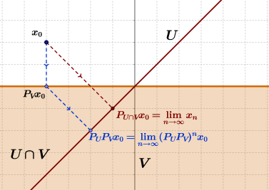
Figure 1: A GeoGebra [30] snapshot that illustrates Example 6.5. $U$ is the red line and $V$ is the shaded half-space. Shown also are the starting point $x_{0}$, the iterates of the MAP sequence $((P_{U}P_{V})^{n}x_{0})_{n\in{\mathbb{N}}}$ (which is eventually constant and equals to $\lim_{n\to\infty}(P_{U}P_{V})^{n}x_{0}$) and the limit $P_{U\cap V}x_{0}$ of the sequence $(x_{n})_{n\in{\mathbb{N}}}$ produced by Dykstra’s method.

Remark 6.6 (forward-backward vs. ADMM).

One can use the forward-backward method to solve 43 by setting $(f,g)=(\tfrac{1}{2}d^{2}_{U},\iota_{V})$. In this case the method reduces to MAP (see, e.g., [24, Example 10.12]) which is not DR (see, e.g., [4]). Therefore, in view of 3.2(i)&(ii) we conclude that the forward-backward method is not equivalent to ADMM.

Appendix A

Let $A\colon X\to X$ be linear. Define

$$q_{A}\colon X\to\mathbb{R}\colon x\mapsto\tfrac{1}{2}\langle x,Ax\rangle.$$ (50)

Recall that a linear operator $A\colon X\to X$ is monotone if $(\forall x\in X)$ $\langle x,Ax\rangle\geq 0$, and is strictly monotone if $(\forall x\in X\smallsetminus\{0\})$ $\langle x,Ax\rangle>0$. Let $h\colon X\to\mathbb{R}$ and let $x\in X$. We say that $h$ is Fréchet differentiable at $x$ if there exists a linear operator $Dh(x)\colon X\to\mathbb{R}$, called the Fréchet derivative of $h$ at $x$, such that $\lim_{0\neq\lVert y\rVert\to 0}\frac{h(x+y)-h(x)-Dh(x)y}{\lVert y\rVert}=0$; and $h$ is Fréchet differentiable on $X$ if it is Fréchet differentiable at every point in $X$. Also, we say that $h$ is Gâteaux differentiable at $x$ if there exists a linear operator $Dh(x)\colon X\to\mathbb{R}$, called the Gâteaux derivative of $h$ at $x$, such that $(\forall y\in X)$ $Dh(x)y=\lim_{\alpha\downarrow 0}\frac{h(x+\alpha y)-h(x)}{\alpha}$; and $h$ is Gâteaux differentiable on $X$ if it is Gâteaux differentiable at every point in $X$.

The following lemma is a special case of [7, Proposition 17.36].

Lemma A.1.

Let $A\colon X\to X$ be linear, strictly monotone, self-adjoint and invertible. Then the following hold:

1. $q_{A}$ and $q_{A^{-1}}$ are strictly convex, continuous, Fréchet differentiable and $(\nabla q_{A},\nabla q_{A^{-1}})=(A,A^{-1})$.

2. $q_{A}^{*}=q_{A^{-1}}$.

Proof. Note that, likewise $A$, $A^{-1}$ is linear, strictly monotone, self-adjoint (since $(A^{-1})^{*}=(A^{*})^{-1}=A^{-1}$) and invertible. Moreover, $\operatorname{ran}A=\operatorname{ran}A^{-1}=X$. (i): This follows from [7, Example 17.11 and Proposition 17.36(i)] applied to $A$ and $A^{-1}$ respectively. (ii): It follows from [7, Proposition 17.36(iii)], [StoerBulirsch02, Theorem 4.8.5.4] and the invertibility of $A$ that $q_{A}^{*}=q_{A^{-1}}+\iota_{\operatorname{ran}A}=q_{A^{-1}}+\iota_{X}=q_{A^{-1}}$. $\hfill\quad\blacksquare$

Proposition A.2.

Let $L\colon Y\to X$ be linear. Suppose that $L^{*}L$ is invertible. Then the following hold:

1. $\ker L=\{0\}$ .

2. $L^{*}L$ is strictly monotone.

3. $\operatorname{dom}(q_{L^{*}L}+g)^{*}=X$.

4. ${\partial}(q_{L^{*}L}+g)=\nabla q_{L^{*}L}+{\partial}g=L^{*}L+{\partial}g$.

5. $(q_{L^{*}L}+g^{*})^{*}$ is Fréchet differentiable on $X$.

6. $(L^{*}L+{\partial}g^{*})^{-1}$ is single-valued and $\operatorname{dom}(L^{*}L+{\partial}g^{*})^{-1}=X$.

7. $\operatorname{Prox}_{g^{*}\circ L^{*}}=\operatorname{Id}-L(L^{*}L+{\partial}g)^{-1}L^{*}$.

8. $\operatorname{Prox}_{(g^{*}\circ L^{*})^{*}}=L(L^{*}L+{\partial}g)^{-1}L^{*}$.

Proof. (i): Using [7, Fact 2.25(vi)] and the assumption that $L^{*}L$ is invertible we have $\ker L=\ker L^{*}L=\{0\}$. (ii): Using (i) we have $(\forall x\in X\smallsetminus\{0\})$ $\langle L^{*}Lx,x\rangle=\langle Lx,Lx\rangle=\lVert Lx\rVert^{2}>0$, hence $L^{*}L$ is strictly monotone. (iii): By (ii) and Lemma A.1(i) applied with $A$ replaced by $L^{*}L$ we have $\operatorname{dom}q_{L^{*}L}=\operatorname{dom}q^{*}_{L^{*}L}=X$, hence

$$\operatorname{dom}q_{L^{*}L}-\operatorname{dom}g=X-\operatorname{dom}g=X.$$ (51)

It follows from 51, [2, Corollary 2.1] and Lemma A.1(ii)&(i) that $\operatorname{dom}(q_{L^{*}L}+g)^{*}=\operatorname{dom}q_{L^{*}L}^{*}+\operatorname{dom}g^{*}=\operatorname{dom}q_{(L^{*}L)^{-1}}+\operatorname{dom}g^{*}=X+\operatorname{dom}g^{*}=X$. (iv): Combine 51, [2, Corollary 2.1] and Lemma A.1(i). (v): Since $q_{L^{*}L}$ is strictly convex, so is $q_{L^{*}L}+g$, which in view of [7, Proposition 18.9] and (iii) implies that $(q_{L^{*}L}+g)^{*}$ is Gâteaux differentiable on $X=\operatorname{int}\operatorname{dom}(q_{L^{*}L}+g)^{*}$. (vi): Using (iv), C.1(i) applied with $f$ replaced by $q_{L^{*}L}+g$, (v) and [7, Proposition 17.31(i)] we have $(L^{*}L+{\partial}g)^{-1}=({\partial}(q_{L^{*}L}+g))^{-1}={\partial}(q_{L^{*}L}+g)^{*}=\{\nabla(q_{L^{*}L}+g)^{*}\}$ is single-valued with $\operatorname{dom}(L^{*}L+{\partial}g)^{-1}=X$. (vii): Let $x\in X=\operatorname{dom}(L^{*}L+{\partial}g)^{-1}$ and let $y\in X$ such that $y=x-L(L^{*}L+{\partial}g)^{-1}L^{*}x$. Then using (vi) we have

$$x=y+Lu\quad\text{where}\quad u=(L^{*}L+{\partial}g)^{-1}L^{*}x.$$ (52)

Consequently, $L^{*}y+L^{*}Lu=L^{*}x\in L^{*}Lu+{\partial}g(u)$, hence $L^{*}y\in{\partial}g(u)$, equivalently, in view of C.1(i) applied with $f$ replaced by $g$, $u\in({\partial}g)^{-1}(L^{*}y)={\partial}g^{*}(L^{*}y)$. Combining with 52 we learn that

$$x\in y+L\circ({\partial}g^{*})\circ L^{*}(y).$$ (53)

Note that [7, Fact 2.25(vi) and Fact 2.26] implies that $\operatorname{ran}L^{*}=\operatorname{ran}L^{*}L=X$, hence $0\in\operatorname{sri}(\operatorname{dom}g^{*}-\operatorname{ran}L^{*})$. Therefore one can apply [7, Corollary 16.53(i)] to re-write 53 as $x\in(\operatorname{Id}+{\partial}(g^{*}\circ L^{*}))y$. Therefore, $y=\operatorname{Prox}_{g^{*}\circ L^{*}}x$ by [7, Proposition 16.44]. (viii): Apply C.1(ii) with $f$ replaced by $g^{*}\circ L^{*}$. $\hfill\quad\blacksquare$

Appendix B

In the following, we make use of the useful fact (see [39, Theorem 3.5.5])

$$f \Leftrightarrow f^{*}$$ is uniformly convex is uniformly smooth. (54)

Let $h\colon X\to\mathbb{R}$. We say that $h$ is uniformly smooth if there exists a function $\phi\colon\mathbb{R}_{+}\to\left[0,+\infty\right]$ (called the modulus of uniform smoothness) that vanishes at $0$ such that $(\forall(x,y)\in\operatorname{dom}f\times\operatorname{dom}f)$ $(\forall\alpha\in\left]0,1\right[)$ we have $f(\alpha x+(1-\alpha)y)+\alpha(1-\alpha)\phi(\lVert x-y\rVert)\geq\alpha f(x)+(1-\alpha)f(y)$.

Lemma B.1.

The following hold:

1. $g^{*}$ is uniformly smooth.

2. $g^{*}\circ L^{*}$ is uniformly smooth.

3. $(g^{*}\circ L^{*})^{*}$ is uniformly convex.

Proof. (i): Apply 54 with $f$ replaced by $g$. (ii): Suppose that $\phi$ is the modulus of uniform convexity of $g$. Using [1, Proposition 2.6(ii)] we learn that $g^{*}$ is uniformly smooth with modulus $\phi^{\#}\colon\left[0,+\infty\right[\to\left[0,+\infty\right]\colon s\mapsto\sup\big{\{}{rs-\phi(r)}~{}\big{|}~{}{r\geq 0}\big{\}}$. Moreover [1, Comment on page 708] implies that $\phi^{\#}$ is a nondecreasing function that vanishes only at $0$. Set $\psi\coloneqq\phi^{\#}(\lVert L^{*}\rVert\cdot)$ and note that [7, Fact 2.25(ii)] and A.2(i) imply that $\lVert L^{*}\rVert=\lVert L\rVert\neq 0$. Consequently, likewise $\phi^{\#}$, $\psi$ is a nondecreasing function that vanishes only at $0$. Let $(x,y)\in\operatorname{dom}f\times\operatorname{dom}f$ and let $\alpha\in\left]0,1\right[$. We claim that

$$(g^{*}\circ L^{*})(\alpha x+(1-\alpha)y)+\alpha(1-\alpha)\psi(\lVert x-y\rVert)\geq\alpha(g^{*}\circ L^{*})(x)+(1-\alpha)(g^{*}\circ L^{*})(y).$$ (55)

Indeed, we have $(g^{*}\circ L^{*})(\alpha x+(1-\alpha)y)+\alpha(1-\alpha)\psi(\lVert x-y\rVert)=g^{*}(\alpha L^{*}x+(1-\alpha)L^{*}y)+\alpha(1-\alpha)\phi(\lVert L^{*}\rVert\lVert x-y\rVert)\geq g^{*}(\alpha L^{*}x+(1-\alpha)L^{*}y)+\alpha(1-\alpha)\phi(\lVert L^{*}x-L^{*}y\rVert)\geq\alpha g^{*}(L^{*}x)+(1-\alpha)g^{*}(L^{*}y)=\alpha(g^{*}\circ L^{*})(x)+(1-\alpha)(g^{*}\circ L^{*})(y)$; equivalently $g^{*}\circ L^{*}$ is uniformly smooth with modulus $\psi$. (iii): Combine (ii) and 54 applied with $f$ replaced by $g^{*}\circ L^{*}$. $\hfill\quad\blacksquare$

Appendix C

We start by recalling the following well-known fact.

Fact C.1.

Let $f\colon X\to\left]-\infty,+\infty\right]$ be convex, lower semicontinuous and proper. Then the following hold:

1. $({\partial}f)^{-1}={\partial}f^{*}.$

2. $\operatorname{Prox}_{f}+\operatorname{Prox}_{f^{*}}=\operatorname{Id}$.

Proof. (i): See, e.g., [34, Remark on page 216] or [31, Théorème 3.1].

(ii): See, e.g., [7, Theorem 14.3(iii)]. $\hfill\quad\blacksquare$

Lemma C.2.

The Douglas–Rachford method given in 10 applied to the ordered pair $(f,g)$ with a starting point $x_{0}\in X$ to solve 9 can be rewritten as:

$$y_{n} =\operatorname{Prox}_{f}x_{n}$$ (56a)

$$x_{n+1} =y_{n}-\operatorname{Prox}_{g^{*}}(2y_{n}-x_{n}).$$ (56b)

Proof. Using 11, and C.1(ii) applied with $f$ replaced by $g$ we have

$$x_{n+1} =x_{n}-\operatorname{Prox}_{f}x_{n}+\operatorname{Prox}_{g}(2\operatorname{Prox}_{f}x_{n}-x_{n})=x_{n}-y_{n}+\operatorname{Prox}_{g}(2y_{n}-x_{n})$$

$$=x_{n}-y_{n}+2y_{n}-x_{n}-\operatorname{Prox}_{g^{*}}(2y_{n}-x_{n})=y_{n}-\operatorname{Prox}_{g^{*}}(2y_{n}-x_{n}),$$ (57)

and the conclusion follows. $\hfill\quad\blacksquare$

Appendix D

Proposition D.1.

Let $(x,y,z)\in X\times Y\times Z$. Then the following hold:

1. $B^{*}y=(A^{*}y,C^{*}y)$.

2. $\operatorname{dom}\widetilde{f}=\operatorname{dom}f\times\{0\}$.

3. $(\forall(x,z)\in\operatorname{dom}\widetilde{f})$ we have $z=0$ and $B(x,z)=Ax$.

4. $B(\operatorname{dom}\widetilde{f})=A(\operatorname{dom}f)$.

5. $0\in\operatorname{sri}(\operatorname{dom}g-B(\operatorname{dom}\widetilde{f}))$.

6. $\operatorname{argmin}(\widetilde{f}+g\circ B)=\operatorname{argmin}(f+g\circ A)\times\{0\}\neq\varnothing$.

7. $\operatorname{Prox}_{\widetilde{f}}(x,z)=(\operatorname{Prox}_{f}x,0)$.

8. $\operatorname{Prox}_{(g\circ B)^{*}}=B^{*}\operatorname{Prox}_{g^{*}}B$.

Proof. (i): Clear. (ii): It follows from 40 that $\operatorname{dom}\widetilde{f}=\operatorname{dom}f\times\operatorname{dom}\iota_{\{0\}}=\operatorname{dom}f\times\{0\}$. (iii): The claim that $z=0$ follows from (ii). Now combine with 38. (iv): Combine (ii) and (iii). (v): Combine (iv) and 34. (vi): It follows from (iii), (v) and 5 applied with $A$ replaced by $B$ that $\operatorname{argmin}(\widetilde{f}+g\circ B)=\operatorname{zer}({\partial}\widetilde{f}+B^{*}\circ{\partial}g\circ B)=\operatorname{zer}({\partial}f\times N_{\{0\}}+((A^{*}\circ{\partial}g\circ A)\times(C^{*}\circ{\partial}g\circ A)))=(\operatorname{zer}({\partial}f+A^{*}\circ{\partial}g\circ A)\times(\operatorname{zer}(N_{\{0\}}+C^{*}\circ{\partial}g\circ A)))$. Therefore, $(x,z)\in\operatorname{argmin}(\widetilde{f}+g\circ B)$ $\Leftrightarrow$ [$z=0$ and $x\in\operatorname{zer}({\partial}f+A^{*}\circ{\partial}g\circ A)$] $\Leftrightarrow$ $(x,z)\in\operatorname{argmin}(f+g\circ A)\times\{0\}$. No combine with 5. (v): Combine 40 and [7, Proposition 23.18]. (viii): Apply A.2(viii) with $(g,L)$ replaced by $(g^{*},B^{*})$ and use 38. $\hfill\quad\blacksquare$

References

• [1] D. Azé and J.-P. Penot, Uniformly convex and uniformly smooth convex functions, Annales de la faculté des Sciences de Toulouse $6^{e}$ série 4 (1995), 705–730.
• [2] H. Attouch and H. Brézis, Duality for the sum of convex functions in general Banach spaces, in Aspects of Mathematics and Its Applications 34 (1986), North-Holland, Amsterdam, 125–133.
• [3] H. Attouch and M. Théra, A general duality principle for the sum of two operators, Journal of Convex Analysis 3 (1996), 1–24.
• [4] H.H. Bauschke, J.Y. Bello Cruz, T.T.A. Nghia, H.M. Phan, and X. Wang, The rate of linear convergence of the Douglas–Rachford algorithm for subspaces is the cosine of the Friedrichs angle, Journal of Approximation Theory 185 (2014), 63–79.
• [5] H.H. Bauschke and P.L. Combettes, A Dykstra-like algorithm for two monotone operators, Pacific Journal of Optimization 4 (2008), 383–391.
• [6] H.H. Bauschke, R.I. Boţ, W.L. Hare and W.M. Moursi, Attouch–Théra duality revisited: paramonotonicity and operator splitting, Journal of Approximation Theory 164 (2012), 1065–1084.
• [7] H.H. Bauschke and P.L. Combettes, Convex Analysis and Monotone Operator Theory in Hilbert Spaces, Second Edition, Springer, 2017.
• [8] H.H. Bauschke and V.R. Koch, Projection methods: Swiss Army knives for solving feasibility and best approximation problems with halfspaces, Infinite Products and Their Applications, 1–40, Contemporary Mathematics, 636, Israel Mathematical Conference Proceedings.
• [9] A. Beck, First-Order Methods in Optimization, MOS-SIAM Series on Optimization, SIAM, 2017.
• [10] J.M. Borwein, Fifty years of maximal monotonicity, Optimization Letters 4 (2010), 473–490.
• [11] R.I. Boţ, E.R. Csetnek, ADMM for monotone operators: convergence analysis and rates (2017). arXiv:1705.01913v2[math.OC].
• [12] S. Boyd, N. Parikh, E. Chu, B. Peleato and J. Eckstein, Distributed optimization and statistical learning via the alternating direction method of multipliers, Foundations and Trends in Machine Learning 3 (2011), 1–122.
• [13] J.P. Boyle and R.L. Dykstra, A method for finding projections onto the intersection of convex sets in Hilbert spaces. Lecture Notes in Statistics 37 (1986), 28–47.
• [14] L.M. Brègman, The method of successive projection for finding a common point of convex sets, Soviet Mathematics Doklady  6 (1965), 688–692.
• [15] H. Brezis, Operateurs Maximaux Monotones et Semi-Groupes de Contractions dans les Espaces de Hilbert, North-Holland/Elsevier, 1973.
• [16] F. Riesz and B. Sz.-Nagy, Functional Analysis, Dover paperback, 1990.
• [17] R.S. Burachik and A.N. Iusem, Set-Valued Mappings and Enlargements of Monotone Operators, Springer-Verlag, 2008.
• [18] A. Chambolle and T. Pock, A first-order primal-dual algorithm for convex problems with applications to imaging, Journal of Mathematical Imaging and Vision 40 (2011), 120–145.
• [19] P.L. Combettes, The convex feasibility problem in image recovery, Advances in Imaging and Electron Physics 25 (1995), 155–270.
• [20] P.L. Combettes, Solving monotone inclusions via compositions of nonexpansive averaged operators, Optimization 53 (2004), 475–504.
• [21] L.M. Briceño-Arias and P.L. Combettes, A monotone + skew splitting model for composite monotone inclusions in duality, SIAM Journal on Optimization 21 (2011), 1230–1250.
• [22] P.L. Combettes and J.-C. Pesquet, Primal-dual splitting algorithm for solving inclusions with mixtures of composite, Lipschitzian, and parallel-sum type monotone operators, Set-Valued and Variational Analysis, published online, August 2011, http://dx.doi.org/10.1007/s11228-011-0191-y.
• [23] P.L. Combettes and J.-C. Pesquet, A proximal decomposition method for solving convex variational inverse problems, Inverse Problems 24, article 065014, (2008).
• [24] P.L. Combettes and J.-C. Pesquet, Proximal splitting methods in signal processing, in: Fixed-Point Algorithms for Inverse Problems in Science and Engineering, H.H. Bauschke et al. eds., Springer, New York, 185–212, (2011).
• [25] L. Condat, A primal-dual Splitting Method for Convex Optimization Involving Lipschitzian, Proximable and Linear Composite Terms, Journal of Optimization Theory and Applications 158, 460–479, (2013).
• [26] F. Deutsch, Best Approximation in Inner Product Spaces, Springer, 2001.
• [27] J. Eckstein, Splitting Methods for Monotone Operators with Applications to Parallel Optimization, Ph.D. thesis, MIT, 1989.
• [28] J. Eckstein and D.P. Bertsekas, On the Douglas–Rachford splitting method and the proximal point algorithm for maximal monotone operators, Mathematical Programming 55 (1992), 293–318.
• [29] D. Gabay, Applications of the method of multipliers to variational inequalities. In: M. Fortin, R. Glowinski (eds.) Augmented Lagrangian Methods: Applications to the Numerical Solution of Boundary-Value Problems, 299–331. North-Holland, Amsterdam (1983).
• [30] GeoGebra, http://www.geogebra.org.
• [31] J.-P. Gossez, Opérateurs monotones non linéaires dans les espaces de Banach non réflexifs, Journal of Mathematical Analysis and Applications, 34 (1971), 371–395.
• [32] P.L. Lions and B. Mercier, Splitting algorithms for the sum of two nonlinear operators, SIAM Journal on Numerical Analysis 16 (1979), 964–979.
• [33] D. O’Connor and L. Vandenberghe, On the equivalence of the primal-dual hybrid gradient method and Douglas–Rachford splitting. http://www.optimization-online.org/DB_HTML/2017/10/6246.html.
• [34] R.T. Rockafellar, On the maximal monotonicity of subdifferential mappings, Pacific Journal of Mathematics 33 (1970), 209–216.
• [35] R.T. Rockafellar and R. J-B Wets, Variational Analysis, Springer-Verlag, corrected 3rd printing, 2009.
• [36] S. Simons, Minimax and Monotonicity, Springer-Verlag, 1998.
• [37] S. Simons, From Hahn-Banach to Monotonicity, Springer-Verlag, 2008.
• [38] P. Tseng, Applications of a splitting algorithm to decomposition in convex programming and variational inequalities, SIAM Journal on Control and Optimization 29 (1991), 119–138.
• [39] C. Zălinescu, A new convexity property form monotone operators, Journal of Convex Analysis 13 (2006), 883–887.
• [40] E. Zeidler, Nonlinear Functional Analysis and Its Applications II/A: Linear Monotone Operators, Springer-Verlag, 1990.
• [41] E. Zeidler, Nonlinear Functional Analysis and Its Applications II/B: Nonlinear Monotone Operators, Springer-Verlag, 1990.