Quantum coherence in a compass chain under an alternating magnetic field

Abstract

We investigate quantum phase transitions and quantum coherence in a quantum compass chain under an alternating transverse magnetic field. The model can be analytically solved by the Jordan-Wigner transformation and this solution shows that it is equivalent to a two-component one-dimensional (1D) Fermi gas on a lattice. We explore mutual effects of the staggered magnetic interaction and multi-site interactions on the energy spectra and analyze the ground state phase diagram. We use quantum coherence measures to identify the quantum phase transitions. Our results show that $l_{1}$ norm of coherence fails to detect faithfully the quantum critical points separating a gapped phase from a gapless phase, which can be pinpointed exactly by relative entropy of coherence. Jensen-Shannon divergence is somewhat obscure at exception points. We also propose an experimental realization of such a 1D system using superconducting quantum circuits.

I Introduction

Many physical phenomena in quantum information science have evolved from being of purely theoretical interest to enjoying a variety of uses as resources in quantum information processing tasks. Throughout the development of the resource theory of entanglement, various measures were established. However, entanglement is not a unique measure of quantum correlation because separable states can have nonclassical correlations. The concept of quantum coherence has recently seen a surge of popularity since it serves as a resource in quantum information tasks Streltsov2017 , similar to other well-studied quantum resource such as the entanglement Osterloh2002 , quantum correlations Ollivier01 , and the randomness Bera17 . Baumgratz et al. Baumgratzq14 introduced a rigorous framework for the quantification of coherence based on resource theory and identified easily computable measures of coherence. Quantum coherence resulting from quantum state superposition plays a key role in quantum physics, quantum information processing, and quantum biology.

Ideally the coherence of a given state is measured as its distance to the closest incoherent state Girolami14 ; Bromley15 ; Streltsov15 ; Chitambar16 ; Killoran16 ; Winter16 ; Napoli16 ; Bagan16 ; Ma16 ; Streltsov16 ; Chitambar16a ; Chitambar16b ; Liu17a ; Bu17 ; Theurer17 ; Wang17 ; Zhang17 ; Hu17 . Coherence properties of a quantum state are usually attributed to the off-diagonal elements of its density matrix with respect to a selected reference basis. Among a few popular measures, there are three recently introduced coherence measures, namely, relative entropy of coherence, $l_{1}$ norm quantum coherence Baumgratzq14 , and Jensen-Shannon (JS) divergence Rad16 . The JS divergence and the $l_{1}$ norm of coherence obey the symmetry axiom of a distance measure while the relative entropy does not obey such distance properties. The $l_{1}$ norm of coherence sums up absolute values of all off-diagonal elements $\rho_{i,j}$ (with $i\neq j$) of the density matrix $\rho$, that is,

$$C_{l_{1}}(\rho) = \sum_{i\neq j}|\rho_{i,j}|,$$ (1)

where $\rho_{i,j}$ is the element of the density matrix with $i$ and $j$ being the row and the column index. $C_{l_{1}}(\rho)$ is a geometric measure that can be used as a formal distance measure. In parallel, the relative entropy has been established as a valid measure of coherence for a given basis:

$$C_{\rm re}({\rho}) = S({\rho}||{\rho}_{\rm diag})=S({\rho}_{\rm diag})-S({\rho}),$$ (2)

where $S(\rho)=-{\rm Tr}(\rho\log_{2}\rho)$ stands for the von Neumann entropy and ${\rho}_{diag}$ is the incoherent state obtained from ${\rho}$ by removing all its off-diagonal entries. $C_{l_{1}}$ and $C_{\rm re}$ are known to obey strong monotonicity for all states. Since $C_{\rm re}$ is similar with relative entropy of entanglement, it has a clear operational interruption as the distillable coherence. Meanwhile, $C_{l_{1}}$ takes an operational interpretation as the maximum distillable coherence from a resource theoretical viewpoint Rana17 ; Zhu17 . It was shown that $C_{l_{1}}$ is an upper bound for $C_{\rm re}$ for all pure states and qubit states Rana16 . Moreover, the measure of quantum coherence based on the square root of the JS divergence is given by

$$C_{\rm JS}({\rho})=\sqrt{S\left(\frac{\rho_{\rm diag}+{\rho}}{2}\right)-\frac{1}{2}S({\rho}_{\rm diag})-\frac{1}{2}S({\rho})}.$$ (3)

The JS divergence is known to be a symmetric and bounded distance measure between mixed quantum states Majtey05 and is exploited to study shareability of coherence Rad16 . We remark that these coherence measures are all basis dependent Malvezzi16 .

Currently, approaches adopted from quantum information theory are being tested to explore many-body theory from another perspective and vice versa. Various quantum resource measures have been exploited to characterize the state of many-body systems and the associated quantum phase transitions (QPTs). A QPT occurs at zero temperature and is engraved by a qualitative change solely due to quantum fluctuations as a non-thermal parameter is varied. Quantum entanglement and quantum discord have been proven to be fruitful to investigate QPTs. For instance, entanglement entropy changes at some (but not all) QPTs You15 . Investigation of entanglement spectra is therefore very useful and helps to identify a possible QPT when the entanglement entropy in the ground-state changes by a finite value when Hamiltonian parameters are varied. One of easily accessible parameters is a magnetic field which might control producing quantum matter near a quantum critical point (QCP) in spin chains Bla18 . Small systems of interacting spins in a two-dimensional (2D) compass model with perturbing interactions could also be used for quantum computation Tro12 .

Quantum coherence has emerged from an information physics perspective to address different aspects of quantum correlation in a many-body system. Comparing with entanglement measures, quantum coherence is expected to be capable of detecting QPTs even when the entanglement measures fail to do so. One can easily recognize that entanglement may be a form of coherence and the converse is not necessarily valid. For instance, a product state ($|0\rangle+|1\rangle)\otimes(|0\rangle+|1\rangle$), for a two-qubit system carries coherence but not entanglement. That is to say, quantum coherence incarnates a different feature of a quantum state from entanglement. On the other hand, coherence measures can be used as a resource in quantum computing protocols, and one may claim that they are more fundamental. So a comparative study of these measures for characterizing QPTs in various spin chain models is a potential research topic, which may be valuable in both physical theory and experiment.

To test the validity of this approach, the Ising model is the most transparent example of the importance of exactly soluble models as guides along this difficult path. All coherence measures are able to locate the Ising-type second-order transition. Here we consider another prominent model dubbed as a one-dimensional (1D) compass model for a $p$-wave superconducting chain, which sustains more complex physical phenomena than the Ising model, such as macroscopic degeneracy Brzezicki07 , pure classical features You12 , and suppressed critical revival structure Jafari17 .

The purpose of this paper is to investigate QPTs and quantum coherence in the 1D quantum compass model (QCM) under an alternating transverse magnetic field. The motivation is twofold. On the one hand, previous investigations revealed that the 1D compass model could exhibit miscellaneous phases via modulation of external fields. An exotic spin-liquid phase can emerge through a Berezinskii-Kosterlitz-Thouless (BKT) QPT under a uniform magnetic field. We would like to verify whether such a transition is robust under realistic inhomogeneity of external fields You14 . The calculations take into account both uniform and staggered fields. On the other hand, its exact solvability provides a suitable testing ground for calculating accurately coherence measures to detect QPTs. We investigate the coherence of this model in the thermodynamic limit and its connection to QPTs.

The remaining of the paper is structured as follows. An overview of the 1D compass model with staggered magnetic fields is presented in Sec. II. We consider the cases in the presence of a uniform and an alternating transverse magnetic field, and discuss a possible experimental realization using superconducting quantum circuits in Sec. III. The model is extended by adding three-site interactions in Sec. IV. Next the model is exactly solved and QPTs are studied. We present the calculations of quantum coherence measures in Sec. V. A final discussion and summary are presented in Sec. VI.

II The Model and Its Analytical Solution

We begin with a generic 1D QCM Brzezicki07 on a ring of $N$ sites, where $N$ is even. The Hamiltonian describes a competition between two pseudospin $\tau=1/2$ components, $\{\sigma^{x}_{i},\sigma^{y}_{i}\}$, which reads,

$$\cal{H}_{\rm QCM} = \sum_{i=1}^{N/2}\left(J_{1}\,X_{2i-1,2i}+J_{2}\,Y_{2i,2i+1}\right),$$ (4)

and has the highest possible frustration of interactions. Here $X_{i,j}\equiv\sigma_{i}^{x}\sigma_{j}^{x}$, $Y_{i,j}\equiv\sigma_{i}^{y}\sigma_{j}^{y}$, and $\sigma_{i}^{\alpha}$ is a Pauli matrix. $J_{1}$ ($J_{2}$) stands for the amplitude of the nearest neighbor interaction on odd (even) bonds. This model owns a particular intermediate symmetry, which allows for $N/2$ mutually commuting $\mathbb{Z}_{2}$ invariants $Y_{2i-1,2i}$ ($X_{2i,2i+1}$) in the absence of the transverse field term, and presents distinct features. The ground state possesses a macroscopic degeneracy of at least $2^{(N/2-1)}$ in the structure of the spin Hilbert space Brzezicki07 ; You14 . The intermediate symmetries also admit a dissipationless energy current Qiu16 . The 1D QCM Eq. (4) can be transformed to the fermion language and next diagonalized, see the Appendix. In fact, the model can be described by a two-component 1D Fermi gas on a lattice as displayed in Eq. (32).

The 1D QCM in Eq. (4) may be supplemented by a possibly spatially inhomogeneous Zeeman field $\vec{h}_{i}$, given by

$$\cal{H}_{\rm h} = \sum_{i=1}^{N}\vec{h}_{i}\cdot\vec{\sigma}_{i}.$$ (5)

In a realistic structure, the crystal fields surrounding the odd-indexed sites and even-indexed sites are different. The presence of two crystallographically inequivalent sites on each chain with a low symmetry of the crystal structure leads to staggered gyromagnetic tensors.

It has been recently shown that a spatially varying magnetic field can be induced by an effective spin-orbit interaction. The alternating spin environment is represented by the staggered Dzyaloshinskii-Moriya interaction and Zeeman terms. The staggered magnetic field plays an important role in understanding the field dependence of the gap in Cu benzoate antiferromagnetic chain Affleck99 ; Fledderjohann96 ; Zhao03 ; Kenzelmann04 and in Yb₄As₃ Kohgi01 . We remark that there is increasing interest in the effects of the staggered field motivated by the experimental work on a number of materials. The interplay between the staggered Zeeman fields and dimerized hopping on the topological properties of Su-Schrieffer-Heeger (SSH) model has received much attention only recently SSH , after the rapid progress in the synthesis of 1D heterostructures Sau10 ; Alicea10 ; Das12 ; Perge14 .

Without the loss of generality, we consider a staggered magnetic field, i.e., $\vec{h}_{2i-1}$=$h_{1}\hat{z}$, $\vec{h}_{2i}$=$h_{2}\hat{z}$, $\forall i=1,\cdots,N/2$. Be aware that $h_{i}=g_{i}\mu_{B}B_{i}$ here is the reduced magnetic field containing the $g$-factor and the Bohr magneton $\mu_{\rm B}$. An effective staggered magnetic field might be attributed to the alternating $g$ tensor in an applied uniform field Feyerherm2000 . Thereby, we define an average magnetic field $h=(h_{1}+h_{2})/2$ and a field difference $\delta=(h_{2}-h_{1})/2$. The 1D compass model in external field,

$$\cal{H} = \cal{H}_{\rm QCM}+\cal{H}_{\rm h},$$ (6)

is exactly soluble and we obtain its zero-temperature phase diagram, see below. For the sake of clarity, we briefly describe the procedure to diagonalize the Hamiltonian Eq. (6) exactly in the Appendix.

Thus the Hamiltonian (6) in the Bogoliubov-de Gennes (BdG) form in terms of Nambu spinors is:

$$\cal{H} = \frac{1}{2}\sum_{k}\Upsilon_{k}^{\dagger}\hat{H}_{k}\Upsilon_{k},$$ (7)

where $\Upsilon_{k}^{\dagger}=(a_{k}^{\dagger},b_{k}^{\dagger},a_{-k},b_{-k})$. In this circumstance, the Hamiltonian (6) reads

$$\hat{H}_{k} = 2\delta\Gamma_{zz}-2h\Gamma_{z0}+T^{r}_{k}(\Gamma_{zx}-\Gamma_{yy})-T^{i}_{k}(\Gamma_{zy}+\Gamma_{yx}),$$

with $\Gamma_{ab}=\tau^{a}\otimes\sigma^{b}$, $\forall$ $a,b=x,y,z$, and $\tau^{x,y,z}$/$\sigma^{x,y,z}$ being the Pauli matrices acting on particle-hole space and spin space, respectively, and $\tau^{0}=\sigma^{0}$ is a 2$\times$2 unit matrix. Here $T_{k}^{r}$ and $T_{k}^{i}$ are the real and imaginary parts of $T_{k}=J_{1}+J_{2}e^{ik}$. The BdG Hamiltonian Eq. (LABEL:HamiltonianMatrix2) respects a particle-hole symmetry defined as ${\cal C}\hat{H}(k){\cal C}^{-1}=-\hat{H}(-k)$ with ${\cal C}=\Gamma_{x0}\cal{K}$, where $\cal{K}$ is the complex conjugate operator. As a consequence the energy levels appear in conjugate pairs such as $\varepsilon(k)$ and $-\varepsilon(-k)$. The diagonal form of the Hamiltonian Eq. (LABEL:HamiltonianMatrix2) is then given by,

$${\cal H}=\sum_{k}\sum_{j=1}^{2}\varepsilon_{k,j}\left(\gamma_{k,j}^{\dagger}\gamma_{k,j}-\frac{1}{2}\right).$$ (9)

The spectra consist of two branches of energies $\varepsilon_{k,j}$ (with $j=1,2$), given by the following expressions:

$$\varepsilon_{k,1(2)}=\sqrt{|T_{k}|^{2}+4h^{2}}\pm\sqrt{|T_{k}|^{2}+4\delta^{2}}.$$ (10)

The ground-state energy per site for $h>\delta$ may be expressed as

$$e_{0}=-\frac{2}{N}\sum_{k}\sqrt{J_{1}^{2}+J_{2}^{2}+2J_{1}J_{2}\cos k+4h^{2}}.$$ (11)

The advantage of the result given by Eq. (11) is that $e_{0}$ is independent of $\delta$ as well as of the signs of $J_{1}$ and $J_{2}$. The intersite correlators are given by the Hellmann-Feynman theorem:

$$\langle\sigma^{x}_{2i-1}\sigma^{x}_{2i}\rangle=-\frac{2}{N}\sum_{k}\frac{J_{1}+J_{2}\cos k}{\sqrt{J_{1}^{2}+J_{2}^{2}+2J_{1}J_{2}\cos k+4h^{2}}},$$

$$\langle\sigma^{y}_{2i}\sigma^{y}_{2i+1}\rangle=-\frac{2}{N}\sum_{k}\frac{J_{2}+J_{1}\cos k}{\sqrt{J_{1}^{2}+J_{2}^{2}+2J_{1}J_{2}\cos k+4h^{2}}}.$$

(12)

For $\delta>h$, an interchange between $h$ and $\delta$ is performed in Eqs. (11-12).

Since a QPT occurs only when the gap closes, looking for gapless points in the energy spectrum may indicate this transition. The lower mode $\varepsilon_{k,2}$ reduces to a zero-energy flat band for $h=\pm\delta$, corresponding to either $h_{2i-1}=0$ or $h_{2i}=0$. This undermines the limited condition for the existence of a macroscopic degeneracy in the ground-state manifolds. The zero-energy flat band is fragile against an infinitesimal external uniform magnetic field for $\delta=0$. A uniform field will remove the ground-state degeneracy and the bands are no longer degenerate. The result here implies that a magnetic field applied on one sublattice still makes the zero-energy flat band intact.

Interestingly, the model possesses local symmetries that one can find in the absence of field terms at odd sites. If field $h_{2i-1}$ is vanishing at odd sites and at even sites it takes any random values, then any eigenstate has $2^{(N/2-1)}$ degeneracy for a ring of length $N$. These degeneracies follow from the symmetry operators,

$$S_{2i}\equiv\sigma^{y}_{2i-1}\otimes\sigma^{z}_{2i}\otimes\sigma^{x}_{2i+1},$$ (13)

and are activated when the field is absent at odd sites. Such symmetry operators (13) anti-commute for the neighbors, i.e., $\{S_{2i},S_{2(i+1)}\}=0$, while they commute otherwise.

III Possible experimental realization using superconducting quantum circuits

The unique features of this rich model (6) motivate us to consider its possible physical implementations to advance our understandings. It is well known that superconducting circuit systems have become one of the leading platforms for scalable quantum computation, quantum simulation and demonstrating quantum optical phenomena because of its exotic properties such as controllability, flexibility, scalability, and compatibility with micro-fabrication Wen05 ; you2005pt ; Dev13 . Various models of many-body systems have been proved to be able to be simulated by superconducting circuits, such as the Kitaev lattice You10 , the Heisenberg spin model Her14 , the fermionic model Bar15 , the 1D Ising model Bar16 and anisotropic quantum Rabi model Wang18 . In our case, the 1D compass chain in Eq. (6) can be built from superconducting charge qubits, each of which is composed of a direct current superconducting quantum interference device (dc SQUID) with two identical Josephson junctions. For $i$th charge qubit, the gate voltage $V_{gi}$ applied through the gate capacitance $C_{gi}$ can be used to control the charge, and the magnetic flux $\Phi_{ei}$ piercing the SQUID can be used to control the effective Josephson energy, $E_{J}(\Phi_{ei})=2E_{J}\cos(\pi\Phi_{ei}/\Phi_{0})$.

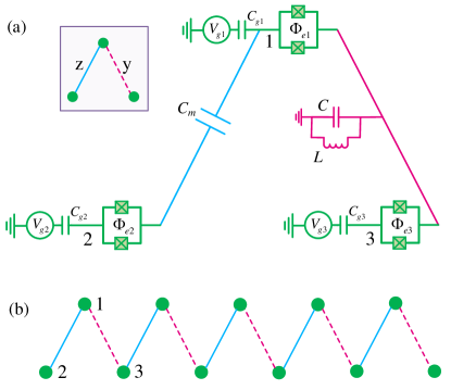
Figure 1: Scheme of a circuit QED system for the physical implementation of the 1D compass chain Hamiltonian Eq. (6): (a) Design of the basic building block, which is composed of three superconducting charge qubits, labeled as $1,~{}2,~{}3$. Qubits 1 and 2 are coupled capacitively to each other via a mutual capacitance $C_{m}$; and the coupling between the qubits 1 and 3 are provided by a commonly-shared LC oscillator. Inset: the orange circles denote the superconducting charge qubits; the two types of inter-qubit couplings are denoted as $z$- and $y$-bond, which are indicated by the blue-solid and the red-dashed line, respectively. (b) A 1D compass chain constructed by repeating the building block in (a).

It has been demonstrated that charge qubits can be coupled to each other for all the individual interactions of Ising type Wen05 , i.e., $\propto\sigma_{i}^{x}\sigma_{i+1}^{x}$ via a mutual inductance you2002prl , $\propto\sigma_{i}^{y}\sigma_{i+1}^{y}$ via an LC oscillator Mak99 , and $\propto\sigma_{i}^{z}\sigma_{i+1}^{z}$ via a capacitor pashkin2003n . This provides us a promising way to implement the 1D compass chain with the superconducting charge qubits. As shown in Fig. 1, a charge qubit is placed at each node, and is then connected to its two nearest neighbors with two types of couplers, i.e., a capacitor for the $z$-type bond and an LC oscillator for the $y$-type bond.

For the sake of simplicity and without the loss of generality, we assume all the charge qubits to be identical such that $C_{gi}\equiv C_{g}$, $E_{Ji}\equiv E_{J}$, $E_{Ci}\equiv E_{C}$. Following the standard quantization procedure of the circuit by firstly writing down the kinetic energy and the potential energy of the circuit, and secondly choosing the average phase drop $\varphi_{i}$ of each charge qubit as the canonical coordinate, the Hamiltonian of the entire system can then be obtained by a Legendre transformation.

We consider the situation when the frequency of the LC oscillator is much larger than the frequency of the qubit. In this case the LC oscillator is not really excited and the corresponding terms can be removed from the total Hamiltonian. Even though, the LC oscillator’s virtual excitation still produces an effective coupling between the corresponding charge qubits. For charge qubit with $E_{C}\gg E_{J}$, at very low temperature, the two-level system is formed by the charge states $|0\rangle$ and $|1\rangle$, which denote the zero and one extra Cooper pair on the island, respectively. After projecting the total Hamiltonian into the $i$th charge qubit’s computational basis $\{|0\rangle_{i},|1\rangle_{i}\}$, we obtain You10 ,

$$H=J_{i,j}^{y}\!\sum_{y-{\rm links}}\sigma_{i}^{y}\sigma_{j}^{y}+J_{i,j}^{z}\!\sum_{z-{\rm links}}\sigma_{i}^{z}\sigma_{j}^{z}+\sum_{i}h_{i}^{x}\sigma_{i}^{x},$$ (14)

where all the charge qubits are biased at the optimal point (i.e., $n_{gi}=C_{g}V_{gi}/{(2e)=1/2}$) such that $h_{i}^{z}=0$, and $h_{i}^{x}=-E_{J}\cos(\pi\Phi_{ei}/\Phi_{0})$ is the effective Josephson energy of the $i$th charge qubit, $\Phi_{0}\equiv h/2e$ is the flux quantum. The $y$-type Ising coupling strength

$$J_{i,j}^{y}=-4\xi E_{J}^{2}\cos\left(\pi\Phi_{ei}/\Phi_{0}\right)\cos\left(\pi\Phi_{ej}/\Phi_{0}\right)\leq 0,$$ (15)

with $\xi=L\pi^{2}{(2C_{J}+C_{g}+C_{m})}^{2}{(C_{g}+C_{m})}^{2}/{(\Lambda\Phi_{0})}^{2}$, are tunable via the external magnetic flux threading the SQUIDs in the $i$th and $j$th charge qubits. Simultaneously the $z$-type coupling strength is fixed as

$$J_{i,j}^{z}=\frac{e^{2}C_{m}}{\Lambda}\geq 0,$$ (16)

with $\Lambda=(2C_{J}+C_{g}+C_{m})^{2}-C_{m}^{2}$. A detailed analysis of circuit quantization can be found in Ref. You10 .

An intuitive understanding of the coupling mechanism in the Hamiltonian Eq. (14) would be the following. Each charge qubit is coupled to its left or right nearest neighbor via a capacitor or an LC oscillator. The appearance of a capacitor modifies the electrostatic energy of the system, and thus provides the $z$-type Ising coupling. On the other hand, the magnetic energy of the inductor is biased by a current composed of contributions from both of the two qubits, and thus the virtually excited LC oscillator induces the $y$-type Ising coupling. Then implementing a unitary rotation around the $y$ axis, i.e., $U\equiv\prod_{j}e^{i\pi\sigma_{j}^{z}/4}$, one can find $U\sigma_{i}^{x}U^{\dagger}=\sigma_{i}^{z}$, $U\sigma_{i}^{z}U^{\dagger}=-\sigma_{i}^{x}$, and then Eq. (14) can be recast into the Hamiltonian Eq. (6).

IV Effect of three-site interactions

To make the model as general as possible and still exactly soluble, we introduce in addition three-site interactions of the (XZX$+$YZY)-type into Eq. (6) ,

$$\cal{H}_{\rm 3-site} = J_{3}\sum_{i=1}^{N}\left(X_{i-1,i+1}+Y_{i-1,i+1}\right)Z_{i},$$ (17)

where $J_{3}$ characterizes their strength. Such interactions between three adjacent sites emerge as an energy current of a compass chain in the nonequilibrium steady states Qiu16 . Three-site interactions violate the intermediate symmetry and elicit exotic phenomena. This generalized version of the 1D QCM has been shown to host a diversity of nontrivial topological phases and an emergent BKT QPT under the interplay of a perpendicular Zeeman field and multi-site interactions You17 .

We next turn to the discussion of the physical implementation of the 1D QCM including the three-site interaction with superconducting circuits. As superconducting circuits offer advantages of easy tunability and scalability, in principle, many-body interactions in superconducting systems could be designed using Josephson-junction-based couplers in a graph structure bergeal2010np ; chancellor2017nqi ; leib2016qst . However, the effective many-body coupling terms may emerge with a much weaker strength. An alternative and practical strategy to generate many-body interactions would be the simulation protocols employing the microwave fields with appropriate frequency conditions, as have been studied in nuclear magnetic resonance systems zhang2006pra , optical lattices buchler2007np , and superconducting circuits sameti2017pra ; marvian2017pra . Therefore, we expect that the three-site interactions of the sort of XZX$+$YZY-type as in Eq. (17) would be built in similar fashions. However, an in-depth study of experimental implementation of this particular model will be left for future investigation.

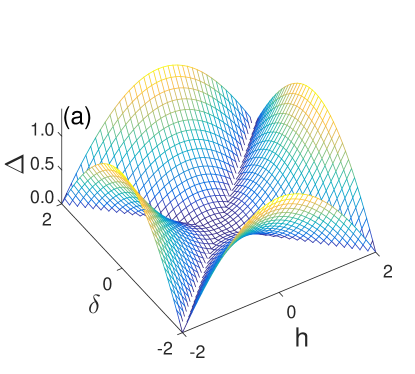
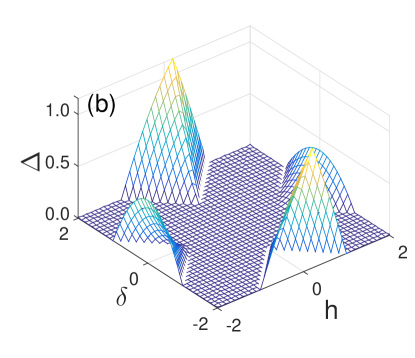
Figure 2: Three-dimensional plot of the energy gap as a function of $h$ and $\delta$ for: (a) $J_{3}=0$ and (b) $J_{3}=1$. Parameters are as follows: $J_{1}=1$, $J_{2}=4$.

Figure 3: The electron spectra $\varepsilon_{k,2}$ and its corresponding hole spectra $-\varepsilon_{k,2}$ for increasing magnetic field $h$ in Eq. (18): (a) $h=-3$, (b) $h=-2.5$, (c) $h=-2.0$, (d) $h=-1.5$, (e) $h=0$, (f) $h=1.5$, (g) $h=2$, (h) $h=2.5$, and (i) $h=3$. Parameters are as follows: $J_{1}=1$, $J_{2}=4$, $J_{3}=2$, and $\delta=0.5$.

The generalized Hamiltonian of the 1D QCM which includes the three-site (XZX$+$YZY) interaction is

$${\cal H}=\cal{H}_{\rm QCM}+\cal{H}_{\rm h}+\cal{H}_{\rm 3-site}.$$ (18)

Eq. (18) describes a 1D $sp$-chain with inter-band interactions and hybridization between orbitals Puel15 . The three-site interactions can be converted into fermionic form ${\cal H}_{\rm 3-site}=4J_{3}\sum_{k}\cos k\,c_{k}^{\dagger}c_{k}$. We note that the spectra can be pinpointed at commensurate momenta $k=\pm\pi/2$ regardless of the value of $J_{3}$. Hence the eigenspectra (10) can be renormalized with $-2h\to F_{k}=-2h+2J_{3}\cos k$, as evidenced in Eq. (52).

The main features and the evolution of these profiles under staggered fields with increasing magnetic field $h$ are depicted in Fig. 3. We observe that the ground state of the system is complicated under the interplay of three-site interactions and staggered magnetic field. As $h$ rises from large negative values, $\varepsilon_{k,2}$ closes the gap gradually and finally touches $\varepsilon=0$ at momentum $k=\pi$ for $h=-|J_{3}+\delta|$. Further increase of $h$ bends $\varepsilon_{k,2}$ downwards, leading to $\varepsilon_{|k|>|k_{ic}|,2}<0$ with an incommensurate momentum $k_{ic}$. An additional crossing at $k=\pi$ revives for $h=-|J_{3}-\delta|$. We can see that the number of crossing points at zero energy grows from 0 to 4 in Figs. 3(a)-3(e), and then decreases with further increase of $h$, see Figs. 3(f)-3(i). Altogether, the number of Fermi points at which the linear dispersion relation is found changes as $h$ increases. Indeed, here the topological transition belongs to the universality of the Lifshitz transition.

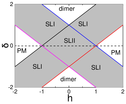
Figure 4: Phase diagram of the compass chain (18) in an alternating transverse field. The shaded regions mark the gapless spin-liquid phase, in which SLI (SLII) denotes the spin-liquid phase I (II) with 2 (4) Fermi nodes. The dashed line marks the path $\delta=0$. Other parameters: $J_{1}=1$, $J_{2}=4$, $J_{3}=1$.

It is also easy to see that the Weyl points collapse at $h=\pm|J_{3}+\delta|$ with increasing $h$. In the gapless phase the crossings between bands exhibit a linear dispersion relation [see Figs. 3(c)-3(g)] and thus define effective 1D Weyl modes. One notes that the nodes appear and disappear only when two nodes are combined, as a characteristic of Weyl fermions in a three-dimensional or 2D superconductor Yang14 ; Neu16 and in topological superfluidity Cao14 ; Pav15 ; Brz17 ; Brz18 . It is noticed with the emergence of two Weyl points at its extremities ($k=\pm\pi$) and their collapse at the center of the Brillouin zone ($k=0$). In this region the low-energy Hamiltonian with Weyl nodes in a 1D system can be reduced to describe the two Bogoliubov bands that cross zero energy.

The resulting phase diagram of the model Eq. (18), obtained by the exact solution using the Jordan-Wigner transformation, is shown in Fig. 4. For clarity we have considered the entire plane of fields, although the phase diagram is obviously symmetric under reflection from the $h_{1}=h_{2}$ and $h_{1}=-h_{2}$ lines, which also symmetrize the spectrum and entanglement. The quantum phase boundaries are determined by the following condition:

$$|h|+|\delta|=J_{3}.$$ (19)

For large $h$, the system changes to a disordered paramagnetic (PM) phase, in which the $z$-axis sublattice magnetizations are unbiased, as shown in Fig. 5(a). On the contrary, the dimer phase is the one in which $z$-axis magnetization at odd and even sites has a staggered order.

The staggered magnetic susceptibilities are vanishing in the both gapped phases, while they are finite in the gapless phases. Besides, as shown in Fig. 5(b), the nearest neighbor correlation $\langle\sigma_{2i-1}^{y}\sigma_{2i}^{y}\rangle$ clearly shows nonanalytical behavior at the QCPs, and the counterpart $\langle\sigma_{2i-1}^{x}\sigma_{2i}^{x}\rangle$ is smooth. One can notice that a singular behavior can be detected by taking the first derivative of $\langle\sigma_{2i-1}^{x}\sigma_{2i}^{x}\rangle$ and $\langle\sigma_{2i}^{y}\sigma_{2i+1}^{y}\rangle$ with respect to $h$.

Since QPTs are caused by nonanalytical behavior of ground-state energy, QCPs correspond to zeros of $\varepsilon_{k,2}$. The gap vanishes as $\Delta\sim(h-h_{c})^{\nu z}$, where $\nu$ and $z$ are the correlation-length and dynamic exponents, respectively. The gap is determined by the condition, $\partial\varepsilon_{k=k_{0},2}/\partial k=0$ and one finds $\Delta=\min_{k}|\varepsilon_{k,2}|$. This implies that the minimum is suited at either $k_{0}=0$ or $k_{0}=\pi$, depending which mode has a lower energy. One finds the critical exponents satisfy $\nu z=1$, as revealed in Fig. 2(b). The expansion of the energy spectra at the criticality around the critical mode $k_{0}$, i.e., at $\Delta k\equiv k-k_{0}\ll 1$, $\partial\varepsilon_{k,2}\sim 2J_{3}\delta(\Delta k)^{2}/\sqrt{(J_{1}+J_{2}\cos k_{0})^{2}+4\delta^{2}}$. The quadratic dispersion in Fig. 3(b) suggests a dynamical exponent $z=2$ and hence $\nu=1/2$, which is different from the generic QCM in the absence of three-site interactions Sun09a ; Motamedifar13 .

Remarkably, the ground state develops weak singularities at $\delta=0$. For $\delta=0$ the phase boundaries are pinpointed at $h_{c}=\pm J_{3}$ with an incommensurate critical momentum $k_{0}=\cos^{-1}(h/J_{3})$, as presented in Fig. 2(b). One can find that the system transforms from the gapped phase to the gapless phase passing through an unconventional field-induced QCP, where infinite-order QPTs occur by tuning $h$ along the path (Fig. 4, dashed line) to approach the QCPs, with no broken-symmetry order parameter. We can identify that $h_{c}=\pm J_{3}$ are multi-critical points, where $h-\delta=\pm J_{3}$ and $h+\delta=\pm J_{3}$ meet You17 . One finds the critical exponents that follow $\nu z=2$ by observing the gap scaling. The dependence of low-energy excitations on $k$ shows that $z=2$ in the gapless phase while $z=4$ at QCPs. It has been shown that $z$ can be extracted from the measurement of the low-temperature specific heat and entropy in the Tomonaga-Luttinger liquid phase Kono15 .

V Quantum coherence measures

In the representation spanned by the two-qubit product states we employ the following basis,

$$\{|0\rangle_{i}\otimes|0\rangle_{j},|0\rangle_{i}\otimes|1\rangle_{j},|1\rangle_{i}\otimes|0\rangle_{j},|1\rangle_{i}\otimes|1\rangle_{j}\},$$ (20)

where $|0\rangle$ ($|1\rangle$) denotes spin up (down) state, and the two-site density matrix can be expressed as,

$$\rho_{ij}=\frac{1}{4}\sum_{a,a^{\prime}=0}^{3}\left\langle\sigma_{i}^{a}\sigma_{j}^{a^{\prime}}\right\rangle\,\sigma_{i}^{a}\sigma_{j}^{a^{\prime}},$$ (21)

where $\sigma_{i}^{a}$ stands for Pauli matrices $\{\sigma_{i}^{x},\sigma_{i}^{y},\sigma_{i}^{z}\}$ with $a=1,2,3$, and for a $2\times 2$ unit matrix with $a=0$. Since the Hamiltonian has $\mathbb{Z}_{2}$ global phase-flip symmetry, the two-qubit density matrix reduces to an $X$ state,

$$\rho_{ij}=\left(\begin{array}[]{cccc}u_{+}&0&0&z_{-}\\ 0&w_{+}&z_{+}&0\\ 0&z_{+}^{*}&w_{-}&0\\ z_{-}^{*}&0&0&u_{-}\end{array}\right),$$ (22)

with

$$u_{\pm} = \frac{1}{4}\left(1\pm\langle{\sigma_{i}^{z}}\rangle\pm\langle{\sigma_{j}^{z}}\rangle+\langle{\sigma_{i}^{z}\sigma_{j}^{z}}\rangle\right),$$ (23)

$$z_{\pm} = \frac{1}{4}\left(\langle\sigma_{i}^{x}\sigma_{j}^{x}\rangle\pm\langle\sigma_{i}^{y}\sigma_{j}^{y}\rangle\right),$$ (24)

$$\omega_{\pm} = \frac{1}{4}\left(1\pm\langle{\sigma_{i}^{z}}\rangle\mp\langle{\sigma_{j}^{z}}\rangle-\langle\sigma_{i}^{z}\sigma_{j}^{z}\rangle\right).$$ (25)

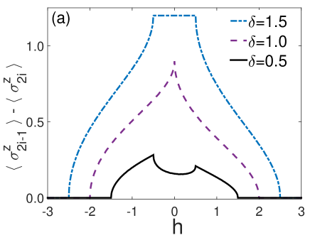
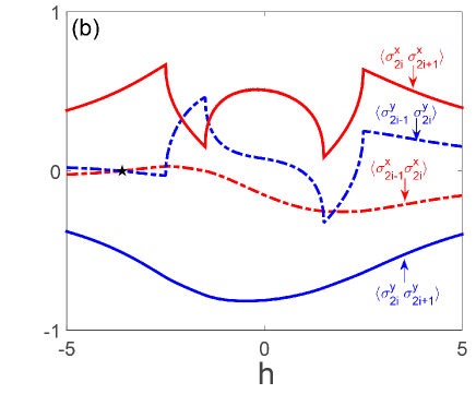
Figure 5: Effect of alternating magnetic field in the 1D compass model (18): (a) the difference between odd-site and even-site magnetization for $\delta=0.5$, 1.0 and 1.5 with $J_{3}=1$; (b) the nearest-neighbor correlations $\langle\sigma_{i}^{\alpha}\sigma_{i+1}^{\alpha}\rangle$ ($\alpha=x$, $y$) on odd bonds and even bonds with $J_{3}=2$, $\delta=0.5$. The symbol $\star$ in (b) marks the position of $\langle\sigma_{2i-1}^{x}\sigma_{2i}^{x}\rangle=\langle\sigma_{2i-1}^{y}\sigma_{2i}^{y}\rangle=0$. Other parameters are: $J_{1}=1$, $J_{2}=4$.

Note that the formula can be simplified when the system is translation invariant, i.e., $\langle\sigma_{i}^{z}\rangle=\langle\sigma_{j}^{z}\rangle$ for arbitrary $i$ and $j$, such that $\omega_{+}=\omega_{-}$. Under the staggered magnetic field, the magnetization densities $\{\langle\sigma_{2i-1}^{z}\rangle\}$ at odd sites and $\{\langle\sigma_{2i}^{z}\rangle\}$ at even sites are inequivalent. As is disclosed in Fig. 5(a), the difference of the $z$-axis magnetizations is nonvanishing in the gapless regions and dimer phase. By means of the Wick theorem, it is well known that two-site correlation functions can be expressed as an expansion of Pfaffians EBarouch70 ; Osb02 . One easily finds that

$$S(\rho_{ij})=-\sum_{m=0,1}\xi_{m}\log_{2}\xi_{m}-\sum_{n=0,1}\xi_{n}\log_{2}\xi_{n},$$ (26)

where

$$\xi_{m} = \frac{1}{4}\left\{1+\langle\sigma_{i}^{z}\sigma_{j}^{z}\rangle+(-1)^{m}\left[\left(\langle\sigma_{i}^{x}\sigma_{j}^{x}\rangle-\langle\sigma_{i}^{y}\sigma_{j}^{y}\rangle\right)^{2}\right.\right.$$ (27)

$$+ \left.\left.\left(\langle\sigma_{i}^{z}\rangle+\langle\sigma_{j}^{z}\rangle\right)^{2}\right]^{1/2}\right\},$$

$$\xi_{n} = \frac{1}{4}\left\{1-\langle\sigma_{i}^{z}\sigma_{j}^{z}\rangle+(-1)^{n}\left[\left(\langle\sigma_{i}^{x}\sigma_{j}^{x}\rangle+\langle\sigma_{i}^{y}\sigma_{j}^{y}\rangle\right)^{2}\right.\right.$$ (28)

$$+ \left.\left.\left(\langle\sigma_{i}^{z}\rangle-\langle\sigma_{j}^{z}\rangle\right)^{2}\right]^{1/2}\right\}.$$

Recently diagonal discord was proposed to be an economical and practical measure of discord Liu17 , which compares quantum mutual information with the mutual information revealed by a measurement that corresponds to the eigenstates of the local density matrices. As long as the local density operator is nondegenerate, diagonal discord is easily computable without optimization over all possible local measurements, which make the discord-like quantities unamiable. The reduced density matrix for a single $i$th-qubit has a local eigenbasis $\prod_{\eta}=|\eta\rangle\langle\eta|$ when $\langle\sigma_{i}^{z}\rangle\neq 0$, and then a local measurement follows $\pi_{i}(\rho_{ij})=\sum_{\eta}(\prod_{\eta}\otimes I_{j})\rho_{ij}(\prod_{\eta}\otimes I_{j})$. Diagonal discord $\bar{D}_{i}(\rho_{ij})$ characterizes the reduction in mutual information induced by $\pi_{i}(\rho_{ij})$ and takes a similar form to the relative entropy as $\bar{D}_{i}(\rho_{ij})=S(\rho_{ij}||\pi_{i}(\rho_{ij}))$.

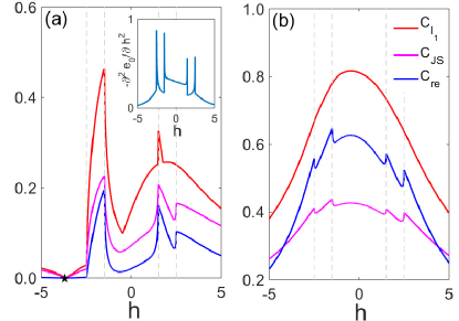
Figure 6: Quantum coherence measures on (a) odd bonds and (b) even bonds for increasing magnetic field $h$ with $J_{1}=1$, $J_{2}=4$, $J_{3}=2$, $\delta=0.5$. The legend shown in (b) is the same with (a). The symbol $\star$ marks the position of $h_{\star}=-3.647$. The dashed lines correspond to positions of $\pm|J_{3}\pm\delta|$. Inset in (a) shows the second-order derivative of the ground-state energy $e_{0}$.

In terms of the two-qubit $X$ state in Eq. (22), $\bar{D}_{i}(\rho_{ij})$ is identical to $C_{\rm re}(\rho_{ij})$. Without the loss of generality, we mainly use $C_{\rm re}(\rho)$ hereafter although it has two-fold implications in quantum correlations. Besides, the $l_{1}$ norm quantum coherence can be simplified to:

$$C_{l_{1}}(\rho) = \max\left\{\left|\langle\sigma_{i}^{x}\sigma_{j}^{x}\rangle\right|,\left|\langle\sigma_{i}^{y}\sigma_{j}^{y}\rangle\right|\right\}.$$ (29)

For our purposes, the correlation and coherence measures in the ground state of the quantum compass chain under an alternating transverse magnetic field for two spins are investigated in the following for comparison. Figures 6 and 7 display the results for the relative entropy, the $l_{1}$ norm quantum coherence and the JS divergence of two qubits in the ground state of the compass chain. We find $C_{l_{1}}(\rho)\geq C_{re}(\rho)$ holds, as was conjectured in Ref. Rana16 . The conjecture was proved only for the pure state and not yet proven for mixed state, and our findings indicate its validity.

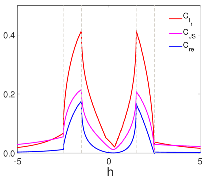
Figure 7: Quantum coherence measures of next nearest neighbor qubits for increasing magnetic field $h$ with $J_{1}=1$, $J_{2}=4$, $J_{3}=2$, $\delta=0.5$. The dashed lines mark the positions of $\pm|J_{3}\pm\delta|$.

Looking at the relative entropy, the $l_{1}$ norm quantum coherence and the JS divergence on the odd bonds presented in Fig. 6(a), three measures become zero simultaneously at $h_{\star}=-3.647$. The relative entropy shows a smooth local minimum at this special point, which is different from nonanalytical behaviors of its counterparts. The null point of coherence measures corresponds to a factoring point, where the intersite-correlators on the weak bonds $\langle\sigma^{x}_{2i-1}\sigma^{x}_{2i}\rangle$ and $\langle\sigma^{y}_{2i-1}\sigma^{y}_{2i}\rangle$ vanish, see Fig. 5(b). As a consequence, the density matrix (22) becomes diagonal in the orthogonal product bases. This factoring point is found to be $\delta$ independent, and such a accidental inflexion will be absent in the quantum coherence measures for the even bonds, see Fig. 6(b), and the next-nearest-neighboring qubits, see Fig. 7. One finds the quantum coherence on even bonds is larger than that on odd bonds, and the next-nearest neighbor coherence is a little smaller.

For $\delta=0$ the system undergoes a BKT phase transition, and the quantum coherence exhibits a local maximum; see Fig. 10(a) in Ref. You17 . For $\delta\neq 0$, the transitions for increasing $h$ belong to second-order phase transitions, as is verified in inset of Fig. 6(a). In this respect, we find that the coherence measures exhibit either a nonanalytical behavior or an extremum across QCPs, indicating sudden changes take place.

After a closer inspection we find the $l_{1}$ norm quantum coherence displays anomalies at QCPs $h_{c}=-J_{3}-\delta$, $\pm(J_{3}-\delta)$, but it misses the QCP at $h_{c}=J_{3}+\delta$. We also observe that there are superfluous kinks of the $l_{1}$ norm of coherence in regions around $h=0$, as shown in Figs. 6(a) and 7. The artificial turning points can be ascribed to the definition of $l_{1}$ norm quantum coherence in Eq. (1). Further, this norm does not exhibit any anomaly on the strong bonds, as shown in Fig. 6(b). From such a comparison one can find that relative entropy [Eq. (2)] can faithfully reproduce quantum criticality. Despite of their formal resemblances, the JS divergence and the $l_{1}$ norm quantum coherence, as different perspectives of quantum coherence, embody infidelity of density matrix and are insufficient to readout the locations of QCPs.

VI Discussion and summary

In this paper we consider a one-dimensional Hamiltonian with short-range interactions that includes three-site interactions and alternating magnetic fields. The one-dimensional quantum compass model is a paradigmatic scenario of quantum many-body physics, which is more subtle than the Ising model, and hence hosts richer phase diagrams. For a second-order quantum phase transition from a gapped Néel phase to a gapped paramagnetic phase, tools of quantum information theory can always be employed to characterize successfully the transition points. Usually achieving a complete and rigorous quantum-mechanical formulation of a many-body system as desired is obstructed by the complexity of quantum correlations in many-body states.

The spin chain in the present model is efficiently solvable using the standard Jordan-Wigner and Bogoliubov transformation techniques. Adopting the exact solvability we describe the phase diagram of the model as a function of its parameters. The perpendicular Zeeman field and and three-site interactions spoil the intermediate symmetry in the generic compass model, and thus they destroy the ground-state degeneracy of the quantum compass chain. The tunability of the staggered magnetic field entails the ground state can be among paramagnetic phase, dimer phase, and spin-liquid phases, in which the number of Fermi points falls into two categories. Except the multi-critical points, the phase transitions are of second order. The critical exponents can be extracted from low-energy spectra and gap scalings. Our investigations show a uniform magnetic field can drive the spin-liquid phase to the paramagnetic phase through the Berezinskii-Kosterlitz-Thouless transition, where a multi-critical point is found.

Since a quantum phase transition is driven by a purely quantum change in the many-body ground-state correlations, the notion of quantum coherence appears naturally and is suited to probe quantum criticality. To this end, we provide a study of associated exhibited quantum correlations in this model using a variety of quantum information theoretical measures, including the relative entropy and the $l_{1}$ norm quantum coherence along with the Jensen-Shannon divergence. These alternative frameworks of coherence theory stem mainly from different notions of incoherent (free) operations. It is thus desirable and interesting to find any interrelation between them.

We then compare the respective kinds of insights that they provide. We have found that the continuous phase transitions occurring in this model can be mostly faithfully detected by examining quantum information theoretical measures. We also discern some differences. The $l_{1}$ norm quantum coherence (defined as the sum of absolute values of off diagonals in the reduced density matrix) of odd bonds develops a singular behavior at non-criticality, which is caused by the absolute operator in the definition (29). Moreover, the $l_{1}$ norm quantum coherence of even bonds does not exhibit any anomaly across the critical points. A closer inspection reveals that the $l_{1}$ norm quantum coherence of even bond shows an inflection point and the transition point can be easily captured looking at its derivative with respect to $h$, which would display an extremum. On the contrary, the relative entropy and the Jensen-Shannon divergence show pronounced anomalies, either a sharp local maximum or a turning point. That is to say that they faithfully sense the rapid change of quantum correlation, resulting in a clear identification of quantum phase transitions. Also the $l_{1}$ norm quantum coherence and the Jensen-Shannon divergence become nonanalytical at exception points. Despite formal similarity, different measures of quantum coherence have their respective scope for detecting the quantum criticality. From such comparison, we believe that the relative entropy is more credible than others.

Summarizing, our results suggest that the diagonal entries of the density operator are indispensable to extract information across the quantum critical points. In other words, quantum phase transitions are cooperative phenomena where competing orders induce qualitative changes in many-body systems. The figures of merit of these measures might be crucial to the optimizing basis. Furthermore, we proposed an experimental scheme using superconducting quantum circuits to realize the compass chain with alternating magnetic fields.

Appendix A Diagonalization of the Hamiltonian

We are considering a 1D quantum compass model with the three-site (XZX$+$YZY) terms under staggered magnetic fields in Eq. (18), which can be rewritten as

$$\cal{H} = \sum_{i=1}^{N/2}\left(J_{1}\sigma_{2i-1}^{x}\sigma_{2i}^{x}+J_{2}\sigma_{2i}^{y}\sigma_{2i+1}^{y}\right)$$ (30)

$$+ \sum_{i=1}^{N/2}\left(h_{1}\,\hat{z}\cdot\vec{\sigma}_{2i-1}+h_{2}\,\hat{z}\cdot\vec{\sigma}_{2i}\right)$$

$$+ J_{3}\sum_{i=1}^{N}\left(\sigma^{x}_{i-1}\sigma^{z}_{i}\sigma^{x}_{i+1}+\sigma^{y}_{i-1}\sigma^{z}_{i}\sigma^{y}_{i+1}\right).$$

Here, $J_{1}$ and $J_{2}$ denote the coupling strength on odd and even bonds, respectively. $h_{1}$ and $h_{2}$ are the transverse external magnetic fields applied on odd and even sites, respectively. Finally, $J_{3}$ is the strength of (XZX$+$YZY)-type three-site exchange interactions.

First, we use a Jordan-Wigner transformation which maps explicitly a pseudo-spin model to a free-fermion system whose properties can always be computed efficiently as a function of system size EBarouch70 :

$$\sigma_{j}^{z} = 1-2c_{j}^{\dagger}c_{j},$$

$$\sigma_{j}^{x} = e^{i\phi_{j}}\left(c_{j}^{\dagger}+c_{j}\right),$$

$$\sigma_{j}^{y} = ie^{i\phi_{j}}\left(c_{j}^{\dagger}-c_{j}\right),$$ (31)

with $\phi_{j}$ being the phase accumulated by all earlier sites, i.e., $\phi_{j}=\pi\sum_{l<j}c_{l}^{\dagger}c_{l}$. Consequently, we have a simple bilinear form of Hamiltonian in terms of spinless fermions:

$$\cal{H}\! = \!\!\sum_{i=1}^{N/2}\!\left\{J_{1}\!\left[\left(c_{2i-1}^{\dagger}c_{2i}\!-c_{2i-1}c_{2i}^{\dagger}\right)\!+\!\left(c_{2i-1}^{\dagger}c_{2i}^{\dagger}\!-c_{2i-1}c_{2i}\right)\right]\right.$$ (32)

$$+ \left.J_{2}\left[\left(c_{2i}^{\dagger}c_{2i+1}-c_{2i}c_{2i+1}^{\dagger}\right)-\left(c_{2i}^{\dagger}c_{2i+1}^{\dagger}-c_{2i}c_{2i+1}\right)\right]\right.$$

$$+ \left.h_{1}\left(1-2c_{2i-1}^{\dagger}c_{2i-1}\right)+h_{2}\left(1-2c_{2i}^{\dagger}c_{2i}\right)\right.$$

$$+ \left.2J_{3}\left(c_{2j-1}^{\dagger}c_{2j+1}+c_{2j}^{\dagger}c_{2j+2}+{\rm H.c.}\right)\right\}.$$

The fermion version of this model corresponds to a dimerised $p$-wave superconductor, in which the electrons also generate next-nearest neighbor hopping. Such a two-component 1D Fermi gas on a lattice is realizable with current technology, for example on an optical lattice by using a Fermi-Bose mixture in the strong-coupling limit Lewenstein04 .

Following the standard Jordan-Wigner transformation, we rewrite the Hamiltonian in the momentum space by taking a discrete Fourier transformation for plural spin sites with the periodic boundary condition (PBC).

$$c_{2j-1}\!=\!\sqrt{\frac{2}{N}}\sum_{k}e^{-ikj}a_{k},\quad c_{2j}\!=\!\sqrt{\frac{2}{N}}\sum_{k}e^{-ikj}b_{k},$$ (33)

with discrete momenta as

$$k\!=\frac{2n\pi}{N},\quad n=-\left(\frac{N}{2}-1\!\right),-\left(\frac{N}{2}-3\!\right),\ldots,\left(\frac{N}{2}-1\!\right)\!.$$ (34)

Next the discrete Fourier transformation for plural spin sites is introduced for the PBC. The Hamiltonian takes the following form which is suitable to apply the Bogoliubov transformation:

$${\cal H} = \sum_{k}\left[T_{k}a_{k}^{\dagger}b_{k}-T_{k}^{*}a_{k}b_{k}^{\dagger}+T_{k}a_{k}^{\dagger}b_{-k}^{\dagger}-T_{k}^{*}a_{k}b_{-k}\right.$$

$$+ \left.F_{k}\left(a_{k}^{\dagger}a_{k}+b_{k}^{\dagger}b_{k}\right)+2\delta\left(a_{k}^{\dagger}a_{k}-b_{k}^{\dagger}b_{k}\right)+Nh\right],$$

where $T_{k}=J_{1}+J_{2}e^{ik}$ and $F_{k}=2J_{3}\cos k-2h$. After the Fourier transformation, $\cal{H}$ is then transformed into a sum of commuting Hamiltonians $\hat{H}_{k}$ describing a different $k$ mode each. Then we write the Hamiltonian in the BdG form in terms of Nambu spinors:

$$\cal{H} = \frac{1}{2}\sum_{k}\Upsilon_{k}^{\dagger}\hat{H}_{k}\Upsilon_{k},$$ (36)

where

$$\hat{H}_{k}=\left(\begin{array}[]{cccc}F_{k}+2\delta&T_{k}&0&T_{k}\\ T_{k}^{*}&F_{k}-2\delta&-T_{-k}&0\\ 0&-T_{-k}^{*}&-F_{k}-2\delta&-T_{k}\\ T_{k}^{*}&0&-T_{k}^{*}&-F_{k}+2\delta\end{array}\right),$$ (41)

and $\Upsilon_{k}^{\dagger}=(a_{k}^{\dagger},b_{k}^{\dagger},a_{-k},b_{-k})$. In momentum space, time reversal (TR) symmetry and particle-hole (PH) symmetry of the BdG Hamiltonian $\hat{H}_{k}$ are implemented by anti-unitary operators $T$ and $\mathbf{C}$. For spinless fermions TR operator $T$ is simply a complex conjugation $\cal{K}$ and operator $\mathbf{C}=\tau_{x}K$ as the PH transformation. The system Eq. (41) belongs to topological class $D$ with topological invariant $\mathbb{Z}_{2}$ in one dimension, which satisfies $\hat{H}(-k){\cal C}=-{\cal C}\hat{H}(k)$. Here ${\cal C}=\tau^{x}\otimes\sigma^{0}\cal{K}$, where $\tau^{x}$ and $\sigma^{0}$ are the Pauli matrices acting on PH space and spin space, respectively.

The diagonalized form of $\hat{H}_{k}$ can be achieved by a four-dimensional Bogoliubov transformation which connects the original operators $\{a_{k}^{\dagger},b_{k}^{\dagger},a_{-k},b_{-k}\}$, with two kind of quasiparticles, $\{\gamma_{k,1}^{\dagger},\gamma_{k,2}^{\dagger},\gamma_{-k,1},\gamma_{-k,2}\}$, as follows,

$$\left(\begin{array}[]{c}\gamma_{k,1}^{\dagger}\\ \gamma_{k,2}^{\dagger}\\ \gamma_{-k,1}\\ \gamma_{-k,2}\end{array}\right)=\hat{U}_{k}\left(\begin{array}[]{c}a_{k}^{\dagger}\\ b_{k}^{\dagger}\\ a_{-k}\\ b_{-k}\end{array}\right).$$ (50)

$\hat{H}_{k}$ is diagonalized by a unitary transformation (50),

$${\cal H}=\sum_{k}\Upsilon_{k}^{\dagger}\hat{U}_{k}\hat{U}_{k}^{\dagger}\hat{H}_{k}\hat{U}_{k}\hat{U}_{k}^{\dagger}\Upsilon_{k}=\sum_{k}\Upsilon_{k}^{\prime\dagger}D_{k}\Upsilon_{k}^{\prime}.\quad$$ (51)

The obtained four eigenenergies $\{\varepsilon_{k,j}\}$ ($j=1,\cdots,4$)

$$\varepsilon_{k,1(2)} = \sqrt{|T_{k}|^{2}+F_{k}^{2}}\pm\sqrt{|T_{k}|^{2}+4\delta^{2}},$$

$$\varepsilon_{k,4(3)} = -\sqrt{|T_{k}|^{2}+F_{k}^{2}}\mp\sqrt{|T_{k}|^{2}+4\delta^{2}},$$ (52)

in the diagonalized Hamiltonian matrix $D_{k}=\hat{U}_{k}^{\dagger}\hat{H}_{k}\hat{U}_{k}$ are the excitations in the artificially enlarged PH space where the positive (negative) ones denote the electron (hole) excitations. The ground state corresponds to the state in which all hole modes are occupied while the electron modes are vacant. The PH symmetry indicates here that $\gamma_{k,4}^{\dagger}=\gamma_{-k,1}$ and $\gamma_{k,3}^{\dagger}=\gamma_{-k,2}$. So the spectra consist of two branches of energies $\varepsilon_{k,j}$ (with $j=1,2$), and

$$\hat{H}_{k} = \frac{1}{2}\,\varepsilon_{k,1}\left(\gamma_{k,1}^{\dagger}\gamma_{k,1}-\gamma_{-k,1}\gamma_{-k,1}^{\dagger}\right)$$ (53)

$$+ \frac{1}{2}\,\varepsilon_{k,2}\left(\gamma_{k,2}^{\dagger}\gamma_{k,2}-\gamma_{-k,2}\gamma_{-k,2}^{\dagger}\right)$$

$$= \sum_{j=1}^{2}\,\varepsilon_{k,j}\left(\gamma_{k,j}^{\dagger}\gamma_{k,j}-\frac{1}{2}\right).$$

Two-point correlation functions for the real Hamiltonian Eq. (30) can be expressed as an expansion of Pfaffians using the Wick theorem,

$$\langle\sigma_{i}^{x}\sigma_{j}^{x}\rangle = \left|\begin{array}[]{c c c c}G_{-1}&G_{-2}&\cdot&G_{i-j}\\ G_{0}&G_{-1}&\cdot&G_{i-j+1}\\ \vdots&\vdots&\ddots&\vdots\\ G_{j-i-2}&G_{j-i-3}&\cdot&G_{-1}\end{array}\right|,$$ (58)

$$\langle\sigma_{i}^{y}\sigma_{j}^{y}\rangle = \left|\begin{array}[]{c c c c}G_{1}&G_{0}&\cdot&G_{i-j+2}\\ G_{2}&G_{1}&\cdot&G_{i-j+3}\\ \vdots&\vdots&\ddots&\vdots\\ G_{j-i}&G_{j-i-1}&\cdot&G_{1}\end{array}\right|,$$ (63)

$$\langle\sigma_{i}^{z}\sigma_{j}^{z}\rangle = \langle\sigma_{i}^{z}\rangle\langle\sigma_{j}^{z}\rangle-G_{j-i}G_{i-j},$$ (64)

where $G_{r}=\langle(c_{0}^{\dagger}-c_{0})(c_{r}^{\dagger}+c_{r})\rangle$ and $r=j-i$ represents the distance between the two sites in units of the lattice constant.

References

- (1) A. Streltsov, G. Adesso, and M. B. Plenio, Rev. Mod. Phys. 89, 041003 (2017).
- (2) A. Osterloh, L. Amico, G. Falci, and R. Fazio, Nature 416, 608 (2002).
- (3) H. Ollivier and W. H. Zurek, Phys. Rev. Lett. 88, 017901 (2001).
- (4) M. Nath Bera, A. Acín, M. Kuś, M. Mitchell, and M. Lewenstein, Rep. Prog. Phys. 80, 124001 (2017).
- (5) T. Baumgratz, M. Cramer, and M. B. Plenio, Phys. Rev. Lett. 113, 140401 (2014).
- (6) D. Girolami, Phys. Rev. Lett. 113, 170401 (2014).
- (7) T. R. Bromley, M. Cianciaruso, and G. Adesso, Phys. Rev. Lett. 114, 210401 (2015).
- (8) A. Streltsov, U. Singh, H. S. Dhar, M. N. Bera, and G. Adesso, Phys. Rev. Lett. 115, 020403 (2015).
- (9) E. Chitambar, A. Streltsov, S. Rana, M. N. Bera, G. Adesso, and M. Lewenstein, Phys. Rev. Lett. 116, 070402 (2016).
- (10) N. Killoran, F. E. S. Steinhoff, and M. B. Plenio, Phys. Rev. Lett. 116, 080402 (2016).
- (11) A. Winter and D. Yang, Phys. Rev. Lett. 116, 120404 (2016).
- (12) C. Napoli, T. R. Bromley, M. Cianciaruso, M. Piani, N. Johnston, and G. Adesso, Phys. Rev. Lett. 116, 150502 (2016).
- (13) E. Bagan, J. A. Bergou, S. S. Cottrell, and M. Hillery, Phys. Rev. Lett. 116, 160406 (2016).
- (14) J. Ma, B. Yadin, D. Girolami, V. Vedral, and M. Gu, Phys. Rev. Lett. 116, 160407 (2016).
- (15) A. Streltsov, E. Chitambar, S. Rana, M. N. Bera, A. Winter, and M. Lewenstein, Phys. Rev. Lett. 116, 240405 (2016).
- (16) E. Chitambar and M.-H. Hsieh, Phys. Rev. Lett. 117, 020402 (2016).
- (17) E. Chitambar and G. Gour, Phys. Rev. Lett. 117, 030401 (2016).
- (18) Zi-Wen Liu, X. Hu, and S. Lloyd, Phys. Rev. Lett. 118, 060502 (2017).
- (19) K. Bu, U. Singh, S.-M. Fei, A. K. Pati, and J. Wu, Phys. Rev. Lett. 119, 150405 (2017).
- (20) T. Theurer, N. Killoran, D. Egloff, and M. B. Plenio, Phys. Rev. Lett. 119, 230401 (2017).
- (21) Yi-Tao Wang, J.-S. Tang, Z.-Y. Wei, S. Yu, Zhi-Jin Ke, X.-Ye Xu, C.-F. Li, and G.-C. Guo, Phys. Rev. Lett. 118, 020403 (2017).
- (22) Da-J. Zhang, C. L. Liu, X.-D. Yu, and D. M. Tong, arXiv:1707.02966.
- (23) M.-L. Hu, X. Hu, J.-Ci Wang, Yi Peng, Yu-R. Zhang, and H. Fan, arXiv:1703.01852.
- (24) C. Radhakrishnan, M. Parthasarathy, S. Jambulingam, and T. Byrnes, Phys. Rev. Lett. 116, 150504 (2016).
- (25) S. Rana, P. Parashar, A. Winter, and M. Lewenstein, Phys. Rev. A 96, 052336 (2017).
- (26) H. Zhu, M. Hayashi, and L. Chen, Phys. Rev. A 97, 022342 (2018).
- (27) S. Rana, P. Parashar, and M. Lewenstein, Phys. Rev. A 93, 012110 (2016).
- (28) A. P. Majtey, P. W. Lamberti, and D. P. Prato, Phys. Rev. A 72, 052310 (2005).
- (29) A. L. Malvezzi, G. Karpat, B. Çakmak, F. F. Fanchini, T. Debarba, and R. O. Vianna, Phys. Rev. B 93, 184428 (2016).
- (30) W.-L. You, A. M. Oleś, and P. Horsch, New J. Phys. 17, 083009 (2015); W.-L. You, P. Horsch, and A. M. Oleś, Phys. Rev. B 92, 054423 (2015).
- (31) N. Blanc, J. Trinh, L. Dong, X. Bai, A. A. Aczel, M. Mourigal, L. Balents, T. Siegrist, and A. P. Ramirez, Nat. Phys. 14, 273 (2018).
- (32) F. Trousselet, A. M. Oleś, and P. Horsch, Europhys. Lett. 91, 40005 (2010); Phys. Rev. B 86, 134412 (2012).
- (33) W. Brzezicki, J. Dziarmaga, and A. M. Oleś, Phys. Rev. B 75, 134415 (2007); W. Brzezicki and A. M. Oleś, Acta Phys. Polon. A 115, 162 (2009).
- (34) W.-L. You, Eur. Phys. J. B 85, 83 (2012).
- (35) R. Jafari and H. Johannesson, Phys. Rev. Lett. 118, 015701 (2017).
- (36) W.-L. You, G.-H. Liu, P. Horsch, and A. M. Oleś, Phys. Rev. B 90, 094413 (2014).
- (37) Y.-C. Qiu, Q.-Q. Wu, and W.-L. You, J. Phys.: Condens. Matter 28, 496001 (2016).
- (38) I. Affleck and M. Oshikawa, Phys. Rev. B 60, 1038 (1999); M. Oshikawa and I. Affleck, Phys. Rev. Lett. 79, 2883 (1997).
- (39) A. Fledderjohann, C. Gerhardt, K. H. Mütter, A. Schmitt, and M. Karbach, Phys. Rev. B 54, 7168 (1996).
- (40) J. Z. Zhao, X. Q. Wang, T. Xiang, Z. B. Su, and L. Yu, Phys. Rev. Lett. 90, 207204 (2003).
- (41) M. Kenzelmann, Y. Chen, C. Broholm, D. H. Reich, and Y. Qiu, Phys. Rev. Lett. 93, 017204 (2004).
- (42) M. Kohgi, K. Iwasa, J.-M. Mignot, B. Fåk, P. Gegenwart, M. Lang, A. Ochiai, H. Aoki, and T. Suzuki, Phys. Rev. Lett. 86, 2439 (2001).
- (43) W. P. Su, J. R. Schrieffer, and A. J. Heeger, Phys. Rev. Lett. 42, 1698 (1979); Phys. Rev. B 22, 2099 (1980).
- (44) J. D. Sau, R. M. Lutchyn, S. Tewari, and S. Das Sarma, Phys. Rev. Lett. 104, 040502 (2010).
- (45) J. Alicea, Phys. Rev. B 81, 125318 (2010).
- (46) A. Das, Y. Ronen, Y. Most, Y. Oreg, M. Heiblum, and H. Shtrikman, Nat. Phys. 8, 887 (2012).
- (47) S. Nadj-Perge, I. K. Drozdov, J. Li, H. Chen, S. Jeon, J. Seo, A. H. MacDonald, B. A. Bernevig, and A. Yazdani, Science 346, 602 (2014).
- (48) R. Feyerherm, S. Abens, D. Günther, T. Ishida, M. Meißner, M. Meschke, T. Nogami, and M. Steiner, J. Phys.: Condens. Matter 12, 8495 (2000).
- (49) G. Wendin and V. S. Shumeiko, arXiv:cond-mat/0508729.
- (50) J. Q. You and F. Nori, Phys. Today 58, 42 (2005).
- (51) M. H. Devoret and R. J. Schoelkopf, Science 339, 1169 (2013).
- (52) J. Q. You, X.-F. Shi, X. Hu, and F. Nori, Phys. Rev. B 81, 014505 (2010).
- (53) U. L. Heras, A. Mezzacapo, L. Lamata, S. Filipp, A. Wallraff, and E. Solano, Phys. Rev. Lett. 112, 200501 (2014).
- (54) R. Barends, L. Lamata, J. Kelly, L. García-Álvarez, A. G. Fowler, A. Megrant, E. Jeffrey, T. C. White, D. Sank, J. Y. Mutus, B. Campbell, Y. Chen, Z. Chen, B. Chiaro, A. Dunsworth, I.-C. Hoi, C. Neill, P. J. J. O’Malley, C. Quintana, P. Roushan, A. Vainsencher, J. Wenner, E. Solano, and J. M. Martinis, Nat. Commun. 6, 7654 (2015).
- (55) R. Barends, A. Shabani, L. Lamata, J. Kelly, A. Mezzacapo, U. L. Heras, R. Babbush, A. G. Fowler, B. Campbell, Y. Chen, Z. Chen, B. Chiaro, A. Dunsworth, E. Jeffrey, E. Lucero, A. Megrant, J. Y. Mutus, M. Neeley, C. Neill, P. J. J. O’Malley, C. Quintana, P. Roushan, D. Sank, A. Vainsencher, J. Wenner, T. C. White, E. Solano, H. Neven, and J. M. Martinis, Nature 534, 222 (2016).
- (56) Y. Wang, W.-L. You, M. Liu, Yu-Li Dong, H.-G. Luo, G. Romero, and J. Q. You, New J. Phys. 20, 053061 (2018).
- (57) J. Q. You, J. S. Tsai, and F. Nori, Phys. Rev. Lett. 89, 197902 (2002).
- (58) Y. Makhlin, G. Schön, and A. Shnirman, Nature (London) 398, 305 (1999); Rev. Mod. Phys. 73, 357 (2001).
- (59) Y. A. Pashkin, T. Yamamoto, O. Astafiev, Y. Nakamura, D. V. Averin, and J. S. Tsai, Nature (London) 421, 823 (2003).
- (60) W.-L. You, C.-J. Zhang, W. Ni, M. Gong, and A. M. Oleś, Phys. Rev. B 95, 224404 (2017).
- (61) N. Bergeal, R. Vijay, V. E. Manucharyan, I. Siddiqi, R. J. Schoelkopf, S. M. Girvin, and M. H. Devoret, Nat. Phys. 6, 296 (2010).
- (62) N. Chancellor, S. Zohren, and P. A. Warburton, NPJ Quantum Inf. 3, 21 (2017).
- (63) M. Leib, P. Zoller, and W. Lechner, Quantum Sci. Technol. 1, 015008 (2016).
- (64) J. Zhang, X. Peng, and D. Suter, Phys. Rev. A 73, 062325 (2006).
- (65) H. P. Buchler, A. Micheli and P. Zoller, Nat. Phys. 3, 726 (2007).
- (66) M. Sameti, A. Potoc̆nik, D. E. Browne, A. Wallraff, and M. J. Hartmann, Phys. Rev. A 95, 042330 (2017).
- (67) M. Marvian, T. A. Brun, and D. A. Lidar, Phys. Rev. A 96, 052328 (2017).
- (68) T. O. Puel, P. D. Sacramento, and M. A. Continentino, J. Phys.: Condens. Matter 27, 422002 (2015).
- (69) S. A. Yang, H. Pan, and F. Zhang, Phys. Rev. Lett. 113, 046401 (2014).
- (70) M. Neupane, I. Belopolski, M. M. Hosen, D. S. Sanchez, R. Sankar, M. Szlawska, S.-Y. Xu, K. Dimitri, N. Dhakal, P. Maldonado, P. M. Oppeneer, D. Kaczorowski, F. Chou, M. Z. Hasan, and T. Durakiewicz, Phys. Rev. B 93, 201104(R) (2016).
- (71) Y. Cao, S.-H. Zou, X.-J. Liu, S. Yi, G.-L. Long, and H. Hu, Phys. Rev. Lett. 113, 115302 (2014).
- (72) O. Pavlosiuk, D. Kaczorowski, and P. Wiśniewski, Sci. Rep. B 5, 9158 (2015).
- (73) W. Brzezicki, A. M. Oleś, and M. Cuoco, Phys. Rev. B 95, 140506(R) (2017).
- (74) W. Brzezicki and M. Cuoco, Phys. Rev. B 97, 064513 (2018).
- (75) Ke-Wei Sun and Qing-Hu Chen, Phys. Rev. B 80, 174417 (2009).
- (76) M. Motamedifar, S. Mahdavifar, S. F. Shayesteh, and S. Nemati, Phys. Scr. 88, 015003 (2013).
- (77) Y. Kono, T. Sakakibara, C. P. Aoyama, C. Hotta, M. M. Turnbull, C. P. Landee, and Y. Takano, Phys. Rev. Lett. 114, 037202 (2015).
- (78) E. Barouch and B. M. McCoy, Phys. Rev. A 2, 1075 (1970); 3, 786 (1971).
- (79) T. J. Osborne and M. A. Nielsen, Phys. Rev. A 66, 032110 (2002).
- (80) Zi-Wen Liu, R. Takagi, and S. Lloyd, arXiv:1708.09076.
- (81) M. Lewenstein, L. Santos, M. A. Baranov, and H. Fehrmann, Phys. Rev. Lett. 92, 050401 (2004).