Reduction of multivariate mixtures and its applications
Abstract.
We consider fast deterministic algorithms to identify the “best” linearly independent terms in multivariate mixtures and use them to compute, up to a user-selected accuracy, an equivalent representation with fewer terms. One algorithm employs a pivoted Cholesky decomposition of the Gram matrix constructed from the terms of the mixture to select what we call skeleton terms and the other uses orthogonalization for the same purpose. Importantly, the multivariate mixtures do not have to be a separated representation of a function. Both algorithms require operations, where is the initial number of terms in the multivariate mixture, is the number of selected linearly independent terms, and is the cost of computing the inner product between two terms of a mixture in variables. For general Gaussian mixtures since we need to diagonalize a matrix, whereas for separated representations (there is no need for diagonalization). Due to conditioning issues, the resulting accuracy is limited to about one half of the available significant digits for both algorithms. We also describe an alternative algorithm that is capable of achieving higher accuracy but is only applicable in low dimensions or to multivariate mixtures in separated form.
We describe a number of initial applications of these algorithms to solve partial differential and integral equations and to address several problems in data science. For data science applications in high dimensions, we consider the kernel density estimation (KDE) approach for constructing a probability density function (PDF) of a cloud of points, a far-field kernel summation method and the construction of equivalent sources for non-oscillatory kernels (used in both, computational physics and data science) and, finally, show how to use the new algorithm to produce seeds for subdividing a cloud of points into groups.
1. Introduction
We present (what we call) reduction algorithms for computing with multivariate mixtures that allow us to obtain solutions of PDEs in high dimensions as well as to address several problems in data science. We describe a new approach for solving partial differential and integral equations in a functional form, consider a far-field kernel summation method and the construction of equivalent sources for non-oscillatory kernels. As an illustration of data science applications, we present examples of using these reduction algorithms for kernel density estimation (KDE) to construct a probability density function (PDF) of a cloud of points and to generate seeds for subdividing a cloud of points into groups.
We use the well-known pivoted Cholesky factorization111Pivoted Cholesky decomposition of the Gram matrix was used by Martin Mohlenkamp (Ohio University) and G.B. for the reduction of the number of terms in separated representations (see comments in [14]). as well as a version of modified Gram-Schmidt orthogonalization to identify the “best” linearly independent terms from a collection of functions. The renewed interest in this problem is due to two observations: (i) the approach can be used for more general multivariate mixtures than the separated representations in [8, 9] and (ii) multivariate Gaussian mixtures can achieve any target accuracy when approximating functions since a multiresolution analysis can employ a Gaussian as an approximate scaling function [13]. The first observation makes our approach so far the only choice for reduction of general multivariate mixtures while the second assures that a multivariate Gaussian mixture (and its modifications that e.g. include polynomial factors) is sufficient to represent an arbitrary function while allowing us to exploit the fact that integrals involving Gaussian mixtures can be evaluated explicitly. We expand further on these observations below.
We consider multivariate functions that can be approximated via a linear combination of multivariate atoms,
| (1.1) |
such that the inner product between the atoms,
| (1.2) |
can be computed efficiently. We normalize the atoms so that they have unit -norm
A particularly important example are multivariate Gaussian atoms yielding a multivariate Gaussian mixture. In this case the atoms are
where is the standard multivariate Gaussian distribution with mean , symmetric positive definite covariance matrix , and . Already in early quantum chemistry computations, Gaussian mixtures were used because integrals involving them can be computed explicitly (see e.g. [17, 34, 43]). Indeed, integrals with Gaussians (and (1.2) in particular), can be evaluated explicitly in any dimension. Multivariate Gaussian mixtures (as well as other multivariate atoms) are used within the Radial Basis Functions (RBF) approach (see e.g. [22] and references therein). A method for approximating smooth functions via Gaussians and a number of its applications have been developed in [36].
As was demonstrated previously, a number of key operators of mathematical physics can be efficiently represented via Gaussians leading to their separated representations (see e.g. [8, 9, 11, 12, 6]) and, as a consequence, to practical algorithms (see [28, 46, 47, 27]). Importantly, as it was demonstrated recently, for any finite but arbitrary accuracy a Gaussian can serve as a scaling function of an approximate multiresolution analysis [13].
These considerations combined with algorithms of this paper to reduce the number of terms in (1.1) suggest a new type of numerical algorithms. The basic idea of such algorithms is simple: in the process of iteratively solving equations, we represent both operators and functions via Gaussians and, at each iteration step, compute the required integrals explicitly. The difficulty of this approach is then how to deal with a rapid proliferation of terms in the resulting Gaussian mixtures. For example, if an integral involves three Gaussian mixtures with terms each, the resulting Gaussian mixture has terms. However, in most practical applications most of these terms are close to be linearly dependent and, thus, to represent the result, we only need a fast algorithm to find the “best” linearly independent subset of the terms. We describe (what we call) reduction algorithms to maintain a reasonable number of terms in intermediate computations when using these representations.
The multivariate mixtures that we consider (and construct algorithms for) can be significantly more general than the separated representations introduced in [8, 9] for the purpose of computing in higher dimensions by avoiding “the curse of dimensionality”. Recall that a separated representation is a natural extension of the usual separation of variables as we seek an approximation
| (1.4) |
where the functions are normalized by the standard -norm, and are referred to as -values. In this approximation the functions are not fixed in advance but are optimized as to achieve the accuracy goal with (ideally) a minimal separation rank . Importantly, a separated representation is not a projection onto a subspace, but rather a nonlinear method to track a function in a high-dimensional space while using a small number of parameters. The key to obtaining useful separated representations is to use the Alternating Least Squares (ALS) algorithm to reduce the separation rank while maintaining an acceptable error. ALS is one of the key tools in numerical multilinear algebra and was originally introduced for data fitting as PARAFAC model (PARAllel FACtor analysis) [29] and CANDECOMP (Canonical Tensor Decomposition) [19]. ALS has been used extensively in data analysis of (mostly) three-way arrays (see e.g. the reviews [44, 18], [31] and references therein). We note that any discretization of in (1.4) leads to a -dimensional tensor yielding a canonical tensor decomposition of separation rank ,
| (1.5) |
where the -values are chosen so that each vector has unit Frobenius norm for all . However, the ALS algorithm relies heavily on the separated form (1.4-1.5) and is not available for general multivariate mixtures.
In this paper we detail and use algorithms to reduce the number of terms in multivariate mixtures that do not necessarily admit a separated representation. In spite their accuracy limitations, these algorithms have several advantages as their complexity depends mildly on the number of variables, the dimension . The “mild” dependence should be understood in the context of the “curse of dimensionality” arising when fast algorithms in low dimensions are extended to high dimensions in a straightforward manner. Fast reduction algorithms of this paper require operations, where is the initial number of terms in a multivariate mixture, is the number of selected terms and is the cost of computing the inner product between two terms of the mixture. We also describe an algorithm capable of achieving higher accuracy by avoiding the loss of precision due to conditioning issues but which currently is only applicable in low dimensions or to multivariate mixtures in separated form.
We start by describing reduction algorithms in Section 2. We then present several examples of using a reduction algorithm for solving equations in Section 3. In Section 4 we show how to apply our approach to construct the PDF for a cloud of points in high dimensions using the KDE approach. We then turn to far-field summation in high dimensions in Section 5 and demonstrate how to use a reduction algorithm in this problem and for the problem of finding equivalent sources. We also describe how to use a reduction algorithm for splitting a cloud of points into groups (potentially in a hierarchical manner) and briefly mention properties of such subdivisions. Conclusions are presented in Section 6 and some key identities for multivariate Gaussians in the Appendix.
2. Reduction Algorithms
In this section we describe fast deterministic algorithms to reduce the number of terms of a linear combination of multivariate functions of variables by selecting the “best” subset of these functions that can, within a target accuracy, approximate the rest of them. The first algorithm is based on a pivoted Cholesky decomposition of the Gram matrix of the terms of the multivariate mixture; we assume that the entries of this matrix, i.e. the inner product of these functions, can be computed efficiently. This algorithm was mentioned in the discussion of tensor interpolative decomposition (tensor ID) of the canonical tensor representation in [14]. Due to the use of a Gram matrix, the accuracy of this approach is limited to about one half of the available significant digits (e.g. when using double precision arithmetic). The second algorithm is based on a pivoted modified Gram-Schmidt orthogonalization and achieves the same accuracy (due to conditioning issues) as the first algorithm. Nevertheless, these algorithms appear advantageous in high dimensions since their complexities depend mildly on dimension and, if desired, full accuracy can be restored by performing some evaluations in higher precision. We also describe an alternative approach that achieves full precision, but so far is limited to low dimensions or mixtures in separated form. For this alternative reduction algorithm, we need access to the Fourier transform of the functions in the mixture. Since the Fourier transform is readily available for Gaussian atoms, we present this algorithm for the case of Gaussian mixtures and note that it can be used for any functional form that allows a rapid computation of the integrals involved.
2.1. Cholesky reduction
We start with a linear combination of atoms of the form
| (2.1) |
and, within a user-selected accuracy , seek a representation of the same form but with fewer terms. More precisely, we look for a partition of indices where and , and new coefficients , such that the function
| (2.2) |
approximates ,
| (2.3) |
We present an algorithm based on a partial, pivoted Cholesky decomposition of the Gram matrix constructed using the atoms in (2.1) and provide an estimate for the error in (2.3).
By analogy with the matrix Interpolative Decomposition (matrix-ID) (see e.g. [26]), we call the subset the skeleton terms and the residual terms. In order to identify the “best” subset of linear independent terms, we compute a pivoted Cholesky decomposition of the Gram matrix of the atoms of the multivariate mixture in (2.1). If the number of terms, , is large then the cost of the full Cholesky decomposition is prohibitive. However, we show that we can terminate the Cholesky decomposition once the pivots are below a selected threshold. As a result, the complexity of the algorithm is , where is the initial number of terms, is the number of selected (skeleton) terms and is the cost of computing the inner product between two terms of a mixture in variables. In fact, the final result will be the same as if we were to perform the full decomposition and then keep only the significant terms. This property is a consequence of the following lemma that can be found in e.g. [30, p.434, problem 7.1.P1].
Lemma 1.
Let be positive semi-definite and self-adjoint, i.e. and for any . Then its diagonal entries are non-negative and the entries of satisfy
| (2.4) |
In particular, assuming that the first diagonal entries are in descending order and are greater or equal than the remaining diagonal entries,
we have
| (2.5) |
Proof.
Let be the standard basis vectors, that is, . The diagonal entries are non-negative since, for any index , . We now use the same approach to estimate the size of an off-diagonal entry . For the vector we have
| (2.6) |
Setting
in (2.6), we obtain
Thus, we arrive at
| (2.7) |
For the second part of the lemma, selecting implies that and, thus, (2.5) follows from the last inequality in (2.7). ∎
Lemma 1 implies
Corollary 2.
Let be a self-adjoint positive semi-definite matrix such that its Cholesky decomposition has monotonically decaying diagonal entries. If we write its Cholesky decomposition as
where is an lower triangular matrix with the smallest diagonal entry , then a partial Cholesky decomposition is of the form
where all entries of the matrix are less than .
Proof.
After applying steps of Cholesky decomposition, the matrix does not change in the consecutive steps. The remaining matrix is self-adjoint positive semi-definite and, due to the decay of the pivots, all of its diagonal entries are less than . Using Lemma 1, we conclude that all entries of are less than . ∎
Let us organize the collection of atoms in (2.1) as
We can view as a matrix with a gigantic number of rows resulting from a discretization of the argument . If we replace operations that require row-wise summation by the inner product between the atoms, then we can (and do) use matrix notation in the sequel. Without loss of generality, to simplify notation, we assume that the first atoms in form the skeleton, that is, , where denotes the skeleton atoms and the non-skeleton atoms.
Given the vector of coefficients in (2.1), we want to find new coefficients to approximate by
| (2.8) |
and estimate the error of the approximation. Note that we identify and .
We first seek an approximation of all atoms via the skeleton atoms,
Selecting the coefficients as the solutions of the least squares problem, satisfy the normal equations,
| (2.9) |
Introducing the matrix , we write (2.9) as
| (2.10) |
and observe that , where is the identity matrix and , an matrix, which satisfies
| (2.11) |
Setting
or
we obtain from (2.10) that the coefficients solve the system of normal equations
| (2.12) |
Theorem 3.
Let the Gram matrix ,
be such that its partial Cholesky decomposition has monotonically decaying pivots and is of the form
where is an lower triangular matrix with the smallest diagonal entry . If the coefficients of the skeleton terms are computed via (2.12), then the difference between in (2.1) and its approximation (2.8) can be estimated as
| (2.13) |
Proof.
We have
| (2.14) |
where the coefficient matrix solves the normal equations (2.10) and, therefore,
| (2.15) |
as well as
| (2.16) |
Using (2.15), we obtain
| (2.17) |
and proceed to compute . We have and , so that
Thus, we have
and, using (2.16), arrive at
| (2.18) |
Equating the two expressions of the Gram matrix in the statement of the Theorem,
we obtain that
| (2.19) |
| (2.20) |
and
| (2.21) |
We observe that from (2.11) using (2.19) and (2.20), we arrive at
| (2.22) |
Next we show that the non-zero block of the matrix in the right hand side of (2.18) coincides with . Using (2.20) and (2.22), we have
where we used that is non-singular. Hence, combining the last identity with (2.21), we obtain
| (2.23) |
By (2.14), (2.17) , (2.18), and (2.23) we obtain
Using Corollary 2, we estimate by its Frobenius norm,
which yields the desired estimate (2.13). ∎
Remark 4.
The estimate (2.13) is tighter than the one obtained in [14, Theorem 3.1] since the dependence on the number of terms is instead of . Yet, the estimate is still pessimistic since is usually significantly smaller than the Frobenius norm . In practice, for in the range , we did not observe the reduction of accuracy suggested by the factor .
In Table 1 we present pseudo-code for the reduction Algorithm 1. Note that this algorithm is dimension independent except for the cost of computing the inner product which we always assume to be reasonable by a judicious choice of the functions in the mixture. As a consequence of Theorem 3 and Lemma 1, it is sufficient to generate only entries of the Cholesky decomposition of the Gram matrix which requires operations, where is the cost of computing the inner product between two terms of a mixture. Therefore, the overall computational cost of Algorithm 1 is operations (see Table 2 for some examples). For a general Gaussian mixture is proportional to since we need to diagonalize a matrix in order to evaluate the explicit expression for the inner product in Appendix 7.0.4 whereas, for separated representations, no diagonalization is needed so that .
Inputs: Atoms and coefficients in the representation of and error tolerance, , . We assume that a subroutine to compute the inner product is available.
Outputs: A pivot vector , where contains indices of skeleton terms and indices of terms being removed from the final representation and the coefficients , such that due to Theorem 3.
Stage 1: Pivoted Cholesky decomposition of the Gram matrix.
Initialization.
We maintain the diagonal of the Cholesky factor separately and initialize it as (since all atoms have unit -norm).
Set and initialize a pivot vector as .
for
-
(1)
Find the largest element of the diagonal and its index
if goto Stage 2 -
(2)
Swap indices and in the pivot vector .
-
(3)
Set the diagonal element of the matrix
for
end
update:
end
Stage 2: Find new coefficients
-
(1)
Form a vector such that its -th element is the inner product of and
for
end -
(2)
Solve the linear system , where and using forward and backward substitution.
-
(3)
Add the original coefficients of the skeleton terms to to get the new coefficients
for
end
2.2. Reduction via a rank-revealing modified Gram-Schmidt algorithm
For ordinary matrices, Rank Revealing QR (RRQR) algorithms (see e.g. [21, 25] and references therein) select a set of linear independent columns that one can use to represent the other columns (within a certain accuracy). All matrix RRQR algorithms routinely use vector addition whereas, in our problem, the sum of two or more terms of multivariate mixture does not simplify and, therefore, a sum must to be maintained as a linear combination. Moreover, as far as we know, there is no analogue of the Householder reflection or Givens rotation (as tools for orthogonalization) unless we discretize the argument of the terms (note that for reduction in low dimensions we use a discretization of the Fourier transform of the terms of the mixture as described in Section 2.3). As long as we rely on the rapid evaluation of inner products, the reduction algorithm mimics the modified Gram-Schmidt (MGS) orthogonalization with the caveat that the sum of terms is maintained as a linear combination. Unfortunately, this algorithm (even for ordinary matrices) loses one half of significant digits (see [15] and discussion in [24, Section 5.2.9]) as does Algorithm 1 (it remains an open question if there exists a modification of MGS for our problem that maintains full accuracy). As we show below, the reduction algorithm via orthogonalization for multivariate mixtures has formal complexity , which is somewhat worse than the complexity of the reduction via Cholesky decomposition. However, since in a typical reduction , such algorithm can be considered to be of the same complexity as Algorithm 1.
To introduce notation, we consider a set of multivariate atoms and write
| (2.24) | ||||||
where the functions are orthogonal, are orthonormal, and
We can also rewrite (2.24) as
| (2.25) | ||||
where and , . We can also consider a set of coefficients , such that
To compute the coefficients in (2.25) and in (2.2), we need to evaluate the inner product between the multivariate atoms and which we denote as .
In order to estimate the computational cost, let us assume that the first steps have been accomplished so that the coefficients , , and in (2.25), the coefficients , in (2.2), the norms of , as well as the partial Gram matrix , , and are already available. We then select the term, , with the largest norm which we then swap to become the term with index . For simplicity of indexing we assume that such term was already in the position . Thus, our pivoting strategy uses a greedy algorithm by selecting terms with the largest norm (we note that alternative pivoting strategies may be possible but we do not explore them here).
Note that the norms , do not change in the steps that follow. At the -th step, we first need to compute the coefficients in , such that
as in (2.2). Since the norm is available we use (2.24) to evaluate
and, therefore, obtain
| (2.27) |
Computing the coefficients take operations at this step. Next, we compute the coefficients in (2.25) and update the term by subtracting and evaluate the resulting norms for . Specifically, for , we compute and
| (2.28) |
We update the norm of as follows,
where we used (2.28). At this step, computing , (2.28) and (2.2) are performed for each index so that it requires operations, where is the cost of computing the inner product between two terms of the mixture.
Once the skeleton terms are identified in the process of orthogonalization, we compute the coefficients of the new representation of the multivariate mixture via these terms, i.e. approximate as . Using the fact that for
we compute
so that
| (2.30) |
If the number of skeleton terms is then, combining complexity estimates for all steps, the resulting algorithm has a complexity . Since this algorithm is designed to be used when , we conclude that the overall cost is . Pseudo-code for this reduction algorithm is presented as Algorithm 2.
Inputs: Atoms and coefficients in the representation of and error tolerance, , . We assume that a subroutine to compute the inner product is available.
Outputs: The pivot vector , where contains indices of skeleton terms and indices of terms being removed from the final representation and the coefficients , such that
Stage 1: Pivoted MGS applied to the atoms
Set for . Note that, initially, all norms since all atoms have unit -norm.
Set rank and initialize a pivot vector as .
for
-
(1)
Find the largest norm and its index
if goto Stage 2 -
(2)
Swap indices and in the pivot vector .
-
(3)
set
for
end
for
update
end
update:
end
Stage 2: Find new coefficients , .
Compute new coefficients , .
2.3. Alternative reduction algorithms
Using Algorithm 1 or 2, half of the significant digits are lost due to poor conditioning (see examples in [14] and [40]). In order to identify “best” linear independent terms we can design a matrix with a better condition number if instead of the functions of the mixture we use a “dual” family for computing inner products. In the case of Gaussians (which are well localized), a natural set of such “dual” functions are exponentials with purely imaginary exponents (which are global functions); computing the inner product with them reduces to computing their Fourier transform. Therefore, as representatives of Gaussian atoms we can then use frequency vectors, i.e. samples of their Fourier transforms. Such sampling strategy should be sufficient to differentiate between all Gaussian atoms; it is fairly straightforward to achieve this in low dimensions or if the functions admit a separated representation. Currently, we do not know how to do it efficiently in high dimensions. Naively it appears to require the construction of a sample matrix with entries and additional work is required to understand how to lower this complexity. Alternatively, in dimensions it is sufficient to use samples if we were to use the straightforward generalization of the algorithm in dimension described below. In all cases, the last step in this approach is to compute the matrix ID of the sample matrix.
We present a deterministic algorithm in dimension and note that its extension to functions in separated form in high dimensions can follow the approach in [14]. We consider a univariate Gaussian mixture
| (2.31) |
where
and seek the best linear independent subset as in (2.2). Defining the Fourier transform of as
we obtain
We set the highest frequency of as
such that for and . We also set the lowest frequency , a positive value obtained experimentally. We then sample the interval using frequencies equally spaced on a logarithmic scale,
where is the number of samples. We choose , where is the expected final number of terms. In our setup, the column
serves as a representative of the Gaussian . In this way, we reduce the problem to that of using the matrix ID. Specifically, given frequencies , we construct a sample matrix ,
and compute its matrix ID (see e.g. [26]). We obtain a partition of indices where and denote the skeleton and residual terms respectively. We also obtain a matrix such that
where is a matrix that satisfies . We then compute the new coefficients as
and use them to approximate
The accuracy of this approximation appears to be the same as the accuracy of matrix ID. Unfortunately, for multivariate Gaussian atoms, the size of the matrix appears to grow too fast with the dimension (except in the case of separated representations where such dependence is linear). While our approach via frequency vectors can be extended in a straightforward manner to dimensions , it is of interest to construct an algorithm yielding high accuracy approximations in higher dimensions.
Inputs: Atoms and coefficients in the representation of , number of frequencies samples , and error tolerance . We assume that a subroutine to compute the Fourier transform is available.
Outputs: an index set , where contains indices of skeleton terms and contains indices of terms being removed from the final representation, and coefficients , such that with accuracy of the matrix ID.
-
(1)
set and compute where .
-
(2)
initialize .
-
(3)
construct matrix such that .
-
(4)
compute a matrix ID of to obtain a index partition and a matrix such that
-
(5)
compute new coefficients via , for .
2.4. Timings and comparisons
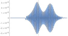
We compare the performance of Algorithms 1, 2 and 3 in dimension by considering a univariate Gaussian mixture of the form (2.31). We choose , and sample , and from uniform distributions , , and , respectively. We apply Algorithms 1, 2 and 3 to reduce the number of terms in the Gaussian mixture and display the original function and the errors of the resulting approximations in Figure 2.1.
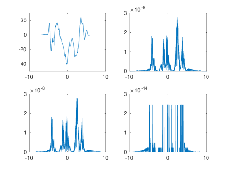
We run this experiment with different accuracy thresholds and display the resulting number of skeleton terms obtained by these algorithms in Table 1 (we use Algorithms 1 and 2 implemented in quadruple precision to make comparison possible for higher accuracies). We observe that the number of skeleton terms obtained by these algorithms differs only slightly (this difference is irrelevant for intended applications).
| Requested | Alg. 1 | Actual | Alg. 2 | Actual | Alg. 3 | Actual |
|---|---|---|---|---|---|---|
| accuracy | accuracy | accuracy | accuracy | |||
We also time Algorithm 1 (implemented in double precision) and examine its scaling as a function of the number of initial terms and the number of skeleton terms in dimensions and . In this test we fix the initial number of terms and vary the number of skeleton terms and vice versa. The resulting representation may not achieve a particular accuracy, but our the goal here is to see how Algorithm 1 scales in and . We consider a Gaussian mixture with parameters and sampled from uniform distributions and , respectively, and set matrices , where is a random unitary matrix and is a diagonal matrix with positive entries sampled from the uniform distribution . We report dimensions , the number of initial terms , the number of skeleton terms and the running time in seconds in Table 2. We implemented all algorithms in Fortran90 and compile them with Intel Fortran Compiler version 18.0.3. The computations are performed on a single core (without parallelization) using Intel i7-6700 CPU @3.4 GHz on a 64-bit Linux workstation with 64 GB of RAM.
| Fixed | Fixed | Fixed | Fixed | ||||
|---|---|---|---|---|---|---|---|
2.5. Applications of reduction algorithms
In the following sections, we present several examples of application of reduction algorithms in both low and high dimensions. In Section 3 we represent solutions of differential and integral equations in a functional form and adaptively solve these equations. We start with the free space Poisson’s equation with non-separable right hand side and then present an example of solving an elliptic problem with variable coefficients; we consider both examples in dimensions through . In Section 4 we first use our algorithm in dimension to construct an efficient representation of the PDF of a cloud of points via kernel density estimation and compare it with results obtained via the usual approach. We then present an example of constructing PDFs in high dimensions. Finally, we turn to kernel summation methods in high dimensions in Section 5, consider far-field evaluation in such computations and explore the problem of constructing equivalent sources in a similar setup. We also illustrate how a reduction algorithm can be used to partition points into groups (in a hierarchical fashion if desired).
3. Reduction algorithms for solving differential and integral equations
3.1. Poisson equation in free space in high dimensions
The Poisson’s equation
| (3.1) |
arises in numerous applications in nearly all field of physics and computational chemistry (see e.g. [23]). The Reduction Algorithm 1 allows us to solve this equation in dimensions assuming that the charge distribution is given by, e.g. , a linear combination of multivariate Gaussian atoms. We obtain the solution via
| (3.2) |
where the free-space Green’s function for (3.1) is given by the radial function
| (3.3) |
where is the standard -norm. In order to evaluate the integral (3.2), we approximate the Green’s function via a linear combination of Gaussians (see e.g. [28, 11, 12]).
The error estimates in [12, Theorem 3] are based on discretizing the integral
as
| (3.4) |
where the step size satisfies
| (3.5) |
and is any user-selected accuracy. Then [12, Theorem 3] implies
| (3.6) |
To estimate the error of approximating the solution in (3.2) using the series (3.4) instead of the Green’s function (3.3), we first prove the following lemma.
Lemma 5.
For any , , and nonnegative in (3.1), there exist a step size such that
| (3.7) |
In our examples, we always consider functions represented in the form
| (3.8) |
for some Gaussian atoms as in (1). In particular,
and
are both bounded. We assume that
| (3.9) |
for a moderate size constant . This assumption prevents representations of that involve large coefficients of opposite signs. We then have
In practice, when using (3.4), we truncate the sum
| (3.11) |
so that the removed terms contribute less than and we limit the range of to some interval of the form ; the resulting approximation has . In our computations we set the range of to be and the accuracy to be . As shown in Table 3, the number of terms in (3.11) depends on the dimension only weakly.
As an illustration, we first demonstrate our approach for a single Gaussian,
| (3.12) |
Using (3.11), we approximate the solution by
| (3.13) | |||||
Evaluating the integral explicitly (see Appendix A for details), we obtain
| (3.14) |
where
and
The number of terms in the representation of is excessive and we reduce it using Algorithm 1 to obtain our final approximation as
| (3.15) |
where are the new coefficients and (see Algorithm 1 for details).
Remark 7.
The representation of the kernel in (3.11) can be obtained for a large spatial range since the number of terms is proportional to the logarithm of the range. For this reason our approach is viable in high dimensions while employing the Fast Fourier Transform is not an option due to the size of the Fourier domain, c.f. [45].
In order to demonstrate the performance of our approach, we choose the right hand side to be a Gaussian mixture with terms,
In the Gaussian mixture , the coefficients and means are sampled from a one and a -dimensional standard normal distributions respectively. The symmetric positive definite matrices are constructed as
| (3.16) |
where is a matrix of standard normally distributed numbers and is the identity matrix. We obtain in (3.14) and apply Algorithm 1 to reduce the number of terms to obtain in (3.15). The results are displayed in Table 4, where we show the dimension of the problem, , the number of terms, , in the approximation of the Green’s function, the number of terms, , in the solution before reduction and its accuracy, the number of terms, , in the solution after reduction and its accuracy, and, finally, the relative error between and .
In order to estimate the accuracy of the solution of (3.1), we define the errors
The usual approach to ascertain the size of , , and by evaluating them on a lattice of grid points is impractical in high dimensions. Instead, we compute values of , and at a collection of points in principle directions of the right hand side . To be precise, we first solve the eigenvalue problem for all matrices , ,
Here the eigenvectors identify principle directions for each Gaussian in so that we can select an appropriate set of samples along those directions. We note that the actual range of the eigenvalues of matrices , , is . Next, for each pair of , we find an interval by solving
and generate and equally-spaced grid in as
Finally, we select sample points
and evaluate , and for , and . In our experiment, we set , and report the resulting errors in Table 3 and 4. For these two tables, we use the notation .
3.2. Second order elliptic equation with a variable coefficient
In this example, we consider the second order linear elliptic equation,
| (3.17) |
where and We assume that the variable coefficient is of the form
| (3.18) |
such that , and choose the forcing function to be
| (3.19) |
The free space Green’s function for the problem with a constant coefficient
is given by
| (3.20) |
where is a modified Bessel function of the second kind of order . We approximate the Green’s function (3.20) by discretizing the integral
as
where the step size is selected to achieve the desired accuracy (see [12]). We then truncate the sum in the same manner as in (3.11) and obtain
where the number of terms in weakly depends on the dimension (see Table 6). In our computation, and we select the accuracy range of to be with .
We rewrite (3.17) as an integral equation,
| (3.21) |
In order to solve (3.21), we first observe that, in a multiresolution basis, for a finite accuracy , the non-standard form (see [5]) of the Green’s function for (3.21) is banded on all scales. This implies that a set of basis functions that can represent the solution is fully determined by the size of the bands of the multiresolution representation of the Green’s function and of the right hand side . This suggests that due to the interaction between the essential supports of the functions involved, we can identify a set of Gaussians atoms by performing one (or a few more) iterations of the integral equation (3.21) even if the fixed-point iteration does not converge. In this approach the accuracy is determined a posteriori and can be improved by additional iterations. From the so generated set of atoms, we obtain a basis of Gaussian atoms by applying the reduction algorithm to identify the best linearly independent subset. Using this basis, we define the ansatz for as
| (3.22) |
for some (unknown) coefficients , , to be determined; substituting into either (3.21) or the differential equation (3.17) and computing appropriate inner products, we solve a system of linear algebraic equations for the coefficients .
Specifically, we rewrite (3.21) as
which leads to the iteration,
| (3.23) | |||||
To identify a set of Gaussian atoms, we perform one (or several) iteration(s), using as the initial the collection of atoms in the representation of . Using Algorithm 1 we then reduce the number of atoms by removing linearly dependent terms (we may repeat this step if we need to improve accuracy). As a result, we determine a basis of Gaussian atoms to represent the solution of equation (3.17) as in (3.22). To find the coefficients , , we substitute (3.22) into the weak formulation of (3.17) to obtain the linear system
| (3.24) |
The inner products are computed explicitly using integration by parts and the fact that
leading to integrals involving only Gaussians (the result is then differentiated with respect to the shift parameter ).
Using the SVD, we solve the linear system (3.24) to obtain an approximate solution
3.2.1. Error estimates and results
Since the exact solution is not available, we verify that is an approximate solution of (3.17) by evaluating the Fourier transform of the error on a particular set of vectors. Note that
is a combination of Gaussians and products of Gaussians with low degree polynomials and, therefore, we can explicitly compute its Fourier transform,
| (3.25) |
We then evaluate for selected vector arguments , which we call frequency vectors. To select these vectors, we use the principal directions of the matrices of the Gaussian atoms in the representation of . To this end, we solve the eigenvalue problem
and select the frequency vectors along the principal directions of . In our experiment, we choose and , where , such that
for . We then sample , using a logarithmic scale on the interval
and select the frequency vectors to be
In our experiment, we choose .
We notice that the number of terms in the solution grows significantly with the dimension, if the matrices and are not related (they are effectively random) and/or the range of their eigenvalues is large. In our first experiment, we select matrices and in (3.18)-(3.19) to be
where is a random unitary matrix and and are diagonal matrices. We set the first two diagonal entries of and to be and , and sample the other diagonal entry/entries from a uniform distribution . A random permutation is applied after all diagonal entries are generated. In the second experiment, we construct matrices and as
where and are random unitary matrices, and are diagonal matrices. We set the first two diagonal entries of and to be and , and sample the other diagonal entry/entries from a uniform distribution . Again we randomly permute the diagonals of and . We also notice that if the centers and are far away (no overlapping essential supports), then solving (3.17) is effectively the same as solving the Poisson’s equation. In our tests, we select and so that .
In both experiments, we iterate (3.23) once to generate a set of Gaussian atoms. The results are displayed in Tables 5 and 6 where we show the dimension of the problem, , the number of terms in the approximation of the Green’s function, the number of terms obtained by performing one iteration in (3.23), the number of terms in the solution after reduction and the resulting accuracy. For these two tables, we use the notation .
4. Kernel Density Estimation
We describe a new algorithmic approach to Kernel Density Estimation (KDE) based on Algorithm 1. KDE is a non-parametric method for constructing the PDF of data points used in cluster analysis, classification, and machine learning. The standard KDE construction is practical only in low dimensions, as it requires a Fourier transform of the data points, the cost of which grows exponentially with dimension (see e.g. [39, 4] for a technique based on the Fourier transform). Our approach avoids using the Fourier transform and is applicable in high dimensions. We note that a randomized approach that can be used for KDE estimation was recently suggested in [35]. In this paper we do not provide a comparison with other techniques that are applicable to KDE (e.g. reproducing kernel techniques which formulate the problem as a minimization of an objective function, see for example [20] and references therein). We plan to develop our approach further and provide an appropriate comparison with other methods elsewhere.
The essence of KDE (see e.g. [42]) is to associate a smooth PDF with data points , ,
| (4.1) |
where and is a nonnegative function with zero mean and . In what follows, we use a multivariate Gaussian as the kernel . A naive implementation of (4.1) would require evaluations of the kernel for each point so that the computational cost of using this approach in a straightforward manner is prohibitive if is large. The selection of the parameter , the so-called bandwidth or scale parameter, is a well recognized delicate issue and, in our one dimensional example, we use computed within Mathematica implementation of KDE.
In our approach, for a user selected target accuracy , we seek a subset of linear independent terms in (4.1) and express the remaining terms as their linear combinations. Thus, by removing redundant terms in the representation of , we construct
| (4.2) |
where and
In other words, with accuracy , we obtain an approximation of the function by a function with a small number of terms. This reduction algorithm seeking a subset of linear independent terms in (4.1) can be used for any kernel in such that the cost of evaluating the multidimensional inner product
is reasonable i.e. depends mildly on the dimension ). For multivariate Gaussians, the values are available via an explicit expression, see Section 7.0.4.
The computational cost of our algorithm is . Here is the original number of data points and is the final number of terms in the chosen linearly independent subset and is the cost of computing the inner product between two terms of the mixture. In typical KDE applications since usual kernels admit a separated representation.
4.1. A comparison in dimension
In low dimensions, the standard approach to KDE relies on using the Fast Fourier transform to both, assist in estimating the bandwidth parameter and in constructing a more efficient representation of (4.1) on an equally spaced grid (see e.g. [42, Section 3.5]). Implementations of this approach can be found in many packages in dimensions , e.g. Matlab, Mathematica, etc. While this approach is appropriate in low dimensions, an extension of this algorithm to high dimensions is prevented by the “curse of dimensionality”. Thus, in high dimensions, only values at selected points can be computed (see [16] and Matlab implementation of KDE in high dimensions).
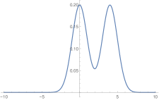
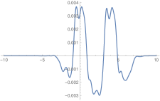
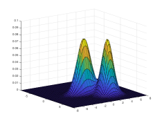
In order to illustrate our approach we provide a simple example with a bimodal distribution in dimension . Although this example is in one variable, it allows us to emphasize the differences between the existing KDE methods and our approach. We generate test data by using two normal distributions with means and . The exact PDF of this data is given by
| (4.3) |
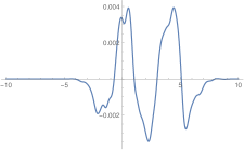
where . We then use KDE implemented in Mathematica with the Gaussian kernel . Using data samples drawn from (4.3) (so that the initial sum (4.1) has terms), the scaling parameter was set to . The true distribution (4.3) and the approximation error obtained by Mathematica by reducing (4.1) from terms to 241 Gaussian terms centered on an equally spaced grid are displayed in Figure 4.1. Using our algorithm with the same parameter , we reduce (4.1) from terms to 102 terms centered at a selected subset of the original data points. The error of the resulting approximation is displayed in Figure 4.1, where we also show the difference between (4.1) and (4.2). The main point here is that while the standard approach in high dimensions becomes impractical (as it requires a multidimensional grid), our approach proceeds unchanged since the cost of the reduction algorithm depend on dimension only mildly.
Remark 8.
We selected a much higher accuracy for reduction than the difference between the original and estimated PDFs in order to illustrate the fact that the accuracy limit of Algorithm 1 of about to digits is more than sufficient for this application. Note that to achieve a comparable accuracy for estimation of a PDF via KDE one needs points since the accuracy improves as .
Remark 9.
4.2. An example in high dimensions
We generate samples from a two dimensional Gaussian distribution with the PDF
where , , and
We pad these samples with zeros so that they belong to a -dimensional space and denote them by . We then apply a random rotation matrix to obtain the test data . As the bandwidth parameter, we set
a value that minimizes the mean integrated square error for an underlying standard normal distribution (see e.g. [42]). In our case, since the intrinsic dimension of the test data is , we set . The initial kernel density estimator using all test data is
| (4.4) |
where is the -by- identity matrix. We then reduce the number of terms in using Algorithm 1 and obtain a sum of Gaussians with fewer terms,
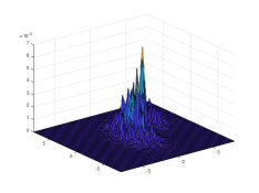
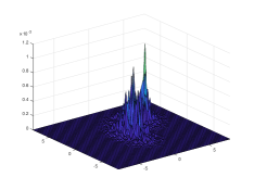
In our experiments, we choose dimensions and error threshold in Algorithm 1. The number of terms after reduction is about for all dimensions and the approximation error is about (see Figure 4.2).
In order to compare our approximation with the true PDF , we consider a point such that, under the rotation , we have . Evaluating (4.4) at , we obtain
where and denote the -th component of . Notice that the kernel density estimator for the PDF of the original distribution in two dimensions is
Therefore, to estimate the size of the approximation error, we generate a set of equispaced grid points , in . We pad each with zeros to embed it into , which we denote as . We then apply the same rotation matrix to obtain a set of points . In Figure 4.2 we illustrate the result for dimension ; we show the PDF , the errors between and the KDE estimate before reduction and the estimate after reduction, as well as the difference between and .

5. Far-field summation in high dimensions
Given a large set of points in dimension with pairwise interaction via a non-oscillatory kernel, our approach provides a deterministic algorithm for fast summation in the far-field setup (i.e. where two groups of points are separated). Recently a randomized algebraic approach in a similar setup was suggested in [35]. Instead, we use Algorithm 1 as a tool to rapidly evaluate
where and are large and is a non-oscillatory kernel with a possible singularity at (recall that kernels of mathematical physics typically have a singularity for coincident arguments and ).
Let us consider sources and targets occupying two distinct -dimensional balls. Specifically, we assume that and , where , and , are the centers and the radii of the balls. We also assume that sources and targets are separated, i.e., . The separation of sources and targets implies that in the evaluation of the kernel we are never close to a possible singularity of the kernel at . Separation of sources and targets allows us to use a non-singular approximation of the kernel and reduce the problem to finding the best linearly independent subsets of sources (or targets) as defined by such approximate kernel. We also assume that the sources are located on a low-dimensional manifold embedded in high-dimensional space (see Remark 12 below).
In order to use Algorithm 1, we need to define an inner product that takes into account the assumption of separation of sources and targets. We illustrate this using the example of the Poisson kernel (3.3), (without standard normalization). Approximating as in Section 3.1 (c.f. (3.4)), we have
| (5.1) |
Since sources and targets are separated,we drop terms in (5.1) with sufficiently large exponents (they produce a negligible contribution in the interval ) as well as replace terms with small exponents using an algorithm described in [12]. As a result, we obtain
such that
where is slightly larger than . It follows that
where
Since implies , we define the inner product as an integral over the ball ,
| (5.2) |
The inner product (5.2) can be reduced to a one dimensional integral, as we show next.
where
and
Using spherical coordinates in dimensions , we obtain
| (5.3) | |||||
where is the surface area of the -dimensional sphere embedded in -dimensional space, i.e., and is the -th order modified Bessel function of the first kind (see [1, Eq. 9.6.18]). While in odd dimensions the integrand in (5.3) can be extended from to as a smooth function allowing us to use the trapezoidal rule, such extension is not available in even dimensions. Because of this, we choose to use quadratures on developed in [10] (alternatively, one can use quadratures from [2]).
Remark 10.
It is an important observation that the selection of the inner product for finding a linearly independent subset of functions is not limited to the standard one defined in (5.2). Observing that (5.2) approaches zero as increases, in all of our experiments in dimensions , we use (5.2) where we set . Thus, the inner product no longer corresponds to the integral between the functions and . However, since we use inner products only to identify the best linearly independent subset of sources (skeleton sources) and compute the coefficients to replace the remaining terms as linear combinations of these skeleton sources, there are many choices of inner products that will produce similar results.
Associating with each the source function , we use Algorithm 1 to find the skeleton terms (i.e. the skeleton sources) with indices allowing us to express the remaining source functions (for ) as
Remark 11.
Using Algorithm 1 to find the skeleton sources requires operations and computing interactions between skeleton sources and targets requires additional operations. Clearly, instead of working with sources, we can work with targets. If targets are located on a low-dimensional manifold, we can associate the functions with targets and use Algorithm 1 to find the skeleton targets. In such case, the computational cost becomes , where is the number of skeleton targets.
Remark 12.
If sources are chosen from a random distribution in rather than located in a small neighborhood of a low-dimensional manifold, the expected distance between two sources becomes increasingly large as the dimension increases (see e.g. comments in [41, Section 1.5.3] and examples in [35]). As a result, the functions of variable , and , are effectively linearly independent as becomes large so that in order to have compressibility, the sources must have a low intrinsic dimension. Therefore, the assumption that sources are located in a small neighborhood of a low-dimensional manifold is not specific to our approach.
5.1. Skeleton sources
We illustrate our approach using sources located on a two-dimensional manifold embedded in a high-dimensional space. For our example, we generate points so that the first two coordinates are random variables drawn from the two-dimensional standard normal distribution and the remaining coordinates are set to zero. Next we apply a random rotation and rescale the points so that for all . For targets, we draw points from the -dimensional standard normal distribution and rescale them so that . We then shift the first component of by and that of by so that sources and targets are well separated. Finally, we select the coefficients of sources, , from the uniform distribution . In all tests we set and . In Table 7 we report the actual minimal and maximum distances between sources and targets ( and ), the number of skeleton sources , and the relative error of the approximation,
| (5.4) |
for selected dimensions . For dimensions , we use the Poisson kernel while for , we use the kernel (the fast decay of results in a negligible interaction between sources and targets in our setup).
5.2. Equivalent sources
In this example, we consider a similar setting as in Section 5.1 for We want to replace true sources located inside a ball by equivalent sources on its boundary as to reproduce their interaction with the targets within a selected accuracy . We expect the number of equivalent sources on the boundary to be significantly smaller than the number of original true sources so that pairwise interactions with targets can be computed rapidly. We note that such strategy is used in many numerical algorithms (see e.g. [48]) and here we demonstrate that our reduction algorithm can solve this problem.
We combine an initial set of candidate equivalent sources (note that their number will be reduced by the procedure) with the true sources and compute the Cholesky decomposition of their Gram matrix. We use Algorithm 1 with the inner product defined in (5.2) and modify the pivoting strategy to first pivot only among the candidate equivalent sources until we run out of significant pivots (i.e., pivots above the accuracy ); only then we switch to pivot among the true sources. Finally, we compute new coefficients in the usual way (see Algorithm 1) noting that, initially, the candidate equivalent sources had zero coefficients. This approach allows us to (i) obtain the minimal number of equivalent sources and (ii) remove as many of the true sources as possible (we do not preclude the possibility of some of the true sources to remain).
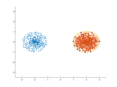
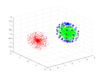
To examine the performance of our approach, we draw source and target points from the -dimensional standard normal distribution (where ), rescale and translate these points so that targets are located in a ball of radius centered at and sources are located in a ball of radius centered at . We choose , for and for to make sure sources and targets are well separated. Next we pick locations for the candidate equivalent sources on the surface of the ball of radius centered at . In dimension , we pick
where the angles are equally spaced on with step size . In dimension we pick
where the angles are equally spaced on with step size and the angles are the Gauss-Legendre nodes on . In our experiments we choose a relatively small number of true sources and targets () so that the result can be clearly visualized (see Figure 5.2 and 5.2). Note that the number of sources can be significantly higher since the algorithm is linear in this parameter. We demonstrate the results in Figure 5.2 and 5.2, where we display the original sources and targets and indicate both, candidate equivalent sources and selected equivalent sources obtained by Algorithm 1.
5.3. Partitioning of points into groups
Reduction Algorithm 1 can be used to subdivide scattered points into groups. Indeed, if a set of points (seeds) are specified beforehand then, like in Voronoi decomposition, all points can be split into groups by their proximity to the seeds, i.e. a point belongs to a group associated with a given seed if it is the closest to it among all seeds. There are several algorithms, e.g. Lloyd’s algorithm [33], that use such seeds in an iterative procedure to optimize some properties of the sought subdivision. The question then becomes how to choose such seeds. In order to avoid poor clusterings the so-called k-means++ algorithm is often used [3]. We would like to point out that Algorithm 1 can be used to generate initial seeds using linear dependence (which is a proxy for distances between points). We only illustrate its potential use for selecting seeds and provide no comparison with k-means++ or spectral clustering algorithms (see e.g. [38] and references therein). We also do not provide a comparison with model-based clustering (see e.g. [32, 37]). Using Algorithm 1 to subdivide scattered points into groups requires further analysis and we plan to address it elsewhere.
For our experiment, we use the same set of points as in Section 4.2 and associate with each point a Gaussian centered at that point. The scale parameter of the Gaussians can be selected sufficiently large (so that the Gaussian is sufficiently flat) to cover the whole set of points. We can then use Algorithm 1 to select the seeds. In order to force Algorithm 1 to select a specific first point, we introduce an additional point as the mean
and associate it with an additional Gaussian which we place at the beginning of the list of Gaussian atoms.
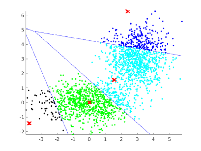
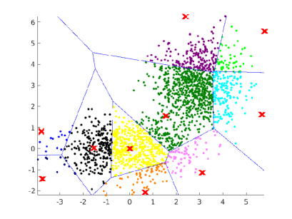
The seeds are the first significant pivots produced by the algorithm and our choice of their number depends on the goals of the subdivision. By its nature, Algorithm 1 tends to push these seeds far away from each other. We observe that groups with a small number of points appear to contain outliers (see Figure 5.3), so that the resulting subdivision can be helpful in identifying them. Since the computational cost of Algorithm 1 is , where is the original number of points and is the number of seeds, as long as the number of groups we are seeking is small, this algorithm is essentially linear. We note that we can subdivide the resulting groups further and, in a hierarchical fashion, build a tree structure. In this paper we simply illustrate the use of Algorithm 1 for subdivision of points into groups and plan to develop applications of this approach elsewhere.
For the example in Figure 5.3 we use the two dimensional distribution of points described in Section 4.2. We choose the bandwidth parameter when selecting 4 seeds and when selecting 10 seeds in order to obtain the corresponding subdivisions of the set. Observe that outliers tend to be associated with linearly independent terms and, thus, form a subset with a small number of points.
6. Conclusions and further work
We presented fast algorithms for reducing the number of terms in non-separated multivariate mixtures, analyzed them, and demonstrated their performance on a number of examples. These reduction algorithms allow us to work with non-separated multivariate mixtures which are a far reaching generalization of multivariate separated representations [8, 9, 7] and can be used as a tool for solving a variety of multidimensional problems. Further work is required to develop new numerical methods that use non-separated multivariate mixtures in applications, for example in quantum chemistry. We plan to pursue several multivariate problems with the techniques illustrated in this paper. Specifically, we plan to develop further our approach to KDE and compare it with existing techniques. We also plan to pursue the problem of hierarchical subdivision of point clouds into groups and its applications to clustering and detection of outliers.
Acknowledgements
We would like to thank Zydrunas Gimbutas (NIST) and the anonymous reviewers for their many useful comments and suggestions.
7. Appendix A
As mentioned in the paper, computing with multivariate Gaussian mixtures is particularly convenient since all common operations result in explicit integrals. We present below the key identities for multivariate Gaussians using the standard normalization,
However, when computing integrals with Gaussians atoms, it is convenient to normalize them to have unit -norm.
7.0.1. Convolution of two normal distributions
| (7.1) |
7.0.2. Sum of two quadratic forms
Consider vectors , , and and two symmetric positive definite matrices and . We have
where
and
7.0.3. Product of two normal distributions
We have
| (7.2) |
where
7.0.4. Inner product of two normal distributions
It follows that
References
- [1] Milton Abramowitz and Irene A. Stegun. Handbook of Mathematical Functions, volume 55 of Applied Math Series. National Bureau of Standards, 1964.
- [2] Bradley K. Alpert. Hybrid Gauss-trapezoidal quadrature rules. SIAM J. Sci. Comput., 20(5):1551–1584, 1999.
- [3] D. Arthur and S. Vassilvitskii. k-means++: The advantages of careful seeding. In Proceedings of the eighteenth annual ACM-SIAM symposium on Discrete algorithms, pages 1027–1035. Society for Industrial and Applied Mathematics, 2007.
- [4] A. Bernacchia and S. Pigolotti. Self-consistent method for density estimation. Journal of the Royal Statistical Society: Series B (Statistical Methodology), 73(3):407–422, 2011.
- [5] G. Beylkin, R. Coifman, and V. Rokhlin. Fast wavelet transforms and numerical algorithms, I. Comm. Pure Appl. Math., 44(2):141–183, 1991. Yale Univ. Technical Report YALEU/DCS/RR-696, August 1989.
- [6] G. Beylkin, G. Fann, R. J. Harrison, C. Kurcz, and L. Monzón. Multiresolution representation of operators with boundary conditions on simple domains. Appl. Comput. Harmon. Anal., 33:109–139, 2012. http://dx.doi.org/10.1016/j.acha.2011.10.001.
- [7] G. Beylkin, J. Garcke, and M. J. Mohlenkamp. Multivariate regression and machine learning with sums of separable functions. SIAM Journal on Scientific Computing, 31(3):1840–1857, 2009.
- [8] G. Beylkin and M. J. Mohlenkamp. Numerical operator calculus in higher dimensions. Proc. Natl. Acad. Sci. USA, 99(16):10246–10251, August 2002.
- [9] G. Beylkin and M. J. Mohlenkamp. Algorithms for numerical analysis in high dimensions. SIAM J. Sci. Comput., 26(6):2133–2159, July 2005.
- [10] G. Beylkin and L. Monzón. On generalized Gaussian quadratures for exponentials and their applications. Appl. Comput. Harmon. Anal., 12(3):332–373, 2002.
- [11] G. Beylkin and L. Monzón. On approximation of functions by exponential sums. Appl. Comput. Harmon. Anal., 19(1):17–48, 2005.
- [12] G. Beylkin and L. Monzón. Approximation of functions by exponential sums revisited. Appl. Comput. Harmon. Anal., 28(2):131–149, 2010.
- [13] G. Beylkin, L. Monzón, and I. Satkauskas. On computing distributions of products of random variables via Gaussian multiresolution analysis. Appl. Comput. Harmon. Anal., 2017. doi: 10.1016/j.acha.2017.08.008, see also arXiv:1611.08580.
- [14] D. J. Biagioni, D. Beylkin, and G. Beylkin. Randomized interpolative decomposition of separated representations. Journal of Computational Physics, 281:116–134, 2015.
- [15] Åke Björck. Solving linear least squares problems by gram-schmidt orthogonalization. BIT Numerical Mathematics, 7(1):1–21, 1967.
- [16] Z. I. Botev, J. F. Grotowski, and D. P. Kroese. Kernel density estimation via diffusion. The Annals of Statistics, 38(5):2916–2957, 2010.
- [17] S. F. Boys. The integral formulae for the variational solution of the molecular many-electron wave equations in terms of gaussian functions with direct electronic correlation. Proceedings of the Royal Society of London Series A- Mathematical and Physical Sciences, 258(1294):402, 1960.
- [18] R. Bro. Parafac. Tutorial and Applications. Chemometrics and Intelligent Laboratory Systems, 38(2):149–171, 1997.
- [19] J. D. Carroll and J. J. Chang. Analysis of individual differences in multidimensional scaling via an N-way generalization of Eckart-Young decomposition. Psychometrika, 35:283–320, 1970.
- [20] G. C. Cawley and N. L. C. Talbot. Reduced rank kernel ridge regression. Neural Processing Letters, 16(3):293–302, 2002.
- [21] S. Chandrasekaran and I. C. F Ipsen. On rank-revealing factorisations. SIAM Journal on Matrix Analysis and Applications, 15(2):592–622, 1994.
- [22] Bengt Fornberg and Natasha Flyer. A primer on radial basis functions with applications to the geosciences. SIAM, 2015.
- [23] L. Genovese, T. Deutsch, A. Neelov, S. Goedecker, and G. Beylkin. Efficient solution of Poisson’s equation with free boundary conditions. J. Chem. Phys., 125(7), 2006.
- [24] G. Golub and C. Van Loan. Matrix Computations. Johns Hopkins University Press, 3rd edition, 1996.
- [25] M. Gu and S. C. Eisenstat. Efficient algorithms for computing a strong rank-revealing qr factorization. SIAM Journal on Scientific Computing, 17(4):848–869, 1996.
- [26] N. Halko, P.-G. Martinsson, and J. A. Tropp. Finding structure with randomness: probabilistic algorithms for constructing approximate matrix decompositions. SIAM Review, 53(2):217–288, 2011.
- [27] R. J. Harrison, G. Beylkin, F. A. Bischoff, J. A. Calvin, G. I. Fann, J. Fosso-Tande, D. Galindo, J.R Hammond, R. Hartman-Baker, J. C Hill, et al. Madness: A multiresolution, adaptive numerical environment for scientific simulation. SIAM J. Sci. Comput., 38(5):S123–S142, 2016. see also arXiv preprint arXiv:1507.01888.
- [28] R.J. Harrison, G.I. Fann, T. Yanai, Z. Gan, and G. Beylkin. Multiresolution quantum chemistry: basic theory and initial applications. J. Chem. Phys., 121(23):11587–11598, 2004.
- [29] R. A. Harshman. Foundations of the Parafac procedure: model and conditions for an “explanatory” multi-mode factor analysis. Working Papers in Phonetics 16, UCLA, 1970.
- [30] R. A. Horn and C. R. Johnson. Matrix analysis. Cambridge University Press, Cambridge, second edition, 2013.
- [31] T. G. Kolda and B. W. Bader. Tensor decompositions and applications. SIAM Review, 51(3):455–500, 2009.
- [32] J. Li, S. Ray, and B. G. Lindsay. A nonparametric statistical approach to clustering via mode identification. Journal of Machine Learning Research, 8(Aug):1687–1723, 2007.
- [33] S. Lloyd. Least squares quantization in pcm. IEEE transactions on information theory, 28(2):129–137, 1982.
- [34] J.V.L. Longstaff and K. Singer. The use of gaussian (exponential quadratic) wave functions in molecular problems. ii. wave functions for the ground state of the hydrogen atom and of hydrogen molecule. Proc. R. Soc. London Ser. A-Math., 258(1294):421, 1960.
- [35] W. B. March and G. Biros. Far-field compression for fast kernel summation methods in high dimensions. Applied and Computational Harmonic Analysis, 43(1):39–75, 2017.
- [36] V. Maz’ya and G. Schmidt. Approximate approximations, volume 141 of Mathematical Surveys and Monographs. American Mathematical Society, Providence, RI, 2007.
- [37] P. D. McNicholas. Model-based clustering. Journal of Classification, 33(3):331–373, 2016.
- [38] A. Y. Ng, M. I. Jordan, and Y. Weiss. On spectral clustering: Analysis and an algorithm. In Advances in neural information processing systems, pages 849–856, 2002.
- [39] T. A. O’Brien, K. Kashinath, N. R Cavanaugh, W. D Collins, and J. P O’Brien. A fast and objective multidimensional kernel density estimation method: fastkde. Computational Statistics & Data Analysis, 101:148–160, 2016.
- [40] M. Reynolds, A. Doostan, and G. Beylkin. Randomized alternating least squares for canonical tensor decompositions: application to a PDE with random data. SIAM J. Sci. Comput., pages A2634–A2664, 2016.
- [41] D. W. Scott. Multivariate density estimation: theory, practice, and visualization. John Wiley & Sons, 2015.
- [42] B. W. Silverman. Density estimation for statistics and data analysis, volume 26. CRC press, 1986.
- [43] K. Singer. The use of gaussian (exponential quadratic) wave functions in molecular problems. i. General formulae for the evaluation of integrals. Proc. R. Soc. London Ser. A-Math., 258(1294):412, 1960.
- [44] G. Tomasi and R. Bro. A comparison of algorithms for fitting the PARAFAC model. Comput. Statist. Data Anal., 50(7):1700–1734, 2006.
- [45] F. Vico, L. Greengard, and M. Ferrando. Fast convolution with free-space green’s functions. Journal of Computational Physics, 323:191–203, 2016.
- [46] T. Yanai, G.I. Fann, Z. Gan, R.J. Harrison, and G. Beylkin. Multiresolution quantum chemistry: Analytic derivatives for Hartree-Fock and density functional theory. J. Chem. Phys., 121(7):2866–2876, 2004.
- [47] T. Yanai, G.I. Fann, Z. Gan, R.J. Harrison, and G. Beylkin. Multiresolution quantum chemistry: Hartree-Fock exchange. J. Chem. Phys., 121(14):6680–6688, 2004.
- [48] L. Ying, G. Biros, and D. Zorin. A kernel-independent adaptive fast multipole algorithm in two and three dimensions. Journal of Computational Physics, 196(2):591–626, 2004.