Multiphase Partitions of Lattice Random Walks

Abstract

Considering the dynamics of non-interacting particles randomly moving on a lattice, the occurrence of a discontinuous transition in the values of the lattice parameters (lattice spacing and hopping times) determines the uprisal of two lattice phases. In this Letter we show that the hyperbolic hydrodynamic model obtained by enforcing the boundedness of lattice velocities derived in [20] correctly describes the dynamics of the system and permits to derive easily the boundary condition at the interface, which, contrarily to the common belief, involves the lattice velocities in the two phases and not the phase diffusivities. The dispersion properties of independent particles moving on an infinite lattice composed by the periodic repetition of a multiphase unit cell are investigated. It is shown that the hyperbolic transport theory correctly predicts the effective diffusion coefficient over all the range of parameter values, while the corresponding continuous parabolic models deriving from Langevin equations for particle motion fail. The failure of parabolic transport models is shown via a simple numerical experiment.

Lattice models of particle dynamics represent a robust conceptual backbone in statistical theory of non-equilibrium processes, finding broad and diversified applications in practically all the branches of physics [1, 2]. They constitute a simple gedanke experimental enviroment in order to derive, from simple local interaction rules, the corresponding hydrodynamic models in a continuous space-time setting [3, 4].

Even in the case of systems of noninteracting particles, a rich variety of possible phenomenologies arises, associated with lattice heterogeneities and impurities [5], randomly distributed multisite structures [6, 7], disorder, percolation and phase transitions [8], anomalous behavior induced by a continuous distribution of hopping times and hopping lengths (that can be treated within the framework of Continuous Time Random Walk) [9, 10], etc.

In recent years, lattice heterogeneity has been studied in connection with infiltration dynamics, and solute partition in two lattice phases, defined by the decomposition of the lattice in two subsets possessing different lattice parameters [11, 12, 13, 14, 15]. The latter problem has great current interest in biological applications involving active swimmers moving in nonuniform fields modulating their mobilities [16], and is connected to fundamental problems involving the stochastic modeling of non-equilibrium phenomena, associated with the proper choice of the most suitable stochastic calculus (Ito, Stratonovich, Hänggi-Klimontovich) [17, 18], and with the properties of the equilibrium invariant densities and their connection with local transport properties [19].

Although the current research focus is mostly oriented towards particle motion determining the occurrence of anomalous diffusive phenomena [12], the case of the simplest possible model of lattice random walk involving noninteracting particles has shown that some interesting properties are still to be unveiled, especially as regards its continuous hydrodynamic description. It has been shown recently in [20] that the the classical lattice random walk of independent particles can be described in a continuous space-time setting by means of a hyperbolic transport model analogous to those arising in the theory of Generalized Poisson-Kac processes [21, 22]. The hyperbolic transport model accounts intrinsically for the finite propagation velocity of the process, and provides an accurate quantitative description not only of the long-term properties but also of the initial stages of the dynamics [20]. In the case of a symmetric lattice random walk, defined by the characteristic site distance $\delta$ and hopping time $\tau$ between nearest neighboring sites, the hyperbolic continuous model involves the partial probabilities $\{p_{\pm}(x,t)\}$, where $p_{\pm}(x,t)\,dx$ is the fraction of particles in the spatial interval $(x,x+dx)$ at time $t$ moving towards the right ($p_{+}$) or to the left ($p_{-}$), satisfying the equations

$$\frac{\partial p_{\pm}(x,t)}{\partial t}=\mp b\,\frac{\partial p_{\pm}(x,t)}{\partial x}\mp\lambda\,\left[p_{+}(x,t)-p_{-}(x,t)\right]$$ (1)

where $b=\delta/\tau$, and $\lambda=1/\tau$ (see the Appendix). The overall probability density of the process is $p(x,t)=p_{+}(x,t)+p_{-}(x,t)$, and the associated flux $J(x,t)=b\,[p_{+}(x,t)-p_{-}(x,t)]$.

In this work, we consider the multiphase extension of the symmetric random walk, as depicted in figure 1. The MultiPhase Lattice Random Walk, henceforth MuPh-LRW for short, is a simple random walk on a lattice ${\mathbb{Z}}$, in which the physical lattice parameters $(\delta,\tau)$ admit a sudden transition at some lattice point, say $z_{0}\in{\mathbb{Z}}$ so that $(\delta_{1},\tau_{1})$ holds for $z<z_{0}$, and $(\delta_{2},\tau_{2})$ for $z>z_{0}$. The lattice point $z_{0}$ represents the interfase separating the two lattice phases.

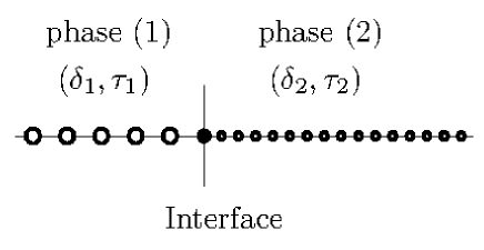
Figure 1: Schematic representation of a MuPh-LRW.

Within each lattice phase particle motion is a symmetric LRW, corresponding, in the continuous limit, to an emergent purely diffusive behavior defined by the phase diffusivities $D_{h}=\delta_{h}^{2}/2\tau_{h}$, $h=1,2$. It remains to specify the motion at the interfacial point $z_{0}$. Two cases can occur: (i) if the interfacial point is “neutral” with respect to phase selection, so that equal probabilities characterize the jump from $z_{0}$ to one of its two nearest neighboring sites, the interface is referred to as ideal; (ii) if the probabilities of moving from the interface towards the sites of one of the two phases are different, the interface exerts a specific and active selection, and it will be referred to as non ideal or active. In this Letter we focus exclusively on ideal interfaces.

In a discrete space-time description, the MuPh-LRW corresponds to a simple symmetric LRW defined by the dynamics $z_{n+1}=z_{n}\pm 1\;\mbox{Prob}.\;1/2$, where $n=0,1,\dots$ is the lattice time. In a physical setting, indicating with $x_{n}$ the particle spatial position and $t_{n}$ the physical time, MuPh-LRW corresponds to a subordination of the stochastic lattice motion according to phase heterogeneity. More precisely, let $\sigma_{n}=\sigma(x_{n})$ be the phase-function, $\sigma_{n}=\{1,2,0\}$, depending whether the site $x_{n}$ belongs to phase “1”, “2”, or is an interfacial site (“0”)., the MuPh-LRW dynamics in the presence of ideal interfaces is defined by

$$x_{n+1} = x_{n}+\mbox{sgn}(x_{n+1}-x_{n})\,M[\sigma_{n},\sigma_{n\pm 1}]\;\;\;\mbox{Prob}.\;1/2$$

$$t_{n+1} = t_{n}+T[\sigma_{n},\sigma_{n+1}]$$ (2)

where $\mbox{sgn}(\cdot)$ is the sign function, and in which the symmetric matrices $M[s_{1},s_{2}]$, $T[s_{1},s_{2}]$ are defined by the transport (metric and temporal) properties of the two phases, $M[h,h]=M[0,h]=M[h,0]=\delta_{h}$, $T[h,h]=T[0,h]=T[h,0]=\tau_{h}$, $h=1,2$.

Two main questions arise: (i) the definition of a continuous hydrodynamic model for MuPh-LRW, and (ii), strictly connected to (i), the assessment of the proper boundary condition at an ideal interface in a continuous setting of the dynamics. These two issues are closely related to each other. As regards the hydrodynamic description, the hyperbolic approach introduced in [20] can be applied to each phase. This corresponds to consider eq. (1) for each phase, with $p_{\pm}(x,t)$ substituted by the phase partial concentration $p_{\pm}^{(h)}(x,t)$, defined for $x$ within each disjoint domain of definition of the phases, and $b$ and $\lambda$ with $b_{h}=\delta_{h}/\tau_{h}$, $\lambda_{h}=1/\tau_{h}$. This follows also from eq. (2) by considering the subordination of the physical time $t$ with respect to the lattice time $n$ for processes possessing finite propagation velocity (Poisson-Kac processes) (see the Appendix). In the case of ideal interfaces, there is no active effect of the interface on the partition of solute particles in the two phases, and the hyperbolic approach based on eq. (1) implies the continuity of the partial fluxes across an ideal interface located at $x_{0}$ (corresponding to the lattice coordinate $z_{0}$),

$$\left.b_{1}\,p_{\pm}^{(1)}(x,t)\right|_{x=x_{0}}=\left.b_{2}\,p_{\pm}^{(2)}(x,t)\right|_{x=x_{0}}$$ (3)

This condition can be further justified by enforcing the lattice representation of the dynamics, consistently with the analysis developed in the Appendix. Eq. (3) obviously predicts the continuity of the normal fluxes at the interface, $J^{(1)}(x_{0},t)=J^{(2)}(x_{0},t)$, and the boundary condition for the overall particle density

$$\left.\frac{p^{(2)}(x,t)}{p^{(1)}(x,t)}\right|_{x=x_{0}}=\frac{b_{1}}{b_{2}}=\frac{\delta_{1}\,\tau_{2}}{\delta_{2}\,\tau_{1}}$$ (4)

In point of fact, eq. (4) represents a change of paradigm with respect to the usual approach to boundary conditions applied at interfaces in the presence of diffusion, in which $p^{(2)}/p^{(1)}|_{x=x_{0}}$ is assumed equal to the ratio of the diffusivities $D_{1}/D_{2}$ [11, 13, 14, 15]. Eq. (3) finds its natural explanation in the stochastic models in which the finite value of the propagation velocities $b_{h}$ is assumed, while it is “alien” to the classical parabolic approach. In this framework, the analysis of MuPh-LRW is a significant benchmark to test the importance of the physical assumptions underlying hyperbolic transport theories [22, 24, 25].

Direct numerical simulations of MuPh-LRW provides a clear answer to this question. Consider a MuPh-LRW on a closed domain $x\in[-1,1]$ equipped with zero-flux conditions at the endpoints. The interval $[-1,0)$ corresponds to the lattice phase “1”, $(0,1]$ to the lattice phase “2”, and the interface is located at $x=x_{0}=0$. In the simulations, $\delta_{1}=1/N$, $N_{1}=N$ is the number of lattice sites in phase “1”, $\delta_{2}=\delta_{1}/\alpha$, where $\alpha$ is an integer, so that $N_{2}=\alpha\,N$ is the number of sites of phase “2”, while $\tau_{1}=1$ and $\tau_{2}$ freely varies. An ensemble of $10^{6}$ particles is considered, initially located at the interface.

Figures 2 and 3 depict the comparison of the lattice simulations of MuPh-LRW with the results obtained by integrating the hyperbolic equations (1) for each phase and in each disjoint phase domain where the boundary conditions 3 have been applied at the interface $x=0$. Figure 2 refers to $\delta_{2}=\delta_{1}/4$, $\tau_{2}=\tau_{1}$, so that $p^{(2)}/p^{(1)}|_{x=0}=4$, while the classical diffusive boundary condition provides $p^{(2)}/p^{(1)}=16$. Figure 3 refers to $\delta_{2}=\delta_{1}/2$, $\tau_{2}=\tau_{1}/2$, at which the hyperbolic theory predicts a smooth overall concentration profile across the interface as $p^{(2)}/p^{(1)}|_{x=0}=1$, while the diffusive boundary condition implies a discontinuity $p^{(2)}/p^{(1)}|_{x=0}=2$.

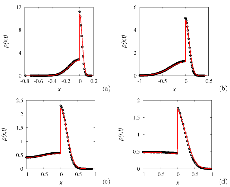
Figure 2: Probability density function $p(x,t)$ vs $x$ at several time instants for $\delta_{2}=\delta_{1}/4$, $\tau_{2}=\tau_{1}$. Symbols ($\circ$) are the results of lattice simulations, continuous lines the solutions of the corresponding hyperbolic model. Panel (a) refers to $t=2\times 10^{2}$, (b) to $t=10^{3}$, (c) to $t=5\times 10^{3}$, (d) to $t=10^{4}$.

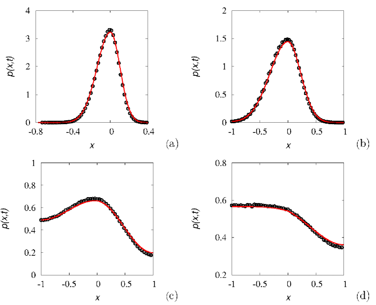
Figure 3: Same as in figure 2 at $\delta_{2}=\delta_{1}/2$, $\tau_{2}=1/2$.

The lattice simulation results are accurately described by the hyperbolic hydrodynamic model, and the validity of the velocity-based interfacial condition (4), or eq. (3), is highlighted by the data depicted in figure 4 referred to the particle fraction $p_{1}^{*}$ at steady state in phase “1”, obtained from lattice simulations, as a function of the ratio $\tau_{1}/\tau_{2}$, compared with the result deriving from eq. (4) and constrasted with the parabolic interpretation of the boundary conditions based on the ratio of the phase diffusivities.

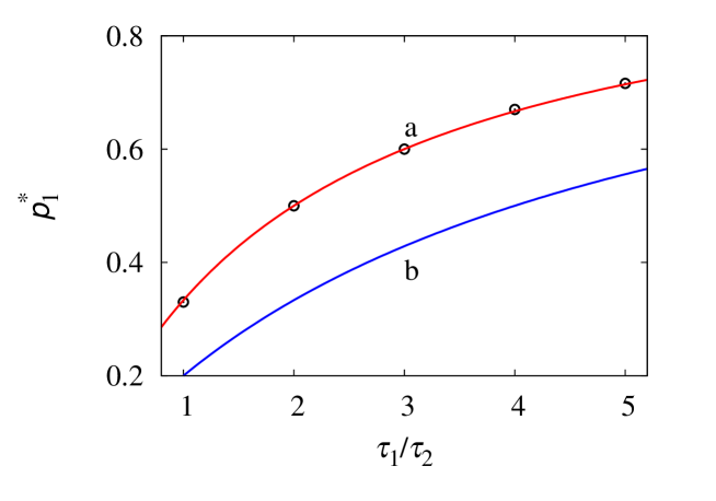
Figure 4: Particle frequency $p_{1}^{*}$ in phase “1” at steady state as a function of $\tau_{1}/\tau_{2}$ in a MuPh-LRW closed cell $x\in[-1,1]$ at $\delta_{2}=\delta_{1}/2$. Symbols are the results of lattice simulations, curve (a) corresponds to $p_{1}^{*}=(b_{2}/b_{1})\,p_{2}^{*}$, curve (b) to $p_{1}^{*}=(D_{2}/D_{1})\,p_{2}^{*}$.

Once the qualitative and quantitative validity of the hyperbolic description and of the interfacial conditions arising from it has been assessed, it is possible to use this hydrodynamic model to investigate finer transport properties of MuPh-LRW. Specifically, we consider a dispersion experiment on a lattice composed by the periodic repetition of a multiphase unit cell as depicted in figure 5.

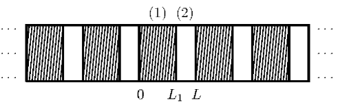
Figure 5: Schematic representation of a LRW in a periodic lattice structure possessing a multiphase unit periodicity cell.

The unit lattice structure is the same used for the data in figures 2 and 3, with physical length $L=2$, $L_{1}=L_{2}=1$ and $\delta_{1}=1/N$, where $N=N_{1}=100$, $\tau_{1}=1$, $\delta_{2}=\delta_{1}/\alpha$ and $\tau_{2}$ varies. By considering an ensemble of $10^{6}$ particles initially located at $z_{0}=0$ ($x_{0}=0$), the first order moments (mean and mean square displacement) are estimated, and from their linear scalings with time $t$ in the long-term regime, the value of the effective velocity $V_{\rm eff}$ and effective diffusivity $D_{\rm eff}$ (dispersion coefficient) obtained. From the simulations one obtains $V_{\rm eff}=0$, while the results for $D_{\rm eff}$ as a function of $\tau_{1}/\tau_{2}$, varying $\delta_{1}/\delta_{2}$ are depicted in figure 6.

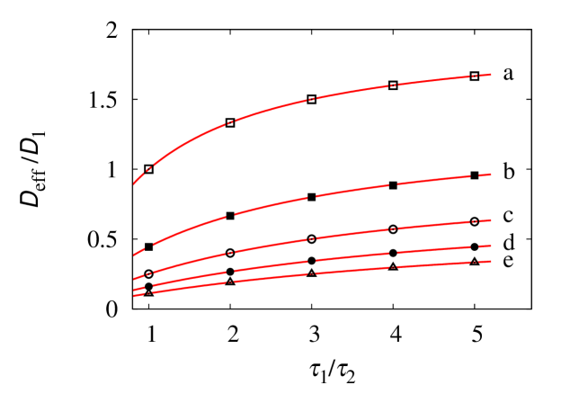
Figure 6: Dispersion coefficient $D_{\rm eff}/D_{1}$ for particle transport in a periodic multiphase lattice as a function of $\tau_{1}/\tau_{2}$. Symbols are the results of lattice simulations, solid lines the predictions of homogenization theory applied to the hyperbolic transport model. Line (a) and ($\square$) refers to $\delta_{1}/\delta_{2}=1$, line (b) and ($\blacksquare$) to $\delta_{1}/\delta_{2}=2$, line (c) and ($\circ$) to $\delta_{1}/\delta_{2}=3$, line (c) and ($\bullet$) to $\delta_{1}/\delta_{2}=4$, line (e) and ($\triangle$) to $\delta_{1}/\delta_{2}=5$.

These data should be compared with the long-term properties derived from the continuous hyperbolic model based on eq. (1) obtained from exact moment analysis [26]. In order to have a qualitative picture of the influence of the finite velocity assumption in the long-term hydrodynamic behavior of MuPh-LRW, we consider also the modeling of particle motion in terms of a Langevin equation driven by a Wiener process, and leading to a parabolic Fokker-Planck equation. Taking into account the nonlinear and discontinuous nature of the resulting Langevin equation, we consider the most general interpretation of it, namely $dx(t)=\sqrt{2\,D(x(t))}*_{\lambda}dw(t)$, where $D(x)=D(x+L)$ is the discontinuous and spatially periodic diffusivity profile attaining the values $D_{h}$ in each lattice phase, $dw(t)$ the increment of a Wiener process in the time interval $dt$ and “$*_{\lambda}$” indicates that the $\lambda$-calculus, $\lambda\in[0,1]$, has been chosen in the definition of the stochastic Stieltjes integrals ($\lambda=0,\,1/2,\,1$ correspond to the Ito, Stratonovich and Hänggi-Klimontovich interpretation, respectively) [27]. A detailed account of the exact homogenization analysis of the different hydrodynamic models can be found in [26]. The final result (for $L_{1}=L_{2}=1$) is

$$\frac{1}{D_{\rm eff}}=\frac{1}{2}\left(\frac{1}{b_{1}}+\frac{1}{b_{2}}\right)\left(\frac{1}{b_{1}\,\tau_{1}}+\frac{1}{b_{2}\,\tau_{2}}\right)$$ (5)

for the hyperbolic model, and

$$\frac{1}{D_{\rm eff}}=\frac{1}{4}\left(\frac{1}{D_{1}^{1-\lambda}}+\ \frac{1}{D_{2}^{1-\lambda}}\right)\left(\frac{1}{D_{1}^{\lambda}}+\ \frac{1}{D_{2}^{\lambda}}\right)$$ (6)

for the Langevin-Wiener model associated with a $\lambda$-interpretation of the stochastic integrals. The data depicted in figure 6 clearly indicate that the hyperbolic transport model accurately accounts for the dispersion properties in a multiphase lattice. Conversely, even keeping $\lambda$ as an adjustable parameter, it is impossible for any Langevin-Wiener model of MuPh-LRW diffusion to provide a quantitative estimate of the long-term dispersion properties. This claim is supported by the data depicted in figure 7. These data refer to the effective diffusion coefficient in a periodic multiphase lattice at $\delta_{2}=\delta_{1}/\gamma\,\xi$, $\tau_{2}=\tau_{1}/\xi^{2}$ by varying the parameters $\gamma$, and $\xi$. For fixed values of $\gamma$, the ratio $D_{1}/D_{2}=\gamma$ is constant. From eq. (6) it follows that any Langevin-Wiener model of particle transport would predict a constant value of $D_{\rm eff}$ independently of the value of $\xi$. Conversely, the hyperbolic model based on eq. (1) predicts a value of $D_{\rm eff}/D_{1}$ that depends continuously on the ratio $\tau_{1}/\tau_{2}=\xi^{2}$ for fixed $\gamma$. Lattice simulation results depicted in figure 7 support the latter prediction of the hyperbolic hydrodynamic model. In the case $D_{1}/D_{2}=1$, one has $D_{\rm eff}/D_{1}=1$ from the parabolic model, independently of $\lambda$ (line (c) in figure 7), while in general $D_{\rm eff}/D_{1}$in parabolic Langevin-Wiener models is lower- and upper-bounded by the values attained at $\lambda=0$ and $\lambda=1/2$ (see the Appendix).

This result indicates that the hyperbolic hydrodynamic model not only provides a more quantitatively consistent alternative to parabolic models for describing LRW at short timescales, as addressed in [20], but it is the only continuous model deriving from a continuous stochastic description of particle transport constistent with long-term dispersion data in multiphase periodic lattices.

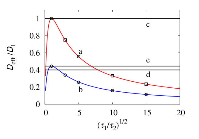
Figure 7: $D_{\rm eff}/D_{1}$ vs $(\tau_{1}/\tau_{2})^{1/2}$ for dispersion in a periodic multiphase lattice for a fixed ratio $D_{1}/D_{2}$. Symbols are the results of lattice simulations, solid lines (a) and (b) the predictions of the hyperbolic transport model eq. (5). Line (a) and ($\square$) refer to $D_{1}/D_{2}=1$, line (b) and ($\circ$) to $D_{1}/D_{2}=4$. The horizontal lines represent the lower and upper bounds in the predictions of the parabolic transport model obtained by varying $\lambda$: line (c) refers to $D_{1}/D_{2}=1$, line (d) and (e) to $D_{1}/D_{2}=4$.

Reversing the latter argument, it implies that the assumption of finite-time propagation velocity is a fundamental prerequisite in order to predict correctly both the long-time dispersion properties in infinite multiphase lattices and the equilibrium properties in closed multiphase cells.

The latter observation opens up interesting perspectives in the hydrodynamic modeling of particle systems based on the fundamental assumption of finite propagation velocity. This observation finds a significant experimental confirmation in the ubiquitous evidence of ballistic transport at short timescales both in micro- and nanostructures [28, 29, 30], and sheds new light on the conceptual relevance in non-equilibrium statistical physics of stochastic approaches deeply grounded on the “weak relativistic principle” of finite propagation velocity. The same approach can be extended to electron-transport in periodic lattices, in order to determine the effective electron mass in all the solid-state systems in which experimental evidence suggests an effective relativistic constraint associated with a bounded velocity of carrier particles [31, 32].

Appendix

These notes address some auxiliary observations and explanations complementing the results developed in the main text.

LRW and Hyperbolic Hydrodynamic Models

In [20] an hyperbolic hydrodynamic model for the classical asymmetric Lattice Random Walk (LRW) has been derived. Three parameters characterize a LRW: (i) $\delta$ the distance between nearest neighboring sites, (ii) $\tau$ the hopping time, and (iii) $r=r_{1}-r_{2}$ the difference between the probabilities of moving to the right ($r_{1}$) and the left ($r_{2}$), where $r_{1},\,r_{2}>0$, $r_{1}+r_{2}=1$. In the symmetric case, $r=0$, the hyperbolic model for the partial probability waves $p_{\pm}(x,t)$ reads

$$\frac{\partial p_{+}(x,t)}{\partial t} = -b\,\frac{\partial p_{+}(x,t)}{\partial x}-\lambda\,\left[p_{+}(x,t)-p_{-}(x,t)\right]$$

$$\frac{\partial p_{-}(x,t)}{\partial t} = b\,\frac{\partial p_{-}(x,t)}{\partial x}+\lambda\,\left[p_{+}(x,t)-p_{-}(x,t)\right]$$ (7)

where $b=\delta/\tau$ is the finite lattice velocity. Regarding the relation between $\lambda$ and $\tau$ in the symmetric case, it is important to observe the following. The statistical description defined by eq. (7) can be interpreted in the symmetric case in two ways, in the meaning that two different Generalized Poisson-Kac (GPK) processes [22] give rise to the same statistical description.

A GPK process possessing $N=2$ stochastic states on the real line ${\mathbb{R}}$, is defined by a system of velocities $b_{1}=b$, $b_{2}=-b$, referred to the two stochastic states, a vector of transition rates $\boldsymbol{\Lambda}=(\lambda_{1},\lambda_{2})$ and a transition probability matrix ${\bf A}=(A_{\alpha,\beta})_{\alpha,\beta=1}^{2}$ [22]. The latter two quantities define the 2-state finite Poisson process $\chi_{2}(t;{\boldsymbol{\Lambda}},{\bf A})$ that is essentially a 2-state Markov chain, so that the dynamics is specified by the stochastic differential equation

$$dx(t)=b_{\chi_{2}(t;{\boldsymbol{\Lambda}},{\bf A})}\,dt$$ (8)

In the application of GPK models to LRW, the transitions rates are equal, i.e., $\lambda_{1}=\lambda_{2}=\lambda$.

The first GPK model corresponds to the choice $\lambda=2/\tau$ and

$${\bf A}=\frac{1}{2}\,\left(\begin{array}[]{ll}1&1\\ 1&1\end{array}\right)$$ (9)

which corresponds to the assumption of equal probabilities of selecting one of the two stochastic states at any transition point. Observe that the definition of “stochastic state” adopted here for a GPK process has nothing to share with the concept of a lattice phase introduced in the main article for MuPh-LRW. The above GPK model corresponds to the approach followed in [20]. The second alternative is to choose

$$\lambda=\frac{1}{\tau}$$ (10)

defining the transition probability matrix as

$${\bf A}=\left(\begin{array}[]{ll}0&1\\ 1&0\end{array}\right)$$ (11)

in which at any transition point there is a switching to the other stochastic state (implying a reversal of velocity direction). This is the approach followed in the main text. In the latter case, eq. (8) reduces to the classical Poisson-Kac model

$$dx(t)=b\,(-1)^{\chi(t;\lambda)}\,dt$$ (12)

where $\chi(t;\lambda)$ is a classical Poisson process possessing transition rate $\lambda$.

Computational issues

In the simulations of a lattice multiphase unit cell reported in the main text we have chosen $\delta_{1}=1/N$ with $N=100$, $\tau_{1}=1$, letting $\delta_{2}$ and $\tau_{2}$ vary. Specifically, $\delta_{2}=\delta_{1}/\alpha$ where $\alpha=1,2,\dots$ is an integer. Since the multiphase cell has been defined in the interval $x\in[-1,1]$, this corresponds to consider $N_{1}=N$ sites for the lattice phase “1”, defined for $x\in[-1,0)$ and $N_{2}=\alpha\,N$ sites for phase “2” defined for $x\in(0,1]$.

The results obtained from stochastic lattice simulations of MuPh-LRW are not influenced by a finer representation of the lattice obtained by increasing $N$, if the timescale $\tau_{1}$ is properly rescaled. The most critical issue is related to the short-time behavior. Figure 8 depicts the comparison of two lattice experiments on a closed MuPh-LRW cell for two values of $N=100,\,300$. In the latter case, the value of $\tau_{1}$ as been rescaled to $\tau_{1}=1/9$.

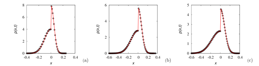
Figure 8: $p(x,t)$ vs $x$ for a MuPh-LRW in a closed cell $x\in[-1,1]$ at $\delta_{2}/\delta_{1}=1/2$, $\tau_{2}=\tau_{1}$ starting from an impulsive initial condition centered at the interfacial point. Symbols ($\bullet$) refer to simulations with $N=100$, $\tau_{1}=1$, lines to $N=300$, $\tau_{1}=1/9$. Panel (a) to (c) correspond to $t=100,\,200,\,300$, respectively.

There are no significant differences in the two simulations other than that the case $N=300$ obviously provides density profiles there are slightly more smooth.

A further comment refers to the initial conditions in a closed multiphase cell. We assumed that the initial condition is centered at the interface. In order to avoid unpleasent parity-effects associated with lattice random walk (if the initial condition is at an even site, then the concentration evaluated at even lattice times is vanishing at all the odd sites, and viceversa), the initial conditions has been distributed equally at site $z_{0}=0$ and at the first neighboring site belonging to phase “2”, i.e., $z_{1}=1$. In the solution of the continuous hyperbolic model this has been taken into account by considering an initial condition uniformly distributed within the interval $x\in[0,\delta_{2}]$. Moreover, in the simulations of the hyperbolic continuous model it has been assumed an initial balancing of the two partial probability waves, namely $p_{+}(x,0)=p_{-}(x,0)$.

The lattice simulation data reported in the main text refer to the long-term behavior of a closed MuPh-LRW system, once the dynamics has relaxed towards the equilibrium distribution $p^{*}(x)$. Figure 9 depicts the simulations results obtained for $p^{*}(x)$. Since the number of lattice particles considered is $N_{p}=10^{6}$, in order to obtain a statistically accurate estimate of the equilibrium distributions, reducing the fluctuations associated with finite-size effects in the particle ensemble, the stationary concentration profiles have been averaged over $N_{t}=10^{4}$ time instants, after reaching equilibrium conditions. The results of this averaging is depicted in figure 9 for $\delta_{2}=\delta_{1}/2$ at three different values of $\tau_{2}/\tau_{1}$.

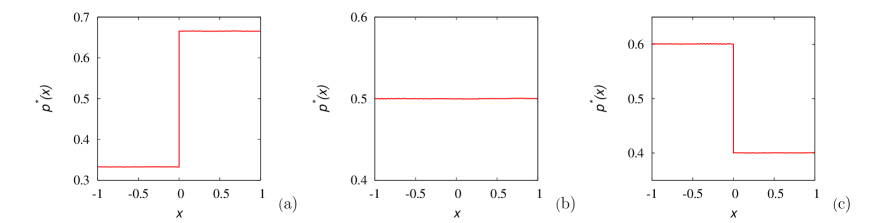
Figure 9: Stationary concentration profiles $p^{*}(x)$ vs $x$ at $\delta_{1}/\delta_{2}=2$. Panel (a) refers to $\tau_{2}=\tau_{1}$, (b) to $\tau_{2}=\tau_{1}/2$, (c) to $\tau_{2}=\tau_{1}/3$.

Indicate with $p_{1}(t)$ the fraction of particles at time $t$ within phase “1”. The dynamics of this quantity, relaxing towards $p_{1}^{*}$ (depicted in figure 4 of the main text), is shown in figure 10 for $\delta_{2}=\delta_{1}$, at several values of $\tau_{2}$. The data have been reported using the normalized abscissa $D_{1}\,t$. Since $\delta_{1}=1/N$, $N=100$, $\tau_{1}=1$, $D_{1}=5\times 10^{-5}$ a.u.

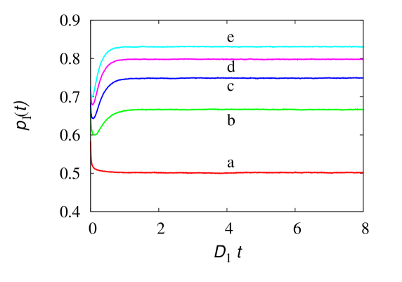
Figure 10: $p_{1}(t)$ vs $t$ in a closed MuPh-LRW cell at $\delta_{2}=\delta_{1}$ for several values of $\tau_{2}$: from (a) to (e), $\tau_{2}=\tau_{1}/h$, $h=1,2,3,4,5$.

Boundary conditions

The boundary conditions for MuPh-LRW in the presence of ideal interfaces can be derived in several different ways. In a fully lattice description, MuPh-LRW is solely a simple symmetric walk on ${\mathbb{Z}}$ parametrized with respect to the lattice time $n\in{\mathbb{N}}$. Its statistical description involves the probabilities $P_{h}^{n}$ of finding the particle at the lattice site $h$ at the lattice time $n$, fulfilling the Markov dynamics $P_{n}^{h+1}=(P_{h-1}^{n}+P_{h+1}^{n})/2$.

In a spatially continuous representation of the process, when positions $x\in{\mathbb{R}}$, the spatial heterogeneity, associated with the different values of $\delta_{h}$ in the two lattice phases plays a role. Let $p(x,n)$ the probability density function continuously parametrized with respect to the spatial coordinate $x$. The probability $P_{h}^{n}$ corresponds to the integral of the continuous $p(x,n)$ over an interval centered at $x_{h}$ of width $\delta_{\sigma(x_{h})}$, where $\sigma(x_{h})=1,2$, depending whether the site belongs to phase “1” or “2”., Consequently,

$$P_{h}^{n}\simeq p(x_{h},n)\,\delta_{\sigma(x_{h})}$$ (13)

The hyperbolic stochastic model associated with $p(x,n)$, taking a continuation of $n$ towards real values, stems from a local stochastic dynamics given by

$$dx(n)=\delta(x)\,(-1)^{\chi(n,1)}\,dn$$ (14)

where $\delta(x)=\delta_{1}$ if $\sigma(x)=1$, and $\delta(x)=\delta_{2}$ if $\sigma(x)=2$, and the transition rate equals $1$.

Henceforth, let $\Omega_{1}$, $\Omega_{2}$ be the subset of ${\mathbb{R}}$, $\Omega_{1}\cup\Omega_{2}={\mathbb{R}}$ , occupied by phase “1” and phase “2”, respectively, and let $p_{\pm}^{(h)}(x,n)$ the probability densities in the two lattice phases, $h=1,2$.

The hyperbolic hydrodynamic model expressed with respect to the continuation of the lattice time $n$ towards real values is given by

$$\frac{\partial p_{\pm}^{(h)}(x,n)}{\partial n}=\mp\delta_{h}\,\frac{\partial p_{\pm}^{(h)}(x,n)}{\partial x}\mp\left[p_{+}^{(h)}(x,n)-p_{-}^{(h)}(x,n)\right]\qquad x\in\Omega_{h}$$ (15)

Next, account for the time subordination of $t$ with respect to $n$,

$$dt=\tau(x)\,dn$$ (16)

where

$$\tau(x)=\left\{\begin{array}[]{ccc}\tau_{1}&&\in\Omega_{1}\\ \tau_{2}&&\in\Omega_{2}\end{array}\right.$$ (17)

which, in the present case of hyperbolic stochastic dynamics, means

$$\frac{\partial}{\partial n}=\frac{dt}{dn}\,\frac{\partial}{\partial t}$$ (18)

Consequently, with respect to the physical time $t$, the balance equations (15) becomes

$$\frac{\partial p_{\pm}^{(1)}(x,t)}{\partial t} = \mp b_{1}\frac{\partial p_{\pm}^{(1)}(x,t)}{\partial t}\mp\lambda_{1}\,\left[p_{+}^{(1)}(x,t)-p_{-}^{(1)}(x,t)\right]\qquad x\in\Omega_{1}$$

$$\frac{\partial p_{\pm}^{(2)}(x,t)}{\partial t} = \mp b_{2}\frac{\partial p_{\pm}^{(2)}(x,t)}{\partial t}\mp\lambda_{2}\,\left[p_{+}^{(2)}(x,t)-p_{-}^{(2)}(x,t)\right]\qquad x\in\Omega_{2}$$ (19)

where $b_{h}=\delta_{h}/\tau_{h}$, $\lambda_{h}=1/\tau_{h}$, which is the model considered in the main text. The boundary condition at an ideal interface follows from the hyperbolic structure of eq. (19) by imposing that there is no singularity at the interface (alternatively, one can invoke steady-state conditions). To this purpose, instead of eq. (19) let us consider a mollified version of it, by defining a smooth velocity field $b(x;\varepsilon)$, which is $C^{k}({\mathbb{R}})$, with $k\geq 1$ with respect to $x$ for any $\varepsilon>0$, and such that, in the limit for $\varepsilon\rightarrow 0$, it reproduces the discontinuity in the lattice phase velocities,

$$\lim_{\varepsilon\rightarrow 0}b(x;\varepsilon)=\left\{\begin{array}[]{ccc}b_{1}&&x\in\Omega_{1}\\ b_{2}&&x\in\Omega_{2}\end{array}\right.$$ (20)

and similarly for the transition rates $\lambda_{h}$, introducing a smooth field $\lambda(x;\varepsilon)$. With respect to this mollified description, eq. (19) becomes

$$\frac{\partial p_{\pm}(x,t)}{\partial t}=\mp\frac{\partial\left[b(x;\varepsilon)\,p_{\pm}(x,t)\right]}{\partial x}-\lambda(x;\varepsilon)\,\left[p_{+}(x,t)-p_{-}(x,t)\right]$$ (21)

Let $x_{0}$ be the position of an ideal interface. Integrating eq. (21) in the interval $[x_{0}-\eta,x_{0}+\eta]$, where $\varepsilon>0$ is a small parameter, one obtains

$$\pm\left[b(x_{0}+\eta;\varepsilon)\,p_{\pm}(x_{0}+\eta,t)-b(x_{0}-\eta;\varepsilon)\,p_{\pm}(x_{0}-\eta,t)\right]=-\int_{x_{0}-\eta}^{x_{0}+\eta}\frac{\partial p_{\pm}(x,t)}{\partial t}\,dx$$

$$-\int_{x_{0}-\eta}^{x_{0}+\eta}\lambda(x;\varepsilon)\,\left[p_{+}(x,t)-p_{-}(x,t)\right]\,$$ (22)

and let

$$Dp_{\rm max} = \max_{x\in[x_{0}-\eta,x_{0}+\eta]}\left|\frac{\partial p_{\pm}(x,t)}{\partial t}\right|\,,\qquad\lambda_{\rm max}=\max_{x\in[x_{0}-\eta,x_{0}+\eta]}\lambda(x;\varepsilon)\$$

$$\Delta_{\rm max} = \max_{x\in[x_{0}-\eta,x_{0}+\eta]}\left|p_{+}(x,t)-p_{-}(x,t)\right|$$ (23)

All these quantities can be assumed to be finite, at least for sufficiently long timescales. Consequently,

$$|b(x_{0}+\eta;\varepsilon)\,p_{\pm}(x_{0}+\eta,t)-b(x_{0}-\eta;\varepsilon)\,p_{\pm}(x_{0}-\eta,t)|\leq 2\,\eta\left[Dp_{\rm max}+\lambda_{\rm max}+\Delta_{\rm max}\right]$$ (24)

and, in the limit for $\eta\rightarrow 0$, one recovers

$$b(x_{0}^{-};\varepsilon)\,p_{\pm}(x_{0}^{-},t)=b(x_{0}^{+};\varepsilon)\,p_{\pm}(x_{0}^{+},t)$$ (25)

Taking the limit for $\varepsilon\rightarrow 0$, the velocity-based boundary condition follows

$$b_{1}\,p_{\pm}^{(1)}(x_{0},t)=b_{2}\,p_{\pm}^{(2)}(x_{0},t)$$ (26)

introduced in the main text.

It is possible to provide a lattice-dynamics based analysis of the interfacial boundary conditions leading to eq. (26) generalizing the approach developed by Ovaskainen and Cornell [23] which derive the same boundary condition in Appendix A.1 Case A (in the case of pure spatial heterogeneity). In point of fact, in the Ovaskainen and Cornell paper, the symmetric case of an ideal interface considered in the present work corresponds to $z=0$ in their calculations, and the quantities $q_{\pm}$ used in their analysis are proportional to $\delta_{h}$, $h=1,2$.

Dispersion in a periodic MuPh-LRW structure

The data for the effective diffusion coefficient $D_{\rm eff}$ reported in the main text, refer to the long-term emergent behavior observed in particle motion in a periodic multiphase lattice. The unit cell considered is the same used for closed-system numerical experiments, consisting of $N_{1}=100$ sites for phase “1” and $N_{2}=\alpha\,N_{1}$ sites for phase “2” where $\alpha$ is defined by $\delta_{2}=\delta_{1}/\alpha$.

Figure 11 depicts a portion of a trajectory of a lattice particle moving in a multiphase periodic lattice, in the rather extreme situation $\delta_{2}=\delta_{1}/10$, $\tau_{2}=\tau_{1}$.

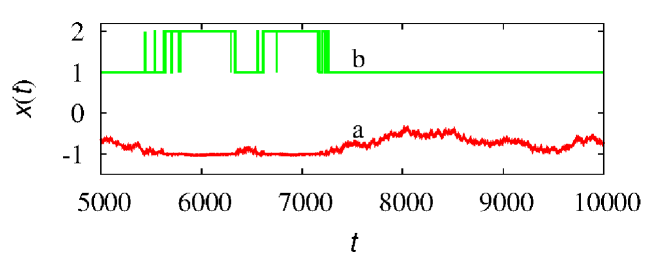
Figure 11: Portion of a trajectory (line a) of a lattice particle in a multiphase periodic lattice at $\delta_{2}=\delta_{1}/10$, $\tau_{2}=\tau_{1}$. Line (b) indicates the phase of the site at which the particle is located at time $t$.

The results for $D_{\rm eff}$ stem from the long-term linear scaling with time of the mean square displacement $\sigma_{x}^{2}(t)$, that fulfils the emergent Einsteinian behavior

$$\sigma_{x}^{2}(t)\sim 2\,D_{\rm eff}\,t\qquad D_{1}t\gg 1$$ (27)

as depicted in figure 12 at $\delta_{2}=\delta_{1}$ for several values of the ratio $\tau_{2}/\tau_{1}$.

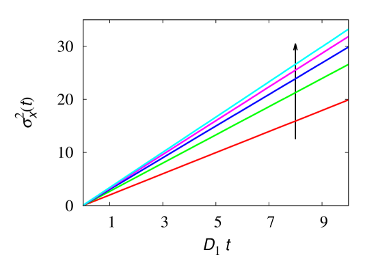
Figure 12: Mean square displacement $\sigma_{x}^{2}(t)$ vs $D_{1}t$ for particle motion in a MuPh-LRW periodic lattice at $\delta_{2}=\delta_{1}$ for several values of $\tau_{2}=1/h$, $h=1,\dots,5$, ($\tau_{1}=1$). The arrow indicates increasing values of $h$.

The continuous hydrodynamic model for MuPh-LRW in periodic lattices stems from a space-time continuous description of stochastic particle motion in the presence of ideal interfaces. Since an ideal interface does not exert any specific active contribution to random particle dynamics, but neutrally separates the two lattice phases, it is intuitive that continuous hydrodynamic models should be derived from simple stochastic motion on ${\mathbb{R}}$ in a time-continuous setting, in which the heterogeneity in transport parameters, deriving from the multiphase partition of the lattice, is accounted for.

As discussed in the previous paragraphs, the continuous hyperbolic hydrodynamic model is just the evolution equation for the statistical description, expressed by mean of the partial probability waves, of the Poisson-Kac process

$$dx(t)=b(x(t))\,(-1)^{\chi(t;\lambda(x(t)))}\,dt$$ (28)

where the functions $b(x)$ and $\lambda(x)$ are expressed by

$$b(x)=\left\{\begin{array}[]{ccc}b_{1}=\delta_{1}/\tau_{1}&&x\in\Omega_{1}\\ b_{2}=\delta_{2}/\tau_{2}&&x\in\Omega_{2}\end{array}\right.\,,\qquad\lambda(x)=\left\{\begin{array}[]{ccc}1/\tau_{1}&&x\in\Omega_{1}\\ 1/\tau_{2}&&x\in\Omega_{2}\end{array}\right.$$ (29)

This model gives rise to the hydrodynamic equations (19) equipped with the interfacial conditions (26), out of which the expression for the effective diffusion coefficient reported in the main text, and here rewritten, follows (assuming equal fractions of the two lattice phases, i.e., $L_{1}=L_{2}$) [26]

$$\frac{1}{D_{\rm eff}}=\frac{1}{2}\left(\frac{1}{b_{1}}+\frac{1}{b_{2}}\right)\left(\frac{1}{b_{1}\,\tau_{1}}+\frac{1}{b_{2}\,\tau_{2}}\right)$$ (30)

A parabolic model for MuPh-LRW stems from the statistical properties of a Langevin equation for particle dynamics

$$dx(t)=\sqrt{2\,D(x)}*_{\lambda}dw(t)$$ (31)

driven by the increments $dw(t)$ of a Wiener process in the time interval $dt$, and “$*_{\lambda}$”, $\lambda\in[0,1]$, indicates that a $\lambda$-calculus has been chosen for the stochastic integrals (where $\lambda=0$ provides the Ito, $\lambda=1/2$ the Stratonovich, and $\lambda=1$ the Hänggi-Klimontovich representations).

In eq. (31), $D(x)$ is the local diffusivity that depends on position due to phase heterogeneity and periodicity

$$D(x)=\left\{\begin{array}[]{ccc}D_{1}=\delta_{1}^{2}/2\,\tau_{1}&&x\in\Omega_{1}\\ D_{2}=\delta_{2}^{2}/2\,\tau_{2}&&x\in\Omega_{2}\end{array}\right.$$ (32)

Consequently eq. (31) is a highly nonlinear Langevin equation, with discontinuous coefficients, and its properties can be studied by considering a mollified version of it,

$$dx(t)=\sqrt{2\,\widetilde{D}(x;\varepsilon)}*_{\lambda}dw(t)$$ (33)

by introducing $\widetilde{D}(x;\varepsilon)$, $\varepsilon>0$ that represents a family of smooth $C^{k}({\mathbb{R}})$ fields, $k\geq 1$, that in the limit for $\varepsilon\rightarrow 0$ converge to the discontinuous diffusivity profile expressed by eq. (32),

$$\lim_{\varepsilon\rightarrow 0}\widetilde{D}(x;\varepsilon)=D(x)$$ (34)

We are considering all the possible stochastic integrals, i.e., all the values of $\lambda\in[0,1]$, in order to test the capability of a Langevin-Wiener stochastic models to describe the long-term properties of a MuPh-LRW. Of course, the choice of $\lambda$ implicitly determines the boundary condition at the interfacial points separating the two lattice phases.

The long term properties of the stochastic motion defined by (31) can be obtained from the homogenization analysis of the associated Fokker-Planck equation, and provide the following expression for the effective diffusivity [26]

$$\frac{1}{D_{\rm eff}}=\frac{1}{4}\left(\frac{1}{D_{1}^{1-\lambda}}+\ \frac{1}{D_{2}^{1-\lambda}}\right)\left(\frac{1}{D_{1}^{\lambda}}+\ \frac{1}{D_{2}^{\lambda}}\right)$$ (35)

It has been shown in the main text that the hyperbolic model provides the correct behavior of the effective diffusivity for a MuPh-LRW in the presence of ideal interfaces over all the range of lattice parameters, while this is not the case for the parabolic models based on the continuous space-time approximation of stochastic motion via eq. (31).

Figure 13 complements the data shown in the main text. It provides the comparison of the effective diffusivity obtained for the hyperbolic model eq. (30) (coinciding with that of found in lattice simulations of MuPh-LRW dispersion), with the diffusivities deriving from the Langevin-Wiener model eq. (35) at different values of $\lambda$, for typical conditions. First of all, observe from eq. (35) that $D_{\rm eff}|_{\lambda}=D_{\rm eff}|_{1-\lambda}$, thus the Ito and the Hänggi-Klimontovich approaches to stochastic motion provide the same long-term dispersive behavior.

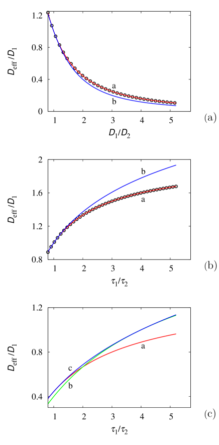
Figure 13: Comparison of $D_{\rm eff}/D_{1}$ for the continuous models of particle motion in multiphase lattices. In all the panels, lines (a) correspond to the results deriving from the hyperbolic model. Panel (a) refers to $\tau_{2}=\tau_{1}$, $\delta_{2}\neq\delta_{1}$: symbols ($\circ$) correspond to the Langevin-Stratonovich, and line (b) to the Langevin-Ito models, respectively. Panel (b) refers to $\delta_{1}=\delta_{2}$, in the case $\tau_{2}\neq\tau_{1}$: symbols ($\circ$) correspond to the Langevin-Ito, and line (b) to the Langevin-Stratonovich models, respectively. Panel (c): general case, $\delta_{2}\neq\delta_{1}$, $\tau_{2}\neq\tau_{1}$, in the case the ratio of the diffusivity is fixed to $D_{1}/D_{2}=2$. Line (b) corresponds to the Langevin-Ito, and line (c) to the Langevin-Stratonovich models, respectively.

From the functional structure of the expressions (30) and (35) it follows that:

• if the lattice heterogeneity involves solely the spatial parameters, i.e., $\tau_{1}=\tau_{2}$, then the Langevin-Stratonovich approximation provides the correct expression for the effective diffusion coefficient, as depicted in panel (a) of figure 13;

• if the lattice heterogeneity involves the timescales, i.e., $\delta_{1}=\delta_{2}$, the Langevin-Ito (or equivalently the Hänggi-Klimontovich interpretation) provides the right value of $D_{\rm eff}$ as depicted in panel (b) of figure 13;

• in the case both spatial and time scales in the two lattice phases are different, there is no parabolic model stemming from a Langevin-Wiener approximation of the lattice dynamics that yields the correct long-term behavior found in numerical experiments of MuPh-LRW. This phenomenon is depicted in panel (c) of figure 13.

Qualitative analysis

It can be useful to explore further the properties of the expressions for the effective diffusivities. To begin with, consider the parabolic approximation, i.e., eq. (35). In this case, the ratio $D_{\rm eff}/D_{1}$ depends solely on the ratio $\gamma=D_{1}/D_{2}$ of the diffusivities in the two lattice phases

$$\frac{D_{1}}{D_{\rm eff}}=\frac{1}{4}\left[1+\gamma^{1-\lambda}+\gamma^{\lambda}+\gamma\right]=\frac{1}{\zeta(\gamma,\lambda)}$$ (36)

The function $\zeta(\gamma,\lambda)$, for fixed $\gamma$, attains its maximum value at $\lambda=1/2$, and consequently the Stratonovich interpretation provides the maximum value of the effective diffusivity, see figure 14.

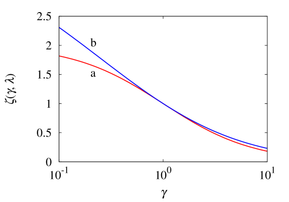
Figure 14: Behavior of the function $\zeta(\gamma,\lambda)$ as a function of the ratio $\gamma$ of the two lattice phase diffusivities. Line (a) refers to $\lambda=0$ (Ito), line (b) to $\lambda=1/2$ (Stratonovich).

Specifically,

$$\zeta(\gamma,0)=\frac{2}{1+\gamma}\,,\qquad\zeta\left(\gamma,\frac{1}{2}\right)=\frac{4}{(1+\sqrt{\gamma})^{2}}$$ (37)

Next, consider the hyperbolic model. Introducing the nondimensional group $\beta=b_{1}/b_{2}$, corresponding to the ratio of the lattice velocities in the two phases, eq. (30) can be expressed as

$$\frac{D_{1}}{D_{\rm eff}}=\frac{1}{4}\left[(1+\beta)+\gamma\left(1+\frac{1}{\beta}\right)\right]=h(\gamma,\beta)$$ (38)

The function $h(\gamma,\beta)$ is depicted in figure 15 as a function of its second argument $\beta$.

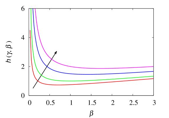
Figure 15: $h(\gamma,\beta)$ as a function of $\beta$ for several values of $\gamma=0.5,\,1,\,2,\,3$. The arrow indicates increasing values of $\gamma$.

The function $h(\gamma,\beta)$, for fixed $\gamma$, attains its local extremal value at $\beta^{*}$ (local minimum) given by

$$\beta^{*}=\sqrt{\gamma}$$ (39)

and the corresponding value of $D_{1}/D_{\rm eff}^{*}$ is given by

$$\frac{D_{1}}{D_{\rm eff}^{*}}=\frac{(1+\sqrt{\gamma})^{2}}{4}$$ (40)

coinciding with the results obtained in the Langevin-Stratonovich case. It follows from this observation that, for fixed $\gamma$, i.e., for fixed values of the lattice phase diffusivities, the maximum value of the effective diffusivity in MuPh-LRW dispersion obtained by varying the ratio $\beta$ between the lattice velocities is provided by the Langevin-Stratonovich dispersion coefficient, i.e.,

$$\left.\frac{D_{\rm eff}^{\mbox{MuPh-LRW}}(\beta)}{D_{1}}\right|_{\mbox{fixed}\;\gamma}\leq\,\frac{D_{\rm eff}^{\mbox{Strato}}(\gamma)}{D_{1}}$$ (41)

References

- [1] P. L. Krapivsky, S. Redner and E. Ben-Naim A Kinetic View of Statistical Physics (Cambridge University Press, Cambridge, 2010).
- [2] H. Kleinert Gauge Fields in Condensed Matter (World Scientific, Singapore, 1989).
- [3] A. De Masi and E. Presutti Mathematical Methods for Hydrodynamic Limits (Springer-Verlag, Berlin, 1991).
- [4] C. Kipnis and C. Landim Scaling Limits of Interacting Particle Systems (Springer-Verlag, Berlin, 1999).
- [5] H. Scher and M. Lax, Phys. Rev. B 7, 4491 (1973).
- [6] G. H. Weiss, J. Stat. Phys. 15, 157 (1976).
- [7] G. H. Weiss Aspects and Applications of the Random Walk (North-Holland, Amsterdam, 1994).
- [8] D. ben-Avraham and S. Havlin, Diffusion and Reactions in Fractals and Disordered Systems (Cambridge University Press, Cambridge, 2000).
- [9] H. Scher and E. Montroll, Phys. Rev. B 12, 2455 (1975).
- [10] J. Klafter and R. Silbey, Phys. Rev. Lett. 44, 55 (1980).
- [11] N. Korabel and E. Barkai, Phys. Rev. E 83, 051113 (2011).
- [12] N. Korabel and E. Barkai, Phys. Rev. Lett. 104, 170603 (2010).
- [13] M. Marseguerra and A. Zoia, Ann. Nuclear Energy 33, 1396 (2006).
- [14] T. Kosztolowicz, J. Membrane Sci. 320, 492 (2008)
- [15] J. Alvarez-Ramirez, I. Dagdug and M. Meraz, Physica A, 395, 193 (2014).
- [16] P. K. Ghosh, Y. Li, F. Marchesoni and F. Nori, Phys. Rev. E 92, 012114 (2015).
- [17] O. Farago and N. Grombech-Jensen, Phys. Rev. E 89, 013301.
- [18] Y. Tang, R. Yuan, J. Chen and P. Ao, Phys. Rev. E 90, 052121 (2014).
- [19] P. F. Tupper and X. Yang, Proc. R. Soc. A, rspa.2012.0259 (2012).
- [20] M. Giona, Lattice Random Walk: an old problem with a future ahead, Phys. Scripta (2018), submitted.
- [21] M. Giona, A. Brasiello and S. Crescitelli, J. Non-Equil. Thermodyn. 41, 107 (2016).
- [22] M. Giona, A. Brasiello and S. Crescitelli, J. Phys. A 50, 335002 (2017).
- [23] O. Ovaskainen and S.J. Cornell, J. Appl. Prob. 40, 557 (2003).
- [24] M. Giona, A. Brasiello and S. Crescitelli, J. Phys. A 50, 335003 (2017).
- [25] M. Giona, A. Brasiello and S. Crescitelli, J. Phys. A 50, 335004 (2017).
- [26] M. Giona and D. Cocco, Homogenization Approaches to Multiphase Lattice Random Walks, submitted to ArXiv (2018).
- [27] P. Kloeden and E. Platen, Numerical Solution of Stochastic Differential Equations (Springer Verlag, Berlin, 1995).
- [28] P. N. Pusey, Science 332, 802 (2011).
- [29] T. Li and M. G. Raizen, Ann. Phys. (Berlin) 525, 281 (2013).
- [30] A. Striolo, NanoLetters 6, 633 (2006).
- [31] K. S. Novoselov, A. K. Geim, S. V. Morozov, D. Jiang, M. I. Katsnelson, I. Grigorieva, S. V. Dubonos and A. A. Firson, Nature 438, 197 (2005).
- [32] S. Das Sarma, S. Adam, E.H. Hwang and E. Rossi, Rev. Mod. Phys. 83, 407 (2011).