Several recent developments in estimation and robust control of quantum systems*

Abstract

This paper summarizes several recent developments in the area of estimation and robust control of quantum systems and outlines several directions for future research. Quantum state tomography via linear regression estimation and adaptive quantum state estimation are introduced and a Hamiltonian identification algorithm is outlined. Two quantum robust control approaches including sliding mode control and sampling-based learning control are illustrated.

I INTRODUCTION

Quantum technology has shown powerful potential for developing future technology [1]. Practical applications of quantum technology include secure quantum communication, powerful quantum computation and high-precision quantum metrology. These potential applications have attracted many mathematicians, physicists, computer scientists and control engineers to this booming field.

A fundamental task in quantum technology is to characterize the state of a quantum system and identify the parameters in the system. The estimation procedure of a static quantum state is often referred as quantum state tomography [1]. For estimating a dynamical state, quantum filtering theory [2, 3] has been developed, which is especially useful for addressing the measurement-based quantum feedback control problem [4]. The area of identifying key parameters in quantum systems can be referred as quantum system identification [5]. Another important problem is robustness of quantum systems in developing practical quantum technology since real quantum systems are often subject to noises, incomplete knowledge or uncertainties [6]. In this paper, we introduce some recent developments in the areas of estimation and robust control of quantum systems. We do not intend to survey the main progress in these areas. Instead, we present several examples and methods that were recently developed by the authors and their collaborators, and aim to illustrate several classes of significant quantum estimation and control problems as well as outline open questions for future research.

This paper is organized as follows. In Section II we introduces quantum state tomography via linear regression estimation and adaptive quantum state tomography. Section III presents the identification problem of quantum processes and system Hamiltonian. Section IV outlines two quantum robust control methods including sliding mode control and sampling-based learning control. Conclusions are presented in Section V.

II Quantum state estimation

II-A Quantum state tomography

Quantum state tomography provides a framework to reconstruct quantum states. The state of a quantum system can be described by a density matrix $\rho$ which is a Hermitian, positive semidefinite matrix satisfying $\text{Tr}(\rho)=1$. A pure state can also be described by a unit complex vector $|\psi\rangle$ with $\rho=|\psi\rangle\langle\psi|$ [1]. A mixed state is linear combination of independent pure states. To estimate a quantum state, we usually need to make measurements on many copies of the state. For quantum measurement, a set $\{P_{i}\}$ of positive operator valued measurement (POVM) elements is prepared (e.g., mutually unbiased basis [7]), where $P_{i}\geq 0$ and $\sum_{i}P_{i}=I$ with $I$ being the identity matrix. The occurrence probability of the $i$th outcome can be calculated as $p_{i}=\text{Tr}(\rho P_{i})$ according to the Born Rule, where $\text{Tr}(A)$ returns the trace of the matrix $A$. For a given unknown quantum state, we need to design POVM measurement and develop an estimation algorithm to reconstruct the quantum state from measurement data. Various quantum state tomography methods have been developed such as maximum likelihood estimation (MLE) method [8]-[10], Bayesian mean estimation approach [11, 12] and linear regression estimation (LRE) [13]. For more details of MLE and Bayesian mean estimation, please refer to [8, 11]. Here we only introduce the LRE method recently developed for quantum state tomography.

II-B Quantum state tomography via LRE

In the LRE framework, the reconstruction problem of a quantum state can first be converted into a parameter-estimation problem of a linear regression model [13]. Consider a $d$-dimensional quantum system associated with Hilbert space $\mathcal{H}$. Let $\{\Omega_{i}\}^{d^{2}-1}_{i=1}$ denote a set of Hermitian operators satisfying (i) $\textmd{Tr}(\Omega_{i})=0$ and (ii) $\textmd{Tr}(\Omega_{i}\Omega_{j})=\delta_{ij}$, where $\delta_{ij}$ is the Kronecker function. The quantum state $\rho$ to be reconstructed can be parameterized as

$$\rho=\frac{I}{d}+\sum^{d^{2}-1}_{i=1}\theta_{i}\Omega_{i},$$

where $\theta_{i}=\textmd{Tr}(\rho\Omega_{i})$. Let $\Theta=(\theta_{1},\cdots,\theta_{d^{2}-1})^{T}$, where $T$ denotes the transpose operation. Then we parameterize the quantum measurements. Suppose a series of quantum measurements $\{E^{(j)}\}^{M}_{j=1}$ are performed. Then each operator $E^{(j)}$ can be parameterized under bases $\{\Omega_{i}\}^{d^{2}-1}_{i=1}$ as [14]

$$E^{(j)}=\frac{\gamma^{(j)}_{0}}{d}+\sum^{d^{2}-1}_{i=1}\gamma^{(j)}_{i}\Omega_{i},$$

where $\gamma^{(j)}_{0}=\textmd{Tr}(E^{(j)})$ and $\gamma^{(j)}_{i}=\textmd{Tr}(E^{(j)}\Omega_{i})$. Let $\Gamma^{(j)}=(\gamma^{(j)}_{1},\cdots,\gamma^{(j)}_{d^{2}-1})^{T}$. When we make measurements on many identical copies of a quantum system in the state $\rho$, the probability of obtaining the result of $E^{(j)}$ can be calculated as

$$p(E^{(j)})=\textmd{Tr}(E^{(j)}\rho)=\frac{\gamma^{(j)}_{0}}{d}+\Theta^{T}{\Gamma^{(j)}}.$$ (1)

Suppose that we perform $E^{(j)}$ measurements for $n^{(j)}$ times with positive results $n^{(j)}_{1}$ times, where $\sum_{j}^{M}n^{(j)}=N$ for the total number of copies $N$. Denote $\hat{x}$ the estimator of $x$. Let $\hat{p}(E^{(j)})=n^{(j)}_{1}/n^{(j)}$, and $e^{(j)}=\hat{p}(E^{(j)})-p(E^{(j)})$. Using (1), the following linear regression equations can be obtained for $j=1,\ \cdots,M$,

$$\hat{p}(E^{(j)})=\frac{\gamma^{(j)}_{0}}{d}+{\Gamma^{(j)}}^{T}\Theta+e^{(j)}.$$ (2)

Now, if we obtain the solution $\Theta$, the quantum state $\rho$ can be reconstructed. We rewrite (2) as

$$Y_{M}=X_{M}\Theta+{{\bf{e}}_{M}}$$ (3)

where

$$Y_{M}=(\hat{p}(E^{(1)})-\frac{1}{d},\cdots,\hat{p}(E^{(n)})-\frac{1}{d},\cdots,\hat{p}(E^{(M)})-\frac{1}{d})^{T},$$

$$X_{M}=(\Gamma^{(1)},\cdots,\Gamma^{(n)},\cdots,\Gamma^{(M)})^{T}$$

and

$${{\bf{e}}_{M}}=(e^{(1)},\cdots,e^{(n)},\cdots,e^{(M)})^{T}.$$

We aim to find an estimate $\hat{\Theta}$ such that

$$\hat{\Theta}=\underset{\hat{\Theta}}{\text{argmin}}\sum_{j=1}^{M}W^{(j)}[\hat{p}(E^{(j)})-\frac{\gamma^{(j)}_{0}}{d}-{\hat{\Theta}}^{T}{\Gamma^{(j)}}]^{2},$$ (4)

where $W_{M}=\textmd{diag}(W^{(1)},\cdots,W^{(n)},\cdots,W^{(M)})^{T}$ represent the weights of different linear regression equations. It is straightforward to obtain the least-squares solution to (4). Once the solution is obtained, we can reconstruct a Hermitian matrix $\tilde{\rho}$ with $\textmd{Tr}\tilde{\rho}=1$. However, $\tilde{\rho}$ is not necessarily physical since measurement noise is unavoidable. The algorithm in [15] can be used to find a physical state $\hat{\rho}$ from $\tilde{\rho}$. The estimation error can be characterized using the mean squared error (MSE) $E\textmd{Tr}(\hat{\rho}-\rho)^{2}$, where $E(\cdot)$ indicates the expectation on all possible measurement outcomes.

An advantage of LRE for quantum state tomography is that its computational complexity can be characterized and the theoretical error upper bound may be obtained. In [13], its computational complexity $O(d^{4})$ for estimating a $d$-dimensional quantum state has been proven and numerical results showed that the LRE algorithm is around 10000 times faster than the MLE approach for quantum state estimation. The LRE algorithm can be further optimized and implemented on GPU, and such improvement has demonstrated the realization of reconstructing a 14-qubit state using only 3.35 hours [16].

II-C Adaptive quantum state estimation

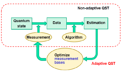
Figure 1: Schematic of adaptive quantum state tomography (QST)

Another advantage of LRE is that it is suitable for developing adaptive quantum state estimation method. Adaptive protocols [17]-[21] have been proven to have the capability to improve the quantum estimation precision. In adaptive state estimation as shown in Figure 1, we first make measurements on part of copies and get a rough estimate of the quantum state. Then we find optimal measurement bases to make measurements on some other copies. It may involve multiple steps of adaptivity according to practical tasks.

In LRE, equation (4) can be recursively solved. Define

$$\begin{array}[]{c}Q_{n}=(\sum^{n}_{k=1}W^{(k)}\Gamma^{(k)}{\Gamma^{(k)}}^{T})^{-1},\\ a_{n}=(\frac{1}{W^{(n)}}+{{\Gamma^{(n)}}^{T}}Q_{n-1}\Gamma^{(n)})^{-1}.\end{array}$$ (5)

For $n=1,\cdots,M$, we have [14]

$$Q_{n}=Q_{n-1}-a_{n}Q_{n-1}\Gamma^{(n)}{{\Gamma^{(n)}}^{T}}Q_{n-1}.$$ (6)

$\hat{\Theta}_{n}$ can be recursively calculated as

$$\hat{\Theta}_{n}=\hat{\Theta}_{n-1}+a_{n}Q_{n-1}\Gamma^{(n)}(\hat{p}(E^{(n)})-\frac{\gamma^{(n)}_{0}}{d}-{{\Gamma^{(n)}}^{T}}\hat{\Theta}_{n-1}).$$ (7)

Using (6) and (7), one can recursively incorporate new measurement data into historical measurement data, which provides a convenient way for adaptive estimation of $\rho$. In this sense, the LRE method is more suitable for adaptive reconstruction of quantum states due to its recursive procedure than traditional MLE or Bayesian mean method. In the LRE framework, instead of repeatedly calculating all the historical data when new data arrive, we only need to add the new data into historical information matrix and vector, which significantly reduces the calculation cost.

We need to design a criterion to optimize the measurement bases at each adaptive step. In [14], Qi et al. illustrated that when the resource number $N$ becomes large enough, $E(\hat{\Theta}_{n}-\Theta)(\hat{\Theta}_{n}-\Theta)^{T}\approx Q_{n}$. Based on the observation, an adaptive quantum state tomography protocol has been developed in [14]. In the first stage, one performs a standard LRE on $N_{1}$ copies with the standard cube measurement bases to obtain a preliminary $\hat{\Theta}$ and $Q$. In the second stage, the initial values of $Q$ in (6) and $\hat{\Theta}$ in (7) are set as $Q_{0}=Q$ and $\hat{\Theta}_{0}=\hat{\Theta}$, and then the remaining $N-N_{1}$ copies are utilized for multi-step adaptive estimation. If the resource number is $N_{2}$ in each step and $K$ steps of adaptivity are used, then $N=N_{1}+K\cdot N_{2}$.

Suppose after $s$ steps, we have $Q_{s}$ and $\hat{\Theta}_{s}$. We define $\textbf{g}_{s+1}\equiv\textmd{Tr}Q_{s}-\textmd{Tr}Q_{s+1}$. According to the experimental capability, if the candidate measurement basis set $\{E^{(s+1)}\}$ is finite, one can calculate $\textbf{g}_{s+1}$ for each candidate basis and pick up the one with the largest $\textbf{g}_{s+1}$ as the measurement basis at ($s+1$)-th step. When $\{E^{(s+1)}\}$ is an infinite set, one needs to either analytically find the optimal basis or try to obtain an approximate optimal basis. In [22], an analytical optimal solution has been provided for estimating a single-qubit state. For two-qubit states, a heuristic deduction to search for the optimal measurement bases was presented in [14], where numerical and experimental results showed that the adaptive quantum state tomography can improve the estimation precision.

II-D Discussion

Many problems remain open in the area of quantum state tomography. For example, the efficiency of the estimation algorithms may be further enhanced if there is prior knowledge on the quantum state to be reconstructed. Various variants of LRE could be developed for quantum state tomography and different adaptivity criteria can be explored for adaptive estimation of quantum states. The capability of parallel processing for quantum state estimation and the precision limit of adaptive estimation are worth further exploring. Moreover, new approaches such as coherent observers [23, 24] and machine learning methods may provide different angles for estimating the state of a quantum system.

III Quantum system identification

III-A Quantum Process Tomography

We illustrate the general framework of quantum process tomography described in [1, 25, 26]. A quantum process $\varepsilon$ maps an input state $\rho_{in}$ to an output state $\rho_{out}$. In Kraus operator-sum representation [1], we have

$$\varepsilon(\rho_{in})=\rho_{out}=\sum_{i}A_{i}\rho_{in}A_{i}^{\dagger},$$ (8)

where $A^{\dagger}$ is the conjugation ($*$) and transpose ($T$) of $A$ and $\{A_{i}\}$ is a set of $d\times d$ matrices, with $\sum_{i}A_{i}^{\dagger}A_{i}\leq I$. We usually focus on trace-preserving operations, which means satisfying the completeness relation

$$\sum_{i}A_{i}^{\dagger}A_{i}=I.$$ (9)

By expanding $\{A_{i}\}$ in a fixed family of basis matrices $\{F_{i}\}$, we obtain $A_{i}=\sum_{j}c_{ij}F_{j}$, and $\varepsilon(\rho_{in})=\sum_{jk}F_{j}\rho_{in}F_{k}^{\dagger}x_{jk}$, with $x_{jk}=\sum_{i}c_{ij}c_{ik}^{*}$. If we take matrix $C=[c_{ij}]$, $X=[x_{ij}]$, then $X=C^{T}C^{*}$, which indicates $X$ is Hermitian and positive semidefinite. $X$ is called process matrix [27]. $X$ and $\varepsilon$ are one-to-one correspondent. Hence, we can obtain the full characterization of $\varepsilon$ by reconstructing $X$. The completeness constraint (9) now is $\sum_{j,k}x_{jk}F_{k}^{\dagger}F_{j}=I$.

Let $\{\rho_{m}\}$ be a complete basis set of the space $\mathbb{C}_{d\times d}$ consisting of all $d\times d$ matrices. If $\{\rho_{m}\}$ are linear independent, then each output can be expanded uniquely as $\varepsilon(\rho_{m})=\sum_{n}\lambda_{mn}\rho_{n}$. We can establish the relationship $F_{j}\rho_{m}F_{k}^{\dagger}=\sum_{n}B_{mn,jk}\rho_{n}$. Hence, $\sum_{n}\sum_{jk}B_{mn,jk}\rho_{n}x_{jk}=\sum_{n}\lambda_{mn}\rho_{n}.$ From the linear independence of $\{\rho_{m}\}$, we have $\sum_{jk}B_{mn,jk}x_{jk}=\lambda_{mn}$. Let matrix $\Lambda=[\lambda_{mn}]$ and we arrange the elements $B_{mn,jk}$ into a matrix $B$:

$$B=\!\!\left(\!\!\begin{array}[]{*{6}{c}}B_{11,11}&B_{11,21}&\cdots&B_{11,12}&\cdots&B_{11,d^{2}d^{2}}\\ B_{21,11}&B_{21,21}&\cdots&B_{21,12}&\cdots&B_{21,d^{2}d^{2}}\\ \lx@intercol\dotfill\hfil\hfil\lx@intercol\\ B_{12,11}&B_{12,21}&\cdots&B_{12,12}&\cdots&B_{12,d^{2}d^{2}}\\ B_{22,11}&B_{22,21}&\cdots&B_{22,12}&\cdots&B_{22,d^{2}d^{2}}\\ \lx@intercol\dotfill\hfil\hfil\lx@intercol\\ B_{d^{2}d^{2},11}&B_{d^{2}d^{2},21}&\cdots&B_{d^{2}d^{2},12}&\cdots&B_{d^{2}d^{2},d^{2}d^{2}}\\ \end{array}\!\!\right)$$

We define the vectorization function as $\text{vec}(A_{m\times n})=[A_{11},A_{21},...,A_{m1},A_{12},...,A_{m2},...,A_{mn}]^{T}$. For square $A$ we define $\text{vec}^{-1}[\text{vec}(A)]=A$. We have the relationship

$$B\text{vec}(X)=\text{vec}(\Lambda).$$ (10)

Here $B$ is determined once the bases $\{F_{i}\}$ and $\{\rho_{m}\}$ are chosen, and $\Lambda$ is obtained from experimental data. In practice, direct inversion or pseudo-inversion of $B$ may fail to generate a physical estimation $\hat{X}$ due to noise or uncertainty. A central issue in quantum process tomography is to design an algorithm to find a physical estimation $\hat{X}$ such that $B\text{vec}(\hat{X})$ is close enough to $\text{vec}(\hat{\Lambda})$. MLE [28, 29] aims to find the most likely process that can generate the current data. Bayesian mean deduction [18, 30, 31] uses Bayes formula to generate a posterior probability distribution, and the expectation of this probability distribution is taken as the final estimation result. We will discuss Hamiltonian identification within the framework of quantum process tomography in the next subsection.

III-B Hamiltonian identification

For a closed quantum system, its evolution can be described by

$$\dot{\rho}=-\frac{\text{i}}{\hbar}(\rho H-H\rho)$$ (11)

where $\text{i}=\sqrt{-1}$, $\hbar$ is reduced Planck’s constant (we set $\hbar=1$ in the following) and $H$ is the system Hamiltonian. It is clear that identifying $H$ is a fundamental task in quantum systems. Some approaches have been developed for Hamiltonian identification. For example, a Hamiltonian identification method using measurement time traces has been proposed based on classical system identification theory [32] and it has also been used to experimentally identify the Hamiltonian in spin systems [33]. In [34], dynamical decoupling was employed for identifying parameters in the Hamiltonian.

Here we briefly introduce the Hamiltonian identification algorithm in [26]. For a closed quantum system, the state evolution can be written into $\rho_{out}=e^{-\text{i}Ht}\rho_{in}e^{\text{i}Ht}$. Compared with (8), it is clear that the unitary propagator $e^{-\text{i}Ht}$ is the only Kraus operator. Hence, $C$ is a row vector, and $X$ is of rank one. Now the semidefinite requirement is naturally satisfied. Let $X=gg^{\dagger}$ and $g=\text{vec}(G)$. We thus know $G$ must be unitary if we choose natural bases $\{|k\rangle,k=1,2,\dots\}$. Furthermore, from Theorem 2 in [26], $B$ is now unitary. Denote $\hat{D}=\text{vec}^{-1}(B^{\dagger}\text{vec}(\hat{\Lambda}))$. Hence we need to find a unitary $\hat{G}$ to minimize $||\text{vec}(\hat{G})\text{vec}(\hat{G})^{\dagger}-\hat{D}||$ where $||\cdot||$ is the matrix Frobenius norm. This problem can be solved using a two-step optimization approach. We first find an $\hat{S}$ to minimize $||\text{vec}(\hat{S})\text{vec}(\hat{S})^{\dagger}-\hat{D}||$ and then find a unitary $\hat{G}$ to minimize $||\text{vec}(\hat{G})\text{vec}(\hat{G})^{\dagger}-\text{vec}(\hat{S})\text{vec}(\hat{S})^{\dagger}||$. Then Schur decomposition can be used to obtain the $\hat{H}$ through the relationship $e^{-\text{i}\hat{H}t}=\hat{G}^{T}$. Further, the computational complexity $O(d^{6})$ is given and an upper bound of estimation error is also established in [26]. Numerical results show that the Hamiltonian identification algorithm has much lower computational complexity than the approach in [32]. In [35], it is shown that a more efficient algorithm with computational complexity $O(d^{3})$ can be developed if only input pure states are used.

III-C Discussion

Quantum system identification has been growing quickly in the last several years. A large number of challenging problems is waiting for exploring. For example, although several results on identifiability of quantum systems [36] have been presented, the identifiability of more general quantum systems was not investigated. Adaptive approaches were only applied to the identification problems of several simple quantum systems such as estimating the Hamiltonian parameter of a two-level system [37] and more adaptive algorithms could be developed to enhance the identification precision for quantum systems. Since the computational complexity of quantum system identification algorithm usually exponentially increases with the number of qubits, it is expected to develop more efficient identification algorithms for quantum parameter identification. Other new directions for future research include the mechanism identification of physical process [38] and the identification of quantum networks [39, 40] where the network topology could be taken advantaged of.

IV Quantum robust control

In recent years, robust control approaches have been developed to enhance the robustness performance in quantum systems. In particular, several robust control design approaches including $H^{\infty}$ control [41]-[44], small gain theorem and Popov method [45] have been extended to linear quantum systems. More detailed results on control of linear quantum systems can refer to [46, 47]. In this section, we briefly introduce two robust control design methods of sliding mode control (SMC) and sampling-based learning control (SLC) for quantum systems.

IV-A Sliding mode control

SMC approach is a useful robust control method in classical control theory and industrial applications. However, it cannot directly be applied to quantum systems since the measurement operation usually changes the state to be measured [48]. In [49]-[51], a series of results on SMC of quantum systems have been presented. In particular, a quantum system with Hamiltonian uncertainty $H_{\Delta}$ has been considered and the system evolves according to Schrödinger equation

$$\begin{array}[]{l}\text{i}|\dot{\psi}(t)\rangle=(H_{0}+H_{\Delta}+H_{u})|\psi(t)\rangle,\\ |\psi(t=0)\rangle=|\psi_{0}\rangle,\end{array}$$ (12)

where the quantum state $|\psi(t)\rangle$ corresponds to a unit complex vector in a Hilbert space, $H_{0}$ is the free Hamiltonian, and $H_{u}$ is control Hamiltonian. The objective is to stabilize the system in a given subspace around the target state when there exists uncertainty in the system Hamiltonian.

In order to develop an SMC approach for the robust control problem, a sliding mode $S$ is defined as a functional of the state $|\psi\rangle$ and the Hamiltonian $H$; i.e., $S(|\psi\rangle,H)=0$. In particular, for a two-level system with the target state $|0\rangle$ (an eigenstate of $\sigma_{z}$ [50]), a sliding mode domain

$$\mathcal{D}=\{|\psi\rangle:|\langle 0|\psi\rangle|^{2}\geq 1-p_{0},0<p_{0}<1\}$$

can be defined, where $p_{0}$ is a given constant [50]. The definition implies that the system’s state has a probability of at most $p_{0}$ to collapse out of $\mathcal{D}$ if we make a measurement with $\sigma_{z}$. We expect to drive and then maintain the system’s state in $\mathcal{D}$. However, $H_{\Delta}$ may take the system’s state away from $\mathcal{D}$. In [50], a control method using the Lyapunov methodology [52], [53] and periodic projective measurements has been developed that can guarantee the desired robustness performance. The SMC idea has been used to develop a sampled-data design approach for decoherence control of a single qubit with operator errors in [54].

IV-B Sampling-based learning control

Sampling-based learning control (SLC) was originally developed for control of inhomogeneous quantum ensembles [55] and has been used for a number of robust control problems of quantum systems [56]. Here we use an example to illustrate the basic idea of SLC. Consider a finite-dimensional closed quantum system

$$\begin{split}&|\dot{\psi}(t)\rangle=-\text{i}H_{\omega,\theta}(t)|\psi(t)\rangle,~{}t\in[0,T],\\ &|\psi(0)\rangle=|\psi_{0}\rangle,\\ &H_{\omega,\theta}(t)=\omega H_{0}+\theta\sum_{m=1}^{M}u_{m}(t)H_{m},\\ &\omega\in[1-\Omega,1+\Omega],\ \ \theta\in[1-\Theta,1+\Theta],\end{split}$$ (13)

where $\omega$, and $\theta$ are two uncertainty parameters that can characterize inhomogeneity in quantum ensembles, uncertainties in the system Hamiltonian or fluctuations in control fields. The objective is to find a robust control field that can steer the system to a given target state $|\psi_{\text{target}}\rangle$ when uncertainties exist. We define the performance function as

$$J(u)=|\langle\psi_{(}T)|\psi_{\text{target}}\rangle|^{2}.$$

The SLC method includes two steps of training and testing. In the training step, we select $N$ samples and then construct an augmented system as follows

$$\left(\begin{array}[]{c}|{\dot{\psi}}_{\omega_{1},\theta_{1}}(t)\rangle\\ |{\dot{\psi}}_{\omega_{2},\theta_{2}}(t)\rangle\\ \vdots\\ |{\dot{\psi}}_{\omega_{N},\theta_{N}}(t)\rangle\\ \end{array}\right)=-\text{i}\left(\begin{array}[]{c}H_{\omega_{1},\theta_{1}}(t)|\psi_{\omega_{1},\theta_{1}}(t)\rangle\\ H_{\omega_{2},\theta_{2}}(t)|\psi_{\omega_{2},\theta_{2}}(t)\rangle\\ \vdots\\ H_{\omega_{N},\theta_{N}}(t)|\psi_{\omega_{N},\theta_{N}}(t)\rangle\\ \end{array}\right),$$ (14)

where $H_{\omega_{n},\theta_{n}}=\omega_{n}H_{0}+\theta_{n}\sum_{m}u_{m}(t)H_{m}$ with $n=1,2,\dots,N$. The performance function for the augmented system is defined as

$$J_{N}(u)=\frac{1}{N}\sum_{n=1}^{N}|\langle\psi_{\omega_{n},\theta_{n}}(T)|\psi_{\text{target}}\rangle|^{2}.$$ (15)

The goal of the training step is to find a control field $u^{*}$ that maximizes the performance function in (15). The gradient flow algorithm has been developed for achieving this goal for several classes of quantum robust control problems. Then in the testing step we apply the optimal control $u^{*}$ obtained in the training step to additional samples to evaluate the control performance of each sample. If the performance for all the tested samples is satisfactory, we accept the designed control law. Otherwise, we need to improve the algorithm to achieve acceptable performance. The SLC method has been successfully applied to many quantum control tasks including control and classification of inhomogeneous quantum ensembles [55], [57], robust control of quantum superconducting systems [58], learning robust pulses for generating universal quantum gates [59] and synchronizing collision of molecules with shaped laser pulses [60]. Other machine learning algorithms [61], [62], [63] can be easily integrated into the SLC method. Recently, the SLC method has been integrated into an improved differential evolution algorithm for control fragmentation of halomethane molecules CH₂BrI using femtosecond laser pulses [64].

V Conclusion

We introduced some recent progress in the areas of quantum state estimation, quantum Hamiltonian identification and quantum robust control. A large number of open questions remain in these emerging areas, and systems control theory may make more contributions to address these challenging issues by integrating it with the unique characteristics of quantum systems.

References

- [1] M. A. Nielsen and I. L. Chuang, Quantum Computation and Quantum Information, Cambridge, England: Cambridge University Press, 2000.
- [2] L. Bouten, R. van Handel, and M. R. James, “An introduction to quantum filtering,” SIAM Journal on Control and Optimization, vol. 46, no. 6, pp.2199-2241, 2007.
- [3] Q. Gao, D. Dong, and I. R. Petersen, “Fault tolerant quantum filtering and fault detection for quantum systems,” Automatica, vol. 71, pp. 125-134, 2016.
- [4] H. M. Wiseman and G. J. Milburn, “Quantum Measurement and Control,” Cambridge, England: Cambridge University Press, 2010.
- [5] D. Burgarth and K. Yuasa, “Quantum system identification,” Physical Review Letters, vol. 108, no. 8, p. 080502, 2012.
- [6] D. Dong and I. R. Petersen, “Quantum control theory and applications: a survey,” IET Control Theory & Applications, vol. 4, no. 12, pp. 2651-2671, 2010.
- [7] Z. Hou, G.-Y. Xiang, D. Dong, C.-F. Li, and G.-C. Guo, “Realization of mutually unbiased bases for a qubit with only one wave plate: theory and experiment,” Optics Express, vol. 23, no. 8, pp. 10018–10031, 2015.
- [8] M. Paris and J. Řeháček, Quantum State Estimation, vol. 649 of Lecture Notes in Physics, Springer, Berlin, 2004.
- [9] Z. Hradil, “Quantum-state estimation,” Physical Review A, vol. 55, no. 3, R1561, 1997.
- [10] Y. S. Teo, H. Zhu, B. G. Englert, J. Řeháček, and Z. Hradil, “Quantum-state reconstruction by maximizing likelihood and entropy,” Physical Review Letters, vol. 107, no. 2, p. 020404, 2011.
- [11] R. Blume-Kohout, “Optimal, reliable estimation of quantum states,” New Journal of Physics, vol. 12, no. 4, p. 043034, 2010.
- [12] F. Huszár and N. M. T. Houlsby, “Adaptive Bayesian quantum tomography,” Physical Review A, vol. 85, no. 5, p. 052120, 2012.
- [13] B. Qi, Z. Hou, L. Li, D. Dong, G.-Y. Xiang, and G.-C. Guo, “Quantum state tomography via linear regression estimation,” Scientific Reports, vol. 3, no. 3496, 2013.
- [14] B. Qi, Z. Hou, Y. Wang, D. Dong, H.-S. Zhong, L. Li, G.-Y. Xiang, H. M. Wiseman, C.-F. Li, and G.-C Guo, “Adaptive quantum state tomography via linear regression estimation: theory and two-qubit experiment,” npj Quantum Information, vol. 3, no. 19, 2017.
- [15] J. A. Smolin, J. M. Gambetta, and G. Smith, “Efficient method for computing the maximum-likelihood quantum state from measurements with additive Gaussian noise,” Physical Review Letters, vol. 108, no. 7, p. 070502, 2012.
- [16] Z. Hou, H.-S. Zhong, Y. Tian, D. Dong, B. Qi, L. Li, Y. Wang, F. Nori, G.-Y. Xiang, C.-F. Li, and G.-C. Guo, “Full reconstruction of a 14-qubit state within four hours,” New Journal of Physics, vol. 18, no. 8, p. 083036, 2016.
- [17] H. M. Wiseman, “Adaptive phase measurements of optical modes: Going beyond the marginal Q distribution,” Physical Review Letters, vol. 75, no. 25, p. 4587, 1995.
- [18] S. S. Straupe, “Adaptive quantum tomography,” JETP Letters, vol. 104, no.7, pp. 510-522, 2016.
- [19] Z. Hou, H. Zhu, G.-Y. Xiang, C.-F. Li, and G.-C. Guo, “Achieving quantum precision limit in adaptive qubit state tomography,” npj Quantum Information, vol. 2, p. 16001, 2016.
- [20] K. S. Kravtsov, S. S. Straupe, I. V. Radchenko, N. M. T. Houlsby, F. Huszár, and S. P. Kulik, “Experimental adaptive Bayesian tomography,” Physical Review A, vol. 87, no. 6, p. 062122, 2013.
- [21] D. H. Mahler, L. A. Rozema, A. Darabi, C. Ferrie, R. Blume-Kohout, and A. M. Steinberg, “Adaptive quantum state tomography improves accuracy quadratically,” Physical Review Letters, vol. 111, no. 18, p. 183601, 2013.
- [22] D. Dong, Y. Wang, Z. Hou, B. Qi, Y. Pan, and G.-Y. Xiang, “State tomography of qubit systems using linear regression estimation and adaptive measurements,” Preprints of 20th World Congress of The International Federation of Automatic Control, pp.13556-13561, Toulouse, France, 9-14 July, 2017.
- [23] Z. Miao, M. R. James, and I. R. Petersen, “Coherent observers for linear quantum stochastic systems,” Automatica, vol. 71, pp. 264-271, 2016.
- [24] I. R. Petersen and E. H. Huntington, “Implementation of a direct coupling coherent quantum observer including observer measurements,” Proceedings of 2016 American Control Conference, pp. 4765-4768, Boston, USA, 6-8 July, 2016.
- [25] I. L. Chuang and M. A. Nielsen, “Prescription for experimental determination of the dynamics of a quantum black box,” Journal of Modern Optics, vol. 44, no. 11-12, pp. 2455-2467, 1997.
- [26] Y. Wang, D. Dong, B. Qi, J. Zhang, I. R. Petersen, and H. Yonezawa, “A quantum Hamiltonian identification algorithm: computational complexity and error analysis,” IEEE Transactions on Automatic Control, vol. 63, pp. 1388-1403, 2018.
- [27] J. L. O’Brien, G. J. Pryde, A. Gilchrist, D. F. V. James, N. K. Langford, T. C. Ralph, and A. G. White, “Quantum process tomography of a controlled-NOT gate,” Physical Review Letters, vol. 93, no. 8, p. 080502, 2004.
- [28] J. Fiurás̆ek and Z. Hradil, “Maximum-likelihood estimation of quantum processes,” Physical Review A, vol. 63, no. 2, p. 020101, 2001.
- [29] M. F. Sacchi, “Maximum-likelihood reconstruction of completely positive maps,” Physical Review A, vol. 63, no. 5, p. 054104, 2001.
- [30] I. A. Pogorelov, G. I. Struchalin, S. S. Straupe, I. V. Radchenko, K. S. Kravtsov, and S. P. Kulik, “Experimental adaptive process tomography,” Physical Review A, vol. 95, no. 1, p. 012302, 2017.
- [31] C. Granade, J. Combes, and D. G. Cory, “Practical Bayesian tomography,” New Journal of Physics, vol. 18, no. 3, p. 033024, 2016.
- [32] J. Zhang and M. Sarovar, “Quantum Hamiltonian identification from measurement time traces,” Physical Review Letters, vol. 113, no. 8, p. 080401, 2014.
- [33] S.-Y. Hou, H. Li, and G.-L. Long, “Experimental quantum Hamiltonian identification from measurement time traces,” Science Bulletin, vol. 62, no. 12, pp. 863-868, 2017.
- [34] S. T. Wang, D. L. Deng, and L. M. Duan, “Hamiltonian tomography for quantum many-body systems with arbitrary couplings,” New Journal of Physcis, vol. 17, no. 9, p. 093017, 2015.
- [35] Y. Wang, Q. Yin, D. Dong, B. Qi, I. R. Petersen, Z. Hou, H. Yonezawa, and G. Y. Xiang, “Quantum gate identification: error analysis, numerical results and optical experiment,” quant-ph, arXiv: 1707.06039, 2017.
- [36] A. Sone and P. Cappellaro, “Hamiltonian identifiability assisted by a single-probe measurement,” Physical Review A, vol. 95, no. 2, p. 022335, 2017.
- [37] A. Sergeevich, A. Chandran, J. Combes, S. D. Bartlett, and H. M. Wiseman, “Characterization of a qubit Hamiltonian using adaptive measurements in a fixed basis,” Physical Review A, vol. 84, no. 5, p. 052315, 2011.
- [38] C. C. Shu, K. J. Yuan, D. Dong, I. R. Petersen, and A. D. Bandrauk, “Identifying strong-field effects in indirect photofragmentation reactions,” The Journal of Physical Chemistry Letters, vol. 8, pp. 1-6, 2017.
- [39] L. Mazzarella, A. Sarlette, and F. Ticozzi, “Consensus for quantum networks: from symmetry to gossip iterations,” IEEE Transactions on Automatic Control, vol. 60, no. 1, pp. 158-172, 2015.
- [40] G. Shi, D. Dong, I. R. Petersen, and K. H. Johansson, “Reaching a quantum consensus: master equations that generate symmetrization and synchronization,” IEEE Transactions on Automatic Control, vol. 61, no. 2, pp. 374-387, 2016.
- [41] M. R. James, H. I. Nurdin, and I. R. Petersen, “ control of linear quantum stochastic systems,” IEEE Transactions on Automatic Control, vol. 53, no. 8, pp. 1787-1803, 2008.
- [42] A. I. Maalouf and I. R. Petersen, “Coherent control for a class of annihilation operator linear quantum systems,” IEEE Transactions on Automatic Control, vol. 56, no. 2, pp. 309-319, 2011.
- [43] A. I. Maalouf and I. R. Petersen, “Time-varying control for a class of linear quantum systems: a dynamic game approach,” Automatica, vol. 48, no. 11, pp. 2908-2916, 2012.
- [44] C. Xiang, I. R. Petersen, and D. Dong, “Coherent robust control of linear quantum systems with uncertainties in the Hamiltonian and coupling operators,” Automatica, vol. 81, pp. 8-21, 2017.
- [45] C. Xiang, I. R. Petersen, and D. Dong, “Performance analysis and coherent guaranteed cost control for uncertain quantum systems using small gain and Popov methods,” IEEE Transactions on Automatic Control, vol. 62, no. 3, pp.1524-1529, 2017.
- [46] I. R. Petersen, “Quantum linear systems theory,” The Open Automation and Control Systems Journal, vol. 8, no. 1, pp. 67-93, 2016.
- [47] H. I. Nurdin and N. Yamamoto, Linear Dynamical Quantum Systems: Analysis, Synthesis, and Control, Springer, 2017.
- [48] C. B. Zhang, D. Dong and Z. Chen, “Control of non-controllable quantum systems: a quantum control algorithm based on Grover iteration,” Journal of Optics B: Quantum and Semiclassical Optics, vol. 7, no. 10, S313–S317, 2005.
- [49] D. Dong and I. R. Petersen, “Sliding mode control of quantum systems,” New Journal of Physics vol. 11, no. 10, p. 105033, 2009.
- [50] D. Dong and I. R. Petersen, “Sliding mode control of two-level quantum systems,” Automatica, vol. 48, no. 5, pp. 725-735, 2012.
- [51] D. Dong and I. R. Petersen, “Notes on sliding mode control of two-level quantum systems,” Automatica, vol. 48, no. 12, pp. 3089-3097, 2012.
- [52] S. Kuang, D. Dong, and I. R. Petersen, “Rapid Lyapunov control of finite-dimensional quantum systems” Automatica, vol. 81, pp.164-175, 2017.
- [53] X. Wang, and S. G. Schirmer, “Analysis of Lyapunov method for control of quantum states,” IEEE Transactions on Automatic Control, vol. 55, no. 10, pp. 2259-2270, 2010.
- [54] D. Dong, I. R. Petersen, and H. Rabitz, “Sampled-data design for robust control of a single qubit,” IEEE Transactions on Automatic Control, vol. 58, no. 10, pp. 2654-2659, 2013.
- [55] C. Chen, D. Dong, R Long, I. R. Petersen, and H. A. Rabitz, “Sampling-based learning control of inhomogeneous quantum ensembles,” Physical Review A, vol. 89, no. 2, p. 023402, 2014.
- [56] D. Dong, M. A. Mabrok, I. R. Petersen, B. Qi, C. Chen, and H. Rabitz, “Sampling-based learning control for quantum systems with uncertainties,” IEEE Transactions on Control Systems Technology, vol. 23, pp. 2155-2166, 2015.
- [57] C. Chen, D. Dong, B. Qi, I. R. Petersen, and H. Rabitz, “Quantum ensemble classification: A sampling-based learning control approach,” IEEE Transactions on Neural Networks and Learning Systems, vol. 28, no. 6, pp. 1345-1359, 2017.
- [58] D. Dong, C. Chen, B. Qi, I. R. Petersen, and F. Nori, “Robust manipulation of superconducting qubits in the presence of fluctuations,” Scientific Reports, vol. 5, p. 7873, 2015.
- [59] D. Dong, C. Wu, C. Chen, B. Qi, I. R. Petersen, and F. Nori, “Learning robust pulses for generating universal quantum gates,” Scientific Reports, vol. 6, p. 36090, 2016.
- [60] W. Zhang, D. Dong, I. R. Petersen, and H. Rabitz, “Sampling-based robust control in synchronizing collision with shaped laser pulses: an application in charge transfer for H+ + D H + D+,” RSC Advances, vol. 6, p. 92962, 2016.
- [61] D. Dong, C. Chen and Z. Chen, Quantum reinforcement learning, Proceedings of First International Conference on Natural Computation, Lecture Notes in Computer Science, Vol.3611, 686-689, 2005.
- [62] D. Dong, C. Chen, H. Li and T. J. Tarn, “Quantum reinforcement learning,” IEEE Transactions on Systems, Man, and Cybernetics B, vol.38, no.5, pp.1207-1220, 2008.
- [63] C. Chen, D. Dong, H.-X. Li, J. Chu, and T.-J. Tarn, “Fidelity based probabilistic Q-learning for control of quantum systems,” IEEE Transactions on Neural Networks and Learning Systems, vol. 25, no. 5, pp. 920-933, 2014.
- [64] D. Dong, X. Xing, H. Ma, C. Chen, Z. Liu, and H. Rabitz, “Differential evolution for quantum robust control: algorithm, applications and experiments,” quant-ph, arXiv: 1702.03946, 2017.