Fidelity-based Probabilistic Q-learning for Control of Quantum Systems

Abstract

The balance between exploration and exploitation is a key problem for reinforcement learning methods, especially for Q-learning. In this paper, a fidelity-based probabilistic Q-learning (FPQL) approach is presented to naturally solve this problem and applied for learning control of quantum systems. In this approach, fidelity is adopted to help direct the learning process and the probability of each action to be selected at a certain state is updated iteratively along with the learning process, which leads to a natural exploration strategy instead of a pointed one with configured parameters. A probabilistic Q-learning (PQL) algorithm is first presented to demonstrate the basic idea of probabilistic action selection. Then the FPQL algorithm is presented for learning control of quantum systems. Two examples (a spin-$\frac{1}{2}$ system and a $\Lambda$-type atomic system) are demonstrated to test the performance of the FPQL algorithm. The results show that FPQL algorithms attain a better balance between exploration and exploitation, and can also avoid local optimal policies and accelerate the learning process.

I Introduction

Reinforcement learning (RL) [1] is an important approach to machine learning, control engineering, operations research, etc. RL theory addresses the problem of how an active agent can learn to approximate an optimal behavioral strategy while interacting with its environment. RL algorithms, such as the temporal difference (TD) algorithms [2] and Q-learning algorithms [3], have been deeply studied in various aspects and widely used in intelligent control and industrial applications [4]-[17]. However, there exist several difficulties in developing practical applications from RL methods. These difficult issues include tradeoff between exploration and exploitation, function approximation methods and speed-up of the learning process. Hence, new ideas are necessary to improve reinforcement learning performance. In [18], we considered two features (i.e., quantum parallelism and probabilistic phenomena) from the superposition of probability amplitudes in quantum computation [19] to improve TD learning algorithms [18], [20], [21]. Inspired by [18], this paper focuses on only the probabilistic essence of decision-making in Q-learning [22] with fidelity-directed exploration strategy, and propose a fidelity-based probabilistic Q-learning method for the control design of quantum systems.

We focus on exploration strategies (i.e., action selection methods), which contribute to better balancing between exploration and exploitation and have attracted more and more attention from different areas [23]-[30]. For Q-learning, exploitation (i.e., the greedy action selection) occurs if the action selection strategy is based on only current values of the state-action pairs. In most optimization problems, this will lead to locally optimal policies, possibly differing from a globally optimal one. In contrast, exploration is a strategy based on the assumption that the agent selects a non-optimal action in the current situation and obtains more knowledge about the problem. This knowledge allows the agent to neglect the locally optimal policies and to reach the globally optimal one. However, excessive exploration will drastically decrease the performance of a learning algorithm. Generally in a reinforcement learning process without prior knowledge or training data, most of existing exploration strategies are undirected exploration. Up to now, there have existed two main types of undirected exploration strategies: $\epsilon$-greedy strategy and randomized strategy [1], where the randomized strategy includes such methods as Boltzmann exploration ( i.e., Softmax method) and simulated annealing (SA) method [1], [23]. These exploration strategies usually suffer from difficulties in balancing between exploration and exploitation, and providing an easy mechanism of parameter setting. Hence, the aim of this paper is to propose a novel fidelity-based probabilistic action selection method to improve Q-learning algorithms.

In this approach, we systematically investigate the use of probabilistic action selection mechanism (e.g., see [31] and Section 6.6 in [1]) to dynamically balance the exploration and exploitation in reinforcement learning. Furthermore, a fidelity-based probabilistic Q-learning algorithm is presented for learning control of quantum systems. The development of control design approaches for quantum systems is a key task for powerful quantum information technology [19], [32]-[38]. Unique characteristics of quantum systems (e.g., ultrafast dynamics, measurement destroying quantum states) make open loop strategies competitive [32], [33]. Here we employ a reinforcement learning approach to design control laws for a class of quantum control problems where the set of control fields is given. Once the control sequence is obtained by learning, the corresponding control fields can be applied to the quantum system to be controlled. The method is very useful for quantum systems since it is an important objective to find control laws for complex quantum control problems when we have limited resources. However, if we employ a basic reinforcement learning algorithm, the direction of achieving the objective is always delayed due to the lack of feedback information during the learning process unless the agent reaches the target state. Hence, the learning process is time-consuming and the agent learns very slowly, which impedes the applications of reinforcement learning methods to complex learning problems with large learning space. In quantum information theory, the “closeness” between two quantum states can be measured by fidelity [19], [39], [40]. The more similar two quantum states are, the greater the fidelity between the two states is. For example, the fidelity of two identical quantum states is usually defined as 1 and the fidelity of two orthogonal quantum states is defined as 0. The fidelity $F$ between two quantum states corresponds to a non-negative number $F\in[0,1]$. Hence, the information of fidelity can be sent back to the learning system and help speed up the learning process as a global direction signal to avoid getting lost. Recent research on quantum control landscapes provides a theoretical footing for the development of new learning algorithms using the information of fidelity [41], [42]. Numerical examples show that the fidelity-based probabilistic Q-learning method has improved performance for learning control of quantum systems.

This paper is organized as follows. Section II introduces the basic Q-learning method and the existing exploration strategies. In Section III, the probabilistic action selection strategy is presented. Then a probabilistic Q-learning (PQL) algorithm and a fidelity-based PQL (FPQL) algorithm are proposed and analyzed aiming at speeding up the learning process. In Section IV, the FPQL algorithm is applied to learning control of two typical classes of quantum systems (a spin-$\frac{1}{2}$ system and a $\Lambda$-type atomic system), respectively. Conclusions are given in Section V.

II Q-learning and Exploration Strategy

Q-learning can acquire optimal control policies from delayed rewards, even when the agent has no prior knowledge of the environment. For the discrete case, a Q-learning algorithm assumes that the state set $S$ and action set $A$ can be divided into discrete values. At a certain step $t$, the agent observes the state $s_{t}$, and then chooses an action $a_{t}$. After executing the action, the agent receives a reward $r_{t+1}$, which reflects how good that action is (in a short-term sense). The state will change into the next state $s_{t+1}$ under action $a_{t}$. Then the agent will choose the next action $a_{t+1}$ according to the best known knowledge. The goal of Q-learning is to learn a policy $\pi:S\times\cup_{i\in S}A_{(i)}\to[0,1]$, so that the expected sum of discounted rewards for each state will be maximized:

$$Q_{(s,a)}^{\pi}=r_{s}^{a}+\gamma\sum_{s^{\prime}}p_{ss^{\prime}}^{a}\sum_{a^{\prime}}p^{\pi}(s^{\prime},a^{\prime})Q_{(s^{\prime},a^{\prime})}^{\pi}$$ (1)

where $\gamma\in[0,1)$ is a discount factor, $p_{ss^{\prime}}^{a}=Pr\{s_{t+1}=s^{\prime}|s_{t}=s,a_{t}=a\}$ is the probability for state transition from $s$ to $s^{\prime}$ with action $a$, $p^{\pi}(s^{\prime},a^{\prime})$ is the probability of selecting action $a^{\prime}$ for state $s^{\prime}$ under policy $\pi$ and $r_{s}^{a}=E\{r_{t+1}|s_{t}=s,a_{t}=a\}$ is an expected one-step reward. $Q_{(s,a)}$ is called the value function of state-action pair $(s,a)$. Let $\alpha_{t}$ be the learning rate. The one-step updating rule of Q-learning may be described as:

$$\small Q(s_{t},a_{t})\leftarrow(1-\alpha_{t})Q(s_{t},a_{t})+\alpha_{t}(r_{t+1}+\gamma\max_{a^{\prime}}Q(s_{t+1},a^{\prime})).$$ (2)

The optimal value function $Q_{(s,a)}^{*}$ satisfies the Bellman equation [1]:

$$Q_{(s,a)}^{*}=\max_{\pi}Q_{(s,a)}=r_{s}^{a}+\gamma\sum_{s^{\prime}}p_{ss^{\prime}}^{a}\max_{a^{\prime}}Q_{(s^{\prime},a^{\prime})}^{\pi}.$$ (3)

More details about Q-learning can be found in [1], [3].

To efficiently approach the optimal policy

$$\pi^{*}=\arg\max_{\pi}Q_{(s,a)}^{\pi}(\forall s\in S),$$

where $\pi^{*}$ is the optimal policy when $Q_{(s,a)}^{\pi}$ is maximized, Q-learning always needs a certain exploration strategy (i.e., the action selection method). One widely used action selection method is $\epsilon$-greedy $(\epsilon\in[0,1))$ [1], where the optimal action is selected with probability $(1-\epsilon)$ and a random action is selected with probability $\epsilon$. Sutton and Barto [1] have compared the performance of RL algorithms with different $\epsilon$ and have shown that a nonzero $\epsilon$ is usually better than $\epsilon=0$ (i.e., the blind greedy strategy). In addition, the exploration probability $\epsilon$ can be reduced over time, which moves the learning from exploration to exploitation. The $\epsilon$-greedy method is simple and effective, but it has the drawback that when the learning system explores it chooses equally among all actions. This means that the learning system makes no difference between the worst action and the next-to-best action. Another problem is that it is difficult to choose a proper parameter $\epsilon$ for the optimal balancing between exploration and exploitation.

Another kind of action selection methods is randomized strategies, such as the Softmax method [1] and the simulated annealing method [23]. Such methods use a positive parameter $\tau$ called a temperature and choose an action $a$ with the probability proportional to $e^{Q(s,a)/\tau}$. Compared with the $\epsilon$-greedy method, the “best” action is still given the highest selection probability, but all the others are ranked and weighted according to their estimated $Q$-values. It can also move from exploration to exploitation by adjusting the “temperature” parameter $\tau$. It is natural to sample actions according to this distribution, but it is very difficult to set and adjust a good parameter $\tau$ and may converge slowly. Another shortcoming is that it does not work well when the $Q$-values of the actions are close and the best action cannot be separated from the others. Moreover, when the parameter $\tau$ is reduced over time to acquire more exploitation, there is no effective mechanism to guarantee re-exploration when necessary.

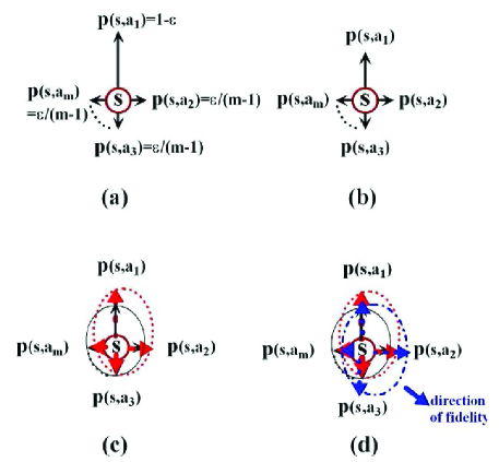
Figure 1: Illustration of the idea of probabilistic action selection method and the effect of fidelity. (a) $\epsilon$-greedy method; (b) Softmax method; (c) basic probabilistic action selection method; (d) fidelity-based probabilistic action selection method.

To sum up, these existing exploration strategies usually suffer from difficulties in balancing between exploration and exploitation, setting appropriate parameters and providing an effective mechanism of re-exploration. Here, we present a novel fidelity-based probabilistic Q-learning algorithm where a probabilistic action selection method is used as more effective exploration strategies to improve the performance of Q-learning for complex learning control problems. Compared with $\epsilon$-greedy and Softmax methods, Fig. 1 shows the illustration of the ideas of straightforward probabilistic action selection method and the fidelity-based one, where a longer line with an arrow indicates a higher probability. As shown in Fig. 1(a), $\epsilon$-greedy method uses a prefixed exploration policy and the action $a_{1}$ with the maximum of Q-value ($Q(s,a_{1})$) is selected with the probability of $(1-\epsilon)$ and all the other actions ($a_{2}\sim a_{m}$) are select with the probability of $\epsilon/(m-1)$, respectively. Using Softmax method (Fig. 1(b)), the action $a_{i},i=1,2,\ldots,m$, is selected with the probability of $\frac{e^{Q(s,a_{i})/\tau}}{\sum_{j=1}^{m}e^{Q(s,a_{j})/\tau}}$. Fig. 1(c) shows that the action selection probability distribution is dynamically updated (denoted with the dashed line) along with the learning process instead of being computed from the estimated Q-values and a temperature parameter. In Fig. 1(d), the fidelity is used to direct the probability distribution and to strengthen the learning effects with a regulation on the updating process. These different exploration policies will be further explained and compared from a point of view of physical mechanism (as shown in Fig. 4) after the PQL and FPQL method are systematically presented in the next section.

III Fidelity-based Probabilistic Q-learning

III-A Probabilistic Action Selection and Reinforcement Strategy

Inspired by the work in [18], [20], we reformulate the action selection strategy in a unified probabilistic representation where the action selection probability distribution is updated based on the reinforcement strategy. The discrete probability distribution on the state-action space is defined as follows.

Definition 1

The probability distribution on the state-action space (discrete case) of a RL problem is characterized by a probability mass function defined on the state set $S$ and the action set $A=\bigcup_{s\in S}A_{(s)}$, where $A_{(s)}$ is the set of all the permitted actions for state $s$. For any $s\in S$ and $a\in A_{(s)}$, the probability mass function is defined as $p(s,a)\geq 0$ and for a certain state $s$, it satisfies

$$\sum_{a\in A_{(s)}}p(s,a)=1.$$ (4)

Suppose the state-action space is $S\times A$, where

$$S=\{s_{1},s_{2},\ldots,s_{n}\}$$ (5)

$$A=\bigcup_{s\in S}A_{(s)}=\{a_{1},a_{2},\ldots,a_{m}\}.$$ (6)

From Definition 1, the policy to be learned $\pi:S\times A\to[0,1]$ can be represented using the probability distribution of the state-action space

$$\pi:P^{\pi}=(p^{\pi}(s,a))_{n\times m}$$ (7)

where $s\in S,a\in A$ and for a certain state $s$, the probability distribution on the action set $A$ is $p_{s}^{\pi}=\{p^{\pi}(s,a_{i})\},i=1,2,\ldots,m$. The look-up table for the Q-values and the probability distribution are of the form

$$\left(\begin{array}[]{ccccc}&\mathbf{a_{1}}&\mathbf{a_{2}}&\cdots&\mathbf{a_{m}}\\ \mathbf{s_{1}}&\left[\begin{split}Q_{(s_{1},a_{1})}\\ p^{\pi}_{(s_{1},a_{1})}\end{split}\right]&\left[\begin{split}Q_{(s_{1},a_{2})}\\ p^{\pi}_{(s_{1},a_{2})}\end{split}\right]&\cdots&\left[\begin{split}Q_{(s_{1},a_{m})}\\ p^{\pi}_{(s_{1},a_{m})}\end{split}\right]\\ \mathbf{s_{2}}&\left[\begin{split}Q_{(s_{2},a_{1})}\\ p^{\pi}_{(s_{2},a_{1})}\end{split}\right]&\ddots&&\vdots\\ \vdots&\vdots&&\ddots&\vdots\\ \mathbf{s_{n}}&\left[\begin{split}Q_{(s_{n},a_{1})}\\ p^{\pi}_{(s_{n},a_{1})}\end{split}\right]&\cdots&\cdots&\left[\begin{split}Q_{(s_{n},a_{m})}\\ p^{\pi}_{(s_{n},a_{m})}\end{split}\right]\\ \end{array}\right).$$ (8)

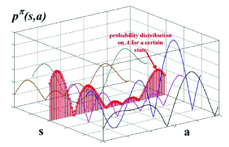
Figure 2: 3-D illustration of probabilistic distribution on the state-action space for action selection under current policy $\pi$.

Fig. 2 shows a 3-D illustration of the probabilistic distribution on the state-action space for action selection under current policy $\pi$. In the probabilistic action selection method, one selects an action $a$ (under policy $\pi$) at a certain state $s$ with the probability according to the probability distribution on the action set $A$, i.e.,

$$a_{s}^{\pi}=f^{\pi}(s)=\begin{cases}a_{1}&\text{with probability}\ p^{\pi}(s,a_{1})\\ a_{2}&\text{with probability}\ p^{\pi}(s,a_{2})\\ \vdots&\\ a_{m}&\text{with probability}\ p^{\pi}(s,a_{m})\\ \end{cases}$$ (9)

Such a probabilistic action selection method leads to a natural probabilistic exploration strategy for Q-learning.

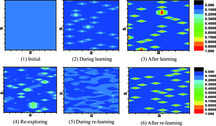
Figure 3: Illustration of the evolution of the probabilistic distribution for action selection on the state-action space during the learning and re-exploring process.

The goal of PQL is to learn a mapping from states to actions. The agent needs to learn a policy $\pi$ to maximize the expected sum of discounted reward for each state:

$$Q_{(s,a)}^{\pi}=\sum_{a\in A_{(s)}}p^{\pi}(s,a)[r_{s}^{a}+\gamma\sum_{s^{\prime}}p_{ss^{\prime}}^{a}Q_{(s^{\prime},a^{\prime})}^{\pi}].$$ (10)

The one-step updating rule of PQL for $Q_{(s,a)}$ is the same as that of QL

$$\small Q(s_{t},a_{t})\leftarrow(1-\alpha_{t})Q(s_{t},a_{t})+\alpha_{t}(r_{t+1}+\gamma\max_{a^{\prime}}Q(s_{t+1},a^{\prime})).$$ (11)

Besides the updating of $Q_{(s,a)}$, the probability distribution is also updated for each learning step. After the execution of action $a_{t}$ for state $s=s_{t}$, the corresponding probability $p(s_{t},a_{t})$ is updated according to the immediate reward $r_{t+1}$ and the estimated value of $Q_{(s^{\prime},a^{\prime})}$ for next state $s^{\prime}=s_{t+1}$

$$p(s_{t},a_{t})\leftarrow p(s_{t},a_{t})+k(r_{t+1}+\max_{a^{\prime}}Q(s_{t+1},a^{\prime})),$$ (12)

where $k$ ($k\geq 0$) is an updating step size and the probability distribution of actions at state $s=s_{t}$ {${p(s,a_{1}),p(s,a_{2}),...,p(s,a_{m})}$} is normalized after each updating. The parameter setting of $k$ is accomplished by experience and generally can be set as the same as the learning rate $\alpha_{t}$. The variation of $k$ in a relatively large range will only slightly affect the learning process because the probability distribution {${p(s,a_{1}),p(s,a_{2}),...,p(s,a_{m})}$} is normalized after each updating step. In particular, $k$ is set as $0.01$ for all the experiments in this paper.

The evolution of the probability distribution of action selection on the state-action space during the whole learning process is shown as in Fig. 3, where the values of the action selection probabilities are represented with different colors. The probability distribution usually starts with an initial uniform one before learning (as shown in Fig. 3(1)), i.e., for each state $s$ the probability distribution of action selection is initialized as $\{p(s,a_{i})=\frac{1}{m},i=1,2,\ldots,m\}$. It evolves with the learning and probability updating process (a sample of the probability distribution during the learning process is shown in Fig. 3(2)) and reaches an optimal one when the learning process ends (Fig. 3(3)). Then the learned policy is applied to the agent (or a control system) and at the same time the learning system may still keep on-line learning capability. If the environment changes the probability distribution will be updated accordingly (Fig. 3(4)) and naturally trigger a re-learning process for the learning system. Fig. 3(5) and Fig. 3(6) show the process of re-learning for a new environment. The characteristics of the proposed probabilistic exploration strategy (as shown in Fig. 3) is very different from the traditional one, e.g., the $\epsilon$-greedy method for Q-learning, where action probability distribution for a certain state keeps constant as shown in Fig. 1(a).

Remark 1

The tradeoff between exploration and exploitation is a specific challenge of RL. Compared with existing exploration strategies, such as $\epsilon$-greedy, Softmax and simulated annealing methods, the probabilistic exploration strategy has the following merits. (i) The learning algorithm possesses more reasonable credit assignment using a probabilistic method and the action selection method is more natural without too much difficulty for parameter setting. The only parameter to be set is the step size $k$. The parameter $k$ will not substantially affect the algorithm performance, because the action selection probabilities for a certain state are relative and will be normalized after each updating step. (ii) The method provides a natural re-exploring mechanism (as shown in Fig. 3), i.e., when the environment changes, the policy also changes along with the on-line learning process. Such a re-exploring mechanism is difficult to implement for the existing exploration strategies (e.g., $\epsilon$-greedy). For example, the value of $\epsilon$ is usually decreased along with the learning process to exploit more after a lot of trials. When the environment changes the value of $\epsilon$ should be reset to avoid too much exploitation. However, it is difficult to do so intelligently. Our scheme provides a straightforward and natural approach for re-exploring mechanism. Although it may need a little bit more physical memories for probability distribution updating, it will not substantially degrade the algorithm, while the performance improvement is more prominent.

III-B Probabilistic Q-learning Algorithms

The procedural form of a probabilistic Q-learning algorithm is presented as Algorithm 1. In this PQL algorithm, after initializing the state and action we can choose $a_{t}$ according to the action probability distribution at state $s_{t}=s$. Execute this action and the system can give the next state $s_{t+1}=s^{\prime}$, immediate reward $r_{t+1}$ and the estimated next state-action function value $Q(s_{t+1},a^{\prime})$. $Q(s_{t},a_{t})$ is updated by the one-step Q-learning rule. The updating of $p(s_{t},a_{t})$ (the probability of choosing $a_{t}$ at state $s_{t}$) is also carried out based on $r_{t+1}$ and $Q(s_{t+1},a^{\prime})$. Hence, in the PQL algorithm, the exploration policy is accomplished through a probability distribution over the action set for each state. When the agent chooses an action at a certain state $s$, the action $a_{i}$ will be selected with probability $p(s,a_{i})$ which is also updated along with the value function updating.

Algorithm 1 Probabilistic Q-learning

1:Initialize $Q(s,a)$ arbitrarily

2:Initialize the policy $\pi:P^{\pi}=(p^{\pi}(s,a))_{n\times m}$ to be evaluated

3:repeat (for each episode)

4:    Initialize $t=1$, $s_{t}$,

5:    repeat (for each step of episode)

6:         $a_{t}\leftarrow$ action $a_{i}$ with probability $p(s_{t},a_{i})$ for $s_{t}$

7:         Take action $a_{t}$, observe reward $r_{t+1}$, and next state $s_{t+1}$

8:         $Q(s_{t},a_{t})\leftarrow Q(s_{t},a_{t})+\alpha_{t}\delta^{Q}_{t+1}$

9:         where $\delta^{Q}_{t+1}=r_{t+1}+\gamma max_{a^{\prime}}Q(s_{t+1},a^{\prime})-Q(s_{t},a_{t})$

10:         $p(s_{t},a_{t})\leftarrow p(s_{t},a_{t})+k(r_{t+1}+max_{a^{\prime}}Q(s_{t+1},a^{\prime}))$

11:         Normalize $\{p(s_{t},a_{i})|_{i=1,2,\ldots,m}\}$

12:         $t\leftarrow t+1$

13:    until  $s_{t+1}$ is terminal

14:until  the learning process ends

Compared with basic Q-learning algorithms, the main feature of the PQL algorithm is the straightforward probabilistic exploration strategy and the reinforcement strategy is also applied to dynamically update the probability distribution of action selection. The agent selects actions based on the variable probability distribution over an admissible action set at a certain state. Such an action selection method keeps a proper chance of exploration instead of obeying the policy learned so far, and makes a good tradeoff between exploration and exploitation using probability.

III-C Fidelity-based PQL Algorithm

PQL uses a probabilistic action selection method to improve the exploration strategy and is an effective approach for stochastic learning and optimization. But for most complex reinforcement learning problems, the direction of achieving the objective is always delayed due to the lack of feedback information during the learning process unless the agent reaches the target state. Hence, if we can extract more information from the system structure or system behavior, the learning performance can be further improved for complex learning problems with large learning space. Because most of quantum control problems are complex and the concept of fidelity is widely used in quantum information community [19], [39], [40], we develop a fidelity-based PQL method for learning control of quantum systems, which can also be applied to some other complex RL problems.

The updating rule of fidelity-based PQL for $Q_{(s,a)}$ is the same as (11). The probability distribution is updated for each learning step. After the execution of action $a_{t}$ for state $s=s_{t}$, the corresponding probability $p(s_{t},a_{t})$ is updated according to the immediate reward $r_{t+1}$, the estimated value of $Q_{(s_{t+1},a^{\prime})}$ for next state $s^{\prime}=s_{t+1}$ and the fidelity $F(s_{t+1},s_{\text{target}})$ between the state $s_{t+1}$ and the target state $s_{\text{target}}$. That is

$$\small p(s_{t},a_{t})\leftarrow p(s_{t},a_{t})+k(r_{t+1}+\max_{a^{\prime}}Q(s_{t+1},a^{\prime})+F(s_{t+1},s_{\text{target}})).$$ (13)

The specification of the fidelity $F(s_{t+1},s_{\text{target}})$ is defined regarding the objective of the learning control task. In this study, a fidelity of quantum pure states (see Subsection IV-A) is adopted for the learning control of quantum systems. The parameter setting methods and the normalization of the probability distribution of actions at state $s=s_{t}$ are the same as that of PQL. The procedure of the fidelity-based PQL algorithm is shown as Algorithm 2.

Algorithm 2 Fidelity-based Probabilistic Q-learning

1:Initialize $Q(s,a)$ arbitrarily

2:Initialize the policy $\pi:P^{\pi}=(p^{\pi}(s,a))_{n\times m}$ to be evaluated

3:repeat (for each episode)

4:    Initialize $t=1$, $s_{t}$

5:    repeat (for each step of episode)

6:         $a_{t}\leftarrow$ action $a_{i}$ with probability $p(s_{t},a_{i})$ for $s_{t}$

7:         Take action $a_{t}$, observe reward $r_{t+1}$, and next state $s_{t+1}$

8:         $Q(s_{t},a_{t})\leftarrow Q(s_{t},a_{t})+\alpha_{t}\delta^{Q}_{t+1}$

9:         where $\delta^{Q}_{t+1}=r_{t+1}+\gamma max_{a^{\prime}}Q(s_{t+1},a^{\prime})-Q(s_{t},a_{t})$

10:         $p(s_{t},a_{t})\leftarrow p(s_{t},a_{t})+k\delta^{p}_{t+1}$

11:         where $\delta^{p}_{t+1}=r_{t+1}+max_{a^{\prime}}Q(s_{t+1},a^{\prime})+F(s_{t+1},s_{\text{target}})$

12:         Normalize $\{p(s_{t},a_{i})|_{i=1,2,\ldots,m}\}$

13:         $t\leftarrow t+1$

14:    until  $s_{t+1}$ is terminal

15:until  the learning process ends

As for the convergence of FPQL, it is the same as that of basic Q-learning [3], because the difference only lies in the exploration policy which does not affect the convergence of the algorithms. Several constraints [3], [43] are listed in Theorem 1 to ensure the convergence of FPQL.

Theorem 1 (Convergence of FPQL)

Consider an FPQL agent in a nondeterministic Markov decision process, for every state-action pair $s$ and $a$, the Q-value $Q_{t}(s,a)$ will converge to the optimal state-action value function $Q^{*}(s,a)$ if the following constraints are satisfied

1. The rewards in the whole learning process satisfy $(\forall s,a)|r_{s}^{a}|\leq R$, where $R$ is a finite constant value;

2. A discount factor $\gamma\in[0,1)$ is adopted;

3. During the learning process, the nonnegative learning rate $\alpha_{t}$ satisfies

   $$\lim_{T\to\infty}\sum_{t=1}^{T}\alpha_{t}=\infty,\ \ \ \ \lim_{T\to\infty}\sum_{t=1}^{T}\alpha_{t}^{2}<\infty.$$ (14)

The difference between the proposed fidelity-based probabilistic exploration strategy and the existing exploration strategies can be explained from a point of view of physical mechanism. As shown in Fig. 4, for a learning optimization problem, the existing exploration strategies, e.g., $\epsilon$-greedy, softmax and simulated annealing methods, apply a thermal fluctuation type of exploration methods to acquire the chance of stepping over the local optima; while the probabilistic exploration strategy is inspired by quantum phenomena. It behaves like quantum tunnelling effect and can step over the local optima in a more straightforward way. The direction of the fidelity can strength this tunnelling effect. The physical explanation can help demonstrate why the fidelity-based probabilistic method may perform better for complex reinforcement learning tasks.

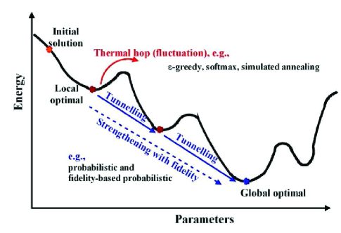
Figure 4: A schematic of physical explanation and comparison of different exploration strategies for optimization and learning methods.

Remark 2

Although the fidelity-based PQL method is proposed for learning control of quantum systems, it can also be applied to other RL problems when there is a clear and quantitative definition of fidelity that can effectively characterize the distance between the current state and the target state. The fidelity information can speed up the learning process in that it shows the direction to the target state and can help the learning process get out of the traps when get lost. In addition, this fidelity signal is only used to regulate the action selection probability distribution. It will not deteriorate the exploration strategy of PQL.

Remark 3

It is clear that the optimal policy of FPQL is closely related to the probability distribution of the actions for each state, which means the learning process essentially is also the process of reducing the uncertainty of decisions on which action should be chosen at a state. Hence, the characteristics of the FPQL algorithm and its performance can also be described with the degree of uncertainty for action selection. The measurement of uncertainty has been well addressed through Shannon entropy (i.e., Shannon measure of uncertainty) [44] in information science, where the amount of uncertainty is measured by a probability distribution function $p$ on a finite set: $S(p)=-\sum_{x\in X}p(x)\log_{2}p(x)$, where $X$ is the universal set, $x$ is the element of the finite set $X$ and $p(x)$ is the probability distribution function on $X$. Similar to Shannon entropy, the concept of Exploration Entropy can also be given based on the probability distributions of actions to measure the uncertainty of action selection. The resulting function is $E_{(s)}=-\sum P_{(a_{i}|s)}\log_{2}P_{(a_{i}|s)}$. For an FPQL system, the general uncertainty of action selection can be described with the mean exploration entropy $\overline{E_{(s)}}=\frac{\sum_{j=1,2,...,n}E_{(s_{j})}}{n}$, where $S=\{s_{1},s_{2},...,s_{n}\}$ is the state set. It is clear that when all the probabilities are equal the exploration entropy (uncertainty of action selection) will be maximum. In an FPQL system, the maximum exploration entropy of a state $s$ with $m$ actions will be $\log_{2}m$. The maximum mean decision entropy $\overline{E_{(s)}}$ should be obtained when all the action probability distributions for each state are uniform, which is always the situation at the initialization without any prior knowledge about the environment. Along with the learning process, $\overline{E_{(s)}}$ will tend to decrease and obtain its minimum when the learning process converges and gives the optimal policy.

IV Fidelity-based PQL for learning control of quantum systems

IV-A Learning control of quantum systems

Learning control is an effective method for quantum systems where a control law can be learned from experience and the system performance can be optimized by searching for an optimal control strategy in an iterative way [21], [45]-[47]. Here, we focus on the control problem of quantum pure state transition for $N$-level quantum systems [38]. Denote the eigenstates of the free Hamiltonian $H_{0}$ of an $N$-level quantum system as $D=\{|\phi_{i}\rangle\}_{i=1}^{N}$. An evolving state $|\psi(t)\rangle$ of the controlled system can be expanded in terms of the eigenstates in the set $D$:

$$|\psi(t)\rangle=\sum_{i=1}^{N}c_{i}(t)|\phi_{i}\rangle$$ (15)

where complex numbers $c_{i}(t)$ satisfy $\sum_{i=1}^{N}|c_{i}(t)|^{2}=1$. We have the definition of fidelity between two pure states.

Definition 2 (Fidelity of Quantum Pure States)

The fidelity between two pure states $|\psi^{a}\rangle=\sum_{i=1}^{N}c^{a}_{i}|\phi_{i}\rangle$ and $|\psi^{b}\rangle=\sum_{i=1}^{N}c^{b}_{i}|\phi_{i}\rangle$ is defined as

$$F(|\psi^{a}\rangle,|\psi^{b}\rangle)=|\langle\psi^{a}|\psi^{b}\rangle|=|\sum^{N}_{i=1}(c^{a}_{i})^{*}c^{b}_{i}|,$$ (16)

where $(c^{a}_{i})^{*}$ is the complex conjugate of $c^{a}_{i}$.

Introducing a control $\varepsilon(t)\in L^{2}(\mathbf{R})$ acting on the system via a time-independent interaction Hamiltonian $H_{I}$ and denoting $|\psi(t=0)\rangle$ as $|\psi_{0}\rangle$, $C(t)=(c_{i}(t))_{i=1}^{N}$ evolves according to the Schrödinger equation [32]:

$$\left\{\begin{split}&\iota\hbar\dot{C}(t)=[A+\varepsilon(t)B]C(t)\\ &C(t=0)=C_{0}\end{split}\right.$$ (17)

where $\iota=\sqrt{-1}$, $C_{0}=(c_{0i})_{i=1}^{N}$, $c_{0i}=\langle\phi_{i}|\psi_{0}\rangle$, $\sum_{i=1}^{N}|c_{0i}|^{2}=1$, $\hbar$ is the reduced Planck constant, and the matrices $A$ and $B$ correspond to $H_{0}$ and $H_{I}$, respectively. We assume that the $A$ matrix is diagonal and the $B$ matrix is Hermitian [32]. In order to avoid trivial control problems we assume $[A,B]\equiv AB-BA\neq 0$. Equation (17) describes the evolution of a finite dimensional control system. The propagator $U(t_{1}\rightarrow t_{2})$ is a unitary operator such that for any state $|\psi(t_{1})\rangle$ the state $|\psi(t_{2})\rangle=U(t_{1}\rightarrow t_{2})|\psi(t_{1})\rangle$ is the solution at time $t=t_{2}$ of (15) and (17) with the initial condition $|\psi(t_{1})\rangle$ at time $t=t_{1}$. $U(t_{1}\rightarrow t_{2})$ is also simplified as $U(t)$, $t\in[t_{1},t_{2}]$, if the specific time $t_{1}$ can be neglected when handling these problems. Assume that the control set $\{\varepsilon_{j},j=1,\dots,m\}$ is given. Every control $\varepsilon_{j}$ corresponds to a unitary operator $U_{j}$. The task of learning control is to find a control sequence $\{\varepsilon_{l},l=1,2,3,\dots\}$ where $\varepsilon_{l}\in\{\varepsilon_{j},j=1,\dots,m\}$ to drive the quantum system from an initial state $|\psi_{0}\rangle$ to the target state $|\psi_{f}\rangle$.

Remark 4

In the past decade, the research areas of quantum information and machine learning have mutually benefitted from each other. On one hand, quantum characteristics have been used for designing quantum or quantum-inspired learning algorithms [18], [19], [48]-[52]. On the other hand, many traditional learning algorithms have been applied for the control design of quantum phenomena, including gradient-based algorithms [42], [53], genetic algorithm (GA) [45], [54] and fuzzy logic [38]. For example, gradient-based methods have been widely used in model-based control design and theoretical analysis of quantum systems. Since we assume that very limited control resources are available, gradient-based algorithms cannot be applied to the quantum control problem in this paper. GA methods have achieved great success for quantum learning control in laboratory [45]. However, a large amount of experimental data is required to optimize the control performance since the closed-loop learning process involves the collection of experimental data and the searching of optimized pulses based on the updating of experimental data [45]. In this paper, we consider a class of quantum control problems with a limited set of control fields. This class of problems is significant in quantum control since different constraints are common for quantum control systems. We formulate this class of quantum control problems as a model-free sequential Markovian decision process (MDP). Reinforcement learning is a good candidate to solve a MDP problem. Hence, we apply the proposed FPQL approach to this class of quantum control problems that can be used to test the effectiveness of FPQL as well as to provide an effective design approach for quantum systems with limited control resources.

IV-B Quantum controlled transition landscapes

Learning control of quantum systems aims to find an optimal control strategy to manipulate the dynamics of physical processes on the atomic and molecular scales [45]. In recent years, quantum control landscapes [41], [42] provide a theoretical footing for analyzing learning control of quantum systems. A control landscape is defined as the map between the time-dependent control Hamiltonian and associated values of the control performance functional. Most quantum control problems can be formulated as the maximization of an objective performance function. For example, as shown in Fig. 5, the performance function $J(\varepsilon)$ is defined as the functional of the control strategy $\varepsilon={\varepsilon_{i},i=1,2,...,M}$, where $M$ is a positive integer that indicates the number of the control variables ($M=2$ for the case shown in Fig. 5).

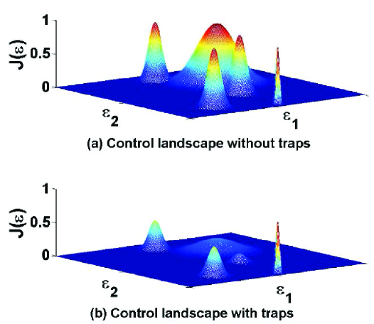
Figure 5: An example of quantum control landscapes. (a) Quantum control landscape without traps (local maxima) where all the peaks are of the same height and thus all of them are global maxima; (b) Quantum control landscape with traps where the landscape has one highest peak representing the global maximum and several peaks of lower height corresponding to local maxima.

Although quantum control applications may span a variety of objectives, most of them correspond to maximizing the probability of transition from an initial state $|\psi_{0}\rangle$ to a desired final state $|\psi_{f}\rangle$ [41]. For the state transition problem with $t\in[0,T]$, we define the quantum controlled transition landscape as

$$J(\varepsilon)=\text{tr}(U_{(\varepsilon,T)}|\psi_{0}\rangle\langle\psi_{0}|U^{{\dagger}}_{(\varepsilon,T)}|\psi_{f}\rangle\langle\psi_{f}|),$$ (18)

where $\text{tr}(\cdot)$ is the trace operator and $U^{{\dagger}}$ is the adjoint of $U$. The objective of the learning control system is to find a global optimal control strategy $\varepsilon^{*}$ which satisfies

$$\varepsilon^{*}=\text{argmax}_{\varepsilon}J(\varepsilon).$$ (19)

If the dependence of $U_{(T)}$ on $\varepsilon$ is suppressed (see [42]), (18) can be reformulated as

$$J(U)=\text{tr}(U_{(T)}|\psi_{0}\rangle\langle\psi_{0}|U^{{\dagger}}_{(T)}|\psi_{f}\rangle\langle\psi_{f}|).$$ (20)

Equations (18) and (20) are called the dynamic control landscape (denoted as $J_{D}(\varepsilon)$ instead) and the kinematic landscape (denoted as $J_{K}(U)$ instead), respectively (see [42]).

The characteristic of the existence or absence of traps is most important for exploring the quantum control landscape with a learning control algorithm, which can be studied using critical points. A dynamic critical point is defined by

$$\nabla J_{D}(\varepsilon)=\delta J_{D}(\varepsilon)/\delta\varepsilon=0$$ (21)

and a kinematic critical point is defined by

$$\nabla J_{K}(U)=\delta J_{K}(U)/\delta U=0$$ (22)

where $\nabla$ denotes gradient. By the chain rule, we have

$$\nabla J_{D}(\varepsilon)=\frac{\delta J_{K}(U)}{\delta U_{(\varepsilon,T)}}\frac{\delta U_{(\varepsilon,T)}}{\delta\varepsilon}=\nabla J_{K}(U)\frac{\delta U_{(\varepsilon,T)}}{\delta\varepsilon}.$$ (23)

According to the results in [42], we can summarize the properties of quantum controlled transition landscape as Theorem 2.

Theorem 2

For the quantum control problem defined with the dynamic control landscape (18) and the kinematic control landscape (20), respectively, the properties of the solution sets of the quantum controlled transition landscape are listed as follows:

1. The kinematic control landscape is free of traps (i.e., all critical points of $J_{K}(U)$ are either global maxima or saddles) if the operator $U$ can be any unitary operator (i.e., the system is completely controllable);

2. The dynamic control landscape is free of traps if (i) the operator $U$ can be any unitary operator and (ii) the Jacobian $\delta U_{(\varepsilon,T)}/\delta\varepsilon$ has full rank at any $\varepsilon$.

For detailed proof and discussion about Theorem 2, please refer to [41], [42].

Remark 5

The quantum controlled transition landscape theory is the theoretical foundation for learning control design. The FPQL algorithm has potential for quantum learning control problems. The reasons can be stated from three aspects: (i) The probabilistic action selection method makes a better balance between exploration and exploitation, since too much exploitation is easy to be trapped and too much exploration will deteriorate the learning performance; (ii) The theoretical analysis of the solution sets of a quantum control landscape can help design a fidelity-based method to improve the learning performance; (iii) The learning scheme of reinforcement learning is more suitable for model-free real laboratory applications than typical gradient-based methods which need specific models.

In the next two subsections, the learning control problems of a spin-$\frac{1}{2}$ system and a $\Lambda$-type atomic system are studied using the proposed FPQL algorithm, which shows that FPQL is an alternative effective approach for quantum control design.

IV-C Example 1: learning control of a spin-$\frac{1}{2}$ quantum system

The spin-$\frac{1}{2}$ system is a typical 2-level quantum system and has important theoretical implications and practical applications. Its Bloch vector can be visualized on a 3D Bloch sphere as shown in Fig. 6. The state of the spin-$\frac{1}{2}$ quantum system $|\psi\rangle$ can be represented as

$$|\psi\rangle=\cos\frac{\theta}{2}|0\rangle+e^{i\varphi}\sin\frac{\theta}{2}|1\rangle$$ (24)

where $\theta\in[0,\pi]$ and $\varphi\in[0,2\pi]$ are polar angle and azimuthal angle, respectively, which specify a point $\overrightarrow{a}=(x,y,z)=(\sin\theta\cos\varphi,\sin\theta\sin\varphi,\cos\theta)$ on the unit sphere in $\mathbf{R}^{3}$.

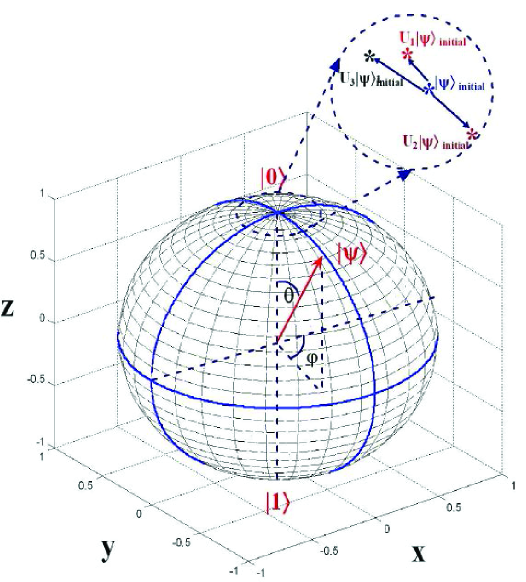
Figure 6: Demonstration of a spin-$\frac{1}{2}$ system with a Bloch sphere in a 3D Cartesian coordinates and the state transitions for an initial quantum state $|\psi\rangle_{initial}$ using different one-step controls ($U_{1}$,$U_{2}$,$U_{3}$)

At each control step, the permitted controls for every state are $U_{1}$ (no control input), $U_{2}$ (a positive pulse control) and $U_{3}$ (a negative pulse control). Fig. 6 shows a sketch map of one-step control effects on the evolution of the quantum system. The propagators $\{U_{i},i=1,2,3\}$ are listed as follow:

$$U_{1}=e^{-iI_{z}\frac{\pi}{15}},$$ (25)

$$U_{2}=e^{-i(I_{z}+0.5I_{x})\frac{\pi}{15}},$$ (26)

$$U_{3}=e^{-i(I_{z}-0.5I_{x})\frac{\pi}{15}},$$ (27)

where

$$I_{z}=\frac{1}{2}\begin{pmatrix}1&0\\ 0&-1\\ \end{pmatrix},\ \ I_{x}=\frac{1}{2}\begin{pmatrix}0&1\\ 1&0\\ \end{pmatrix}.$$ (28)

Figure 7: Demonstration of a stochastic control case without learning. The left figure shows the state transition path and the right figure shows the control sequence used (0 for no pulse, -1 for negative pulse and +1 for positive pulse)

Now the control objective is to control the spin-$\frac{1}{2}$ system from the initial state $(\theta=\frac{\pi}{60},\varphi=\frac{\pi}{30})$ to the target state $(\theta=\frac{41\pi}{60},\varphi=\frac{29\pi}{30})$ with minimized control steps. Fig. 7 shows one of the control process before learning, where the controls are selected randomly and after a long control sequence the system state may be transited to the target state. We apply the fidelity-based PQL, PQL and QL algorithms to this learning control problem, respectively. Now we reformulate the RL problem of controlling a quantum system from an initial state $s_{\text{initial}}=|\psi_{\text{initial}}\rangle$ to a desired target state $s_{\text{target}}=|\psi_{\text{target}}\rangle$ as follows: the state set is $S=\{s_{i}=|\psi_{\text{i}}\rangle\},i=1,2,\ldots,n$ and the action set is $A=\{a_{j}=u_{j}\},j=1,2,\ldots,m$. The experiment settings for these algorithms are listed as follows: $r=-1$ for each control step until it reaches the target state, then it gets a reward of $r=1000$; the discount factor $\gamma=0.99$, the learning rate $\alpha=0.01$ and the Q-values are all initialized as 0. For PQL and fidelity-based PQL, $k=0.01$. The $\epsilon$-greedy exploration strategy is used and $\epsilon=0.1$.

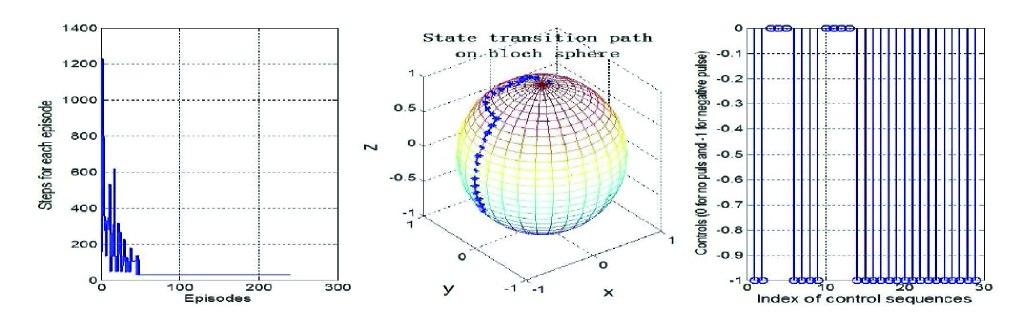
Figure 8: Learning performance of fidelity-based PQL and the learning results with an optimal control sequence

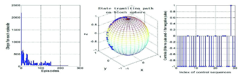
Figure 9: Learning performance of PQL and the learning results with an optimal control sequence

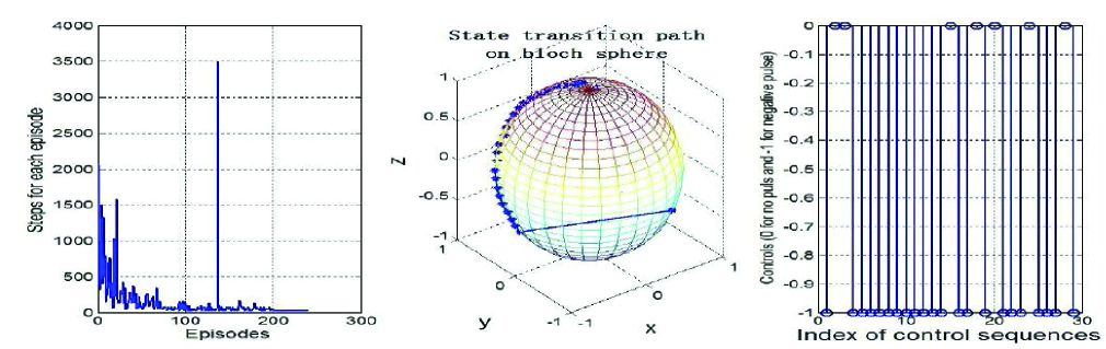
Figure 10: Learning performance of standard QL with $\varepsilon$-greedy policy and the learning results with an optimal control sequence

Figs. 8-10 show the control performance of all these algorithms, respectively. Hundreds of times of learning process are carried out for each experiment and all the results maintain similar performance. We provide the results of one time of learning process for each experiment. The experimental results show that fidelity-based PQL outperforms PQL and standard QL. The fidelity-based PQL quickly find the optimal control sequence after less than 50 episodes, while PQL needs about 150 episodes and QL needs more than 200 episodes. For each episode in the learning process, QL and PQL also need much more steps to find the target state. A clearer performance comparison between the fidelity-based PQL, PQL and QL is shown as in Fig. 11. It is clear that the fidelity-based method contributes to more effective tradeoff between exploration and exploitation than PQL and confines it from exploring too much in an economical way with respect to exploration cost. Although the fidelity-based PQL needs a little more steps in the early learning stage (which makes its performance lies between QL and PQL), it can quickly converge to the optimal policy and remarkably outperforms both of QL and PQL. The final control results with the learned optimal control sequence that controls the spin-$\frac{1}{2}$ quantum state from the initial state to the target state is demonstrated in Fig. 12.

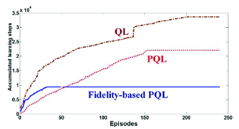
Figure 11: Comparison of Learning performances between Fidelity-based PQL, PQL and QL

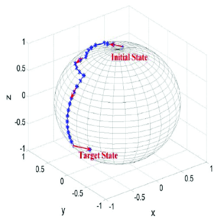
Figure 12: The control results with the learned optimal control sequence

IV-D Example 2: learning control of a $\Lambda$-type quantum system

Now we consider a $\Lambda$-type atomic system and demonstrate the fidelity-based PQL design process. The three level $\Lambda$-type atomic system is a representative of the multi-level system, which has wide applications in the fields of chemistry, quantum physics and quantum information [55]. For the $\Lambda$-type system shown in Fig. 13, the evolving state $|\psi(t)\rangle$ can be expanded in terms of the eigenstates as follows:

Figure 13: A schematic of a 3-level $\Lambda$-type atomic system.

$$|\psi(t)\rangle=c_{1}(t)|1\rangle+c_{2}(t)|2\rangle+c_{3}(t)|3\rangle,$$ (29)

where $|1\rangle$, $|2\rangle$ and $|3\rangle$ are the basis states of the lower, middle and upper atomic states, respectively. At each control step, the permitted controls are a finite number of (positive or negative) control pulses, i.e., we have the propagators

$$U_{E}=e^{-i\Delta t(H_{0}+0.1EH_{1})}$$ (30)

where $\Delta t=0.1$,

$$\small H_{0}=\left(\begin{array}[]{ccc}1.5&0&0\\ 0&1&0\\ 0&0&0\\ \end{array}\right),\ H_{1}=\left(\begin{array}[]{ccc}0&0&1\\ 0&0&1\\ 1&1&0\\ \end{array}\right),$$ (31)

and $E\in\{0,\pm 1,\pm 2,\ldots,\pm 20\}$ is the number of chosen control pulses at a certain control step.

Now the control objective is to control the $\Lambda$-type atomic system from the initial state $|\psi_{\text{initial}}\rangle=(1,0,0)$ to the target state $|\psi_{\text{target}}\rangle=(0,0,1)$ with a fixed number of control steps. We apply the fidelity-based PQL, PQL and QL algorithms to this learning control problem, respectively. First we reformulate the RL problem of controlling a quantum system from an initial state $s_{\text{initial}}=|\psi_{\text{initial}}\rangle$ to a desired target state $s_{\text{target}}=|\psi_{\text{target}}\rangle$ as follows: the number of control steps is fixed as a constant number of $100$, so that we can use a virtual state set to construct the state-action space instead of the real state space (with a very high dimension) of the $\Lambda$-type system and the state set $S=\{s_{i}\},i=1,2,\ldots,101$ and the action set is $A=\{a_{j}=E_{j}=j-21\},j=1,2,\ldots,41$. The experiment settings for these algorithms are listed as follows: $r=0$ for each control step until it reaches the target state at the end of the control process where it gets a reward of $r=1000$; the discount factor $\gamma=0.99$, the learning rate $\alpha=0.01$ and the Q-values are all initialized as 0. For PQL and fidelity-based PQL, $k=0.01$. The $\epsilon$-greedy exploration strategy is used for QL and $\epsilon=0.1$. The fidelity for a current policy $\pi$ is defined as $F=|\langle\psi^{\pi}_{f}|\psi_{\text{target}}\rangle|$.

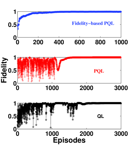
Figure 14: Control performances with respect to the fidelity between the final state and the target state using fidelity-based PQL, PQL and QL, respectively.

The learning performances of fidelity-based PQL, PQL and QL are shown in Fig. 14 with respect to fidelity, which is one of all the alike results for hundreds of experiments we carried out. The learning process converges after about $300$ episodes using fidelity-based PQL, while PQL needs about $1450$ episodes and QL needs about $2000$ episodes. The oscillation for PQL and QL before the learning processes converge in Fig. 14 is due to the performance criteria regarding fidelity instead of accumulated learning steps as used in Fig. 11. The performance shown in Fig. 14 is very sensitive to the exploration behavior in the state-action space for PQL and QL, while the fidelity-based method shows an almost monotonically improved learning behavior.

The final optimal control sequence is shown in Fig. 15. With this learned optimal control sequence the $\Lambda$-type atomic system described by Equations (29)-(31) is controlled from the initial state $|\psi_{\text{initial}}\rangle=(1,0,0)$ to the target state $|\psi_{\text{target}}\rangle=(0,0,1)$ and the population evolution trajectories are demonstrated in Fig. 16. All these numerical results demonstrate the success of the proposed fidelity-based PQL method. In addition, the learning control of the $\Lambda$-type atomic system can also be implemented with policy iteration [9], [10], but it is out of the scope of this paper. More comparison results between the value iteration and policy iteration for reinforcement learning will be presented in our future work.

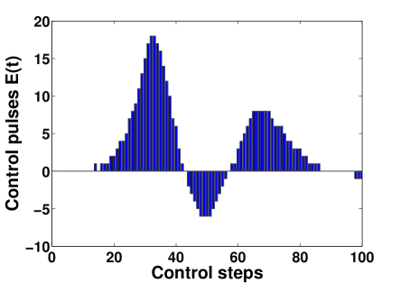
Figure 15: The learned optimal control pulse sequence.

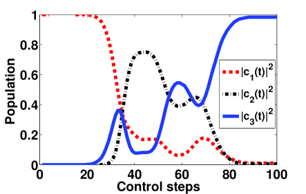
Figure 16: The population evolution trajectories with the learned optimal control pulse sequence.

V Conclusions

In this paper, a probabilistic action selection method is introduced for Q-learning and an FPQL algorithm is presented for the learning control design of quantum systems. In FPQL, the fidelity information can be extracted from the system structure or the system behavior. The aim is to design a good exploration strategy for a better tradeoff between exploration and exploitation and to speed up the learning process as well. The experimental results show that FPQL is superior to basic Q-learning with respect to convergence speed. The control problems of a spin-$\frac{1}{2}$ system and a $\Lambda$-type atomic system are adopted to demonstrate the performance of FPQL. Although all the cases we considered in this study are discrete examples, which are most widely used in practical applications, the proposed fidelity-based probabilistic action selection method can be extended to other reinforcement learning algorithms and applications using function approximation with a continuous probability distribution and related iteration methods. In addition, our future work will focus on further comparison of FPQL with other existing learning methods (e.g., GA, gradient-base methods and neural networks) for more general quantum control problems.

References

- [1] R. Sutton and A. G. Barto, Reinforcement Learning: An Introduction. Cambridge, MA: MIT Press, 1998.
- [2] R. Sutton, “Learning to predict by the methods of temporal difference,” Machine Learning, vol.3, pp.9-44, 1988.
- [3] C. Watkins and P. Dayan, “Q-learning,” Machine Learning, vol.8, pp.279-292, 1992.
- [4] T. Kondo and K. Ito, “A reinforcement learning with evolutionary state recruitment strategy for autonomous mobile robots control,” Robotics and Autonomous Systems, vol.46, pp.111-124, 2004.
- [5] L. Busoniu, R. Babuska and B. De Schutter, “A comprehensive survey of multiagent reinforcement learing,” IEEE Transactions on Systems, Man, and Cybernetics C, vol.38, no.2, pp.156-172, 2008.
- [6] A. H. Tan, N. Lu and D. Xiao, “Integrating temporal difference methods and self-organizing neural networks for reinforcement learing with delay evaluative feedback,” IEEE Transactions on Neural Networks, vol.19, no.2, pp.230-244, 2008.
- [7] F. Y. Wang, H. G. Zhang and D. Liu, “Adaptive dynamic programming: An introduction,” IEEE Computational Intelligence Magazine, vol.4, no.2, pp.39-47, 2009.
- [8] C. W. Anderson, P. M. Young, M. R. Buehner, J. N. Knight, K. A. Bush and D. C. Hittle, “Robust reinforcement leanring control using integral quadratic constraints for recurrent neural networds,” IEEE Transactions on Neural Networks, vol.18, no.4, pp.993-1002, 2007.
- [9] X. Xu, D. Hu and X. Lu, “Kernel-based least squares policy iteration for reinforcement learning,” IEEE Transactions on Neural Networks, vol.18, no.4, pp.973-992, 2007.
- [10] X. Xu, C.M. Liu, S.X. Yang and D.W. Hu, “Hierarchical approximate policy iteration with binary-tree state space decomposition”, IEEE Transactions on Neural Networks, vol.22, no.12, pp.1863-1877, 2011.
- [11] Z. Yang, S.C.P. Yam, L.K. Li and Y. Wang, “Universal repetitive learning control for nonparametric uncertainty and unknown control gain matrix”, IEEE Transactions on Automatic Control, vol.55, no.7, pp.1710-1715, 2010.
- [12] Y. Li, B. Yin and H. Xi, “Finding optimal memoryless policies of POMDPs under the expected average reward criterion”, European Journal of Operational Research, vo.211, no.3, pp.556-567, 2011.
- [13] X.S. Wang, Y.H. Cheng and J.Q. Yi, “A fuzzy actor-critic reinforcement learning network”, Information Sciences, vol.177, pp.3764-3781, 2007.
- [14] H. Zhang, Q. Wei and D. Liu, “An iterative adaptive dynamic programming method for solving a class of nonlinear zero-sum differential games,” Automatica, vol.47, no.1, pp.207-214, 2011.
- [15] D. Wang, D. Liu, Q. Wei, D. Zhao and N. Jin, “Optimal control of unknown nonaffine nonlinear discrete-time systems based on adaptive dynamic programming”, Automatica, vol.48, no.8, pp.1825-1832, 2012.
- [16] D. Dong, C. Chen, J. Chu and T.J. Tarn, “Robust quantum-inspired reinforcement learning for robot navigation”, IEEE/ASME Transactions on Mechatronics, vol.17, pp.86-97, 2012.
- [17] Q. Yang and S. Jagannathan, “Reinforcement learning controller design for affine nonlinear discrete-time systems using online approximators”, IEEE Transactions on Systems, Man and Cybernetics B, vol.42, no.2, pp.377-390, 2012.
- [18] D. Dong, C. Chen, H. Li and T. J. Tarn, “Quantum reinforcement learning,” IEEE Transactions on Systems, Man, and Cybernetics B, vol.38, no.5, pp.1207-1220, 2008.
- [19] M. A. Nielsen and I. L. Chuang, Quantum Computation and Quantum Information. Cambridge, England: Cambridge University Press, 2000.
- [20] C. Chen, D. Dong and Z. Chen, “Quantum computation for action selection using reinforcement learning,” International Journal of Quantum Information, vol.4, no.6, pp.1071-1083, 2006.
- [21] D. Dong, C. Chen, T. J. Tarn, A. Pechen and H. Rabitz, “Incoherent control of quantum systems with wavefunction controllable subspaces via quantum reinforcement learning,” IEEE Transactions on Systems, Man, and Cybernetics B, vol.38, no.4, pp.957-962, 2008.
- [22] C. Chen, P. Yang, X. Zhou and D. Dong, “A quantum-inspired Q-learning algorithm for indoor robot navigation,” in Proceedings of the 2008 IEEE International Conference on Networking, Sensing and Control, pp.1599-1603, IEEE Press, Sanya, China, 2008.
- [23] M. Z. Guo, Y. Liu and J. Malec, “A new Q-learning algorithm based on the metropolis criterion,” IEEE Transactions on Systems, Man, and Cybernetics B, vol.34, no.5, pp.2140-2143, 2004.
- [24] K. Iwata, K. Ikeda and H. Sakai, “A new criterion using information gain for action selection strategy in reinforcement learning,” IEEE Transactions on Neural Networks, vol.15, no.4, pp.792-799, 2004.
- [25] T. Rückstiess, F. Sehnke, T. Schaul, D. Wierstra, S. Yi, J. Schmidhuber, “Exploring parameter space in reinforcement learning,” Paladyn Journal of Behavioral Robotics, vol.1, no.1, pp. 14-24, 2010.
- [26] C. Cai, X. Liao and L. Carin, “Learn to explore and exploit in POMDPs,” in Proceedings of the 23th Conference on Neural Information Processing Systems, pp. 198-206, Vancouver, BC, Canada, Dec. 2009.
- [27] P. Abbeel and A. Y. Ng, “Exploration and apprenticeship learning in reinforcement learning,” in Proceedings of International Conference on Machine Learning, Bonn, Germany, 2005.
- [28] M. Tokic, G. Palm, “Gradient algorithms for exploration/exploitation trade-Offs: global and local variants,” Lecture Notes in Computer Science, Vol. 7477, pp. 60-71, 2012.
- [29] P. Poupart, M. Ghavamzadeh and Y. Engel, Tutorial on Bayesian methods for reinforcement learning, International Conference on Machine Learning, Corvallis, USA, June 20-24, 2007. https://cs.uwaterloo.ca/~ppoupart/ICML-07-tutorial-Bayes-RL.html.
- [30] D Kim, K. E. Kim and P. Poupart, “Cost-sensitive exploration in bayesian reinforcement learning,” in Proceedings of Neural Information Processing Systems, Th21(1-9), Lake Tahoe, Nevada, USA, December 3-8, 2012.
- [31] M. Bowling and M. Veloso, “Rational and convergent learning in stochastic games,” in Proceedings of the Seventeenth International Joint Conference on Artificial Intelligence, pp. 1021-1026, Seattle, Washington, USA, August 2001.
- [32] D. Dong and I.R. Petersen, “Quantum control theory and applications: A survey,” IET Control Theory & Applications, Vol. 4, pp. 2651-2671, 2010.
- [33] H.M. Wiseman and G.J. Milburn, Quantum Measurement and Control, Cambridge, England: Cambridge University Press, 2010.
- [34] D. Dong and I.R. Petersen, “Sliding mode control of two-level quantum systems”, Automatica, vol.48, pp.725-735, 2012.
- [35] C. Altafini and F. Ticozzi, “Modeling and control of quantum systems: an introduction”, IEEE Transactions on Automatic Control, vol. 57, pp.1898-1917, 2012.
- [36] B. Qi, H. Pan and L. Guo, “Futher results on stabilizing control of quantum systems”, IEEE Transactions on Automatic Control, vol. 58, pp.1349-1354, 2013.
- [37] D. Dong, I.R. Petersen and H. Rabitz, “Sampled-data design for robust control of a single qubit”, IEEE Transactions on Automatic Control, vol. 58, pp.2054-2059, 2013.
- [38] C. Chen, D. Dong, J. Lam and T. J Tarn, “Control design of uncertain quantum systems with fuzzy estimators,” IEEE Transactions on Fuzzy Systems, vol.20, no.5, pp.820-831, 2012.
- [39] M. G. Bason, et al, “High-fidelity quantum driving,” Nature Physics, vol. 8, pp.147-152, 2011.
- [40] M. Cozzini, R. Ionicioiu and P. Zanardi, “Quantum fidelity and quantum phase transitions in matrix product states,” Physical Review B, vol. 76, p.104420, 2007.
- [41] H. Rabitz, M. Hsieh and C. Rosenthal, “Quantum optimally controlled transition landscapes,” Science, vol.303, pp.1998-2001, 2004.
- [42] R. Chakrabarti and H. Rabitz, “Quantum control landscapes,” International Reviews in Physical Chemistry, vol.26, no.4, pp.671-735, 2007.
- [43] D. P. Bertsekas and J. N. Tsitsiklis, Neuro-Dynamic Programming. Belmont, MA: Athena Scientific, 1996.
- [44] C. E. Shannon and W. Weaver, The Mathematical Theory of Communication. University of Illinois Press, Urbana, IL, 1949.
- [45] H. Rabitz, R. Vivie-Riedle, M. Motzkus and K. Kompa, “Whither the future of controlling quantum phenomena,” Science, vol.288, pp.824-828, 2000.
- [46] C. Chen, L. C. Wang and Y. Wang, “Closed-Loop and Robust Control of Quantum Systems,” The Scientific World Journal, vol. 2013, p. 869285, 11 pages, 2013.
- [47] C. E. Granade, C. Ferrie, N. Wiebe and D. G. Cory, “Robust online Hamiltonian learning,” New Journal of Physics, vol.14, p. 103013, 2012.
- [48] A. Malossini, E. Blanzieri and T. Calarco, “Quantum genetic optimization,” IEEE Transactions on Evolutionary Computation, vol.12, no.2, pp.231-241, 2008.
- [49] E. Aïmeur, G. Brassard and S. Gambs, “Quantum speed-up for unsupervised learning,” Machine Learning, vol.90, pp.261-287, 2013.
- [50] K. L. Pudenz and D. A. Lidar, “Quantum adiabatic machine learning,” Quantum Information Processing, vol.12, pp.2027-2070, 2013.
- [51] S. P. Chatzis, D. Korkinof and Y. Demiris, “A quantum-statistical approach toward robot learning by demonstration,” IEEE Transactions on Robotics, vol.28, no.6, pp.1371-1381, 2012.
- [52] C. Altman and R. R. Zapatrin, “Backpropagation training in adaptive quantum networks,” International Journal of Theoretical Physics, vol.49, pp.2991-2997, 2010.
- [53] J. Roslund and H. Rabitz, “Gradient algorithm applied to laboratory quantum control,” Physical Review A, vol. 79, no. 5, p. 053417, 2009.
- [54] M. Tsubouchi and T. Momose, “Rovibrational wave-packet manipulation using shaped midinfrared femtosecond pulses toward quantum computation: Optimization of pulse shape by a genetic algorithm,” Physical Review A, vol. 77, p. 052326, 2008.
- [55] J. Q. You and F. Nori, “Atomic physics and quantum optics using superconducting circuits,” Nature, vol.474, pp.589-597, 2011.