Improved one-dimensional model potentials for strong-field simulations

Abstract

Based on a plausible requirement for the ground state density, we introduce a novel one-dimensional (1D) atomic model potential for the 1D simulation of the quantum dynamics of a single active electron atom driven by a strong, linearly polarized few-cycle laser pulse. The form of this density-based 1D model potential also suggests improved parameters for other well-known 1D model potentials. We test these 1D model potentials in numerical simulations of typical strong-field physics scenarios and we find an impressively increased accuracy of the low-frequency features of the most important physical quantities. The structure and the phase of the high-order harmonic spectra also have a very good match to those resulting from the three-dimensional simulations, which enables to fit the corresponding power spectra with the help of a simple scaling function.

I Introduction

Atomic and molecular physics has witnessed a revolution due to the appearance of attosecond pulses Hentschel et al. (2001); Kienberger et al. (2002); Drescher et al. (2002); Baltuška et al. (2003); Uiberacker et al. (2007); Krausz and Ivanov (2009); Hommelhoff et al. (2009); Schultze et al. (2010); Haessler et al. (2010); Pfeiffer et al. (2012); Shafir et al. (2012); Ranitovic et al. (2014); Peng et al. (2015); Ciappina et al. (2017). The true understanding of the phenomena in attosecond and strong-field physics often needs the quantum evolution of an involved atomic system driven by a strong laser pulse Keldysh (1965); Varró and Ehlotzky (1993); Lewenstein et al. (1994); Protopapas et al. (1997); Ivanov et al. (2005); Gordon et al. (2005); Frolov et al. (2012). However, analytical or even numerically exact solution of the corresponding Schrödinger equation is beyond reach in this non-perturbative range, except for the simplest cases. Therefore, approximations are unavoidable and very important.

For linearly polarized pulses, the main dynamics happens along the electric field of the laser pulse which underlies the success of some one-dimensional (1D) approximations Javanainen et al. (1988); Su and Eberly (1991); Bauer (1997); Chirilă et al. (2010); Silaev et al. (2010); Sveshnikov and Khomovskii (2012); Gräfe et al. (2012); Czirják et al. (2000, 2013); Geltman (2011); Baumann et al. (2015); Teeny et al. (2016). These typically use various 1D model potentials to account for the behavior of the atomic system. However, the particular model potential chosen heavily influences the 1D results and their comparison with the true three-dimensional (3D) results is usually non-trivial. One of these important deviations is that the dipole moment, created by the same electric field, may have much larger or much smaller values in the 1D than in the 3D simulation.

In the present paper, we introduce and test novel 1D atomic model potentials for strong-field dynamics driven by a linearly polarized laser pulse. Our key idea is to require the ground state density of the 1D model to be equal to the reduced 3D ground state density, obtained by integrating over spatial coordinates perpendicular to the direction of the laser polarization. According to density functional theory, this 1D ground state density determines the corresponding 1D model potential up to a constant, which we set by matching the ground state energies. Comparison of the resulting new formula with well-known 1D model potentials inspires us to use some of the latter with improved parameters. Then we test these improved 1D model potentials by applying them in careful numerical simulations of strong-field ionization by a few-cycle laser pulse. Based on these results we make a conclusion about the best of these novel 1D model potentials. We use atomic units in this paper.

II 3D and 1D model systems

II.1 3D reference system

First, we define the 3D system which we aim to model in 1D. We write the Hamiltonian $H_{0}^{{\rm 3D}}$ of a 3D hydrogen atom or hydrogen-like ion in cylindrical coordinates $\rho=\sqrt{x^{2}+y^{2}}$ and $z$ as

$$H_{0}^{{\rm 3D}}=T_{z}+T_{\rho}-\frac{Z}{\sqrt{\rho^{2}+z^{2}}}$$ (1)

where $Z$ is the charge of the ion-core ($Z=1$ for hydrogen) and the two relevant terms of the kinetic energy operator are given by

$$T_{\rho}=-\frac{1}{2\mu}\left[\frac{\partial^{2}}{\partial\rho^{2}}+\frac{1}{\rho}\frac{\partial}{\partial\rho}\right],\,\,\,\,\,\,\,\,\,\,T_{z}=-\frac{1}{2\mu}\frac{\partial^{2}}{\partial z^{2}},$$ (2)

where $\mu$ denotes the (reduced) mass of the reduced system. By solving the equation

$$H_{0}^{{\rm 3D}}\psi_{100}(z,\rho)=E_{0}\psi_{100}(z,\rho)$$ (3)

we get the well known ground state energy and wavefunction of the Coulomb problem Griffiths (2005); Bransden and Joachain (2003) as

$$E_{0}=-\frac{\mu Z^{2}}{2},\,\,\,\,\,\,\,\,\,\,\psi_{100}(z,\rho)=\mathcal{N\,}e^{-\mu Z\sqrt{\rho^{2}+z^{2}}},$$ (4)

where $\mathcal{N}$ is a real normalization factor. We consider the action of a linearly polarized laser pulse on this atomic system in the dipole approximation by the potential

$$V_{\text{ext}}(z,t)=z\cdot\mathcal{E}_{z}(t),$$ (5)

and seek solutions of the time-dependent Schrödinger equation

$$i\frac{\partial}{\partial t}\Psi^{{\rm 3D}}\left(z,\rho,t\right)=\left[H_{0}^{{\rm 3D}}+V_{\text{ext}}(z,t)\right]\Psi^{{\rm 3D}}\left(z,\rho,t\right)$$ (6)

that start from the $\psi_{100}(z,\rho)$ ground state at $t=0$, and we compute it up to a specified time $T_{\max}$. This time-dependent Hamiltonian still has axial symmetry around the direction of the electric field of the laser pulse which makes the use of cylindrical coordinates practical. For the efficient numerical solution of the time evolution in real space, we use the algorithm described in Majorosi and Czirják (2016) which incorporates the singularity of the Hamiltonian directly, using the required discretized Neumann and Robin boundary conditions.

II.2 1D model system

In order to model the above described 3D time-dependent process in 1D, it is customary to assume a 1D atomic Hamiltonian of the following form:

$$H_{0}^{{\rm 1D}}=T_{z}+V_{0}^{{\rm 1D}}(z)$$ (7)

where $V_{0}^{{\rm 1D}}(z)$ is an atomic model potential of choice, and then to seek solutions of the time-dependent Schrödinger equation

$$i\frac{\partial}{\partial t}\Psi^{{\rm 1D}}\left(z,t\right)=\left[H_{0}^{{\rm 1D}}+V_{\text{ext}}(z,t)\right]\Psi^{{\rm 1D}}\left(z,t\right)$$ (8)

where the external potential $V_{\text{ext}}(z,t)$ is given in (5). In this article we are going to introduce a new form of $V_{0}^{{\rm 1D}}(z)$ to model strong-field processes physically as correctly as possible. But before doing so, let us shortly recall some of the 1D potentials used earlier. We shall then propose certain improvements of these known formulas aiming that the resulting 1D simulations reproduce the 3D system’s strong-field response quantitatively correctly.

II.3 Conventional 1D model potentials

There are a number of well-known 1D atomic model potentials in the literature Silaev et al. (2010); Sveshnikov and Khomovskii (2012); Gräfe et al. (2012), having their advantages and disadvantages. Here we summarize the basics of two of these, which we think to be the most important for the modeling of strong-field phenomena.

The soft-core Coulomb potential is defined as

$$V_{0,{\rm Sc}}^{{\rm 1D}}(z)=-\frac{Z}{\sqrt{z^{2}+\alpha^{2}}}$$ (9)

where the smoothing parameter $\alpha$ is usually adjusted to match the ground state energy to a selected single electron energy. For $\mu=1$, $Z=1$, and $\alpha^{2}=2$, its ground state energy and ground state can be used as a 1D model hydrogen atom:

$$E_{0,{\rm Sc}}=-\frac{1}{2},\,\,\,\,\,\,\psi_{0,{\rm Sc}}(z)=\mathcal{N}_{{\rm Sc}}\left(1+\sqrt{z^{2}+2}\right)e^{-\sqrt{z^{2}+2}}$$ (10)

where $\mathcal{\mathcal{N}}_{{\rm Sc}}$ is the normalization factor. The most important features of this model potential are that it is a smooth function, it has an asymptotic Coulomb form and Rydberg continuum. The energy of its first excited state is $E_{1,{\rm Sc}}=-0.2329034$.

The 1D Dirac-delta potential Czirják et al. (2000); Geltman (2011); Czirják et al. (2013)

$$V_{0,{\rm DD}}^{{\rm 1D}}(z)=-Z\delta(z)$$ (11)

has the following ground state energy and ground state:

$$E_{0,{\rm DD}}=-\frac{Z^{2}}{2},\,\,\,\,\,\,\,\,\,\,\psi_{0,{\rm DD}}(z)=\sqrt{Z}e^{-Z|z|}$$ (12)

for $\mu=1$. The singularity of $V_{0,{\rm DD}}^{{\rm 1D}}(z)$ at $z=0$ is sometimes considered as a disadvantage, but this gives rise to a Robin boundary condition, just like the Coulomb singularity does in 3D. Hence, this potential has its ground state with the same exponential form and cusp, and ground state energy as that of the 3D hydrogen atom (with $Z=1$).

Despite these facts, the experience shows that (9) and (11) do not give strong field simulation results that would be quantitatively comparable to those of the reference 3D system (cf. Bandrauk et al. (2009); Gräfe et al. (2012); Majorosi et al. (2017)) therefore the model system parameters need to be manually adjusted, for example by changing the strength of $V_{\text{ext}}(z,t)$.

III Density based model potentials

III.1 Derivation of the 1D analytical model potential

We are going to derive now a new formula for $V_{0}^{{\rm 1D}}(z)$, and based on its peculiarities we will suggest certain improvements in other known 1D model potentials.

Our inspiration of deriving this new 1D model potential originated from the ground state density functional theory of multielectron atoms. More specifically, the following derivation is analogous to the derivation of the Kohn-Sham potential of a helium atom with a single orbital: knowing the correct reduced (single particle) density Ullrich (2011) one can invert the Schrödinger equation to determine the Kohn-Sham potential Kohn and Sham (1965). In this way one can model the ground state of the system as accurately as it is possible with a single orbital. However, in the present paper we consider just single active electron atoms and we make the analogous reduction from the 3D electron coordinates to the $z$ coordinate of the single electron.

For developing our 1D model potential, we need the 1D reduced density of the 3D ground state that is defined by

$$\varrho_{z}^{100}(z)=2\pi\int_{0}^{\infty}|\psi_{100}(z,\rho)|^{2}\rho\text{d}\rho.$$ (13)

After the substitution of (4) for the integrand, we can perform this integral analytically which yields the closed form

$$\varrho_{z}^{100}(z)=\tfrac{\mu Z}{2}\left(2Z\mu|z|+1\right)e^{-2Z\mu|z|}.$$ (14)

Our key idea is now to require the 1D model system to have its ground state density identical with $\varrho_{z}^{100}(z)$. According to density functional theory, this 1D ground state density determines the corresponding 1D model potential $V_{0,{\rm M}}^{{\rm 1D}}(z)$ up to a constant. We can calculate this potential straightforwardly: we define the ground state of the 1D model atom obviously as $\psi_{0}(z)=\sqrt{\varrho_{z}^{100}(z)}$, i.e.

$$\psi_{0}(z)=\sqrt{\tfrac{\mu Z}{2}}\sqrt{2\mu Z|z|+1}e^{-\mu Z|z|}$$ (15)

and then we invert the eigenvalue equation of $H_{0}^{{\rm 1D}}$ as

$$V_{0,{\rm M}}^{{\rm 1D}}(z)=E_{0,{\rm M}}+\frac{1}{\psi_{0}(z)}\frac{1}{2\mu}\frac{\partial^{2}}{\partial z^{2}}\psi_{0}(z).$$ (16)

After performing the differentiation we get

$$V_{0,{\rm M}}^{{\rm 1D}}(z)=E_{0,{\rm M}}+\frac{2\mu^{3}Z^{4}|z|^{2}-\mu Z^{2}}{\left(2\mu Z|z|+1\right)^{2}}.$$ (17)

In order to determine the ground state energy, we rewrite this potential as

$$V_{0,{\rm M}}^{{\rm 1D}}(z)=E_{0,{\rm M}}+\frac{\mu Z^{2}}{2}\frac{\left(2\mu Z|z|+1\right)\left(2\mu Z|z|-1\right)-1}{\left(2\mu Z|z|+1\right)^{2}},$$ (18)

and then we impose the asymptotic value

$$\lim_{|z|\rightarrow\infty}V_{0,{\rm M}}^{{\rm 1D}}(z)=0,$$ (19)

which yields the ground state energy

$$E_{{\rm 0,M}}=E_{0}=-\frac{\mu Z^{2}}{2}.$$ (20)

Using this value, after some algebraic manipulations we arrive at the following instructive form of our new density-based 1D atomic model potential:

$$V_{0,{\rm M}}^{{\rm 1D}}(z)=-\frac{1}{2\mu}\frac{1}{2^{2}\left(|z|+\frac{1}{2\mu Z}\right)^{2}}-\frac{\frac{1}{2}Z}{|z|+\frac{1}{2\mu Z}}.$$ (21)

Let us make a few important notes. It is the asymptotic tail of the reduced 1D ground state density $\varrho_{z}^{100}(z)$ that determines the ground state energy $E_{{\rm 0,M}}$ in such a non-trivial way that it is identical to the ground state energy of the 3D system, $E_{{\rm 0}}$. The asymptotic tail of $\varrho_{z}^{100}(z)$ also determines the regularized 1D Coulomb potential with effective charge $\frac{1}{2}Z$ which is the second term in (21). This term is dominant over the short range first term of (21) not only in the asymptotic tail but also around the center at least by a factor of 2, see the corresponding curves of Fig. 1. The minima of both of the two terms of $V_{0,{\rm M}}^{{\rm 1D}}(z)$ at $z=0$ decrease with increasing $Z$ or $\mu$. For $Z=1$ and $\mu=1$, the energy of its first excited state is $E_{1,{\rm M}}=-0.0904408$ approximately.

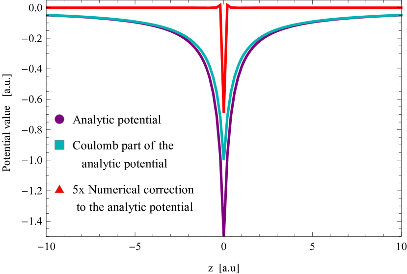
Figure 1: Plot of the analytic potential (21) (in purple) and its regularized Coulomb part (second term of (21), in cyan), for $Z=1$, $\mu=1$. We also plot the difference $\widetilde{V}_{0,{\rm M}}^{{\rm 1D}}(z)-V_{0,{\rm M}}^{{\rm 1D}}(z)$, (see the discussion in section IV) calculated with for $\Delta z=0.2$, and magnified by a factor of 5 (in red). This is to illustrate the numerical correction to be introduced by Eq. (26).

III.2 Improved 1D model potentials

The results of Sec. III.1, especially the somewhat surprising value of an effective charge of $\frac{1}{2}Z$, suggested by the second term of the analytical model potential (21), inspire us to use the 1D soft-core Coulomb potential and a 1D regularized Coulomb potential with accordingly modified values of their parameters. As we will see, these modifications lead indeed to improved results in strong-field simulations.

We use $\frac{1}{2}Z$ in the nominator of the soft-core Coulomb potential, which then requires to change also the parameter $\alpha$ in order to maintain that its ground state energy matches the 3D ground state energy. These lead us to the following formula of the improved 1D soft-core Coulomb potential with $\mu=1$:

$$V_{0,{\rm M,Sc}}^{{\rm 1D}}(z)=-\frac{\frac{1}{2}Z}{\sqrt{z^{2}+\frac{1}{4Z^{2}}}}\text{ with }E_{{\rm 0,M,Sc}}=-\frac{Z^{2}}{2},$$ (22)

that has the correct $\frac{1}{2}Z/|z|$ asymptotic behavior when $|z|\rightarrow\infty$. The energy of its first excited state is $E_{1,{\rm M,Sc}}=-0.1058670$.

We also introduce the improved 1D regularized Coulomb potential as

$$V_{0,{\rm M,C}}^{{\rm 1D}}(z)=-\frac{\frac{1}{2}Z}{|z|+a},$$ (23)

where the value of the parameter $a$ is determined by requiring that the ground state energy is $E_{{\rm 0,M,C}}=-\frac{\mu Z^{2}}{2}$. For $Z=1$ we set $a\approx 0.32889$ which yields $E_{{\rm 0,M,C}}\approx-0.5000007$ (for $\mu=1$). We note that this has been computed numerically with the spatial step size $\Delta z=0.2$.

The sophisticated numerical method to be outlined in the next section will enable us to make additional refinements regarding the 1D density based potential, as well as the 1D delta potential. These improvements will be explained below especially by the formulas given in Eqs. (26) and (27).

IV Numerical methods of the solution

Usually, the time-dependent Schrödinger equation (8) must be solved numerically in the non-perturbative regime. We discretize the time variable with time steps $\Delta t$ as $t_{k}=k\Delta t$, and the spatial coordinate with steps $\Delta z$ as $z_{j}=j\Delta z$ ($k,j$ are integer indices). The discretized wave function is written as $\Psi^{{\rm 1D}}(z_{j},t_{k})$. We write the discretized form of the 1D atomic model Hamiltonian as

$$\widetilde{H}_{0}=\widetilde{T}_{z}+V_{0}^{{\rm 1D}}(z_{j}),$$ (24)

where, based on our experiences detailed in Majorosi and Czirják (2016); Majorosi et al. (2017), we use the following 11-point finite difference method van Dijk and Toyama (2007) for the discretization of the kinetic energy operator $T_{z}$:

$$\widetilde{T}_{z}\Psi(z_{j},t_{k})=-\frac{1}{2\mu}\sum_{s=-5}^{5}c_{|s|}^{(5)}\Psi^{{\rm 1D}}(z_{j}+s\Delta z,t_{k}),$$ (25)

see Table 1 of van Dijk and Toyama (2007) for the coefficients $c$. This is accurate up to $\Delta z^{10}$ for smooth functions (it is also limited by the Fourier representation). Then, the discrete Hamiltonian becomes an 11-banded diagonal matrix which operates on the column vector of the discretized wave function in coordinate representation. Regarding the use of the atomic model potential in numerical simulations, this is the most important step since it defines the numerical eigensystem of the atom.

Regarding the time evolution, we use a 3 step splitting of the $U(t,t+\Delta t)$ evolution operator which has an accuracy of $\Delta t^{4}$, and each of its substeps are propagated using the usual second order Crank-Nicolson method Press et al. (2007) with a discrete second order effective Hamiltonian, the particular formulas can be found in Sec 3.1 and Sec 4.1 in Majorosi and Czirják (2016). We find ground states and ground state energies performing imaginary time propagation Bauer and Koval (2006); Chin et al. (2009). For integrations, we use the quadrature formula $\int f(z){\rm d}z\approx\sum_{j}f(z_{j})\Delta z$ because the numerical time evolution is unitary with respect to this summation.

When using the potential (22) the method described above can be applied without further complications. In the case of our density-based model potential a refinement is necessary as (21) is not differentiable in the origin, just as the true 3D Coulomb potential. Therefore the ground state and energy of the discrete Hamiltonian (24) with $V_{0,{\rm M}}^{{\rm 1D}}(z_{j})$ is accurate only up to $\Delta z^{2}$. This is the reason why its ground state density does not equal $\varrho_{z}^{100}(z_{j})$ accurately enough, unless $\Delta z$ is extremely small. We avoid this inaccuracy in the following way: instead of $V_{0,{\rm M}}^{{\rm 1D}}(z_{j})$, we use its following discretized form in the computations:

$$\widetilde{V}_{0,{\rm M}}^{{\rm 1D}}(z_{j})=E_{0}-\frac{1}{\psi_{0}(z_{j})}\widetilde{T}_{z}\psi_{0}(z_{j}).$$ (26)

This definition of $\widetilde{V}_{0,{\rm M}}^{{\rm 1D}}(z_{j})$ ensures that the discretized ground state vector $\psi_{0}(z_{j})$ is the eigenvector of (24) with $\widetilde{V}_{0,{\rm M}}^{{\rm 1D}}(z_{j})$ and the corresponding energy is $\widetilde{E}_{0,{\rm M}}=E_{0}$, numerically exactly. The energy of the corresponding first excited state (with $\Delta z=0.2$) is $\widetilde{E}_{1,{\rm M}}=-0.0904385$, which is close enough to $E_{1,{\rm M}}$. We have plotted the difference $\widetilde{V}_{0,{\rm M}}^{{\rm 1D}}(z)-V_{0,{\rm M}}^{{\rm 1D}}(z)$ in Fig. 1, magnified by a factor of 5.

The discretized form of the analytical model potential, $\widetilde{V}_{0,{\rm M}}^{{\rm 1D}}(z_{j})$ suggests also a modified discretization of the Dirac-delta potential that we introduce as

$$\widetilde{V}_{0,{\rm DD}}^{{\rm 1D}}(z_{j})=E_{0,{\rm DD}}-\frac{1}{\psi_{0,{\rm DD}}(z_{j})}\widetilde{T}_{z}\psi_{0,{\rm DD}}(z_{j})$$ (27)

using the corresponding exact ground state $\psi_{0,{\rm DD}}(z_{j})$ and energy $E_{0,{\rm DD}}$. This is a finite discretized potential which eliminates any singular feature from the corresponding Hamiltonian matrix. As we show it in Appendix B, such definitions enable consistent and accurate simulations with high order finite differences, therefore it is a valid choice to define a potential using numerical inversion from its ground state.

V Results and comparison of the 1D and 3D calculations

In this section, we present and compare the results of strong-field simulations based on the 1D model potentials discussed in the previous sections. We selected the mean value of the dipole moment $\left\langle z\right\rangle(t)$ and its standard deviation $\sigma_{z}(t)$, the mean value of the velocity $\left\langle v_{z}\right\rangle(t)$, and the ground state population loss $g(t)$ to characterize the dynamics resulting from the solutions of (8) with the various model potentials and from the solution of (6) as a reference. We also investigate the relation between the resulting various dipole power spectra $p(f)$, which is one of the most important quantities for high order harmonic generation McPherson et al. (1987); Harris et al. (1993); Lewenstein et al. (1994) and attosecond pulses. For the formulas of these physical quantities and for some details about the numerical accuracy of the simulations, see Appendix A and B.

In these simulations, we model the linearly polarized few-cycle laser pulse with a sine-squared envelope function. The corresponding time-dependent electric field has non-zero values only in the interval $0\leq t\leq N_{\text{Cycle}}T$ according to the formula:

$$\mathcal{E}_{z}(t)=F\cdot\sin^{2}\left(\frac{\pi t}{2N_{\text{Cycle}}T}\right)\cos\left(\frac{2\pi t}{T}\right),$$ (28)

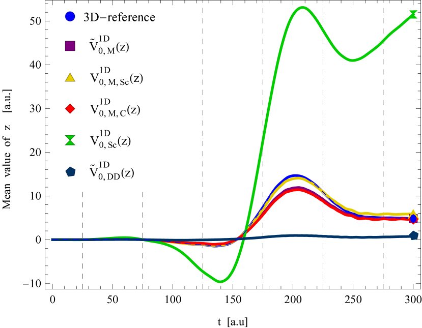
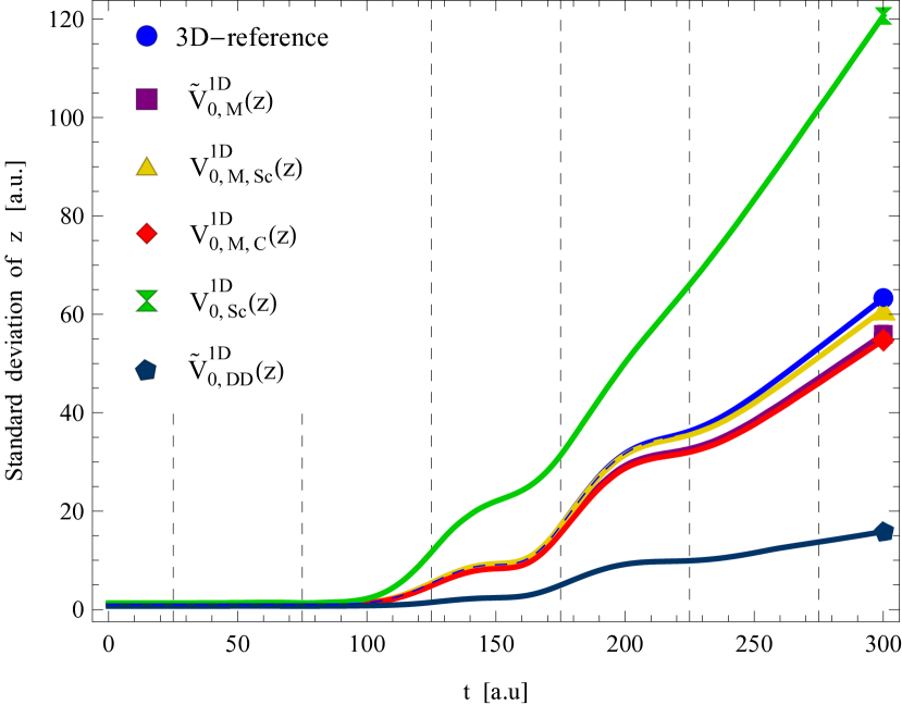
Figure 2: Time-dependence of the mean values $\left\langle z\right\rangle(t)$ (a) and the standard deviations $\sigma_{z}(t)$ (b) using different 1D model potentials, under the influence of the same external field with $F=0.1$, $N_{\text{Cycle}}=3$ and $T=100$. Results of the corresponding 3D simulation are plotted in blue.

where $T$ is the period of the carrier wave, $F$ is the peak electric field strength and $N_{\text{Cycle}}$ is the number of cycles under the envelope function. Unless otherwise stated, we set $N_{\text{Cycle}}=3$ and $T=100$, the latter corresponds to a ca. $725\,\mathrm{nm}$ near-infrared carrier wavelength. From Fig. 2 on, the vertical dashed lines denote the zero crossings of the respective $\mathcal{E}_{z}(t)$ electric field.

We consider hydrogen in most of the simulations, i.e. we use $Z=1$ and $\mu=1$ if not otherwise stated explicitly. We set typically $\Delta z=0.2$ and $\Delta t=0.01$ since these are sufficient for the numerical errors to be within line thickness. We use box boundary conditions and we set the size of the box to be sufficiently large so that the reflexions are kept below $10^{-8}$ atomic units.

The 3D reference results (i.e. the simulation results of the true 3D Schrödinger equation (6)) are plotted in Figs. 2 to 8 in blue and are labeled “3D reference”. The 1D simulation results and their respective colors are plotted as follows: our density-based model potential from numerical inversion (26) in purple, our improved soft-core Coulomb potential (22) in gold, our improved regularized Coulomb potential (23) in red, the conventional soft-core Coulomb potential (9) in green and the discretized Dirac-delta potential (11) in dark blue.

V.1 Low frequency response

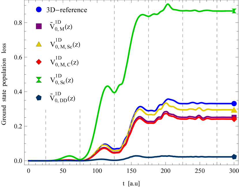
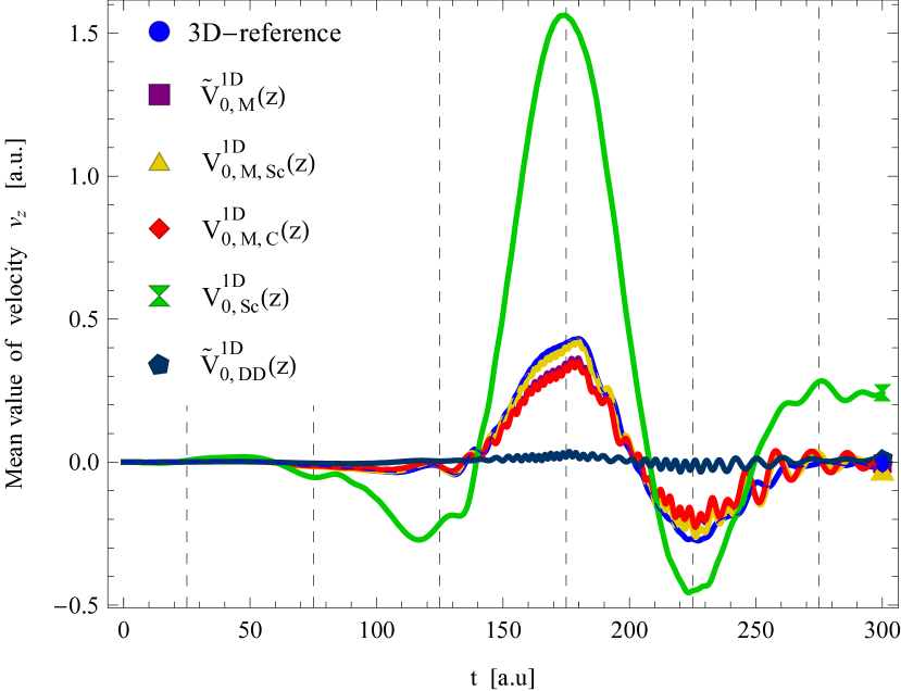
Figure 3: Time-dependence of the ground state population loss $g(t)$ (a) and the mean velocities $\left\langle v_{z}\right\rangle(t)$ (b) using different 1D model potentials, under the influence of the same external field with $F=0.1$, $N_{\text{Cycle}}=3$ and $T=100$. Results of the corresponding 3D simulation are plotted in blue.

First, we discuss the results of a moderately strong laser pulse having a peak electric field value of $F=0.1$. We plot the corresponding time-dependent mean values $\left\langle z\right\rangle(t)$ (the magnitude of which equals the dipole moment in atomic units) and their standard deviations $\sigma_{z}(t)$ in Fig. 2, the time-dependent mean velocities $\left\langle v_{z}\right\rangle(t)$ and the ground state population losses $g(t)$ in Fig. 3 for all the 1D model systems listed above. These curves justify that the simulation results obtained with our density-based model potential and the improved model potentials are already quantitatively comparable to the 3D results, i.e. these model potentials capture the essence of the 3D process. This fact is in strong contrast with the poor results of the conventional 1D soft-core and 1D Dirac-delta potentials, which is caused mainly by their too weak and too strong binding force, respectively.

The graphs of the improved soft-core Coulomb potential are clearly at the closest to the 3D reference in most of these cases, i.e. this potential provides the quantitatively best model of the 3D case, despite that its ground state density is not the exact reduced density of the 3D case. The results of our numerical density-based model potential are somewhat less close to the 3D reference. Although these simulations start from the exact reduced density of the 3D case, the electron is somewhat stronger bound to the ion-core than optimal. The results obtained using the improved regularized Coulomb potential are very close to those of the density-based model potential, but the former potential is even somewhat stronger than needed.

In a typical strong-field simulation, the ground state population loss $g(t)$ is close to the probability of ionization. Due to the presence of the transverse degrees of freedom in 3D, it is then reasonable that the $g(t)$ values are somewhat larger in a 3D simulation than in 1D. Note that the $g(t)$ curves of the 1D simulations follow very well the 3D reference curve in accordance with this.

The lack of the transverse degrees of freedom affects the $\left\langle v_{z}\right\rangle(t)$ curves of the 1D simulations in a different way: These exhibit the high-frequency oscillations with larger amplitude than the 3D reference curve. This can be explained by taking into account that rescattering on the ion-core is a much stronger factor in 1D, and that the integration over the transverse directions decreases the effect of the 3D density oscillations on the reduced mean values. We will analyze this in more detail in the next subsection.

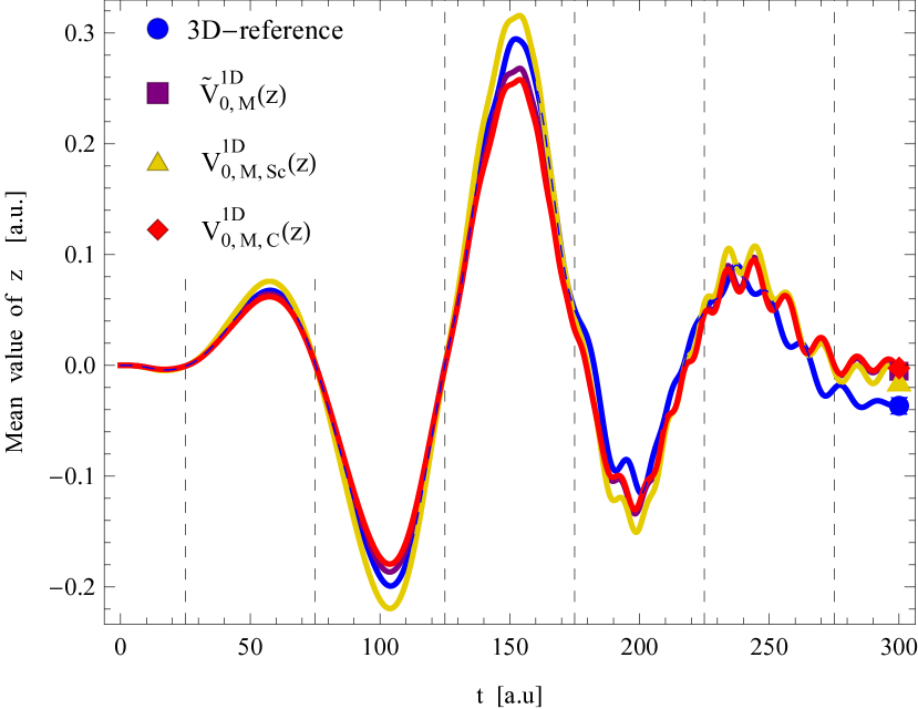
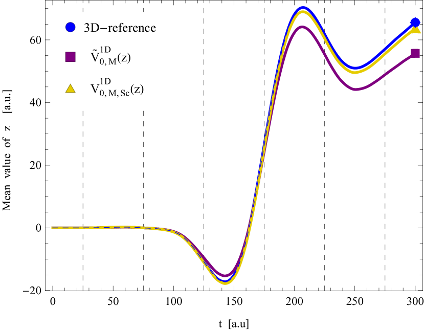
Figure 4: Time-dependence of mean values $\left\langle z\right\rangle(t)$ using different 1D model potentials, under the influence of the external field with $F=0.05$ (a) and $F=0.15$ (b), $N_{\text{Cycle}}=3$ and $T=100$. Results of the corresponding 3D simulations are plotted in blue.

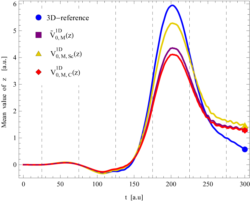
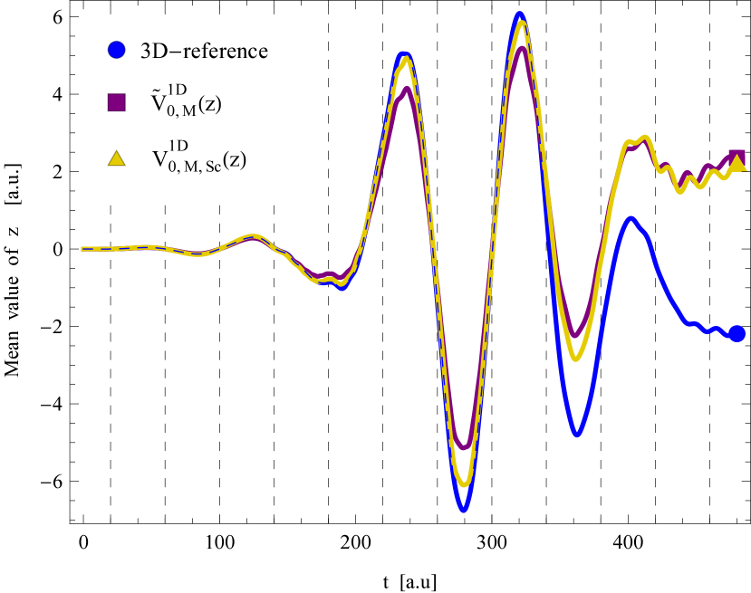
Figure 5: Time-dependence of mean values $\left\langle z\right\rangle(t)$ using different 1D model potentials. Panel (a): single active electron model of a neon atom with $Z_{{\rm Ne}}^{{\rm(SAE)}}=1.25929$, driven by the external field with $T=100$, $F=0.15$, $N_{\text{Cycle}}=3$. Panel (b): hydrogen with $Z=1$ using the driven by the external field with $T=80$, $F=0.1$, $N_{\text{Cycle}}=6$. Results of the corresponding 3D simulations are plotted in blue.

In order to demonstrate the capabilities of these novel 1D model potentials, we selected the time-dependent dipole moment $\left\langle z\right\rangle(t)$ to present the results of 4 different scenarios in Fig. 4 and Fig. 5. Since the curves corresponding to the density-based model potential are very close to those corresponding to the improved regularized 1D Coulomb potential, we do not plot the $\left\langle z\right\rangle(t)$ of this latter potential in all of our Figures.

In Fig. 4 (a) we plot our simulation results for hydrogen, now with a weaker field of $F=0.05$ which is in the tunnel ionization regime of hydrogen, while Fig. 4 (b) corresponds to a stronger field of $F=0.15$. Both of these figures clearly show that the improved 1D soft-core Coulomb potential provides the best results. Note that the change of $F$ in the above range results in more than 2 orders of magnitude change in the peak value of $\left\langle z\right\rangle(t)$.

Fig. 5 (a) shows the results for a Ne atom driven by a field of $F=0.15$. Here we model the 3D Neon atom in the single active electron approximation Lewenstein et al. (1994) simply by setting the Coulomb-charge $Z_{{\rm Ne}}^{{\rm(SAE)}}=1.25929$ in order to match the ionization potential to the experimental value. (For the improved regularized Coulomb potential $V_{0,{\rm M,C}}^{{\rm 1D}}$ we set $a_{{\rm Ne}}^{({\rm SAE)}}\approx 0.26707525$ which yields $E_{{\rm 0,M,C}}\approx-0.792905$.)

The accuracy of these 1D results is somewhat lower around the peak and in the last half-period of the laser pulse than in the case of hydrogen, and the improved soft-core Coulomb potential performs considerably better in overall than the two other model potentials. By changing the Coulomb charge $Z$ within a reasonable range in order to model different noble gas atoms, we have obtained similarly accurate results.

Fig. 5 (b) shows $\left\langle z\right\rangle(t)$ for a hydrogen atom, now driven by a longer laser pulse of shorter carrier wavelength, corresponding to the parameters $T=80$, $F=0.1$, and $N_{\text{Cycle}}=6$. The 1D model potentials work similarly accurately for this longer laser pulse as in the case presented in Fig. 2 (b), until the recollisions with the ion-core gradually decrease the match between the 1D and 3D cases in the last 2 periods of the pulse.

Our density-based 1D model potential and both of the improved 1D model potentials exhibit an impressive improvement in the accuracy of the low-frequency response of typical strong-field processes, in contrast to the two conventional model potentials. These results are even more convincing if we take into account that $\left\langle z\right\rangle(t)$, $\sigma_{z}(t)$ and $g(t)$ are very sensitive to almost any change in the physical parameter values.

V.2 High order harmonic spectra

In strong-field physics, the accurate computation of the high order harmonic spectrum is especially important, because this represents the highly nonlinear atomic response to the strong-field excitation, with well-known characteristic features McPherson et al. (1987); Ferray et al. (1988); Harris et al. (1993); Krausz and Ivanov (2009); Gombkötő et al. (2016). Besides the high-order harmonic yield, the suitable phase relations enable to generate attosecond pulses of XUV light Farkas and Tóth (1992); Paul et al. (2001); Hentschel et al. (2001); Drescher et al. (2002); Kienberger et al. (2002); Carrera et al. (2006); Sansone et al. (2006).

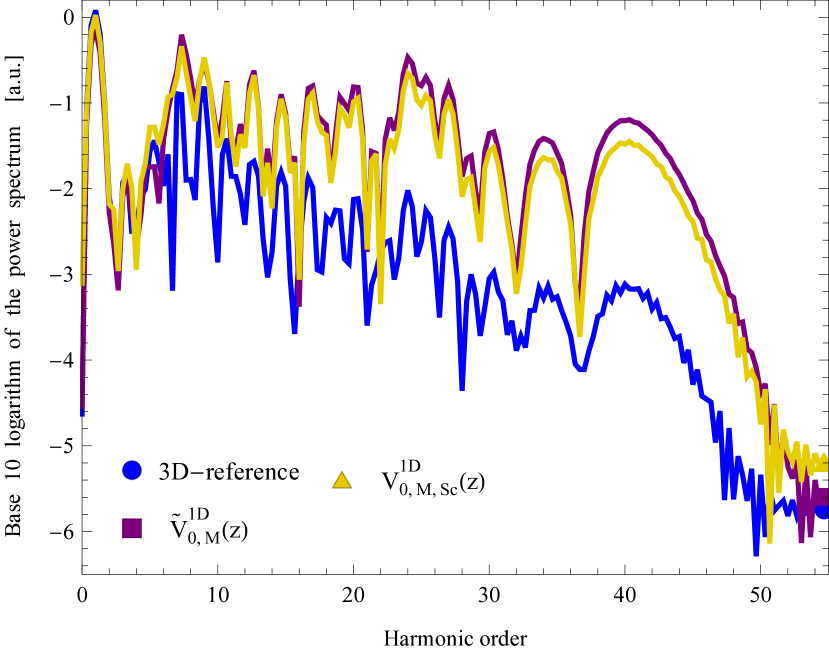
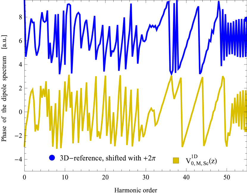
Figure 6: Panel (a): Logarithmic plot of the power spectra vs. the harmonic order, i.e. $p(nf_{1})$ (where $f_{1}=1/T=0.01$ a.u. is the fundamental frequency). Panel (b): Phase of the dipole acceleration spectra vs. the harmonic order (up shifted by $2\pi$ for the 3D case). We plot the results for the density-based 1D model potential (purple) and for the improved soft-core Coulomb potential (gold) in comparison with the 3D reference (blue). The parameters $F=0.1$, $N_{\text{Cycle}}=3$, $T=100$ and $Z=1$ are the same as for Figs. 2 and 3.

In Fig. 6 (a), we plot the power spectrum of the dipole acceleration (see Eq. 36) for the parameters corresponding to Figs. 2 and 3.

In agreement with the previous subsection, the power spectra obtained using the 1D model potentials agree very well with the 3D reference simulation result up to the 5th harmonic. For higher frequencies, the 1D spectra gradually deviate and give 1-2 orders of magnitude larger values than the 3D reference values. The explanation given for the oscillations of the $\left\langle v_{z}\right\rangle(t)$ curves in Fig. 3 (b) applies also here: 1D simulations exaggerate the effect of the ion-core, mainly via rescattering, while the effect of the 3D density oscillations weakens in the reduced mean values obtained from the 3D simulation.

However, the structure of the spectra in Fig. 6 (a) is remarkably similar and the match of the spectral phase, shown in Fig. 6 (b), is very good, especially in the higher frequency range, which is of fundamental importance for isolated attosecond pulses. These inspired us to create a scaling function which transforms the spectra obtained with the 1D simulation to fit the 3D reference spectrum as correctly as possible. Since the improved soft-core Coulomb potential (22) gives the best low-frequency results, we focus only on this model potential in the following.

Examination of the ratio of the magnitudes of the 1D power spectrum to the 3D power spectrum in our simulations with different parameters revealed that the scaling function

$$s(f)=\min\left(1+0.03\left(100f-1\right)^{2},1+\left|100f-1\right|\right)$$ (29)

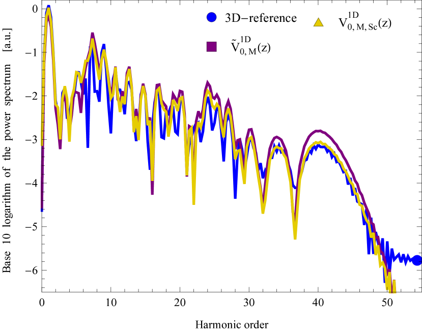
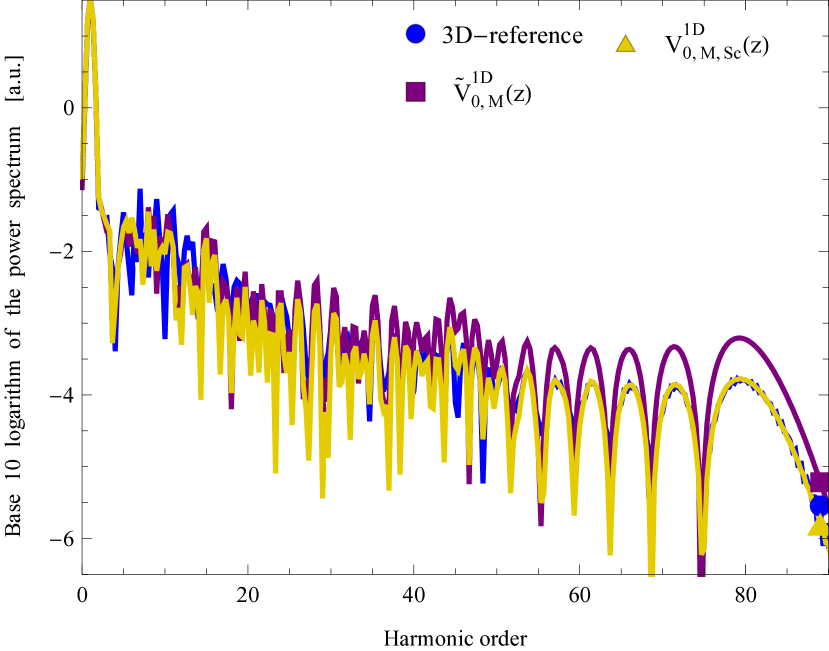
Figure 7: Logarithmic plots of the scaled power spectra $p(nf_{0})/s(nf_{0})$ using the model systems of Fig. 6 with $F=0.10$ (a), $F=0.15$ (b), in comparison with the 3D reference (blue).

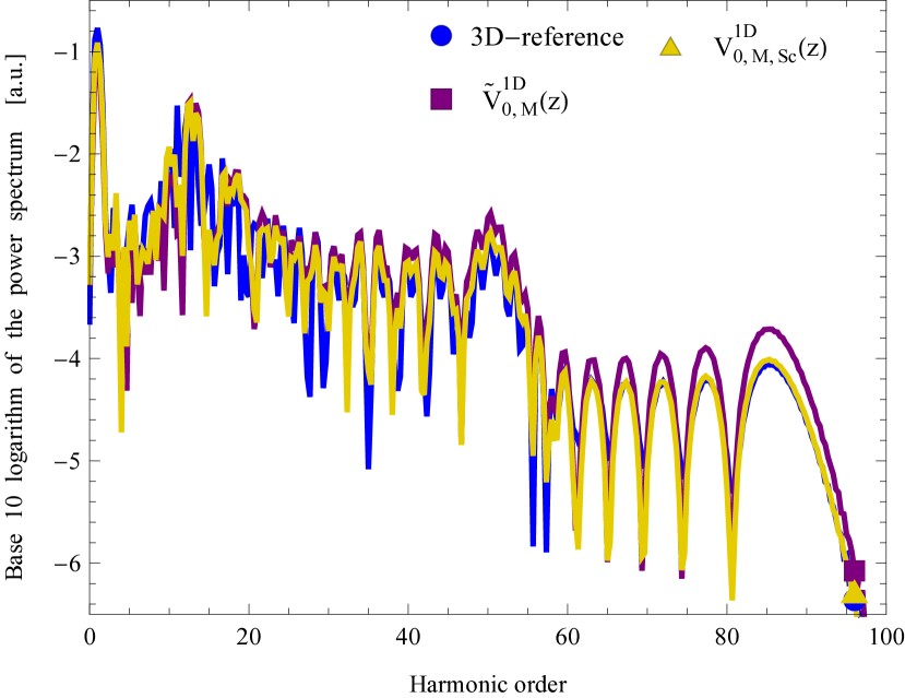
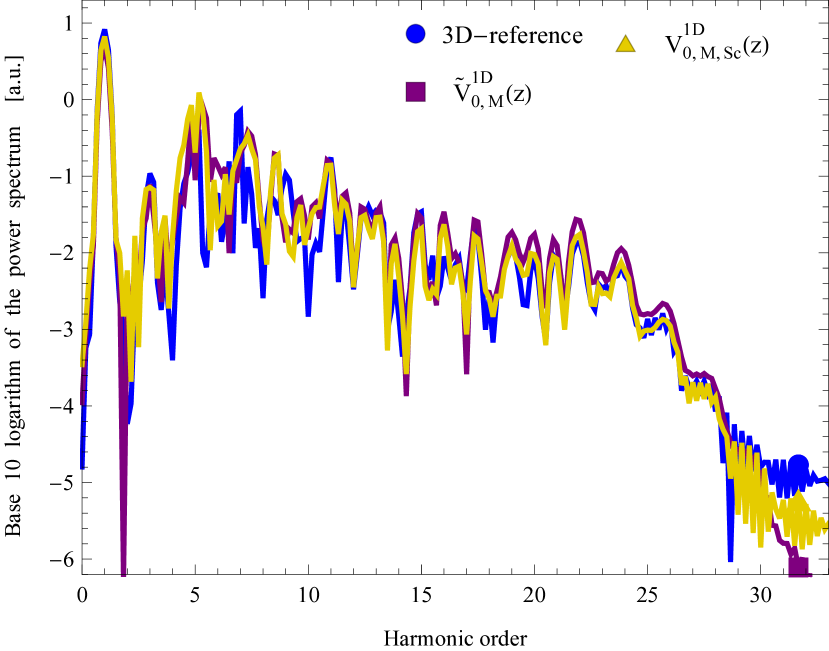
Figure 8: Logarithmic plots of the scaled power spectra $p(nf_{0})/s(nf_{0})$ obtained using the density-based 1D model potential (purple) and the improved soft-core Coulomb potential (gold), in comparison with the 3D reference (blue). Panel (a): single active electron model of a neon atom with $Z_{{\rm Ne}}^{{\rm(SAE)}}=1.25929$ driven by the external field with $T=100$, $F=0.15$, $N_{\text{Cycle}}=3$. Panel (b): hydrogen with $Z=1$, driven by the external field with $T=80$, $F=0.1$, $N_{\text{Cycle}}=6$.

transforms the magnitude of the power spectra obtained using the improved 1D soft-core Coulomb potential to properly fit the corresponding 3D power spectra. In Fig. 7 (a) we plot the scaled 1D power spectrum $p(f)/s(f)$ which gives a very good match between the 3D and 1D results in the case of the improved soft-core Coulomb potential. (Here and in the following figures we plot the scaled power spectrum of the density-based 1D model potential for completeness only.) In Fig. 7 (b) and Fig. 8 (a) and (b) we present this comparison for three other scenarios, corresponding to the parameters of Fig. 4 (b) and Fig. 5 (a) and (b), respectively. These plots clearly show that the scaling function (29) works very well also in these cases.

VI Discussion and conclusions

The results presented in the previous section demonstrate that it is possible to quantitatively model the true 3D quantum dynamics with the help of the density-based 1D model potential $\widetilde{V}_{0,{\rm M}}^{{\rm 1D}}(z_{j})$ and the accordingly improved soft-core Coulomb potential $V_{0,{\rm M,Sc}}^{{\rm 1D}}(z)$. The best results are obtained with the improved soft-core Coulomb potential (22) which is also very easy to use numerically. This means that we can perform quantum simulations of a single active electron atom driven by a strong linearly polarized laser pulse during a couple of minutes and obtain a fairly accurate low-frequency response and a reliable HHG spectrum with the help of the scaling function (29). The simple form of this scaling is based on the good agreement between the structure and phase of the 1D and the 3D HHG spectra.

In achieving these results, the physical requirement about the 1D and 3D ground state densities was the important starting idea. This led to the construction of the density-based 1D model potential, which then inspired the improved parametrization of the 1D soft-core Coulomb potential with effective charge $\frac{1}{2}Z$. Both of these have the same asymptotic tail which ensures that their ground state energy is identical to that of the 3D system. The discretization of the density-based 1D model potential gave important lessons also about the numerical aspects of non-differentiable 1D Coulomb-like potentials and the 1D delta potential.

Considering the obvious differences between the 1D and the 3D quantum dynamics and their effects, discussed already in connection with Figs. 3 (b) and 6 (a), it is not surprising that the high-frequency response of these 1D simulations is much stronger than that of the corresponding 3D case. The fact that the scaling function (29) has different frequency-dependence in the lower frequency domain than in the higher frequency domain, and that this seems to be independent of the other physical parameters, may hint at a deeper connection between the true 3D quantum dynamics and its best 1D model given by the improved soft-core Coulomb potential (22).

We expect that this improved soft-core Coulomb potential can be successfully used as a building block also in the 1D model of somewhat larger atomic systems, like a He atom, driven by a strong linearly polarized laser pulse. The method of construction of the reduced density-based 1D model potential could be used as well to create proper 1D model potentials for strong-field simulation of simple molecules, like $\mathrm{H}_{2}^{+}$ or $\mathrm{H}_{2}$.

Appendix A Comparable physical quantities in 1D

For completeness, we list here the physical quantities that we use for characterizing the strong-field process, both in 1D and 3D.

From the 3D wave function we can calculate the 1D reduced density as

$$\varrho_{z}^{{\rm 3D}}(z,t)=2\pi\int_{0}^{\infty}\left|\Psi^{{\rm 3D}}(z,\rho,t)\right|^{2}\rho\text{d}\rho.$$ (30)

In 1D this is

$$\varrho_{z}^{{\rm 1D}}(z,t)=\left|\Psi^{{\rm 1D}}(z,t)\right|^{2}.$$ (31)

We calculate the mean value of $z$ as

$$\left\langle z\right\rangle(t)=\int_{-\infty}^{\infty}z\varrho_{z}(z,t)\text{d}z,$$ (32)

the standard deviation of $z$ as

$$\sigma_{z}(t)=\sqrt{\left\langle z^{2}\right\rangle(t)-\left\langle z\right\rangle^{2}(t)},$$ (33)

the mean value of the $z$-velocity and the $z$-acceleration using the Ehrenfest theorems as

$$\left\langle v_{z}\right\rangle(t)=\frac{\partial\left\langle z\right\rangle}{\partial t},\,\,\,\,\,\,\,\left\langle a_{z}\right\rangle(t)=\frac{\partial\left\langle v_{z}\right\rangle}{\partial t},$$ (34)

in both the 3D and the 1D cases. It is also interesting to determine the ground state population loss

$$g(t)=1-\left|\left\langle\Psi(0)|\Psi(t)\right\rangle\right|^{2},$$ (35)

even though this refers to the population losses of two completely different states in 1D and 3D.

We calculate the spectrum from the dipole acceleration $\left\langle a_{z}\right\rangle$, and then the power spectrum as

$$p(f)=\left|\mathcal{F}\left[\left\langle a_{z}\right\rangle\right](f)\right|^{2}$$ (36)

where $\mathcal{F}$ denotes the Fourier transform and $f$ is its frequency variable.

Appendix B Accuracy of the numerical inversion

B.1 Density-based 1D model potential

We stated previously that the numerical construction (26) yields the exact numerical eigensystem of that potential, but that does not give us the whole picture about how numerically accurate the construction really is. If we look at the eigenenergy of its respective first excited state calculated with $\Delta z=0.2$ we see that it is 4-5 digit accurate, but that alone does not determine the usefulness in strong-field simulations. To get the whole picture, we performed some numerical simulations using the atomic potential (26) and a 3-cycle laser pulse of form (28) with $F=0.1$ with different $\Delta z$ parameters. We subtracted from them the results of a very accurate reference numerical solution using the analytical potential (21) with $\Delta z=0.0001$, which gave us information about the (approximate) numerical errors of the construction.

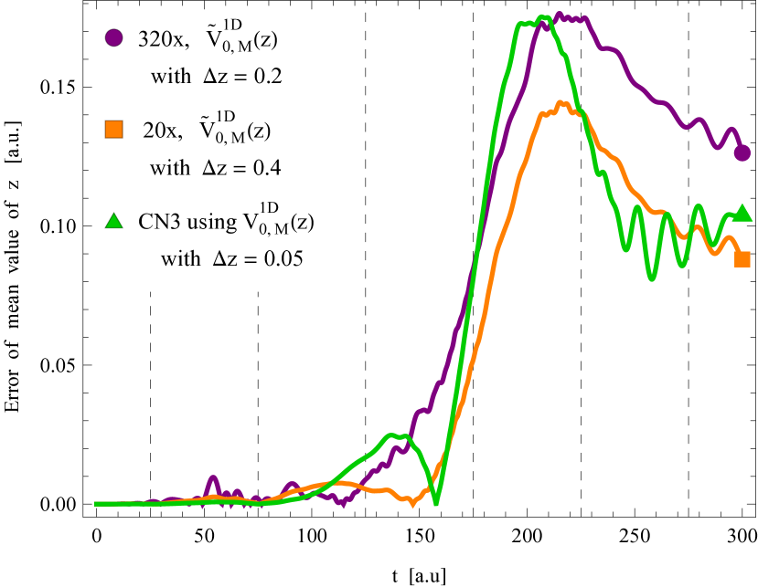
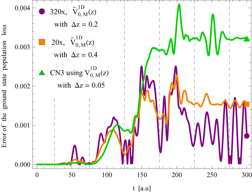
Figure 9: Time-dependence of the numerical mean value errors $\left|\left\langle z\right\rangle(t)-\left\langle z\right\rangle_{\text{num,ref}}(t)\right|$ (a) and ground state population loss errors $\left|g(t)-g_{\text{num,ref}}(t)\right|$ (b) using different realizations of the density-based model potentials, under the influence of the same external field with $F=0.1$, $N_{\text{Cycle}}=3$. We plotted in purple and orange the results using the potential $\widetilde{V}_{0,{\rm M}}^{{\rm 1D}}$ from numerical inversion formula (26) with $\Delta z=0.2$, and $\Delta z=0.4$, respectively. Note that the values of these two curves are magnified by a factor of 320 and 20 as indicated. For comparison, we plotted in green the results directly using the analytic formula (21) as the atomic potential in an usual Crank-Nicolson solution.

The results can be seen on Fig. 9, where we plotted the errors of mean values $\left\langle z\right\rangle(t)$ and the ground state population losses $g(t)$ compared to reference versus time. We can see that if we decrease the spatial step $\Delta z$ of the inversion (26) from 0.4 (orange) to 0.2 (purple) the error decreases approximately by a factor of 16, in the case of both $\left\langle z\right\rangle(t)$ and $g(t)$. We verified this using also other integrated quantities: we can clearly assert that the numerical inversion (26) is around $\Delta z^{4}$ accurate i.e. it shows high order accuracy (required that the kinetic energy operator is also at least $\Delta z^{4}$ accurate). To illustrate what this means, we also plotted the results obtained by the usual 3-point finite difference Crank-Nicolson method (CN3) using the analytical potential (21) as the atomic potential, which are known to be $\Delta z^{2}$ accurate. We briefly note that we tested the direct use of (21) with our 11-point finite difference scheme but it was not any better, also $\Delta z^{2}$ accurate (since the potential is not differentiable), so we only plotted the results of the CN3 scheme in Fig. 9 with green lines. The accuracy of this method using $\Delta z=0.2$ is around 320 times better than the direct use of the analytical non-differentiable potential with $\Delta z=0.05$. So in other words it requires $2^{6}$ more spatial gridpoints ($\Delta z\approx 0.003$) than the numerical inversion. Using the formula (26) to numerically represent the (nonsingular) model potentials is very efficient and shows high order convergence.

B.2 Delta potential

In the following, we discuss the accuracy tests of the numerically constructed potential (27) using strong-field simulations with the same 3-cycle laser pulse of form (28) with $F=0.1$ and different $\Delta z$ parameters. For comparison we use a properly implemented method from Czirják et al. (2013) that uses the proper Robin boundary condition at $z=0$, which overrides the Crank-Nicolson equations at that grid point. Its results are at least $\Delta z^{2}$ accurate. We calculate the errors of the mean values $\left\langle z\right\rangle(t)$ and the ground state population losses $g(t)$ compared to a very accurate reference solution obtained by this correct method (uses $\Delta z=0.001$). We can see the results on Fig. 10. Surprisingly, we can observe that the errors of (27) with $\Delta z=0.2$ are actually not far from the errors of results obtained by the $\Delta z^{2}$ accurate proper method at $\Delta z=0.05$. If we decrease the $\Delta z$ step from 0.4 (orange) to 0.2 (dark blue) we see a factor 4 error decrease: we can conclude that the non-singular construction (27) is actually correct numerical representation, and converges with $\Delta z^{2}$ even for the singular delta potential. It is also of importance because of the following: we can run simulations with singular potentials using non-singular Hamiltonians, and the point of singularity is not have to be on the spatial grid, it can even move. It has even more interesting consequences in 2D or more, since there is no reason not to work with the true singular Coulomb potentials.

In conclusion, it is a valid choice to define potentials using numerical inversion from its ground state. It can provide a consistent and accurate method with high order finite differences to represent our (21) non-singular and non-differentiable atomic potential in 1D, and even achieve $\Delta z^{4}$ convergence. The method is robust enough to provide $\Delta z^{2}$ convergence for the case of the singular 1D delta potential using (27).

(a)                                                                           (b)

(a)                                                                           (b)

(a)                                                                           (b)

(a)                                                                           (b)

(a)                                                                           (b)

(a)                                                                           (b)

(a)                                                                           (b)

(a)                                                                           (b)

(a)                                                                           (b)

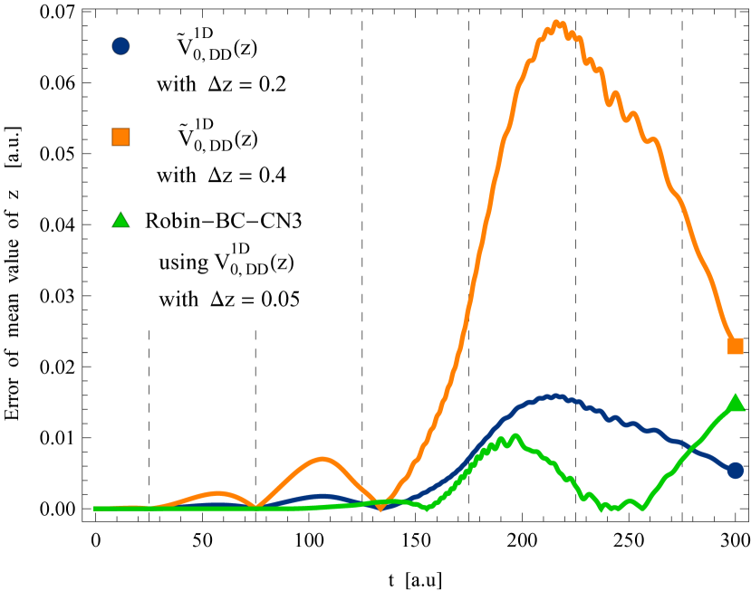
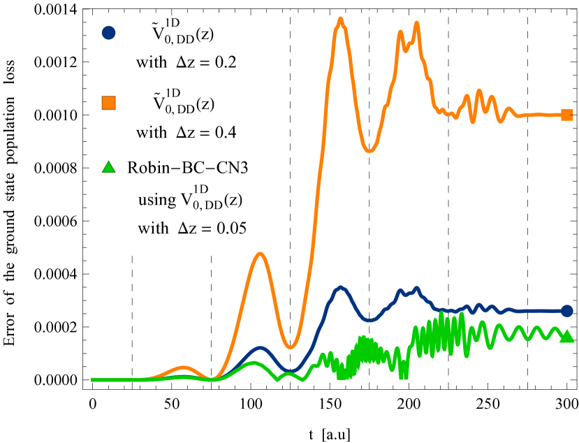
Figure 10: Time-dependence of the numerical mean value errors $\left|\left\langle z\right\rangle(t)-\left\langle z\right\rangle_{\text{num,ref}}(t)\right|$ (a) and ground state population loss errors $\left|g(t)-g_{\text{num,ref}}(t)\right|$ (b) using different implementations of the Dirac-delta model potential, under the influence of the same external field with $F=0.1$, $N_{\text{Cycle}}=3$. We plotted in dark blue and orange the results using the potential $\widetilde{V}_{0,{\rm DD}}^{{\rm 1D}}$ from numerical inversion formula (27) with $\Delta z=0.2$, and $\Delta z=0.4$, respectively. For comparison, we plotted in green the results using the implementation in Czirják et al. [2013] that uses the proper Robin boundary condition to represent the singularity of (11).

References

- Hentschel et al. [2001] M Hentschel, R Kienberger, Ch Spielmann, Georg A Reider, N Milosevic, Thomas Brabec, Paul Corkum, Ulrich Heinzmann, Markus Drescher, and Ferenc Krausz. Attosecond metrology. Nature, 414(6863):509–513, 2001.
- Kienberger et al. [2002] Reinhard Kienberger, Michael Hentschel, Matthias Uiberacker, Ch Spielmann, Markus Kitzler, Armin Scrinzi, M Wieland, Th Westerwalbesloh, U Kleineberg, Ulrich Heinzmann, et al. Steering attosecond electron wave packets with light. Science, 297(5584):1144–1148, 2002.
- Drescher et al. [2002] Markus Drescher, Michael Hentschel, R Kienberger, Matthias Uiberacker, Vladislav Yakovlev, Armin Scrinzi, Th Westerwalbesloh, U Kleineberg, Ulrich Heinzmann, and Ferenc Krausz. Time-resolved atomic inner-shell spectroscopy. Nature, 419(6909):803–807, 2002.
- Baltuška et al. [2003] Andrius Baltuška, Th Udem, M Uiberacker, M Hentschel, E Goulielmakis, Ch Gohle, Ronald Holzwarth, VS Yakovlev, A Scrinzi, TW Hänsch, et al. Attosecond control of electronic processes by intense light fields. Nature, 421(6923):611–615, 2003.
- Uiberacker et al. [2007] Matthias Uiberacker, Th Uphues, Martin Schultze, Aart Johannes Verhoef, Vladislav Yakovlev, Matthias F Kling, Jens Rauschenberger, Nicolai M Kabachnik, Hartmut Schröder, Matthias Lezius, et al. Attosecond real-time observation of electron tunnelling in atoms. Nature, 446(7136):627–632, 2007.
- Krausz and Ivanov [2009] Ferenc Krausz and Misha Ivanov. Attosecond physics. Reviews of Modern Physics, 81(1):163–234, 2009.
- Hommelhoff et al. [2009] Peter Hommelhoff, Catherine Kealhofer, Anoush Aghajani-Talesh, Yvan RP Sortais, Seth M Foreman, and Mark A Kasevich. Extreme localization of electrons in space and time. Ultramicroscopy, 109(5):423–429, 2009.
- Schultze et al. [2010] Martin Schultze, Markus Fieß, Nicholas Karpowicz, Justin Gagnon, Michael Korbman, Michael Hofstetter, S Neppl, Adrian L Cavalieri, Yannis Komninos, Th Mercouris, et al. Delay in photoemission. Science, 328(5986):1658–1662, 2010.
- Haessler et al. [2010] Stefan Haessler, J Caillat, W Boutu, C Giovanetti-Teixeira, T Ruchon, T Auguste, Z Diveki, P Breger, A Maquet, B Carré, et al. Attosecond imaging of molecular electronic wavepackets. Nature Physics, 6(3):200–206, 2010.
- Pfeiffer et al. [2012] Adrian N Pfeiffer, Claudio Cirelli, Mathias Smolarski, Darko Dimitrovski, Mahmoud Abu-Samha, Lars Bojer Madsen, and Ursula Keller. Attoclock reveals natural coordinates of the laser-induced tunnelling current flow in atoms. Nature Physics, 8(1):76–80, 2012.
- Shafir et al. [2012] Dror Shafir, Hadas Soifer, Barry D Bruner, Michal Dagan, Yann Mairesse, Serguei Patchkovskii, Misha Yu Ivanov, Olga Smirnova, and Nirit Dudovich. Resolving the time when an electron exits a tunnelling barrier. Nature, 485(7398):343–346, 2012.
- Ranitovic et al. [2014] Predrag Ranitovic, Craig W Hogle, Paula Rivière, Alicia Palacios, Xiao-Ming Tong, Nobuyuki Toshima, Alberto González-Castrillo, Leigh Martin, Fernando Martín, Margaret M Murnane, et al. Attosecond vacuum uv coherent control of molecular dynamics. Proceedings of the National Academy of Sciences, 111(3):912–917, 2014.
- Peng et al. [2015] Liang-You Peng, Wei-Chao Jiang, Ji-Wei Geng, Wei-Hao Xiong, and Qihuang Gong. Tracing and controlling electronic dynamics in atoms and molecules by attosecond pulses. Physics Reports, 575:1–71, 2015.
- Ciappina et al. [2017] Marcello F Ciappina, JA Pérez-Hernández, AS Landsman, WA Okell, Sergey Zherebtsov, Benjamin Förg, Johannes Schötz, L Seiffert, T Fennel, T Shaaran, et al. Attosecond physics at the nanoscale. Reports on Progress in Physics, 80(5):054401, 2017.
- Keldysh [1965] LV Keldysh. Ionization in the field of a strong electromagnetic wave. Soviet Physics JETP, 20(5):1307–1314, 1965.
- Varró and Ehlotzky [1993] Sándor Varró and F Ehlotzky. A new integral equation for treating high-intensity multiphoton processes. Il Nuovo Cimento D, 15(11):1371–1396, 1993.
- Lewenstein et al. [1994] Maciej Lewenstein, Ph Balcou, M Yu Ivanov, A L’Huillier, and Paul B Corkum. Theory of high-harmonic generation by low-frequency laser fields. Physical Review A, 49(3):2117, 1994.
- Protopapas et al. [1997] M Protopapas, DG Lappas, and PL Knight. Strong field ionization in arbitrary laser polarizations. Physical Review Letters, 79(23):4550, 1997.
- Ivanov et al. [2005] Misha Yu Ivanov, Michael Spanner, and Olga Smirnova. Anatomy of strong field ionization. Journal of Modern Optics, 52(2-3):165–184, 2005.
- Gordon et al. [2005] Ariel Gordon, Robin Santra, and Franz X Kärtner. Role of the Coulomb singularity in high-order harmonic generation. Physical Review A, 72(6):063411, 2005.
- Frolov et al. [2012] MV Frolov, NL Manakov, AM Popov, OV Tikhonova, EA Volkova, AA Silaev, NV Vvedenskii, and Anthony F Starace. Analytic theory of high-order-harmonic generation by an intense few-cycle laser pulse. Physical Review A, 85(3):033416, 2012.
- Javanainen et al. [1988] Juha Javanainen, Joseph H Eberly, and Qichang Su. Numerical simulations of multiphoton ionization and above-threshold electron spectra. Physical Review A, 38(7):3430, 1988.
- Su and Eberly [1991] Q Su and JH Eberly. Model atom for multiphoton physics. Physical Review A, 44(9):5997, 1991.
- Bauer [1997] D Bauer. Two-dimensional, two-electron model atom in a laser pulse: Exact treatment, single-active-electron analysis, time-dependent density-functional theory, classical calculations, and nonsequential ionization. Physical Review A, 56(4):3028, 1997.
- Chirilă et al. [2010] CC Chirilă, Ingo Dreissigacker, Elmar V van der Zwan, and Manfred Lein. Emission times in high-order harmonic generation. Physical Review A, 81(3):033412, 2010.
- Silaev et al. [2010] AA Silaev, M Yu Ryabikin, and NV Vvedenskii. Strong-field phenomena caused by ultrashort laser pulses: Effective one-and two-dimensional quantum-mechanical descriptions. Physical Review A, 82(3):033416, 2010.
- Sveshnikov and Khomovskii [2012] Konstantin Alekseevich Sveshnikov and Dmitrii Igorevich Khomovskii. Schrödinger and Dirac particles in quasi-one-dimensional systems with a Coulomb interaction. Theoretical and Mathematical Physics, 173(2):1587–1603, 2012.
- Gräfe et al. [2012] Stefanie Gräfe, Jens Doose, and Joachim Burgdörfer. Quantum phase-space analysis of electronic rescattering dynamics in intense few-cycle laser fields. Journal of Physics B: Atomic, Molecular and Optical Physics, 45(5):055002, 2012.
- Czirják et al. [2000] A Czirják, R Kopold, W Becker, M Kleber, and WP Schleich. The Wigner function for tunneling in a uniform static electric field. Optics communications, 179(1):29–38, 2000.
- Czirják et al. [2013] Attila Czirják, Szilárd Majorosi, Judit Kovács, and Mihály G Benedict. Emergence of oscillations in quantum entanglement during rescattering. Physica Scripta, 2013(T153):014013, 2013.
- Geltman [2011] Sydney Geltman. Bound states in delta function potentials. Journal of Atomic, Molecular, and Optical Physics, 2011, 2011.
- Baumann et al. [2015] C Baumann, H-J Kull, and GM Fraiman. Wigner representation of ionization and scattering in strong laser fields. Physical Review A, 92(6):063420, 2015.
- Teeny et al. [2016] Nicolas Teeny, Enderalp Yakaboylu, Heiko Bauke, and Christoph H Keitel. Ionization time and exit momentum in strong-field tunnel ionization. Physical Review Letters, 116(6):063003, 2016.
- Griffiths [2005] David Jeffery Griffiths. Introduction to Quantum Mechanics. Pearson Education India, 2005.
- Bransden and Joachain [2003] Brian Harold Bransden and Charles Jean Joachain. Physics of Atoms and Molecules. Pearson Education India, 2003.
- Majorosi and Czirják [2016] Szilárd Majorosi and Attila Czirják. Fourth order real space solver for the time-dependent Schrödinger equation with singular Coulomb potential. Computer Physics Communications, 208:9–28, 2016.
- Bandrauk et al. [2009] AD Bandrauk, S Chelkowski, Dennis J Diestler, J Manz, and K-J Yuan. Quantum simulation of high-order harmonic spectra of the hydrogen atom. Physical Review A, 79(2):023403, 2009.
- Majorosi et al. [2017] Szilárd Majorosi, Mihály G Benedict, and Attila Czirják. Quantum entanglement in strong-field ionization. Physical Review A, 96(4):043412, 2017.
- Ullrich [2011] Carsten A Ullrich. Time-dependent density-functional theory: concepts and applications. Oxford University Press, 2011.
- Kohn and Sham [1965] Walter Kohn and Lu Jeu Sham. Self-consistent equations including exchange and correlation effects. Physical Review, 140(4A):A1133, 1965.
- van Dijk and Toyama [2007] W van Dijk and FM Toyama. Accurate numerical solutions of the time-dependent Schrödinger equation. Physical Review E, 75(3):36707, 2007.
- Press et al. [2007] William H. Press, Saul A. Teukolsky, William T. Vetterling, and Brian P. Flannery. Numerical Recipes 3rd Edition: The Art of Scientific Computing. Cambridge University Press, 3 edition, 2007.
- Bauer and Koval [2006] Dieter Bauer and Peter Koval. Qprop: A Schrödinger-solver for intense laser–atom interaction. Computer Physics Communications, 174(5):396–421, 2006.
- Chin et al. [2009] Siu A Chin, S Janecek, and E Krotscheck. Any order imaginary time propagation method for solving the Schrödinger equation. Chemical Physics Letters, 470(4):342–346, 2009.
- McPherson et al. [1987] A McPherson, G Gibson, H Jara, U Johann, Ting S Luk, IA McIntyre, Keith Boyer, and Charles K Rhodes. Studies of multiphoton production of vacuum-ultraviolet radiation in the rare gases. Journal of the Optical Society of America B, 4(4):595–601, 1987.
- Harris et al. [1993] SE Harris, JJ Macklin, and TW Hänsch. Atomic scale temporal structure inherent to high-order harmonic generation. Optics communications, 100(5-6):487–490, 1993.
- Ferray et al. [1988] M Ferray, A L’Huillier, XF Li, LA Lompre, G Mainfray, and C Manus. Multiple-harmonic conversion of 1064 nm radiation in rare gases. Journal of Physics B: Atomic, Molecular and Optical Physics, 21(3):L31, 1988.
- Gombkötő et al. [2016] Ákos Gombkötő, Attila Czirják, Sándor Varró, and Péter Földi. Quantum-optical model for the dynamics of high-order-harmonic generation. Physical Review A, 94(1):013853, 2016.
- Farkas and Tóth [1992] Gy Farkas and Cs Tóth. Proposal for attosecond light pulse generation using laser induced multiple-harmonic conversion processes in rare gases. Physics Letters A, 168(5):447–450, 1992.
- Paul et al. [2001] PM Paul, ES Toma, P Breger, Genevive Mullot, F Augé, Ph Balcou, HG Muller, and P Agostini. Observation of a train of attosecond pulses from high harmonic generation. Science, 292(5522):1689–1692, 2001.
- Carrera et al. [2006] Juan J Carrera, Xiao-Min Tong, and Shih-I Chu. Creation and control of a single coherent attosecond XUV pulse by few-cycle intense laser pulses. Physical review A, 74(2):023404, 2006.
- Sansone et al. [2006] Giuseppe Sansone, E Benedetti, Francesca Calegari, Caterina Vozzi, Lorenzo Avaldi, Roberto Flammini, Luca Poletto, P Villoresi, C Altucci, R Velotta, et al. Isolated single-cycle attosecond pulses. Science, 314(5798):443–446, 2006.
(a) (b)
(a) (b)
(a) (b)
(a) (b)
(a) (b)
(a) (b)
(a) (b)
(a) (b)
(a) (b)