Kondo effect in a parity-time-symmetric non-Hermitian Hamiltonian

Abstract

The combination of non-Hermitian physics and strong correlations can give rise to new effects in open quantum many-body systems with balanced gain and loss. We propose a generalized Anderson impurity model that includes non-Hermitian hopping terms between an embedded quantum dot and two wires. These non-Hermitian hopping terms respect a parity-time ($\mathcal{PT}$) symmetry. In the regime of a singly occupied localized state, we map the problem to a $\mathcal{PT}$-symmetric Kondo model and study the effects of the interactions using a perturbative renormalization group approach. We find that the Kondo effect persists if the couplings are below a critical value that corresponds to an exceptional point of the non-Hermitian Kondo interaction. On the other hand, in the regime of spontaneously broken $\mathcal{PT}$ symmetry, the Kondo effect is suppressed and the low-energy properties are governed by a local-moment fixed point with vanishing conductance.

I Introduction

According to the fundamental postulates of quantum mechanics, any physical observable must be represented by a Hermitian operator. Hermiticity ensures that all the eigenvalues of the operator are real and therefore measurable. In particular, a Hermitean Hamiltonian guarantees the conservation of probability in the dynamics. However, non-Hermitian Hamiltonians are routinely used as an approximation to describe the non-unitary dynamics of open quantum systems Moiseyev (2011); Rotter (2009). For instance, the imaginary part of the energy eigenvalues can account for the decay of particles such as photons in quantum optics Plenio and Knight (1998) or signal instabilities such as the vortex depinning transition in superconductors Hatano and Nelson (1997). Moreover, hermiticity is not a necessary condition for the energy spectrum to be real Bender and Boettcher (1998). Non-Hermitian Hamiltonians that preserve the symmetry composed of parity ($\mathcal{P}$) and time reversal ($\mathcal{T}$), the so-called parity-time ($\mathcal{PT}$) symmetry, can exhibit entirely real spectra. In fact, by varying the parameters of the non-Hermitian terms in the Hamiltonian, one can find critical values (called exceptional points Heiss (2012)) at which the spectrum becomes complex. This is referred to as spontaneous breaking of $\mathcal{PT}$ symmetry Bender and Darg (2007) because the eigenstates of the Hamiltonian with complex eigenvalues are not eigenstates of $\mathcal{PT}$.

Recent studies of non-Hermitian Hamiltonians with $\mathcal{PT}$ symmetry have been stimulated by experiments that realize such models in open systems with balanced gain and loss Feng et al. (2017); El-Ganainy et al. (2018); Longhi (2017). Examples include optical waveguides Guo et al. (2009); Rüter et al. (2010); El-Ganainy et al. (2018), cold-atomic systems Zhang et al. (2016), coupled resonators Peng et al. (2014), acoustic waves Shi et al. (2016); Aurégan and Pagneux (2017), and circuit-QED Quijandría et al. (2018). In the context of quantum many-body systems, several non-Hermitian spin chain models have been studied Korff and Weston (2007); Castro-Alvaredo and Fring (2009); Deguchi and Ghosh (2009). It has also been proposed that non-Hermitian Hamiltonians can give rise to new topological phases with unconventional edge states Shen et al. (2018); Kawabata et al. (2018); Yao and Wang (2018); Li et al. (2018); Gong et al. (2018). Another intriguing possibility is the $\mathcal{PT}$-symmetric generalization of effective field theories Bender et al. (2004) and quantum critical phenomena Ashida et al. (2017). In Ref. Ashida et al. (2017), Ashida et al. studied a $\mathcal{PT}$-symmetric sine-Gordon model which describes the transition between a Tomonaga-Luttinger (TL) liquid and a Mott insulator of ultracold bosonic atoms in a one-dimensional optical lattice with a local gain-loss structure. Remarkably, they showed that the critical TL phase is favored by the non-Hermitian coupling, and the insulating phase is completely suppressed in the regime of spontaneously broken $\mathcal{PT}$ symmetry.

In this work, we extend the study of $\mathcal{PT}$-symmetric non-Hermitian Hamiltonians to the realm of boundary critical phenomena, i.e., quantum impurity models Affleck (2008). A paradigmatic example is the Anderson impurity model Anderson (1961), which has been extensively applied to study charge transport through semiconductor quantum dots Pustilnik and Glazman (2004). In the Coulomb-blockade regime where charge fluctuations can be neglected and a single electron is localized in the dot, the Anderson model can be mapped to the Kondo model via a Schrieffer-Wolff transformation Kondo (1964); Hewson (1993). At low temperatures, the system exhibits the Kondo effect, whereby the effective exchange coupling grows with decreasing temperature and the magnetic moment of the impurity gets screened via the formation of a singlet with a conduction electron. A hallmark of the Kondo effect in quantum dots is the observation of ideal quantized conductance at low temperatures Goldhaber-Gordon et al. (1998); Cronenwett et al. (1998).

Here we propose a generalization of the Anderson impurity model in which an embedded quantum dot is weakly coupled to two leads by non-Hermitian hopping terms. The latter can be engineered by means of auxiliary sites with complex potentials Longhi (2016). Performing a Schrieffer-Wolff transformation, we obtain a $\mathcal{PT}$-symmetric non-Hermitian Kondo model. We analyze the effects of the Kondo interactions using the perturbative renormalization group (RG) Anderson (1970); Wilson (1975); Affleck (1995). We find two regimes, depending on the ratio $g$ between the coupling of the non-Hermitian term and the conventional Kondo coupling. For $g<1$, the Kondo effect persists and the system flows to strong coupling at low energies. Analyzing the local tight-binding model at strong coupling, we find that in this regime the spectrum is real and the formation of the Kondo singlet with a $\mathcal{PT}$-symmetric orbital leads to a stable fixed point with ideal conductance and emergent $\mathcal{P}$ and $\mathcal{T}$ symmetries. On the other hand, for $g>1$, the spectrum becomes complex and the $\mathcal{PT}$ symmetry is spontaneously broken. However, in this regime the perturbative RG flow is towards a local-moment fixed point Hewson (1993), in which the impurity spin decouples from the leads and the conductance vanishes. Therefore, the Kondo effect is suppressed in the broken-$\mathcal{PT}$ regime. Our model can in principle be implemented experimentally by means of two-terminal transport measurements in cold atomic gases Chien et al. (2015); Krinner et al. (2017) with controlled loss and gain (the latter being achieved by pumping atoms into the auxiliary sites Robins et al. (2008)).

The paper is organized as follows. First, in Sec. II, we introduce the Anderson impurity model with $\mathcal{PT}$-symmetric non-Hermitian hopping between the localized state and the wires. We also discuss the mapping to the $\mathcal{PT}$-symmetric Kondo model. Next, in Sec. III, we take the continuum limit and derive the RG equations for the Kondo couplings, identifying two distinct regimes in the flow diagrams as a function of the dimensionless parameter $g$. In Sec. IV, we investigate the spectrum in the strong coupling limit and relate the spontaneous breaking of $\mathcal{PT}$ symmetry to the absence of the Kondo effect. The observable effects on the conductance through the quantum dot are discussed in Sec. V. We finally close with the conclusions in Sec. VI.

II Model

We study the Anderson model that describes the transport between two wires across a quantum dot as illustrated in Fig. 1. In addition to the usual direct hopping between the dot and the wires, we consider a non-Hermitian hopping process which represents an alternative tunnelling path through auxiliary sites coupled to a particle reservoir Longhi (2016). The Hamiltonian is

$$\ H = H_{0}+H_{t^{\prime}}+H_{d}+H_{\mathcal{PT}},$$ (1)

$$H_{0} = -t{\displaystyle\sum_{j\leq-2}}\left(c_{j}^{\dagger}c^{\phantom{\dagger}}_{j+1}+\text{h.c.}\right)$$ (2)

$$-t{\displaystyle\sum_{j\geq 1}}\left(c_{j}^{\dagger}c^{\phantom{\dagger}}_{j+1}+\text{h.c.}\right),$$

$$H_{t^{\prime}} = -t^{\prime}\left[c_{d}^{\dagger}\left(c^{\phantom{\dagger}}_{-1}+c^{\phantom{\dagger}}_{1}\right)+\text{h.c.}\right],$$ (3)

$$H_{d} = \epsilon_{d}c_{d}^{\dagger}c^{\phantom{\dagger}}_{d}+Un_{d\uparrow}n_{d\downarrow},$$ (4)

$$H_{\mathcal{PT}} = w{\rm e}^{i\phi}\left(c_{1}^{\dagger}c^{\phantom{\dagger}}_{d}+c_{d}^{\dagger}c^{\phantom{\dagger}}_{1}\right)$$ (5)

$$+w{\rm e}^{-i\phi}\left(c_{-1}^{\dagger}c_{d}+c_{d}^{\dagger}c^{\phantom{\dagger}}_{-1}\right),$$

where $c_{d}=\left(c_{d\uparrow},c_{d\downarrow}\right)^{T}$ is the two-component spinor of annihilation operators of electrons (or spin-$1/2$ fermionic atoms in cold-atom realizations Esslinger (2010); Riegger et al. (2018)) in the localized state of the quantum dot, $c_{j}=\left(c_{j\uparrow},c_{j\downarrow}\right)^{T}$ represents the states in the wires (with $c_{j}$ acting in the left wire for $j\leq-1$ or in the right wire for $j\geq 1$), $t$ is the hopping parameter in the wires, $t^{\prime}$ is the amplitude for hopping between the localized state and the ends of wires, and $w{\rm e}^{i\phi}$ ($w{\rm e}^{-i\phi}$), with $w\in\mathbb{R}$ and $\phi\in[-\pi,\pi]$, is the complex hopping amplitude between the localized state and the wire on the left (right). The Hamiltonian is non-Hermitian for $\phi\neq 0,\pi$, but preserves $\mathcal{PT}$ symmetry with parity and time reversal transformations defined by

$$\mathcal{P}: c_{j}\mapsto c_{-j},$$ (6)

$$\mathcal{T}: i\mapsto-i,\,c_{j}\mapsto i\sigma^{y}c_{j},\,c_{d}\mapsto i\sigma^{y}c_{d},$$ (7)

where $\sigma^{y}$ is the Pauli matrix in spin space. In the dot Hamiltonian $H_{d}$, $\epsilon_{d}<0$ is the energy of an electron in the localized state, $n_{d\sigma}=c^{\dagger}_{d\sigma}c^{\phantom{\dagger}}_{d\sigma}$ is the number operator for spin $\sigma=\uparrow,\downarrow$, and $U>0$ is the repulsive interaction strength between two electrons in the dot. The model is particle-hole symmetric for $U=-2\epsilon_{d}$ and Fermi momentum $k_{F}=\pi\langle c^{\dagger}_{j}c^{\phantom{\dagger}}_{j}\rangle/2=\pi/2$ in the wires (setting the lattice spacing $a=1$). In this work, we shall be mainly interested in the particle-hole symmetric case.

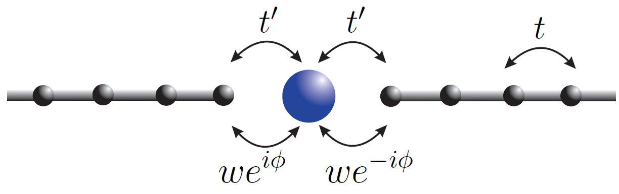
Figure 1: Schematic representation of the Anderson model with $\mathcal{PT}$-symmetric non-Hermitian hopping between the quantum dot and the wires.

The Hamiltonian in Eq. (1) can be mapped to a Kondo model in the regime $t^{\prime},w\ll|\epsilon_{d}|,U$ Hewson (1993). In this case, we consider that in the low-energy subspace the localized state is occupied by a single electron with spin $\uparrow$ or $\downarrow$ (such that $n_{d}=\sum_{\sigma}n_{d\sigma}=1$). The Schrieffer-Wolff transformation generates an effective spin exchange interaction in the low-energy subspace by projecting out the high-energy states with $n_{d}=0$ or $n_{d}=2$. To second-order perturbation theory, we obtain the effective Hamiltonian $H_{\rm eff}=H_{0}+H_{I}$, where the Kondo interaction $H_{I}$ has the form

$$H_{I} = J_{0}\,{\displaystyle\left(c_{1}^{\dagger}+c_{-1}^{\dagger}\right)\frac{\boldsymbol{\sigma}}{2}\left(c^{\phantom{\dagger}}_{1}+c^{\phantom{\dagger}}_{-1}\right)\cdotp\mathbf{S}}$$ (8)

$${\displaystyle-iJ_{1}\left(c_{-1}^{\dagger}\frac{\boldsymbol{\sigma}}{2}c^{\phantom{\dagger}}_{-1}-c_{1}^{\dagger}\frac{\boldsymbol{\sigma}}{2}c_{1}\right)\cdotp\mathbf{S}}$$

$$-J_{2}\left(c_{1}^{\dagger}\frac{\boldsymbol{\sigma}}{2}c_{1}+c_{-1}^{\dagger}\frac{\boldsymbol{\sigma}}{2}c^{\phantom{\dagger}}_{-1}\right)\cdotp\mathbf{S}.$$

Here $\boldsymbol{\sigma}$ denotes the vector of Pauli matrices and $\mathbf{S}$ is the spin-$1/2$ operator of the localized electron. The exchange coupling constants are given by

$$J_{0} = J+J^{\prime}+2\sqrt{JJ^{\prime}}\cos\phi,$$ (9)

$$J_{1} = 2\sqrt{JJ^{\prime}}\sin\phi+J^{\prime}\sin\left(2\phi\right),$$ (10)

$$J_{2} = J^{\prime}\,\left[1-\cos\left(2\phi\right)\right],$$ (11)

where

$$J = 2{t^{\prime}}^{2}\left(\frac{1}{-\epsilon_{d}}+\frac{1}{U+\epsilon_{d}}\right)\ ,$$ (12)

$$J^{\prime} = 2{w}^{2}\left(\frac{1}{-\epsilon_{d}}+\frac{1}{U+\epsilon_{d}}\right)\ .$$ (13)

Note that $J_{0},J_{2}\geq 0$. The first term in Eq. (8) corresponds to the standard antiferromagnetic Kondo coupling between the impurity spin and the symmetric orbital on sites $j=1$ and $j=-1$ of the wires Simon and Affleck (2001). This is the only coupling that survives in the Hermitian case $\phi=0,\pi$. By contrast, $J_{2}$ represents a ferromagnetic two-channel Kondo coupling Nozières, Ph. and Blandin, A. (1980); Zawadowski (1980) between the impurity and the spins at the ends of the wires. Finally, $J_{1}$ is the coupling constant of the non-Hermitian term. This term is odd under both $\mathcal{P}$ and $\mathcal{T}$ (with $\mathcal{T}:\mathbf{S}\mapsto-\mathbf{S}$ for the impurity spin), thus preserving the $\mathcal{PT}$ symmetry of the original model in Eq. (1).

III Renormalization Group

The Kondo effect can be understood within a perturbative RG analysis Anderson (1970); Hewson (1993); Affleck (1995). First, let us recall the result for the conventional Kondo model for an embedded quantum dot, which corresponds to setting $J_{1}=J_{2}=0$ in Eq. (8). In the RG analysis, the constant $J_{0}$ must be replaced by an effective interaction $J_{0}(\Lambda)$ that depends on the energy scale $\Lambda$ at which the properties of the system are measured. In the low-energy limit, $\Lambda\to 0$, the effective interaction diverges. The interpretation is that the localized spin forms a singlet with an electron in the symmetric channel between the two wires. The low-energy physics is described by a Fermi liquid fixed point Nozières (1974) at which the boundary conditions on conduction electrons are modified by a universal phase shift (in the case of particle-hole symmetry), leading to an ideal conductance between the two wires Glazman and Pustilnik (2003).

We now consider the $\mathcal{PT}$-symmetric Kondo model in the weak coupling regime $J_{0},J_{1},J_{2}\ll t$. For $J_{0}=J_{1}=J_{2}=0$, the Hamiltonian in Eq. (8) describes two decoupled tight-binding models with open boundary conditions at $j=0$. This free Hamiltonian can be diagonalized using the Fourier transform

$$c_{j<0}=\int_{0}^{\pi}\frac{dk}{\pi}\sin(kj)c_{k1},$$ (14)

$$c_{j>0}=\int_{0}^{\pi}\frac{dk}{\pi}\sin(kj)c_{k2},$$ (15)

where $c_{k\eta}$, with $\eta=1,2$, are the annihilation operators of electrons with momentum $k$ in the wire on the left for $\eta=1$ or on the right for $\eta=2$. The operators $c_{k\eta}$ obey $\{c^{\phantom{\dagger}}_{k\eta},c^{\dagger}_{k^{\prime}\eta^{\prime}}\}=2\pi\delta_{\eta\eta^{\prime}}\delta(k-k^{\prime})$. We can then write

$$H_{0}=\sum_{\eta=1,2}\int_{0}^{\pi}\frac{dk}{2\pi}\varepsilon(k)c^{\dagger}_{k\eta}c^{\phantom{\dagger}}_{k\eta},$$ (16)

where $\varepsilon(k)=-2t\cos(k)$ is the dispersion relation. At half-filling (the particle-hole symmetric case), the ground state is constructed by occupying the single-particle states with $0<k<k_{F}=\pi/2$. We take the continuum limit by linearizing the spectrum around the Fermi point. In real space, the operators $c_{j}$ are replaced by the fields $\psi_{\eta}(x)$ in the form Simon and Affleck (2001)

$$c_{j<0}\rightarrow\psi_{1}(x=j)\sim e^{ik_{F}x}\psi_{R1}(x)+e^{-ik_{F}x}\psi_{L1}(x),$$

$$c_{j>0}\rightarrow\psi_{2}(x=j)\sim e^{ik_{F}x}\psi_{R2}(x)+e^{-ik_{F}x}\psi_{L2}(x).$$ (17)

Here $\psi_{R/L,\eta}(x)$ are the slowly varying right- or left-moving components of the fermionic field, respectively. We impose open boundary conditions, $\psi_{\eta}(0)=0$, by the relation

$$\psi_{L\eta}(x)=-\psi_{R\eta}(-x).$$ (18)

Thus, the left movers in wire $\eta=1$ (the outgoing modes with respect to scattering at the boundary) can be regarded as the analytic continuation of the right movers to the positive-$x$ axis (see Fig. 2). Likewise, we treat the right movers in wire $\eta=2$ as the analytic continuation of the left movers. Defining the four-component spinor

$$\Psi(x)=\left(\begin{array}[]{cc}\psi_{L2}(-x)\\ \psi_{R1}(x)\end{array}\right)=\left(\begin{array}[]{cccc}\psi_{L2\uparrow}(-x)\\ \psi_{L2\downarrow}(-x)\\ \psi_{R1\uparrow}(x)\\ \psi_{R1\downarrow}(x)\end{array}\right),$$ (25)

we can write the free Hamiltonian in the low-energy approximation as

$$H_{0} \approx v_{F}\int_{-\infty}^{+\infty}dx\Psi^{\dagger}(x)(-i\partial_{x})\Psi(x),$$ (26)

where $v_{F}=2t\sin(k_{F})$ is the Fermi velocity.

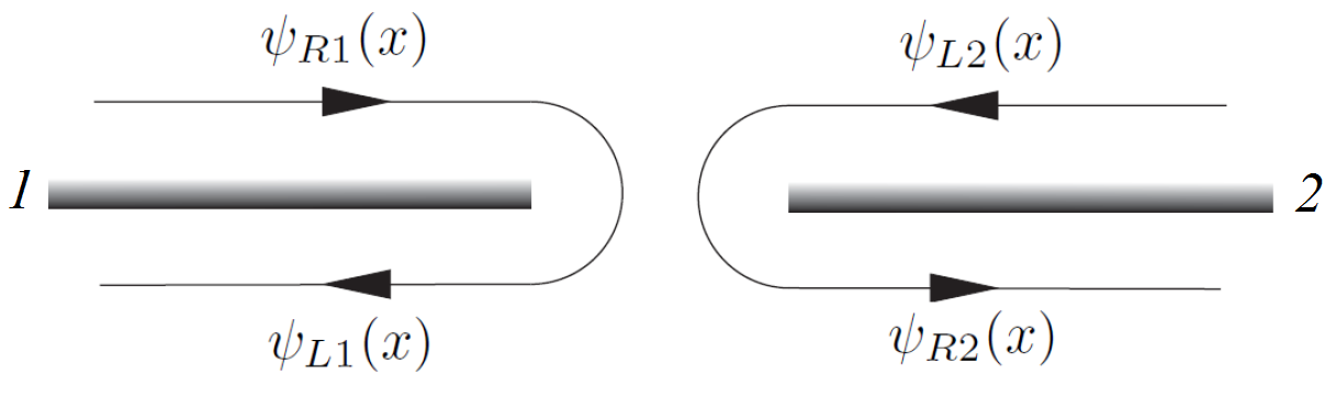
Figure 2: Low-energy modes for electrons in the two wires with open boundary conditions at $x=0$.

We now rewrite the interacting part of the Hamiltonian in the continuum limit using Eqs. (17) and (18) with $\psi_{R/L,\eta}(\pm 1)\approx\psi_{R/L,\eta}(0)$. The result is

$$H_{I}\approx\pi v_{F}\Psi^{\dagger}(0)\left(\lambda_{0}\boldsymbol{\Sigma}+i\lambda_{1}\boldsymbol{\Omega}-\lambda_{2}\boldsymbol{\Gamma}\right)\Psi(0)\cdot\mathbf{S},$$ (27)

where $\displaystyle\lambda_{n}=J_{n}\sin(k_{F})/(\pi t)$ with $n=0,1,2$ are the dimensionless Kondo couplings and the $4\times 4$ matrices $\boldsymbol{\Sigma}$, $\boldsymbol{\Omega}$ and $\boldsymbol{\Gamma}$ are written in terms of the Pauli matrices as follows:

$$\boldsymbol{\Sigma}=\left(\begin{array}[]{cc}\boldsymbol{\sigma}&\boldsymbol{\sigma}\\ \boldsymbol{\sigma}&\boldsymbol{\sigma}\end{array}\right),\,\boldsymbol{\Omega}=\left(\begin{array}[]{cc}\boldsymbol{\sigma}&0\\ 0&-\boldsymbol{\sigma}\end{array}\right),\,\boldsymbol{\Gamma}=\left(\begin{array}[]{cc}\boldsymbol{\sigma}&0\\ 0&\boldsymbol{\sigma}\end{array}\right).$$ (34)

These matrices obey the algebra

$$\left[\Sigma^{a},\Sigma^{b}\right] = 2\left[\Sigma^{a},\Gamma^{b}\right]=2\left[\Gamma^{a},\Sigma^{b}\right]=4i\epsilon^{abc}\Sigma^{c},$$

$$\left[\Gamma^{a},\Gamma^{b}\right] = \left[\Omega^{a},\Omega^{b}\right]=2i\epsilon^{abc}\Gamma^{c},$$

$$\left[\Omega^{a},\Gamma^{b}\right] = 2i\epsilon^{abc}\Omega^{c},$$

$$\left[\Omega^{a},\Sigma^{b}\right] = 2i\epsilon^{abc}\Omega^{c}+2i\delta^{ab}\Upsilon,$$ (35)

where $\Upsilon=\left(\begin{array}[]{cc}0&-i\mathbb{I}_{2}\\ i\mathbb{I}_{2}&0\end{array}\right)$ and $\mathbb{I}_{2}$ is the $2\times 2$ identity matrix. Equation (27) contains the most general boundary exchange interactions allowed by (spin-rotation) SU(2) and $\mathcal{PT}$ symmetries.

We calculate the RG equations using perturbation theory to second order in couplings $\lambda_{0}$, $\lambda_{1}$ and $\lambda_{2}$ following the procedure for the Kondo model Affleck (1995). In this calculation, we employ the algebra in Eq. (III). We also use the time-ordered matrix Green’s function for free electrons

$$G(t-t^{\prime}) = -i\left\langle T\Psi(0,t)\Psi^{\dagger}(0,t^{\prime})\right\rangle$$ (36)

$$= -\frac{\mathbb{I}_{4}}{2\pi v_{F}(t-t^{\prime})},$$

where $\mathbb{I}_{4}$ is the $4\times 4$ identity matrix. In the RG step, we integrate out short time intervals between scattering processes, $\Lambda^{-1}<|t-t^{\prime}|<(\Lambda^{\prime})^{-1}$, where $\Lambda$ and $\Lambda^{\prime}=\Lambda-d\Lambda$ are the old and new high-energy cutoff scales, respectively. We obtain the followings set of RG equations:

$$\frac{d\lambda_{0}}{d\ell} = \lambda_{0}^{2}-\lambda_{0}\lambda_{2}\ ,$$ (37)

$$\frac{d\lambda_{1}}{d\ell} = \lambda_{0}\lambda_{1}-\lambda_{1}\lambda_{2}\ ,$$ (38)

$$\frac{d\lambda_{2}}{d\ell} = -\frac{\lambda_{2}^{2}}{2}+\frac{\lambda_{1}^{2}}{2},$$ (39)

where $d\ell=d\Lambda/\Lambda$. At first sight, these RG equations involve three independent couplings, generating a three-dimensional flow diagram. However, by combining Eqs. (37) and (38), one can verify that the ratio

$$g\equiv\frac{\lambda_{1}}{\lambda_{0}}$$ (40)

is conserved along the RG flow, i.e., $dg/d\ell=0$, at least for the beta functions calculated to second order in the couplings. Substituting $J_{1}=gJ_{0}$, we are left with only two coupled RG equations:

$$\frac{d\lambda_{0}}{d\ell} = \lambda_{0}^{2}-\lambda_{0}\lambda_{2},$$ (41)

$$\frac{d\lambda_{2}}{d\ell} = -\frac{{\lambda}_{2}^{2}}{2}+g^{2}\frac{\lambda_{0}^{2}}{2}.$$ (42)

Figure 3 shows the RG flow according to Eqs. (41) and (42) for different values of $g$. Fig. 3(a) corresponds to the Hermitian case $g=0$. Along the line $\lambda_{2}=0$, we recover the usual Kondo effect Hewson (1993): the dimensionless Kondo coupling $\lambda_{0}$ is marginally irrelevant in the ferromagnetic case $\lambda_{0}<0$ and marginally relevant in the antiferromagnetic case $\lambda_{0}>0$. In the regime $0<\lambda_{2}<\lambda_{0}$, we have $\lambda_{0}(\Lambda)\to\infty$ while $\lambda_{2}(\Lambda)\to 0$ as $\Lambda\to 0$. When we turn on $g\neq 0$, as in Fig. 3(b), the flow to strong coupling is no longer along the $\lambda_{2}=0$ line because $\lambda_{2}$ grows together with $\lambda_{0}$. This suggests that the presence of the non-Hermitian term affects the asymptotic value of the ratio $\lambda_{2}/\lambda_{0}$ in the low-energy limit. Figure 3(c) shows that $|g|=1$ is a critical value, characterized by a discontinuity of the flow across the line $\lambda_{2}=\lambda_{0}$. For $|g|>1$, as in Fig. 3(d), the flow becomes non-monotonic: for $0<\lambda_{2}<\lambda_{0}$, the couplings initially increase, but eventually turn around and flow back to the non-interacting fixed point $\lambda_{0}=\lambda_{2}=0$, regardless of their initial values. Similar unconventional behavior is observed in the renormalization of the interactions of the non-Hermitian sine-Gordon model in the $\mathcal{PT}$-broken phase Ashida et al. (2017).

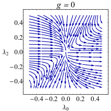
(a)

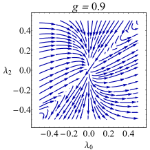
(b)

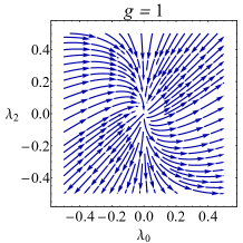
(c)

(d)

Figure 3: RG flow diagrams for the couplings $\lambda_{0}$ and $\lambda_{2}$ and different values of $g$: (a) $g=0$, (b) $g=0.9$, (c) $g=1$, and (d) $g=1.1$.

IV Spectrum in the strong coupling limit

We saw in Sec. III that, for $|g|<1$ and depending on the bare values of $\lambda_{0},\lambda_{2}>0$, the system can flow to strong coupling in the low-energy limit. As in the usual Kondo effect, we can understand the strong-coupling fixed point by going back to the lattice model and analyzing the limit in which the interactions are dominant, $J_{0},J_{2}\gg t$ Simon and Affleck (2001). In this limit, we start by diagonalizing $H_{I}$ in Eq. (8). The latter can be viewed as a three-site operator that acts in the Hilbert space $\mathcal{H}=\mathcal{H}_{-1}\otimes\mathcal{H}_{0}\otimes\mathcal{H}_{1}$, where $\mathcal{H}_{\pm 1}=\{|0\rangle,|\uparrow\rangle,|\downarrow\rangle,|\uparrow\downarrow\rangle,\}$ are the local Hilbert spaces of electrons in sites $j=\pm 1$ and $\mathcal{H}_{0}=\{|\Uparrow\rangle,|\Downarrow\rangle\}$ is the Hilbert space of the impurity spin.

We can block diagonalize the Kondo interaction $H_{I}$ in sectors labeled by the total number of electrons $N_{e}=c^{\dagger}_{-1}c^{\phantom{\dagger}}_{-1}+c^{\dagger}_{1}c^{\phantom{\dagger}}_{1}$ and by one component of the total spin $S^{z}_{\text{tot}}=c^{\dagger}_{-1}\frac{\sigma^{z}}{2}c^{\phantom{\dagger}}_{-1}+S^{z}+c^{\dagger}_{1}\frac{\sigma^{z}}{2}c^{\phantom{\dagger}}_{1}$. The possible values for these good quantum numbers are $N_{e}=0,1,\dots,4$ and $-(\tilde{N}_{e}+1)/2\leq S^{z}_{\text{tot}}\leq(\tilde{N}_{e}+1)/2$, where $\tilde{N}_{e}=\text{min}\{N_{e},4-N_{e}\}$. We also have the selection rule that $S^{z}_{\text{tot}}$ is integer if $N_{e}$ is odd and half-integer if $N_{e}$ is even. Due to particle-hole symmetry, the spectrum for $N_{e}=n$ electrons is the same as for $N_{e}=4-n$ electrons. Thus, we can restrict ourselves to $0\leq N_{e}\leq 2$. Likewise, due to SU(2) symmetry, the spectrum for spin $S^{z}_{\text{tot}}=m$ is the same as for $S^{z}_{\text{tot}}=-m$ and we focus on $m\geq 0$.

Let us denote the energy levels in each subspace by $E_{l}(N_{e},S^{z}_{\text{tot}})$, where $l$ runs from $l=1$ to the dimension of the subspace. In the sector with $N_{e}=0$, the interacting Hamiltonian $H_{I}$ vanishes identically, thus $E_{l}(0,1/2)=0$, with $l=1,2$. For $N_{e}=1$ and $S^{z}_{\text{tot}}=1$, we find two energy levels given by

$$E_{1,2}(1,1)=\frac{1}{4}\left(J_{0}-J_{2}\pm J_{0}\sqrt{1-g^{2}}\right).$$ (43)

Note that these energies are real for $|g|\leq 1$. For $|g|>1$, $E_{1,2}(1,1)$ form a complex conjugate pair. This corresponds to the spontaneous breaking of $\mathcal{PT}$ symmetry and it is a first sign that $g=\pm 1$ are exceptional points of the Kondo interactions. We confirm this expectation by calculating the energy levels in the other sectors. For $N_{e}=1$ and $S^{z}_{\text{tot}}=0$, the eigenvalues are

$$E_{1,2}(1,0) = -\frac{3}{4}\left(J_{0}-J_{2}\pm J_{0}\sqrt{1-g^{2}}\right),$$ (44)

$$E_{3,4}(1,0) = \frac{1}{4}\left(J_{0}-J_{2}\pm J_{0}\sqrt{1-g^{2}}\right).$$ (45)

Once again, the energies are real for $|g|\leq 1$. Here $E_{1}(1,0)$ and $E_{2}(1,0)$ are associated with singlet states (i.e., eigenstates of $\mathbf{S}_{\text{tot}}^{2}$ with $S_{\text{tot}}=0$). Their wave functions are antisymmetric in the spin part, but they correspond to different orbital states. For $|g|<1$, the singlet state with the lowest energy, $E_{1}(1,0)$, has the form

$$|\Psi_{0}\rangle=\frac{1}{2}\left[\left|\uparrow,\Downarrow,0\right\rangle-\left|\downarrow,\Uparrow,0\right\rangle+e^{i\alpha}\left(\left|0,\Downarrow,\uparrow\right\rangle-\left|0,\Uparrow,\downarrow\right\rangle\right)\right],$$ (46)

where $\alpha=\text{arctan}(g/\sqrt{1-g^{2}})$. Note that $|\Psi_{0}\rangle$ is an eigenstate of $\mathcal{PT}$ and for $g=0$ it reduces to the singlet state in the symmetric orbital, where the electron is in the superposition $(|j=-1\rangle+|j=1\rangle)/\sqrt{2}$.

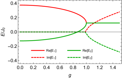
Figure 4: Real and imaginary parts of the energies in the sector with $N_{e}=1$ and $S^{z}_{\text{tot}}=1$ as given in Eq. (43). Here we set $J_{2}=J_{0}/2$. The spectrum becomes complex for $|g|>1$.

For $N_{e}=2$ and $S^{z}_{\text{tot}}=3/2$, we have only one state (${|\uparrow,\Uparrow,\uparrow\rangle}$) with energy $E_{1}(2,3/2)=(J_{0}-J_{2})/2$, independent of the parameter $g$. Finally, for $N_{e}=2$ and $S^{z}_{\text{tot}}=1/2$, we have five energy levels: $E_{1}(2,1/2)=E_{2}(2,1/2)=0$, $E_{3}(2,1/2)=(J_{0}-J_{2})/2$, and

$$E_{4,5}(2,1/2) = -\frac{J_{0}-J_{2}}{2}$$ (47)

$$\pm\frac{1}{2}\sqrt{3J_{0}(1-g^{2})+(J_{0}-J_{2})^{2}}.$$

The latter pair of eigenvalues becomes complex for $|g|>\sqrt{1+(1-J_{2}/J_{0})^{2}/3}\geq 1$. Therefore, for $|g|<1$ the entire spectrum of $H_{I}$ is real and the $\mathcal{PT}$ symmetry is preserved. For $|g|>1$, at least the eigenvalues in the $N_{e}=1$ sector become complex and the $\mathcal{PT}$ symmetry is spontaneously broken.

Figure 4 illustrates the behavior of the energy levels $E_{l}(1,1)$ as a function of $g$. As we approach $g=1$ from below, the eigenvalues coalesce with the characteristic square-root dependence of exceptional points Heiss (2012). For $|g|=1$, the eigenvalues of $H_{I}$ depend only on the difference $J_{0}-J_{2}$. In particular, for $J_{0}=J_{2}$, all the eigenstates become degenerate with eigenvalue zero, implying that the impurity effectively decouples from the wires. Note that the condition $|g|=1$ and $J_{0}=J_{2}$ also corresponds to the special line (a separatrix) $\lambda_{0}=\lambda_{1}=\lambda_{2}$ in the weak-coupling RG flow shown in Fig. 3(c).

V Strong-coupling fixed point and conductance

When the effective Kondo couplings diverge in the low-energy limit, ${J_{n}(\Lambda)\to\infty}$ with $J_{0}(\Lambda)>J_{2}(\Lambda)$ along the flow, a conduction electron forms a singlet with the impurity spin. The low-energy effective Hamiltonian for the remaining electrons in the wires can be obtained by projecting out the $\mathcal{PT}$-symmetric orbital involved in the singlet state in Eq. (46). We introduce the linear combinations

$$\tilde{c}_{\pm,\sigma}=\frac{1}{\sqrt{2}}\left(c_{-1,\sigma}\pm e^{-i\alpha}c_{1,\sigma}\right).$$ (48)

For $\alpha=0$, these are the annihilation operators for symmetric and antisymmetric orbitals (which are eigenstates of $\mathcal{P}$), respectively. In the more general $\mathcal{PT}$-symmetric problem, $c_{+,\sigma}$ annihilates an electron with spin $\sigma$ in the orbital state that becomes inaccessible at low energies where the singlet cannot be broken. We then define the projection operator $P$ onto the remaining electronic orbitals, such that $Pc_{-1}P=\tilde{c}_{-}/\sqrt{2}$ and $Pc_{1}P=-e^{i\alpha}\tilde{c}_{-}/\sqrt{2}$. The projection of the tight-binding Hamiltonian in the wires gives

$$H_{\text{sc}} = PH_{0}P$$ (49)

$$= -t{\displaystyle\sum_{j\leq-3}\left(c_{j}^{\dagger}c^{\phantom{\dagger}}_{j+1}+\text{h.c.}\right)}-t{\displaystyle\sum_{j\geq 2}\left(c_{j}^{\dagger}c^{\phantom{\dagger}}_{j+1}+\text{h.c.}\right)}$$

$$-\frac{t}{\sqrt{2}}\left(c^{\dagger}_{-2}\tilde{c}^{\phantom{\dagger}}_{-}-e^{i\alpha}c^{\dagger}_{2}\tilde{c}_{-}+\text{h.c.}\right).$$

Note that the magnitude of hopping parameter is reduced by a factor of $1/\sqrt{2}$ at the junction. Moreover, there is a phase factor $e^{i(\alpha+\pi)}$ associated with the (Hermitian) hopping process between the state annihilated by $\tilde{c}_{-}$ and the site $j=2$. This phase factor can be removed by performing the gauge transformation $c_{j}\to-e^{i\alpha}c_{j}$ for ${j\geq 2}$. We then obtain

$$\tilde{H}_{\text{sc}} = -t{\displaystyle\sum_{j\leq-3}\left(c_{j}^{\dagger}c^{\phantom{\dagger}}_{j+1}+\text{h.c.}\right)}-t{\displaystyle\sum_{j\geq 2}\left(c_{j}^{\dagger}c^{\phantom{\dagger}}_{j+1}+\text{h.c.}\right)}$$ (50)

$$-\frac{t}{\sqrt{2}}\left(c^{\dagger}_{-2}\tilde{c}^{\phantom{\dagger}}_{-}+c^{\dagger}_{2}\tilde{c}_{-}+\text{h.c.}\right).$$

This is now a $\mathcal{P}$- and $\mathcal{T}$-invariant tight-binding model for a single infinite wire. Remarkably, it coincides with the effective Hamiltonian for the usual Kondo model in the strong coupling limit Simon and Affleck (2001).

The linear conductance $G$ can be related to the transmission amplitude $T$ through the junction using the Landauer-Büttiker formalism Datta (1997):

$$G=\frac{2e^{2}}{h}T.$$ (51)

At the strong coupling fixed point described by Hamiltonian (50), the transmission amplitude can be calculated by solving the single-particle scattering problem. Following Refs. Simon and Affleck (2001); Pustilnik and Glazman (2001), we obtain $T=\sin^{2}(k_{F})$ Simon and Affleck (2001), which implies ideal transmittance $T=1$ in the particle-hole symmetric case $k_{F}=\pi/2$. This leads to the ideal conductance $G=2e^{2}/h$ at the strong-coupling fixed point, as for the usual Kondo effect in quantum dots Pustilnik and Glazman (2004).

On the other hand, in the regime $|g|>1$, the effective couplings $\lambda_{n}(\Lambda)$, with $n=0,1,2$, vanish in the low-energy limit. In fact, it follows from the RG equations (41) and (42) that they vanish logarithmically, $\lambda_{n}(\Lambda)\sim[\ln(\Lambda_{0}/\Lambda)]^{-1}$ for $\Lambda\to 0$, where $\Lambda_{0}\sim t$ is the bare cutoff scale. The conductance in this case can be calculated similarly to the weak coupling regime of the Kondo model, namely by starting from the Kubo formula and applying second-order perturbation theory in the effective couplings (see Refs. Pustilnik and Glazman (2004); Ng and Lee (1988) for details). Therefore, in the $\mathcal{PT}$-broken regime $|g|>1$, the conductance scales as $G(\Lambda)\sim[\ln(\Lambda_{0}/\Lambda)]^{-2}$ and vanishes at the local-moment fixed point, at which the wires decouple from the impurity and the currents are totally reflected at the boundary.

Within the effective field theory, the strong-coupling fixed point can be understood as a $\pi/2$ phase shift that changes the boundary conditions of electron states in the channel involved in the Kondo coupling Affleck (1995). The effective field theory can also be used to show that the Kondo fixed point is stable. Since the impurity spin disappears from the low-energy effective Hamiltonian, the perturbations to the Kondo fixed point are all irrelevant boundary operators and the low-energy properties are described by a local Fermi liquid theory Nozières (1974). No relevant perturbations arise in the non-Hermitian model with $\mathcal{PT}$, SU(2) and particle-hole symmetries. Particle-hole symmetry breaking allows for marginal perturbations that reduce the conductance from the ideal to a lower non-universal value. In the Hermitian Kondo model, this marginal perturbation corresponds to the $s$-wave potential scattering term $V_{0}\Psi^{\dagger}(0)\Psi(0)$ Hewson (1993). In the non-Hermitian model without particle-hole symmetry, we have an additional marginal perturbation allowed by $\mathcal{PT}$ symmetry, represented by $V_{1}\Psi^{\dagger}(0)\Upsilon\Psi(0)$ (where $\Upsilon$ is the imaginary antisymmetric matrix in Eq. (III)).

Finally, we comment on the possibility of varying the parameter $g$ across the exceptional point $g=1$. Using the perturbative expressions for the bare exchange couplings in Eqs. (9)-(11), we can show that $g=\lambda_{1}/\lambda_{0}=J_{1}/J_{0}=\sin(2\theta)$ with

$$\theta=\arctan\left[\frac{\sqrt{JJ^{\prime}}\sin\phi}{J+\sqrt{JJ^{\prime}}\cos\phi}\right].$$ (52)

Therefore, these perturbative expressions predict $|g|\leq 1$. However, this relation does not hold beyond second-order perturbation theory in $t^{\prime}$ and $w$ or for a more general lattice model than Eq. (1) (for instance, including non-Hermitian hopping processes between the dot and the second site in each wire). More generally, the bare coupling constants $\lambda_{n}$ that set the initial values in the RG flow must be treated as independent phenomenological parameters. Nonetheless, the above result suggests that the spontaneous breaking of $\mathcal{PT}$ symmetry in our non-Hermitian Kondo model should be difficult to realize in the regime $t^{\prime},w\ll|\epsilon_{d}|,U$. Instead, one should look for stronger tunnelling between the wires and the quantum dot, but still in the Coulomb blockade regime where charge fluctuations in the dot can be neglected.

VI Conclusions

We have investigated an Anderson impurity model with $\mathcal{PT}$-symmetric non-Hermitian hopping between the wires and the localized state in the quantum dot. Using a Schrieffer-Wolff transformation, we obtained the $\mathcal{PT}$-symmetric Kondo model that describes the coupling to the impurity spin. Our perturbative renormalization group analysis showed that the fate of the Kondo effect is controlled by the parameter $g$ defined as the ratio between the non-Hermitian coupling and the usual single-channel Kondo coupling. For $|g|<1$, the spectrum of the Kondo interaction is real and the Kondo effect persists. In the particle-hole symmetric case, the strong coupling fixed point of the $\mathcal{PT}$-symmetric Kondo model has ideal conductance through the quantum dot. For $|g|>1$, the spectrum becomes complex and the $\mathcal{PT}$ symmetry is spontaneously broken. In this case, the low-energy physics is governed by a local-moment fixed point with zero conductance.

Some open questions include the generalization to the multichannel Kondo model Nozières, Ph. and Blandin, A. (1980); Affleck and Ludwig (1991) and the interplay of $\mathcal{PT}$-symmetric interactions at the boundary and in the bulk, as in the Kondo effect in Tomonaga-Luttinger liquids Lee and Toner (1992); Furusaki and Nagaosa (1994). More generally, it would be interesting to search for new boundary fixed points unique to $\mathcal{PT}$-symmetric non-Hermitian systems, perhaps with chiral transport properties analogous to those realized in quantum optics Lodahl et al. (2017); Longhi (2017). To go beyond perturbative approaches, it would be interesting to generalize powerful numerical techniques that have been instrumental in the study of quantum impurity models, such as Wilson’s numerical renormalization group Wilson (1975); Bulla et al. (2008).