VTrails: Inferring Vessels with Geodesic Connectivity Trees

Abstract

The analysis of vessel morphology and connectivity has an impact on a number of cardiovascular and neurovascular applications by providing patient-specific high-level quantitative features such as spatial location, direction and scale. In this paper we present an end-to-end approach to extract an acyclic vascular tree from angiographic data by solving a connectivity-enforcing anisotropic fast marching over a voxel-wise tensor field representing the orientation of the underlying vascular tree. The method is validated using synthetic and real vascular images. We compare VTrails against classical and state-of-the-art ridge detectors for tubular structures by assessing the connectedness of the vesselness map and inspecting the synthesized tensor field as proof of concept. VTrails performance is evaluated on images with different levels of degradation: we verify that the extracted vascular network is an acyclic graph (i.e. a tree), and we report the extraction accuracy, precision and recall.

1 Introduction

Vessel morphology and connectivity is of clinical relevance in cardiovascular and neurovascular applications. In clinical practice, the vascular network and its abnormalities are assessed by inspecting intensity projections, or image slices one at a time, or using multiple views of 3D rendering techniques. In a number of conditions, the connected vessel segmentation is required for intervention or treatment planning [18]. A schematic representation of the vascular network has an impact in interventional neuroradiology and in vascular surgery by providing patient-specific high-level quantitative features (spatial localization, direction and scale). In vascular image analysis these features are used for segmentation and labelling [13], with the final aim of reconstructing a physical vascular model for hemodynamic simulations, or catheter motion planning, or identifying (un)safe occlusion points [6]. With this view, previous studies addressed the problem of extracting a connected vascular network in a disjoint manner. First, [8, 12] proposed tubular enhancing methods in 3D with the aim of better contrasting vessels over a background: by using the eigendecomposition of either the Hessian matrix, or the image gradient projected on a unit sphere boundary, a scalar vesselness measure is obtained, which represents a vascular saliency map. Secondly, given the vascular saliency map, local disconnected branches or fragmented centerlines, [6, 11, 16] proposed a set of methods to recover a connected network: ‘cores’ identify and track furcating branches, whereas vascular graphs are recovered using minimum spanning tree algorithms on image-intensity features, or using graph kernels (subtree patterns) matched on a similarity metric. Alternatively, geometrical models embedding shape priors, or probabilistic models based on image-related features were employed to recover the connected vessel centerlines and prune artifacts from an initial set of segments. A different approach is proposed in [2], where the connected centerlines are recovered a-posteriori as medial axes of the 3D surface model which segments the lumen.
Given the varying complexity of the vascular network in healthy and diseased subjects and the lack of an extensive connected ground-truth for complex vascular networks of several anatomical compartments, the accurate and exhaustive extraction of the vessel connectivity remains however a challenging task.
Here we propose VTrails, a novel method that addresses vascular connectivity under a unified mathematical framework. VTrails enhances the connectedness of furcating, fragmented and tortuous vessels through scalar and high-order vascular features, which are employed in a greedy connectivity paradigm to determine the final vascular network. In particular, the vascular image is filtered first with a Steerable Laplacian of Gaussian Swirls filterbank, synthesizing simultaneously a connected vesselness map and an associated tensor field. Under the assumption that vessels join by minimal paths, VTrails then infers the unknown fully-connected vascular network as the minimal cost acyclic graph connecting automatically extracted seed nodes.

2 Methods

We introduce in section 2.1 a Steerable Laplacian of Gaussian Swirls (SLoGS) filterbank used to reconstruct simultaneously the vesselness map and the associated tensor field. The SLoGS filterbank is first defined, then a multiscale image filtering approach is described using a locally selective overlap-add method [15]. The connected vesselness map and the tensor field are integrated over scales.
In section 2.2, an anisotropic level-set combined with a connectivity paradigm extracts the fully-connected vascular tree using the synthesized connected vesselness map and tensor field.

Steerable Laplacian of Gaussian Swirls		Connected Vesselness and Tensor Field
$\Gamma(\mathbf{x},\boldsymbol{\sigma},\mathbf{c})$	$\Gamma_{\text{tube}}$	Multi-scale Pyramid
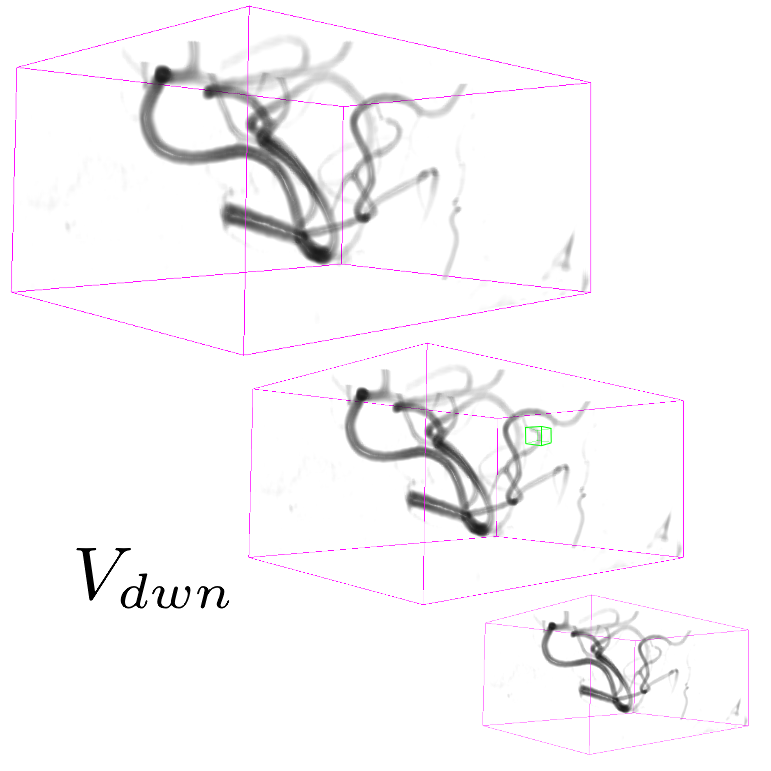
			TFs(b)
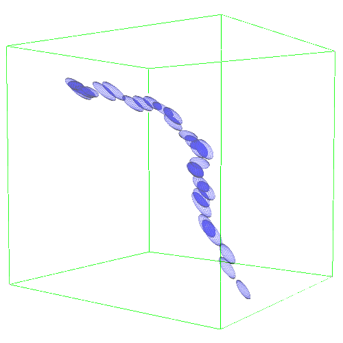
$K_{(\Gamma)}$ $T_{(\Gamma)}$	DFK

Figure 1: SLoGS filterbank: definition of a Dictionary of Filtering Kernels and synthesis of the Tensor Field within the overlap-add block $b$ at the given scale $s$.

2.1 SLoGS Curvilinear Filterbank

With the aim of enhancing the connectivity of fragmented, furcating and tortuous vessels, we propose a multi-resolution analysis/synthesis filterbank of Steerable Laplacian of Gaussian Swirls, whose elongated and curvilinear Gaussian kernels recover a smooth, connected and orientation aware vesselness map with local maxima at vessels’ mid-line.

2.1.1 Steerable Laplacian of Gaussian Swirls (SLoGS).

Similarly to [1] and without losing generality, given an image $V:\mathbb{R}^{3}\rightarrow\mathbb{R}$, the respective SLoGS vesselness response is obtained as $V_{SLoGS,s}:=V_{s}\ast K$, for any given scale $s$ and any predefined SLoGS filtering kernel $K\colon\mathbb{R}^{3}\rightarrow\mathbb{R}$. Here we formulate and derive the SLoGS filtering kernel $K$ by computing the second-order directional derivative in the gradient direction of a curvilinear Gaussian trivariate function $\Gamma\colon\mathbb{R}^{3}\times\mathbb{R}^{3}_{+}\times\mathbb{R}^{3}\rightarrow\mathbb{R}$. The gradient direction and its perpendicular constitute the first-order gauge coordinates system $(\boldsymbol{\omega},\boldsymbol{\upsilon})$. These are defined as $\boldsymbol{\omega}=\frac{\nabla\Gamma}{\|\nabla\Gamma\|}$, and $\boldsymbol{\upsilon}=\boldsymbol{\omega}_{\perp}$, with the spatial gradient $\nabla$. The function $\Gamma$ has the form

$${\Gamma\left(\mathbf{x},\boldsymbol{\sigma},\mathbf{c}\right)}=\frac{1}{\sqrt{2\pi\sigma_{1}^{2}}}e^{-\frac{x_{1}^{2}}{2\sigma_{1}^{2}}}\frac{1}{\sqrt{2\pi\sigma_{2}^{2}}}e^{-\frac{\left(x_{2}+c_{0}x_{1}+c_{1}x_{1}^{2}\right)^{2}}{2\sigma_{2}^{2}}}\frac{1}{\sqrt{2\pi\sigma_{3}^{2}}}e^{-\frac{\left(x_{3}+c_{2}x_{1}^{3}\right)^{2}}{2\sigma_{3}^{2}}}\enspace,$$ (1)

where $\mathbf{x}=x_{1}\underline{i}+x_{2}\underline{j}+x_{3}\underline{k}$, with $\{\underline{i},\underline{j},\underline{k}\}$ the Euclidean image reference system, $\boldsymbol{\sigma}$ modulates the elongation and the cross-sectional profiles of the Gaussian distribution, and the curvilinear factor $\mathbf{c}$ accounts for planar asymmetry and two levels of curvilinear properties (i.e. bending and tilting orthogonally to the elongation of the distribution) by means of quadratic- and cubic-wise bending of the support, respectively. For any $\boldsymbol{\sigma}$ and $\mathbf{c}$, $\Gamma\left(\mathbf{x},\boldsymbol{\sigma},\mathbf{c}\right)$ represents therefore the smooth impulse response of the Gaussian kernel. By operating a directional derivative on $\Gamma$ along $\boldsymbol{\omega}$, i.e. $\mathcal{D}_{\boldsymbol{\omega}}$, we obtain the SLoGS filtering kernel $K$ as

$${K}=\mathcal{D}_{\boldsymbol{\omega}}\left[\mathcal{D}_{\boldsymbol{\omega}}\Gamma\right]=\mathcal{D}_{\boldsymbol{\omega}}\left[\boldsymbol{\omega}^{t}\nabla\Gamma\right]\triangleq\boldsymbol{\omega}^{t}H\left(\Gamma\right)\boldsymbol{\omega},~{}\text{\small where}~{}H\left(\Gamma\right)=\begin{pmatrix}\Gamma_{\underline{i}\underline{i}}&\Gamma_{\underline{i}\underline{j}}&\Gamma_{\underline{i}\underline{k}}\\ \Gamma_{\underline{j}\underline{i}}&\Gamma_{\underline{j}\underline{j}}&\Gamma_{\underline{j}\underline{k}}\\ \Gamma_{\underline{k}\underline{i}}&\Gamma_{\underline{k}\underline{j}}&\Gamma_{\underline{k}\underline{k}}\end{pmatrix}$$ (2)

is the Hessian matrix of the Gaussian kernel. Given that $\Gamma$ is twice continuously differentiable, $H(\Gamma)$ is well defined. Since $H(\Gamma)$ is symmetric, an orthogonal matrix $Q$ exists, so that $H(\Gamma)$ can be diagonalized as $H(\Gamma)=Q\Lambda Q^{-1}$. The eigenvectors $\underline{q}_{l}$ form the columns of $Q$, whereas the eigenvalues $\lambda_{l}$, with $l=1,2,3$, constitute the diagonal elements of $\Lambda$, so that $\Lambda_{ll}=\lambda_{l}$ and $\|\lambda_{1}\|\leq\|\lambda_{2}\|\leq\|\lambda_{3}\|$. Given a point $\mathbf{x}$, $K(\mathbf{x})$ can be reformulated as $K(\mathbf{x})=\omega^{t}\left(Q\Lambda Q^{-1}\right)\omega$. Geometrically, the columns of $Q$ represent a rotated orthonormal basis in $\mathbb{R}^{3}$ relative to the image reference system so that $\underline{q}_{l}$ are aligned to the principal directions of $\Gamma$ at any given point $\mathbf{x}$. The diagonal matrix $\Lambda$ characterizes the topology of the hypersurface in the neighbourhood of $\mathbf{x}$ (e.g. flat area, ridge, valley or saddle point in 2D) and modulates accordingly the variation of slopes, being the eigenvalues $\lambda_{l}$ the second-order derivatives along the principal directions of $\Gamma$. Factorizing $K(\mathbf{x})$, we obtain: $K(\mathbf{x})=(\boldsymbol{\omega}^{t}Q)\Lambda(Q^{-1}\boldsymbol{\omega})$, so that the gradient direction $\boldsymbol{\omega}$ is mapped onto the principal directions of $\Gamma$ for any point $\mathbf{x}$. Solving (2)

$$\begin{split}{K(\mathbf{x})}&=\frac{1}{\Gamma_{\underline{i}}^{2}+\Gamma_{\underline{j}}^{2}+\Gamma_{\underline{k}}^{2}}\begin{pmatrix}\Gamma_{\underline{i}}\\ \Gamma_{\underline{j}}\\ \Gamma_{\underline{k}}\end{pmatrix}^{t}\overbrace{\underbrace{\begin{pmatrix}q_{11}&q_{21}&q_{31}\\ q_{12}&q_{22}&q_{32}\\ q_{13}&q_{23}&q_{33}\end{pmatrix}}_{Q}\underbrace{\begin{pmatrix}\lambda_{1}&0&0\\ 0&\lambda_{2}&0\\ 0&0&\lambda_{3}\end{pmatrix}}_{\Lambda}\underbrace{\begin{pmatrix}q_{11}&q_{12}&q_{13}\\ q_{21}&q_{22}&q_{23}\\ q_{31}&q_{32}&q_{33}\end{pmatrix}}_{Q^{-1}=Q^{t}}}^{H(\Gamma)}\begin{pmatrix}\Gamma_{\underline{i}}\\ \Gamma_{\underline{j}}\\ \Gamma_{\underline{k}}\end{pmatrix}=\\ &=\sum_{l=1}^{3}\gamma_{l}\lambda_{l}=\gamma_{1}\frac{\partial^{2}}{\partial\underline{q}\text{\textsubscript{1}}^{2}}\Gamma+\gamma_{2}\frac{\partial^{2}}{\partial\underline{q}\text{\textsubscript{2}}^{2}}\Gamma+\gamma_{3}\frac{\partial^{2}}{\partial\underline{q}\text{\textsubscript{3}}^{2}}\Gamma~{}\triangleq~{}\boldsymbol{\gamma}LoG(\Gamma)~{},~{}\text{\small where}\end{split}$$ (3)

$\gamma_{1}=\frac{(\Gamma_{\underline{i}}q_{11}+\Gamma_{\underline{j}}q_{12}+\Gamma_{\underline{k}}q_{13})^{2}}{\Gamma_{\underline{i}}^{2}+\Gamma_{\underline{j}}^{2}+\Gamma_{\underline{k}}^{2}}$, $\gamma_{2}=\frac{(\Gamma_{\underline{i}}q_{21}+\Gamma_{\underline{j}}q_{22}+\Gamma_{\underline{k}}q_{23})^{2}}{\Gamma_{\underline{i}}^{2}+\Gamma_{\underline{j}}^{2}+\Gamma_{\underline{k}}^{2}}$, and $\gamma_{3}=\frac{(\Gamma_{\underline{i}}q_{31}+\Gamma_{\underline{j}}q_{32}+\Gamma_{\underline{k}}q_{33})^{2}}{\Gamma_{\underline{i}}^{2}+\Gamma_{\underline{j}}^{2}+\Gamma_{\underline{k}}^{2}}$ modulate the respective components of the canonical Laplacian of Gaussian ($LoG$) filter oriented along the principal directions of $\Gamma$. It is clear that given any arbitrary orientation $\Omega$ as an orthonormal basis similar to $Q$, the proposed dictionary of filtering kernels can steer by computing the rotation transform, which maps the integral orientation basis of each Gaussian kernel $\Phi_{\Gamma}=\frac{\int(\Gamma(\mathbf{x})\cdot Q(\mathbf{x}))d\mathbf{x}}{\|\int(\Gamma(\mathbf{x})\cdot Q(\mathbf{x}))d\mathbf{x}\|}$ on $\Omega$. Together with the SLoGS filtering kernel $K$, we determine the second-moment matrix $T$ associated to the filter impulse response $\Gamma$ by adopting the ellipsoid model in the continuous neighborhood of $\mathbf{x}$. A symmetric tensor $T(\mathbf{x})$ is derived from the eigendecomposition of ${H(\Gamma)}$ as $T(\mathbf{x})=Q~{}\Psi~{}Q^{-1}$, where $\Psi$ is the diagonal matrix representing the canonical unitary volume ellipsoid

$${\Psi}={\left(\prod_{l=1}^{3}\psi_{l}\right)^{-\frac{1}{3}}}\left(\begin{smallmatrix}\psi_{1}&0&0\\ 0&\psi_{2}&0\\ 0&0&\psi_{3}\end{smallmatrix}\right),~{}~{}\text{\small being}~{}~{}\psi_{1}=\frac{|\lambda_{1}|}{\sqrt{|\lambda_{2}\lambda_{3}|}},~{}\psi_{2}=\frac{|\lambda_{2}|}{|\lambda_{3}|},~{}~{}\text{\small and}~{}~{}\psi_{3}=1$$ (4)

the respective semiaxes’ lengths. Conversely from $H(\Gamma)$, which is indeterminate, the tensor field $T$ is a symmetric positive definite (SPD) matrix for any $\mathbf{x}\in\mathbb{R}^{3}$. Here, the definition of the tensor kernel $T$ in (4) can be further reformulated exploiting the intrinsic log-concavity of $\Gamma$. By mapping $\Gamma\mapsto\tilde{\Gamma}=-\log(\Gamma)$, a convex quadratic form is obtained, so that $H(\tilde{\Gamma})$ is an SPD, as the modelled tensor $T$. In either case, the manifold of tensors can be mapped into a set of 6 independent components in the Log-Euclidean space, which greatly simplifies the computation of Riemannian metrics and statistics. We refer to [3] for a detailed methodological description. The continuous and smooth tensor field $T$ inherits the steerable property. Similarly to diffusion tensor MRI, the kernel shows a preferred diffusion direction for a given energy potential, e.g. the scalar function $\Gamma$ itself (fig. 1). This allows to define an arbitrary dictionary of filtering kernels (DFK) that embeds anisotropy and high-order directional features to scalar curvilinear templates, which enhances and locally resembles typical, smooth vessel patterns. Together with the arbitrary SLoGS DFK, we also introduce an extra pair of non-curvilinear kernels for completeness. These are the pseudo-impulsive $\delta LoG$, an isotropic derivative filter given by the Laplacian of Gaussian of $\Gamma_{\delta}(\mathbf{x},\boldsymbol{\sigma},\mathbf{c}=\mathbf{0})$, representing a Dirac delta function for $\boldsymbol{\sigma}\rightarrow 0$. Also, the uniformly flat $\nu LoG$ is another isotropic degenerate case, where the Laplacian of Gaussian derives from $\Gamma_{\nu}(\mathbf{x},\boldsymbol{\sigma},\mathbf{c}=\mathbf{0})$, which is assumed to be a uniform, constant-value kernel for $\boldsymbol{\sigma}\rightarrow\infty$. The purpose of introducing the extra kernels is to better contrast regions that most likely relate to vessel boundaries and to image background, respectively. Although $\delta LoG$ and $\nu LoG$ have singularities, ideally they represent isotropic degenerate kernels. Therefore we associate pure isotropic tensors for any given $\mathbf{x}\in\mathbb{R}^{3}$, so that $T_{\delta LoG}(\mathbf{x})=T_{\nu LoG}(\mathbf{x})=I_{3}$ (Identity). The respective directional kernel bases $\Phi(\delta LoG)=\Phi(\nu LoG)$ are undetermined.

2.1.2 Connected Vesselness Map and the Tensor Field.

The idea is to convolve finite impulse response SLoGS with the discrete vascular image in a scale- and rotation-invariant framework, to obtain simultaneously the connected vesselness maps and the associated tensor field. For simplicity, the filtering steps will be presented for a generic scale $s$. Scale-invariance is achieved by keeping the size of the small compact-support SLoGS fixed, while the size of the vascular image $V$ varies accordingly with the multi-resolution pyramid. Also, different $\boldsymbol{\sigma}$ will produce SLoGS kernels with different spatial band-pass frequencies. $V$ is down-sampled at the arbitrary scale $s$ as proposed in [7] to obtain $V_{dwn}$. An early saliency map of tubular structures $V_{tube}$ is then determined as

$$V_{tube}=\sum_{\Omega}V_{tube}^{(\Omega)}~{},~{}~{}\text{\small where}~{}~{}V_{tube}^{(\Omega)}=\max\left(0,V_{dwn}\ast K_{tube}^{(\Omega)}\right).$$ (5)

$K_{tube}$ is derived from the discretized tubular kernel $\Gamma_{tube}(\mathbf{x},\sigma_{1}>\sigma_{2}=\sigma_{3},\mathbf{c}=\mathbf{0})$ (fig. 1), whereas $\Omega$ is defined as a group of orthonormal basis in $\mathbb{R}^{3}$, using an icosphere at arbitrary subdivision level $n$ to determine the orientation sampling in 3D. $V_{tube}$ is meant to provide an initial, coarse, although highly-sensitive set of saliency features in $V_{dwn}$: the vessel spatial locations and orientations. The identification of such features has two advantages; firstly it restricts the problem of the rotation-invariant filtering to an optimal complexity in 3D avoiding unnecessary convolutions; secondly it allows to use a locally selective overlap-add (OLA) [15] for the analysis/synthesis filtering. In detail, vessel spatial locations are mapped as voxel seeds $\tilde{S}$, and the associated set of orientations $\Theta$ forms a group of orthonormal basis in $\mathbb{R}^{3}$. We define $\tilde{S}$ as

$$\tilde{S}=\text{div}\left(\nabla V_{tube}\right)_{<0}~{}\wedge~{}\lambda_{1,2,3}^{V_{tube}}<0~{}\wedge~{}V_{tube}\geq Q_{p}(V_{tube}^{+})\enspace,$$ (6)

where $\text{div}\left(\nabla V_{tube}\right)$ is the divergence of $V_{tube}$’s gradient vector field, $\lambda_{1:3}^{V_{tube}}$ are the eigenvalue maps derived from the voxel-wise eigendecomposition of $H(V_{tube})$, and $Q_{p}(V_{tube}^{+})$ is the p^th quantile of the positive $V_{tube}$ samples’ pool. With $\tilde{S}$, the orientations $\Theta$ are automatically determined as the set of eigenvectors associated to $\lambda_{1:3}^{V_{tube}}$. The greater the intensity threshold $Q_{p}(V_{tube}^{+})$, the greater the image noise-floor rejection, the lower the number of seeds and the fewer the details extracted from $V_{tube}$. Also, the cardinality of $\tilde{S}$ and $\Theta$ is a trade-off for the convolutional complexity in each OLA filtering step. The analysis/synthesis filtering can be embedded in a fully parallel OLA, by considering an overlapping grid of 3D cubic blocks spanning the domain of $V_{dwn}$, and by processing each block $b$ so that at least one seed exists within it. The integral connected vesselness map $\text{{CVM}}_{s}^{(b)}$, for each block $b$ at any given scale $s$, has the form

$$\text{{CVM}}_{s}^{(b)}=\sum_{K\in DFK}\,\sum_{\theta\in\Theta^{(b)}}V_{\mathcal{S}}^{(b,K,\theta)},~{}~{}\text{\small where}~{}~{}V_{\mathcal{S}}^{(b,K,\theta)}=\max\left(0,\left(V_{dwn}^{(b)}\cdot\mathcal{H}\right)\ast K^{(\theta)}\right).$$ (7)

Here, $V_{\mathcal{S}}^{(b,K,\theta)}$ is the convolutional filter response given the considered SLoGS kernel. In detail, $V_{dwn}^{(b)}$ is the down-sampled image in $b$, $\mathcal{H}$ is the 3D OLA Hann weighting window, and $K^{(\theta)}$ is the steered filtering kernel along $\theta\in\Theta^{(b)}$, those being the seeds’ orientations in $b$. Note that in the discrete domain each voxel has a spatial indexed location $\mathbf{b}\in b$. The anisotropic tensor field $\text{{TF}}_{s}^{(b)}$ is synthesized and normalized in the Log-Euclidean space as the integral weighted-sweep of each steered tensor patch within the block $b$, and has the form

$$\begin{smallmatrix}{\text{{TF}}_{s,(LE)}^{(b)}}=\dfrac{1}{W}~{}~{}\cdot{{\sum}}_{K\in\left\{\begin{smallmatrix}\scriptscriptstyle DFK,\\ \scriptscriptstyle\delta LoG,\\ \scriptscriptstyle\nu LoG\end{smallmatrix}\right\}}~{}{\sum}_{\theta\in\Theta^{(b)}}\underbrace{\left({\sum}_{\lfloor\mathbf{b}\rceil\subset b}\overbrace{V_{\mathcal{S}}^{(\mathbf{b},K,\theta)}\cdot\Gamma_{(K)}^{(\theta)}\cdot\Xi}^{\text{\scriptsize weights}}\cdot\overbrace{T^{(\theta)}_{K,(LE)}}^{\text{\scriptsize patch}}\right)}_{\text{\scriptsize within-block patch sweep}},~{}~{}\text{\small so that}\\ {\det{\left(\text{{TF}}_{s}^{(b)}(\mathbf{b})\right)=\mathcal{H}(\mathbf{b})}},~{}~{}\text{\small and~{}}\,{W}=\left(\sum_{K\in\left\{\begin{smallmatrix}\scriptscriptstyle DFK,\\ \scriptscriptstyle\delta LoG,\\ \scriptscriptstyle\nu LoG\end{smallmatrix}\right\}}~{}\sum_{\theta\in\Theta^{(b)}}\sum_{\lfloor\mathbf{b}\rceil\subset b}V_{\mathcal{S}}^{(\mathbf{b},K,\theta)}\cdot\Gamma_{(K)}^{(\theta)}\cdot\Xi\right),\end{smallmatrix}$$ (8)

where $W$ is the integral normalizing weight-map accounting for all vessel, boundary and background components; $V_{\mathcal{S}}^{(\mathbf{b},K,\theta)}$ is the modulating SLoGS filter response at $\mathbf{b}$ as in (7); $\Gamma_{(K)}^{(\theta)}$ is the steered Gaussian impulse response associated to the kernel $K\in\left\{DFK,\delta Log,\nu LoG\right\}$; $\Xi$ is the Hann smoothing window in the neighbourhood $\lfloor\mathbf{b}\rceil$ centred at $\mathbf{b}$, and $T^{(\theta)}_{K,(LE)}$ is one of the 6 components of the discrete steered tensors patch $T$ in the Log-Euclidean space. Note that all 6 tensorial components are equally processed, and that the neighbourhood $\lfloor\mathbf{b}\rceil$ and the SLoGS tensors patch $T^{(\theta)}_{K,(LE)}$ have the same size. In (8), $\text{{TF}}_{s,(LE)}^{(b)}$ integrates also the isotropic contributions from vessel boundaries and background to better contrast the tubular structures’ anisotropy and to reduce synthetic artifacts surrounding the vessels (fig. 1). In particular, $\text{{TF}}_{s,(LE)}^{(b)}$ is averaged with an identically null tensor patch in the Log-Euclidean space in correspondence of boundaries and background, and $V_{\mathcal{S}}^{(\mathbf{b},K,\theta)}|_{\{\delta LoG,\nu LoG\}}$ is computed as in (7), where the image negative of $V_{dwn}^{(b)}$ is considered. Lastly, the connected vesselness maps and the associated synthetic tensor field are reconstructed by adding adjacent overlapping blocks in the OLA 3D grid for the given scale $s$.

2.1.3 Integration over Multiple Scales.

Each scale-dependent contribution is up-sampled and cumulatively integrated with a weighted sum

$$\begin{array}[]{lcl}\text{{CVM}}=\sum_{s}\frac{1}{s}\text{{CVM}}_{s},&\text{\small~{}~{}~{}and,~{}~{}~{}}&\text{{TF}}_{(LE)}=\frac{1}{\text{{CVM}}}\sum_{s}\left(\frac{1}{s}\text{{CVM}}_{s}\right)\cdot T_{s,(LE)}.\end{array}$$ (9)

Vesselness contributions are weighted here by the inverse of $s$, emphasizing responses at spatial low-frequencies. We further impose that the Euclidean TF has unitary determinant at each image voxel; for stability, the magnitude of the tensors is decoupled from the directional and anisotropic features throughout the whole multi-scale process, since tensors’ magnitude is expressed by CVM. Note that with the proposed method we do not aim at segmenting vessels by thresholding the resulting CVM, we rather provide a measure of vessels’ connectedness with maximal response at the centre of the vascular structures.

2.2 Vascular Tree of Geodesic Minimal Paths

Following the concepts first introduced in [4], we formulate an anisotropic front propagation algorithm that combined with an acyclic connectivity paradigm joins multiple sources $\tilde{S}\mapsto S$ propagating concurrently on a Riemannian speed potential $\mathcal{P}$. Since we want to extract geodesic minimal paths between points, we minimize an energy functional $\mathcal{U}(\mathbf{x})=\min_{\pi}\int_{\pi}\mathcal{P}\left(\pi(\mathbf{x}),\pi^{\prime}(\mathbf{x})\right)d\mathbf{x}$ for any possible path $\pi$ between two generic points along its geodesic length, so that $\|\nabla\mathcal{U}(\mathbf{x})\|=1$, and $\mathcal{U}(S)=0$. The solution to the Eikonal partial differential equation is given here by the anisotropic Fast Marching (aFM) algorithm [4], where front waves propagate from $S$ on $\mathcal{P}$, with $\mathcal{P}\left(\pi,\pi^{\prime}\right)=\sqrt{\pi^{\prime t}\cdot\mathcal{M}\cdot\pi^{\prime}}$ describing the infinitesimal distance along $\pi$, relative to the anisotropic tensor $\mathcal{M}$. In our case, $\mathcal{M}=\text{{TF}}$, and $\pi^{\prime}\propto\frac{1}{\text{{CVM}}}$. Note that the anisotropic propagation is a generalised version of the isotropic propagation medium, $\mathcal{M}\equiv I_{3}$. The acyclic connectivity paradigm is run until convergence together with the aFM to extract the vascular tree of multiple connected geodesics $\Pi$.

2.2.1 Anisotropic FM and Acyclic Connectivity Paradigm.

Geodesic paths are determined by back-tracing $\mathcal{U}$ when different regions collide. The connecting geodesic $\pi$ is extracted minimizing $\mathcal{U}$ at the collision grid-points. The aFM maps, i.e. $\mathcal{U}$; the Voronoi index map $\mathcal{V}$, representing the label associated to each propagating seed; and the Tag $\mathcal{T}$, representing the state of each grid-point (Front, Visited, Far), are then updated within the collided regions, so that these merge as one and the front is consistent with the unified resulting region. This is continued until all regions merge.

Initialization. The seeds $\tilde{S}$ are aligned towards the vessels’ mid-line with a constrained gradient descent, resulting in an initial set of sources $S$. All 26-connected components $\pi_{p}^{(S)}\in S$ initialize the aFM maps, i.e., $\mathcal{U}(\pi_{p}^{(S)})=0$, $\mathcal{V}(\pi_{p}^{(S)})=p$, $\mathcal{T}(\pi_{p}^{(S)})=\text{{Front}}$, and constitute also the initial geodesics $\pi_{p}^{(S)}\rightarrow\Pi$.

Fast Marching Step. The aFM maps are updated by following an informative propagation scheme. We refer to [4] for the 3D aFM step considering the 48 simplexes in the 26-neighbourhood of the Front grid-point with minimal $\mathcal{U}$.

Path Extraction. Collision is detected when Visited grid-points of different regions are adjacent. A connecting $\pi$ is determined by linking the back-traced minimal paths from the collision grid-points to their respective sources $\pi_{A},\pi_{B}\in\Pi$ with a gradient descent on $\mathcal{U}$ (fig. 2). The associated integral geodesic length $U_{\pi}=\int_{\pi_{A}}^{\pi_{B}}\mathcal{U}d\pi$ is computed and the connectivity in $\Pi$ is updated in the form of an adjacency list. Lastly, the grid-points of the extracted $\pi$ are further considered as path seeds in the updating scheme, since furcations can occur at any level of the connecting minimal paths.

Fast Updating Scheme. A nested aFM is run only in the union of the collided regions $(A\cup B)$ using a temporary independent layer of aFM maps, where $\tilde{\mathcal{U}}(\pi)=0$, $\tilde{\mathcal{T}}(\pi)=\text{{Front}}$, and $\tilde{\mathcal{T}}_{(\overline{A\cup B})}=\text{{Visited}}$. Ideally, the nested aFM is run until complete domain exploration, however, to speed up the process, the propagation domain is divided into the solved and unsolved sub-regions, and the update is focused on the latter $(A\cup B)^{\text{{{u}}}}$ (fig. 2). The boundary geodesic values of $(A\cup B)^{\text{{{u}}}}$ equal the geodesic distances $\mathcal{U}$ at the collision grid-points. Lastly, the aFM maps are updated as: $\mathcal{U}_{(A\cup B)^{\text{{{u}}}}}=\min\,\{\,\mathcal{U}_{(A\cup B)^{\text{{{u}}}}},\,\tilde{\mathcal{U}}_{(A\cup B)^{\text{{{u}}}}}\}$, $\mathcal{V}_{(A\cup B)}=\min\,\{\,\mathcal{V}_{A},\,\mathcal{V}_{B}\}$, and $\mathcal{T}_{(A\cup B)^{\text{{{u}}}}}=\tilde{\mathcal{T}}_{(A\cup B)^{\text{{{u}}}}}$.

Initialization		FM Steps	Collision, Path Extraction and Update						Convergence
$\tilde{S}$ Descent		…	$\Pi\leftarrow p_{~{}i}$		$\Pi\leftarrow p_{~{}i+1}$		$\Pi\leftarrow p_{~{}i+2}$		Stop Criterion
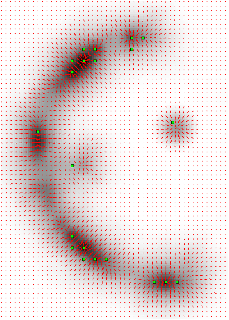
	$\mathcal{U}~{}\cup$ Trials
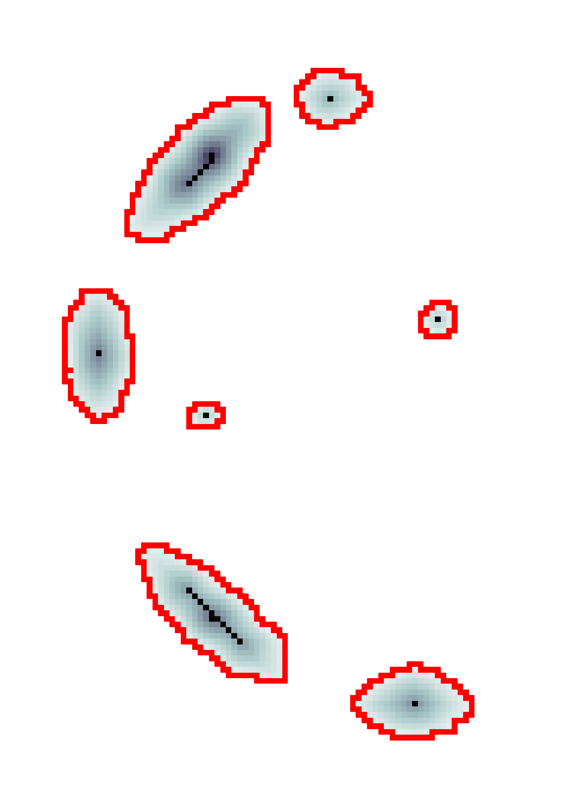
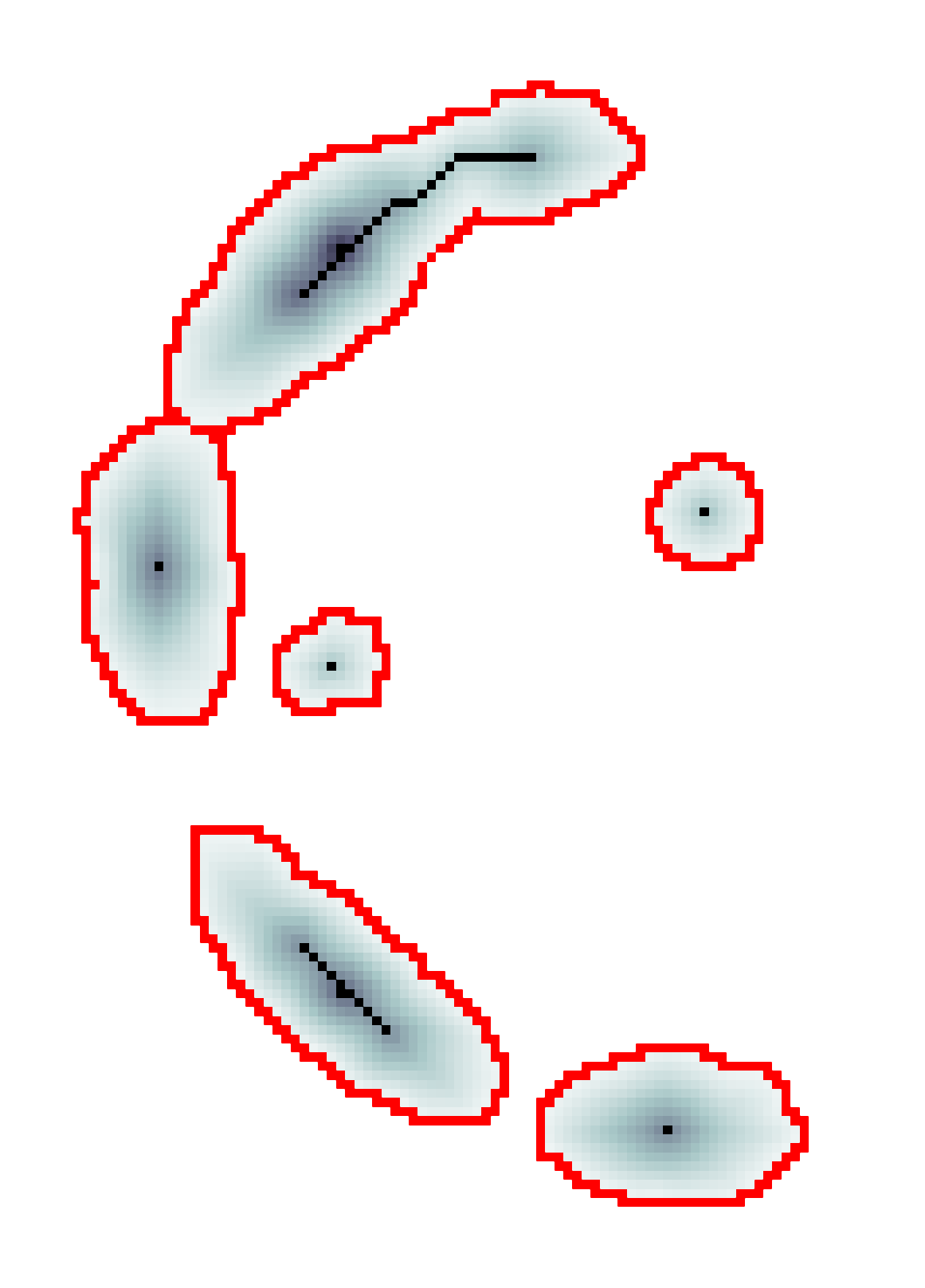
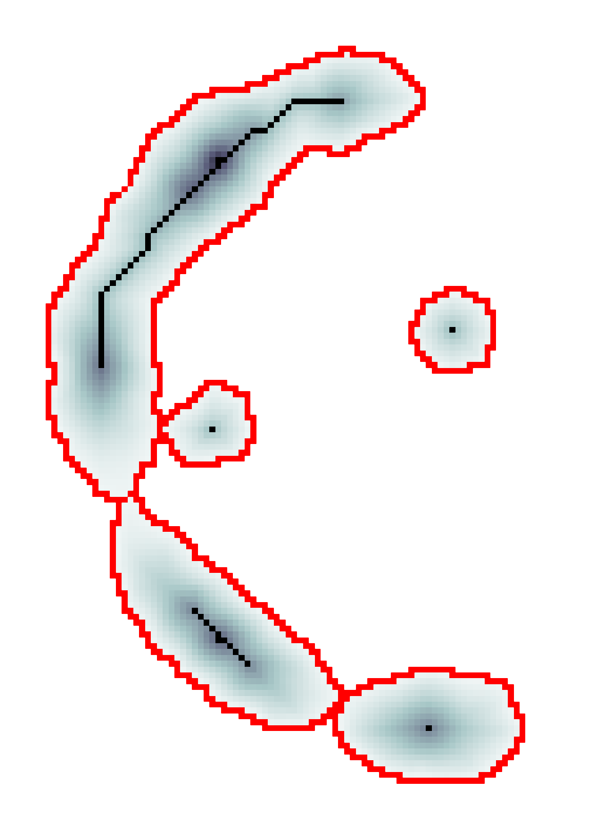
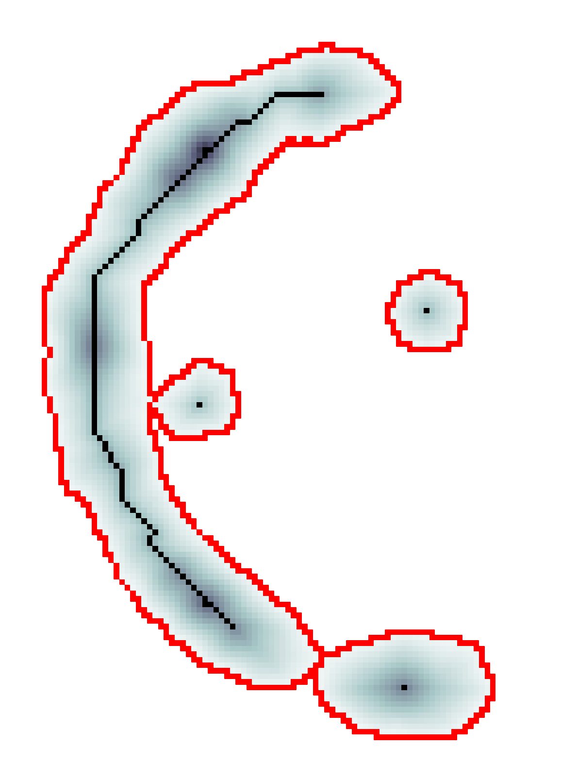
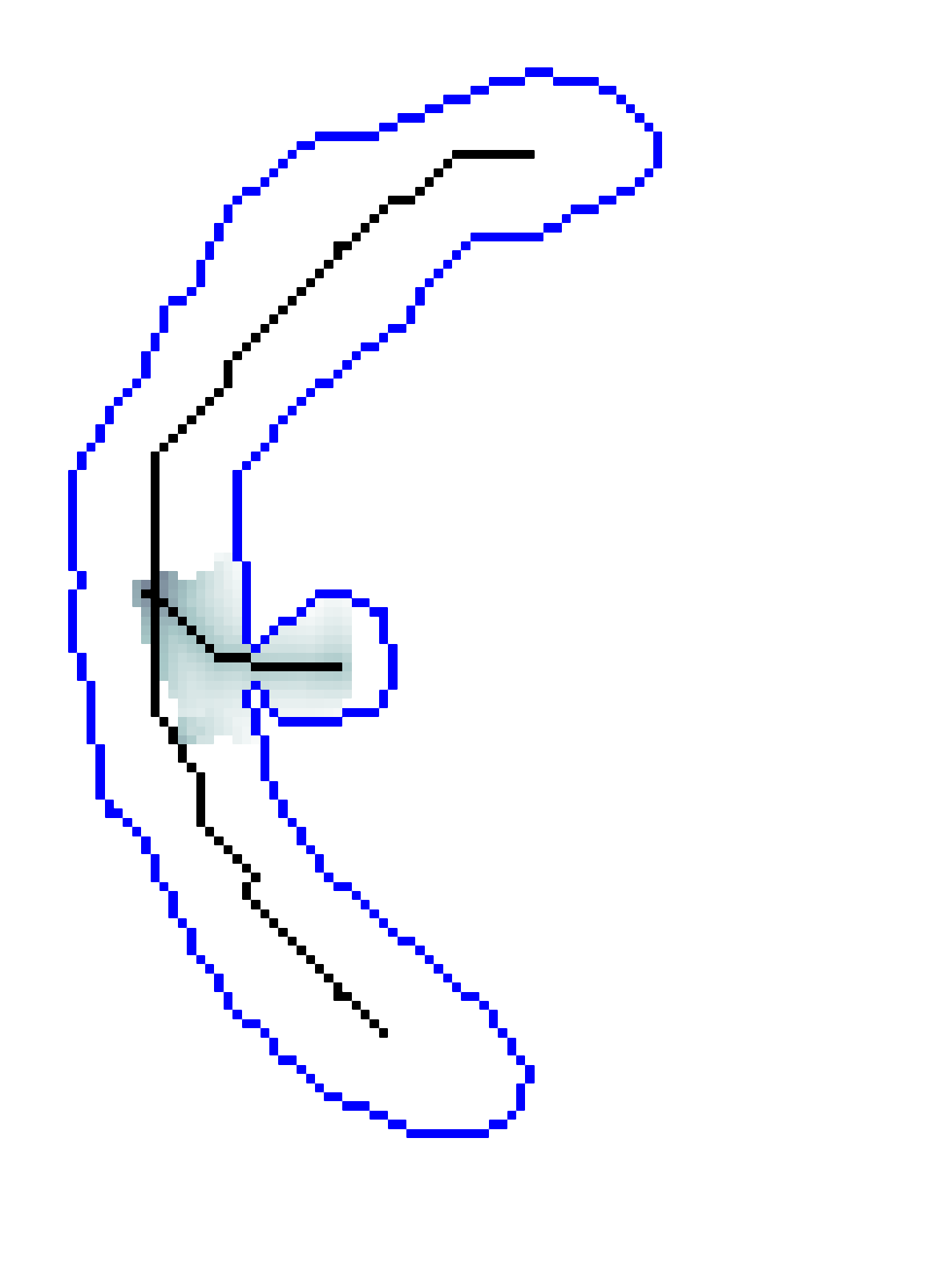
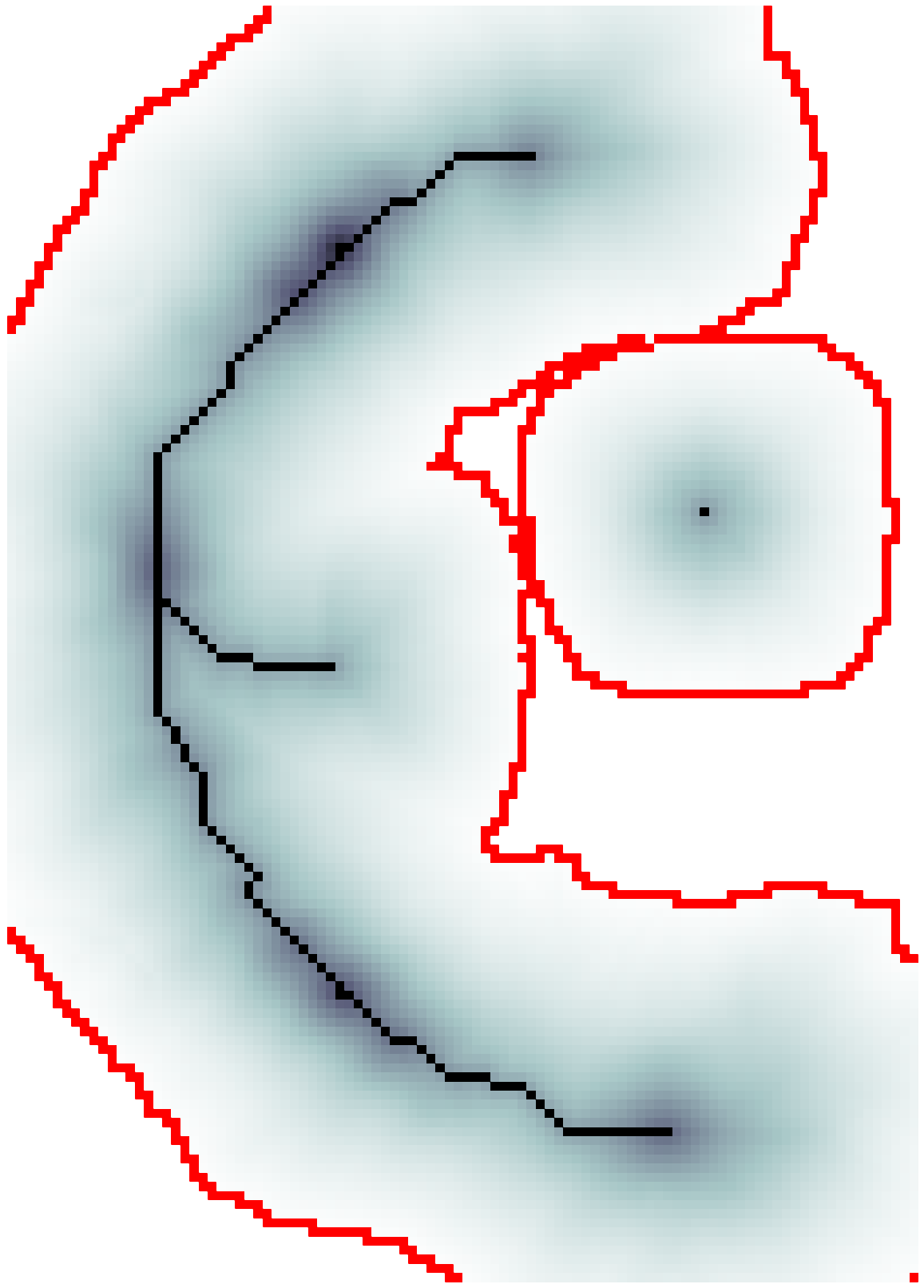
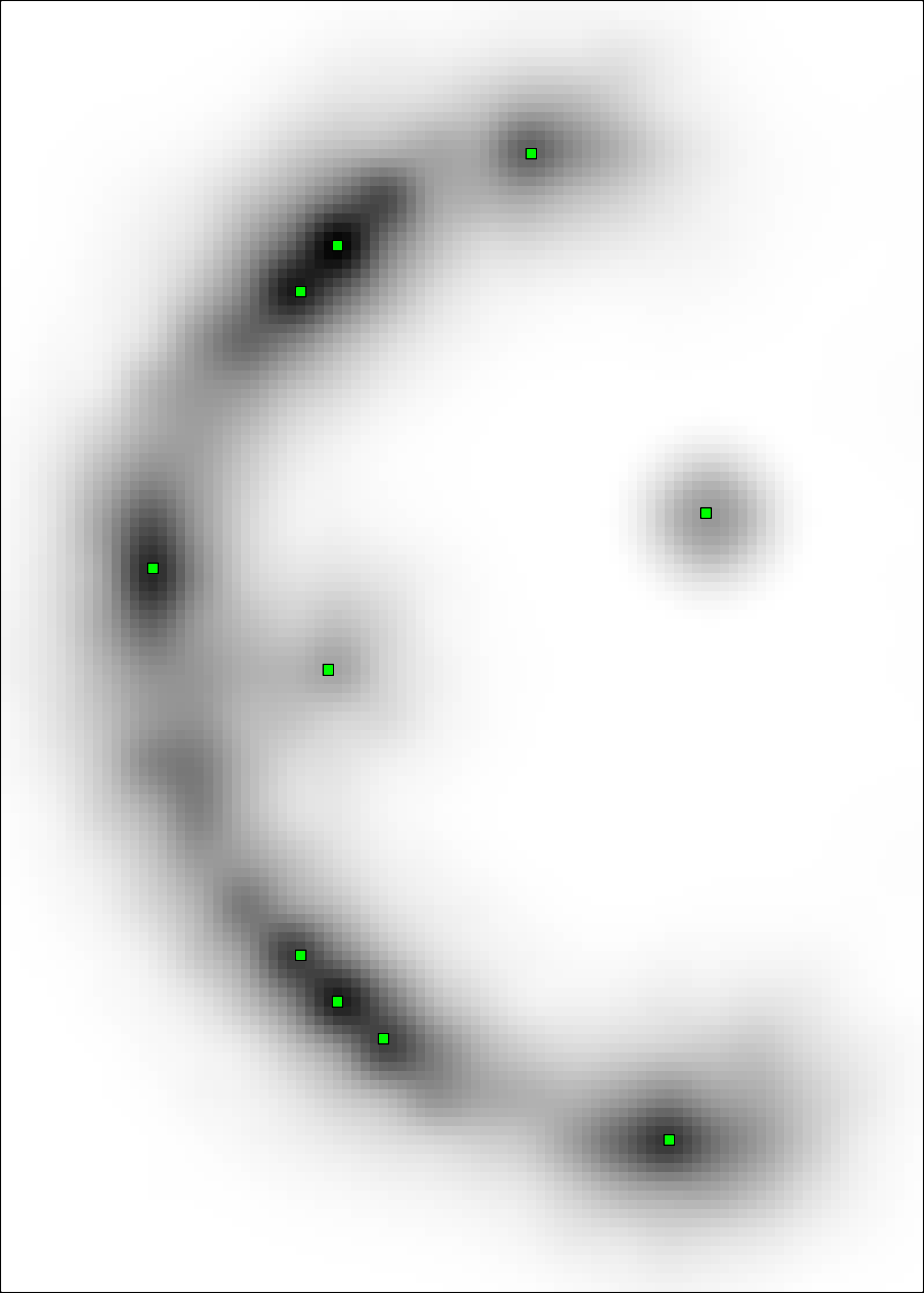
	$\mathcal{V}$
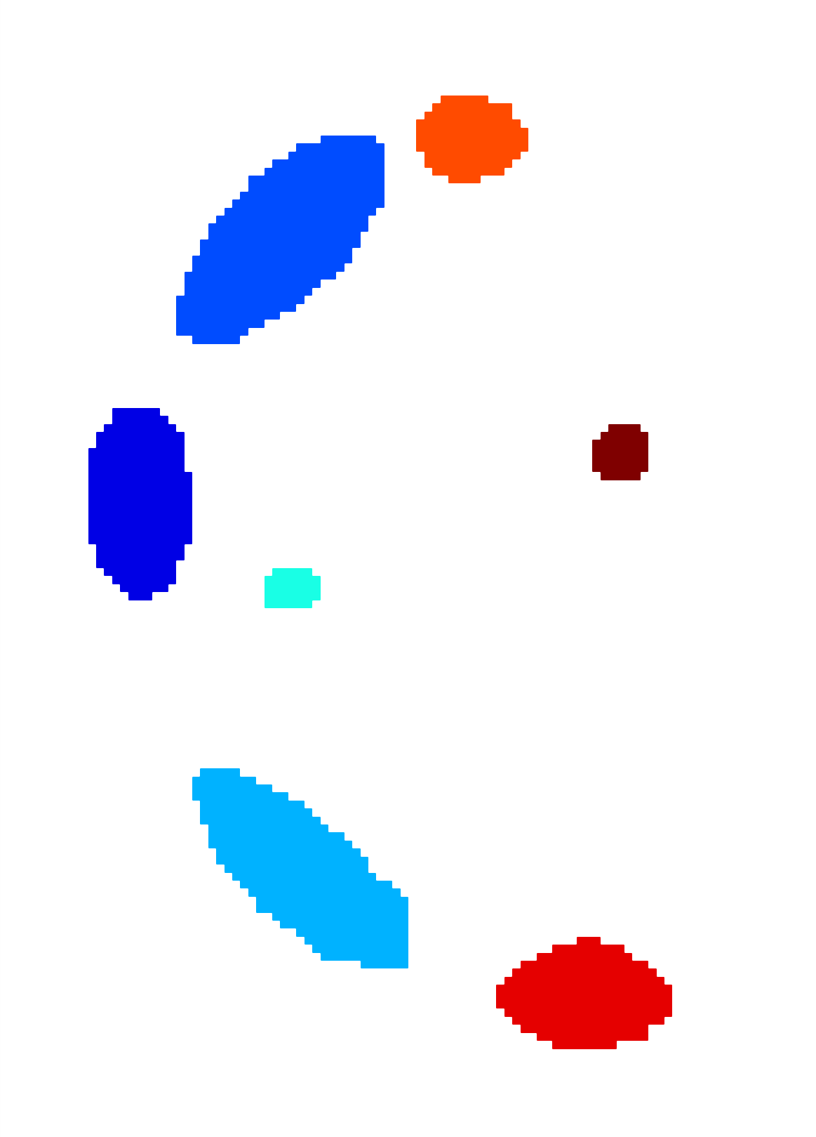
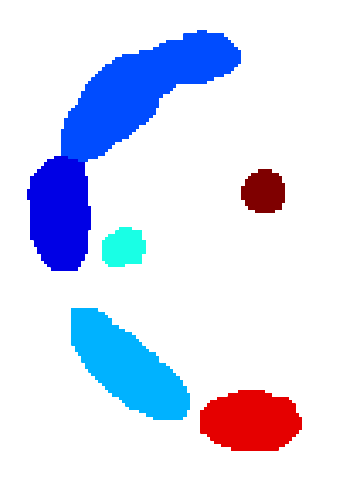
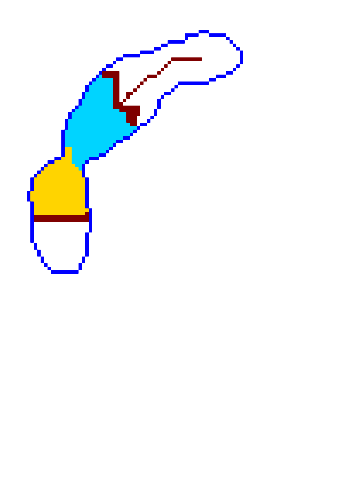
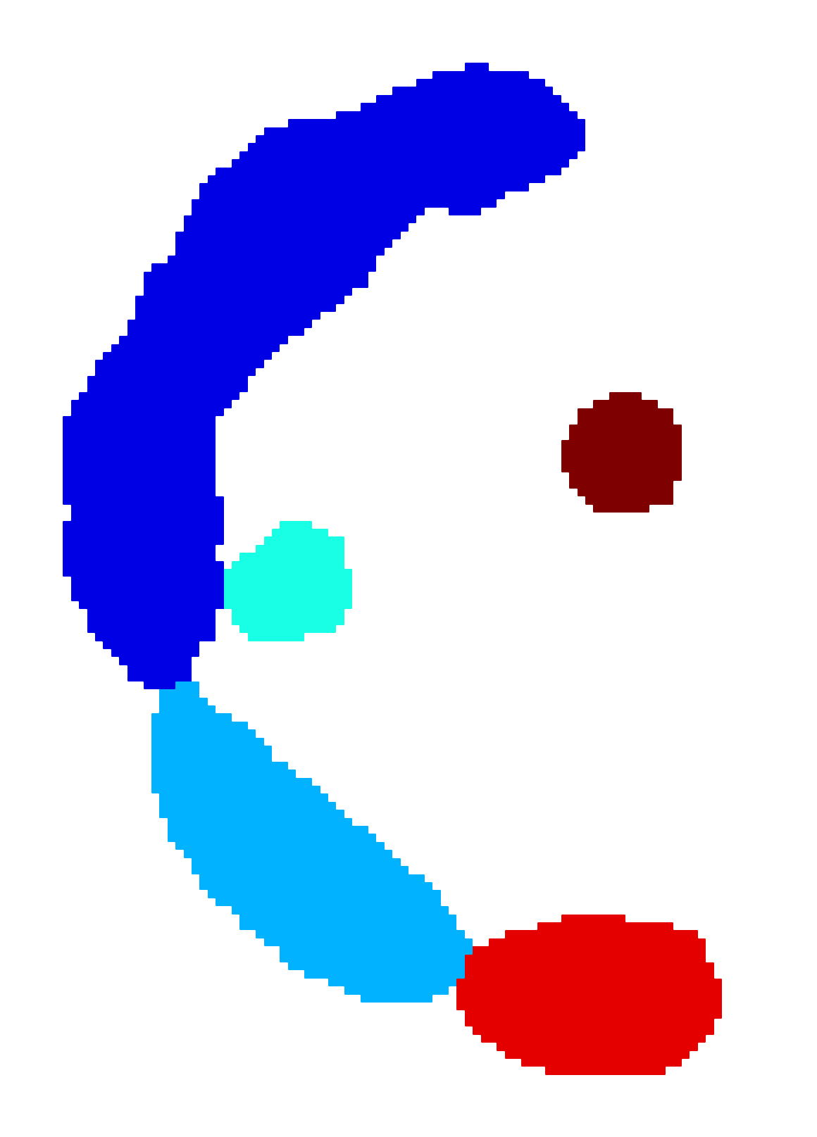
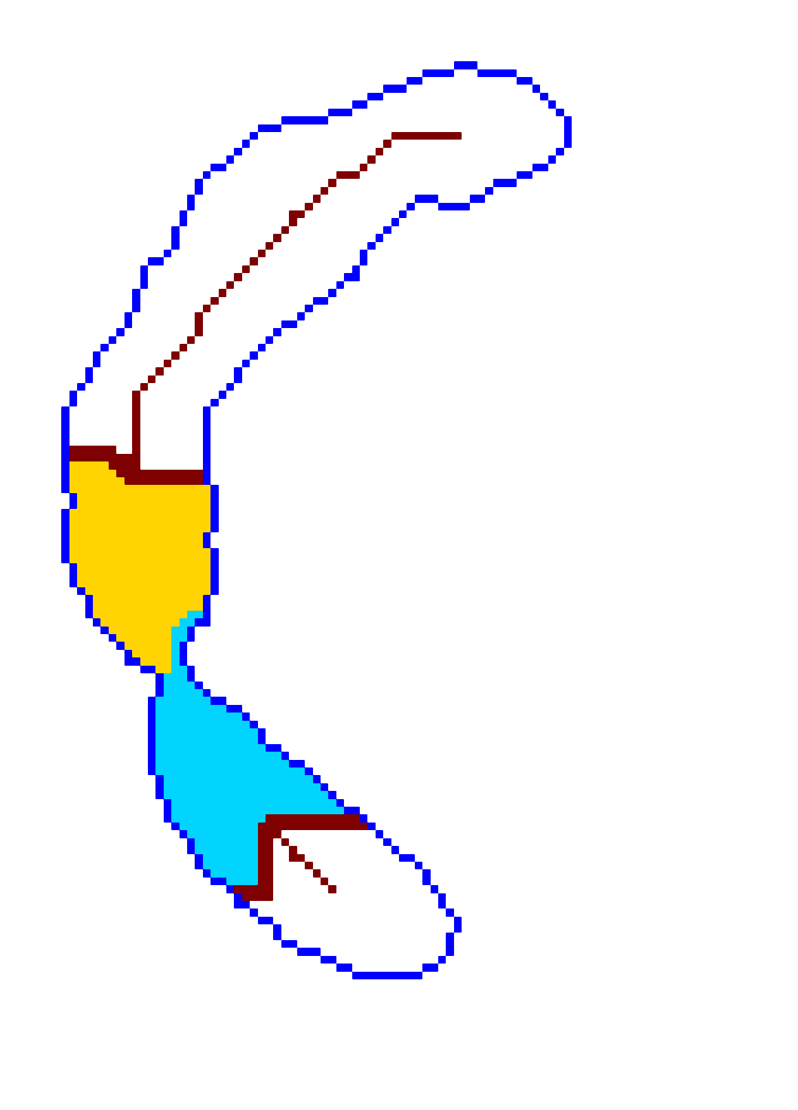
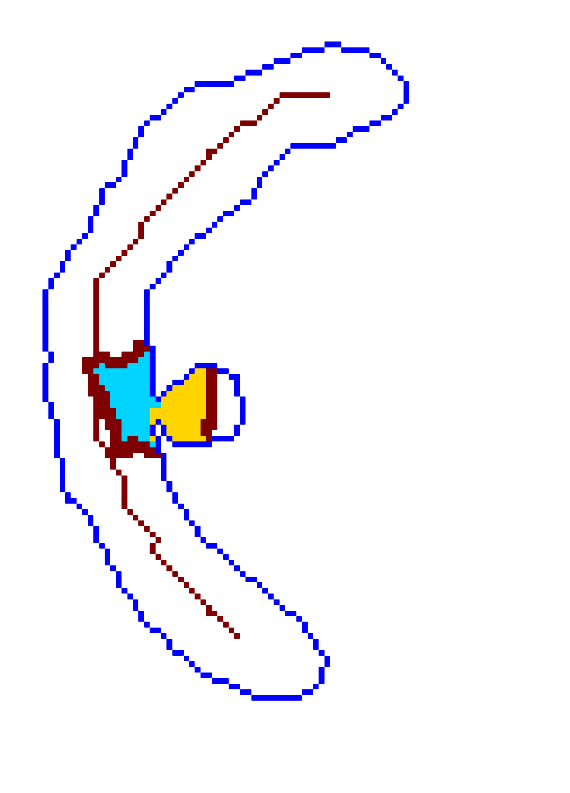
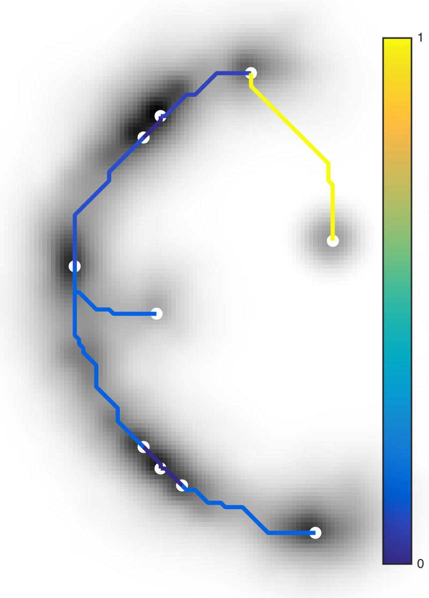
$\mathcal{P}\cup S$				$(A\cup B)^{\text{{{u}}}}$		$(A\cup B)^{\text{{{u}}}}$		$(A\cup B)^{\text{{{u}}}}$	Geodesic U

Figure 2: Sequential acyclic connectivity paradigm on a synthetic 2D image.

3 Experiments and Results

3.0.1 Dataset.

A 3D hand-crafted tortuous and convoluted phantom (HCP) is designed to account for complex vessel patterns, i.e. branching, kissing vessels, scale and shape variations induced by pathologies. Also a set of 20 synthetic vascular trees (SVT) ($64\times 64\times 64$ voxels) were generated using VascuSynth [10] considering two levels of additional noise (N₁: $\mathcal{N}(0,5)$ + Shadows: 1 + Salt$\&$Pepper: $1\permil$;   N₂: $\mathcal{N}(0,10)$ + Shadows: 1 + Salt$\&$Pepper: $2\permil$). Together with the synthetic data, a cerebral Phase Contrast MRI (PC) ($0.86\times 0.86\times 1.0$ mm), a cerebral Time of Flight MRI (TOF) ($0.36\times 0.36\times 0.5$ mm) and a carotid CTA ($0.46\times 0.46\times 0.45$ mm) were used. Vascular network ground-truths (GT) are given in the form of connected raster centerlines for all the synthetic images and for both TOF and CTA.

3.0.2 Experiments.

The scalar vesselness responses of both HCP and PC images are determined using the state-of-the-art Frangi filter (FFR) [8], and Optimally Oriented Flux (OOF) [12]. Also, the connected vesselness map (CVM) and the associated tensor field (TF) are synthesized for the same dataset using VTrails. The connectedness of the considered scalar maps is qualitatively assessed and the TF is inspected as proof of concept in section 3.1.
VTrails is used to extract the connected geodesic paths for all the synthetic SVT and for TOF and CTA images. In section 3.2, each set of connected geodesic paths is verified to be an acyclic graph, then it is compared against the respective GT. The robustness to image degradation, the accuracy, precision and recall are evaluated voxel-wise for the identified branches with a tolerance factor $\varrho$ as in [1].

	Image	FFR	OOF	CVM	TF
HCP
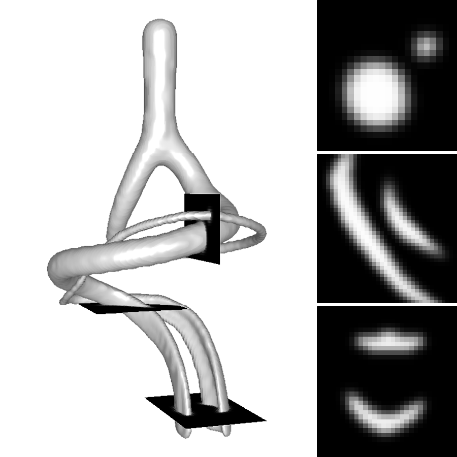
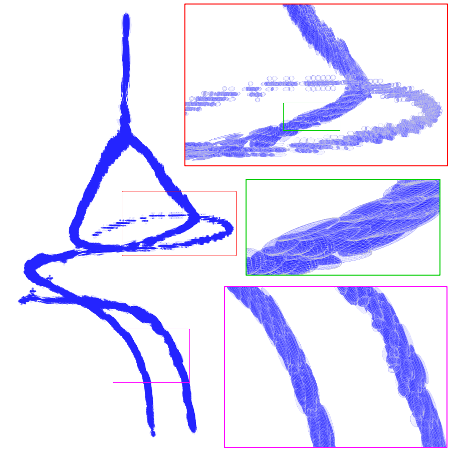
PC

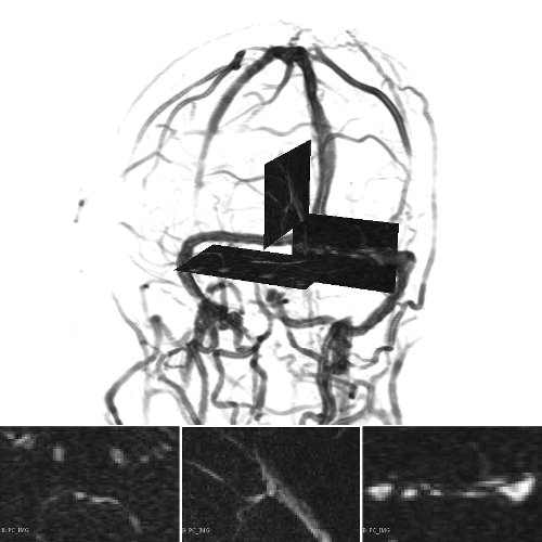
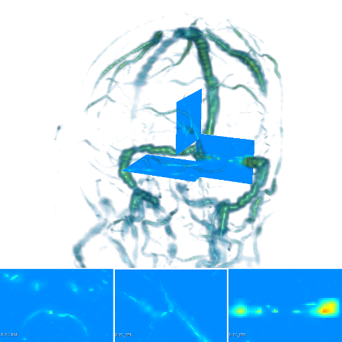
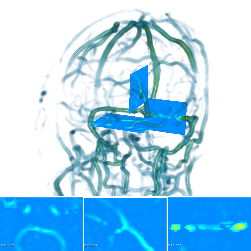
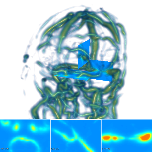
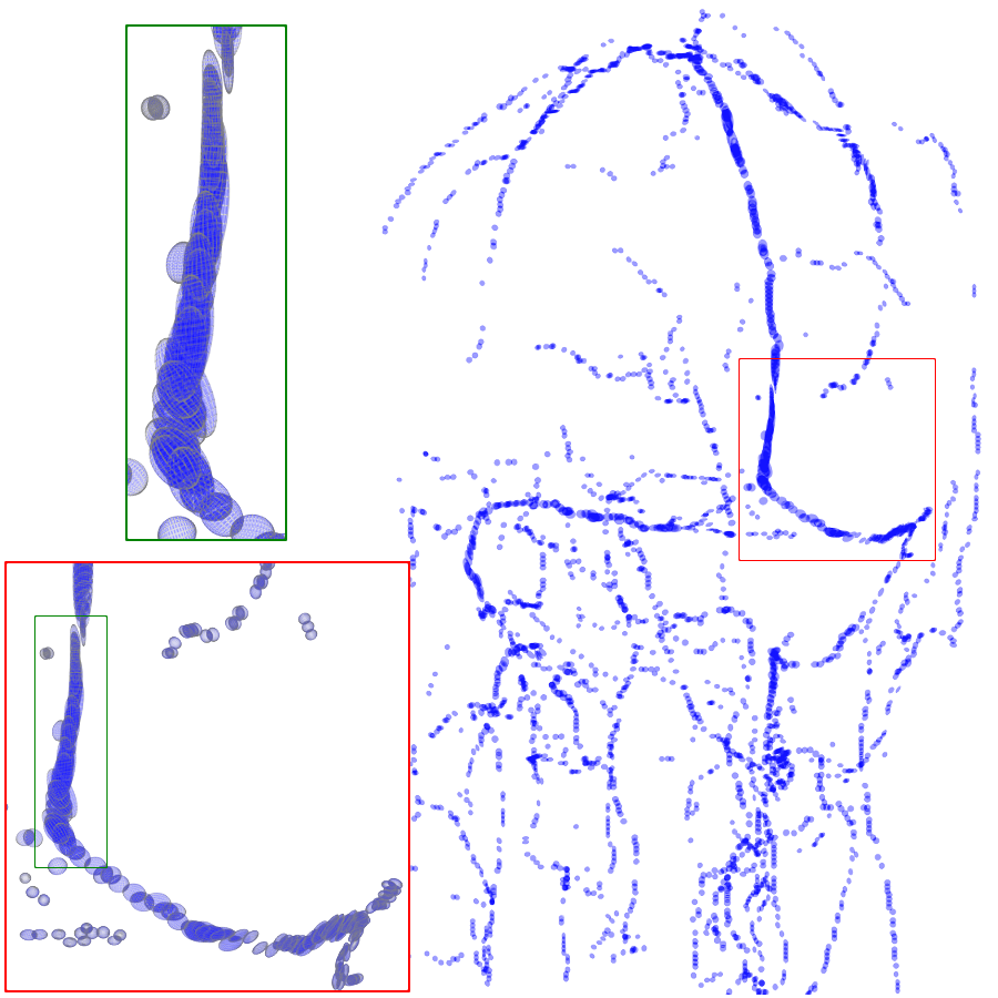
Figure 3: Vesselness response maps for Frangi, OOF, and proposed scalar CVM with associated tensor field on a digital phantom example and on data of a phase contrast cerebral venogram.

3.1 Connectedness of the Vesselness Map

Fig. 3 shows the connectedness of vessels recovered from state-of-the-art vascular enhancers and curvilinear ridge detectors FFR and OOF together with the proposed CVM for the synthetic HCP and the real PC images. On the synthetic phantom, FFR shows a fragmented and rough vesselness response in correspondence of irregularly shaped sections of the structure. Also, the response at the bifurcation is not smoothly connected with the branches (triangular loop). Conversely, OOF recovers the phantom connectedness at the branch-point, and the vesselness response is consistent along the tortuous curvilinear section, however ghosting artifacts are observed as the shape of the phantom becomes irregular (C-like) or differs from a cylindrical tube. Also, close convoluted structures, which change scale rapidly in the HCP, produce inconsistent responses of OOF (fig. 3). CVM shows here a strongly connected vesselness response in correspondence of both regular and irregular tubular sections, with local maxima at structures’ mid-line. The connectedness of the structures is emphasized regardless the complexity of the shape, and it resolves spatially the tortuous curvilinear ‘kissing vessels’ without additional ghosting artifacts, despite the smooth profile.
Similar results are observed on the PC dataset: FFR has a poor connected response in the noisy and low-resolution image. Vessels are overall enhanced, however thin and fragmented structures remain disconnected. Overall, the vesselness response is not uniform within the noisy structures, where maximal values are often off-centred. A more consistent response is obtained from OOF, where the connectedness of vessels is improved. Maximal response is observed at the mid-line of vessels, however, noise rejection is poor. CVM strongly enhances here the vessel connectivity. The fragmented vessels of PC have a continuous and smooth response in CVM with higher values and a more defined profile. Large vessels shows solid connected regions with local maxima at mid-line as in OOF. Conversely from OOF, CVM shows improved noise rejection in the background.
The respective tensor fields (TF) synthesized on both HCP and PC show consistent features. The TF’s characteristics are in line with the connectedness of CVM: enhanced and connected vessels are associated with high anisotropy, whereas background areas show a predominant isotropic component.

3.2 Connected Geodesic Paths as Vascular Tree

Representative examples of degraded synthetic images from SVT and the respective GT are shown in fig. 4 together with the connected graphs extracted by VTrails. Analogously, the same set of images are reported for the real images TOF and CTA in fig. 4. Qualitatively, the extracted set of connected geodesic paths shows remarkable matching with the provided GT in all cases. First, we verify the acyclic nature of the graph. We found no cycles, degenerate graphs and unconnected nodes, meaning that the extracted connected geodesic paths represent a connected geodesic tree. Precision and recall are then evaluated for the identified branches. Also, error distances are determined as the connected tree’s binary distance map evaluated at GT. Average errors ($\overline{\varepsilon}$) precision and recall are reported (mean$\pm$SD) in table 1. Note that no pruning of any spurious branches is performed in the analysis.

Synthetic Vascular Trees (SVT) [10]				Clinical Angiographies
	Image	GT	VTrails		Image	GT	VTrails
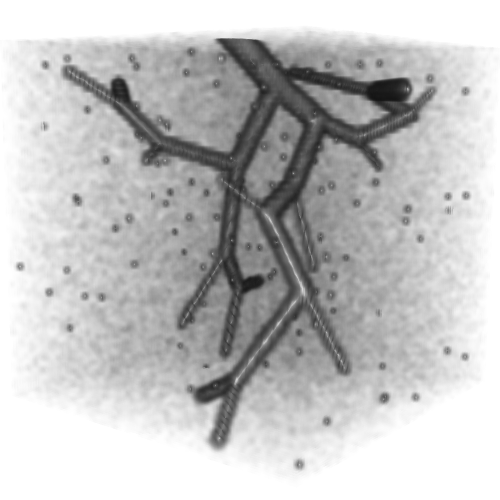
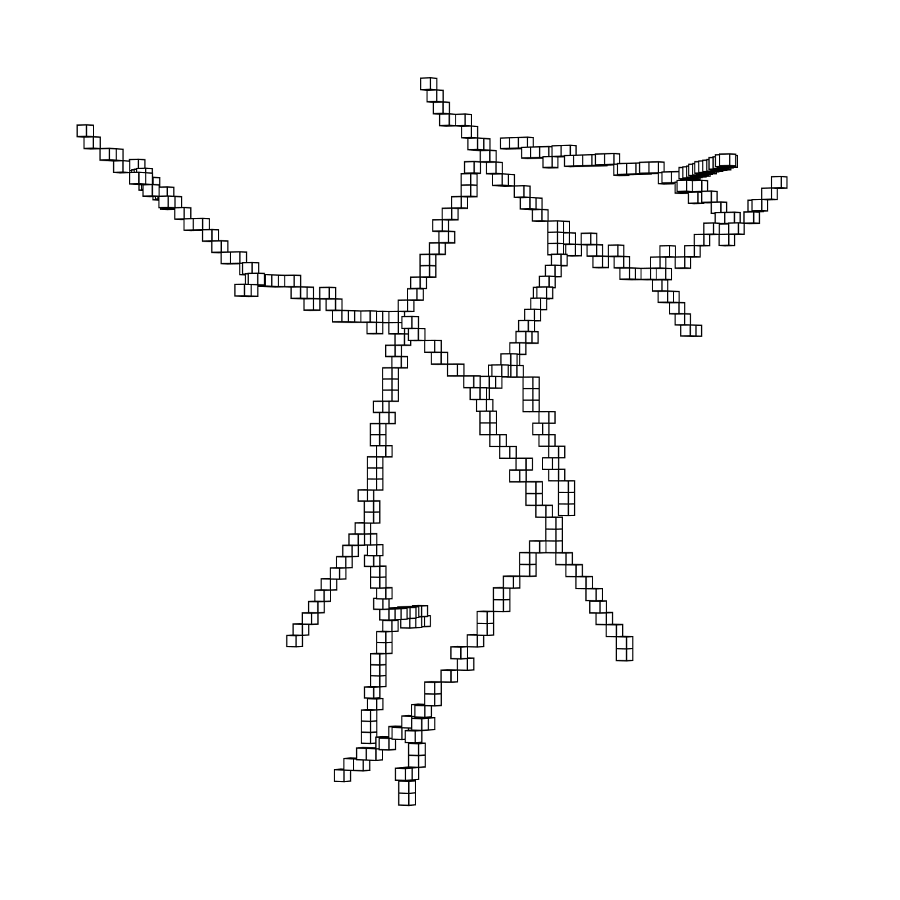
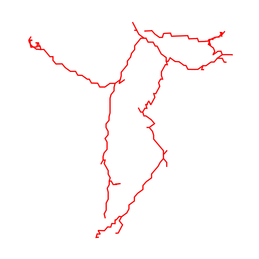
N1				CTA
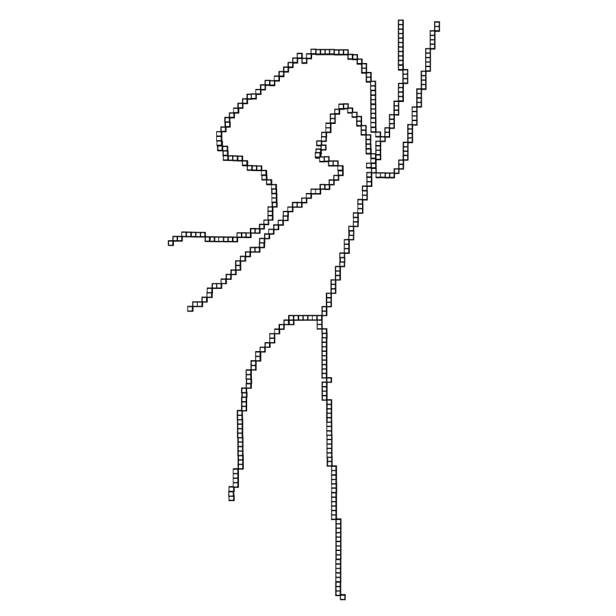
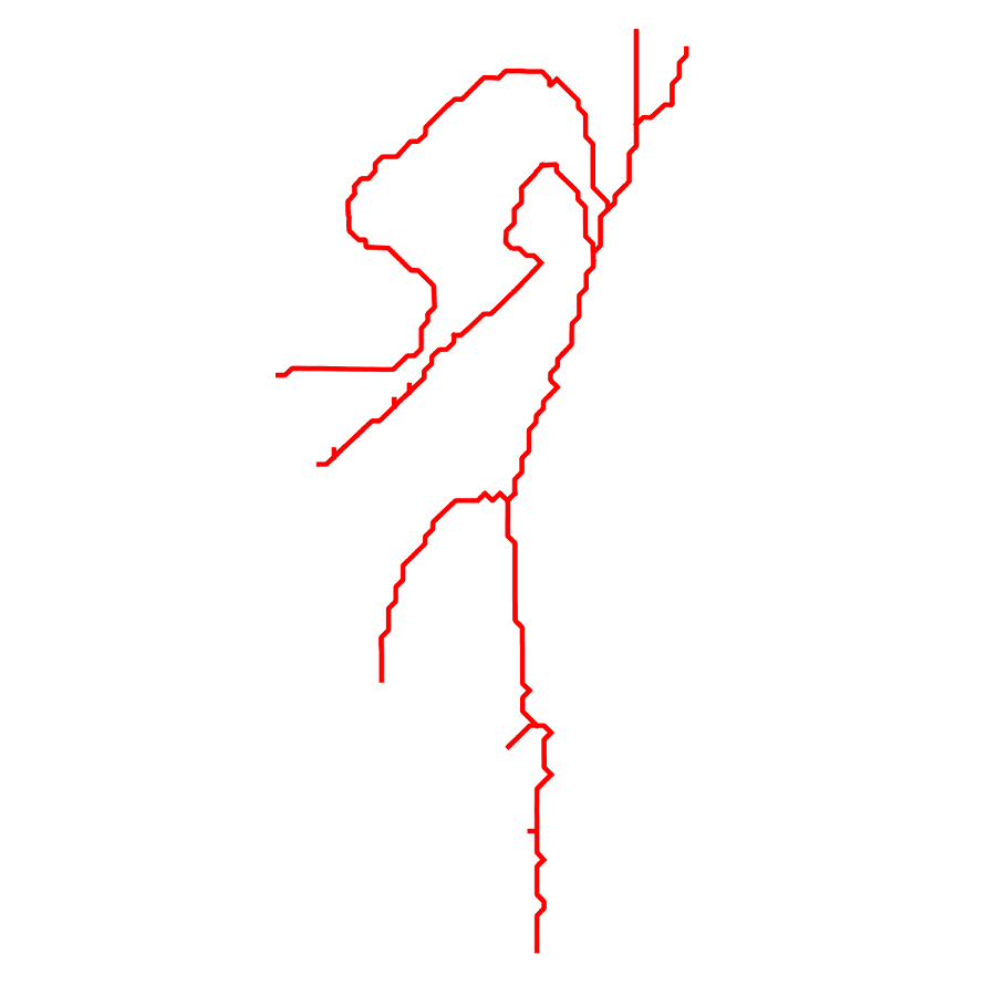
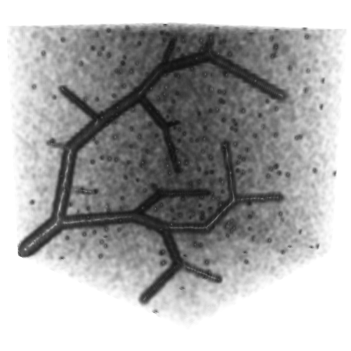
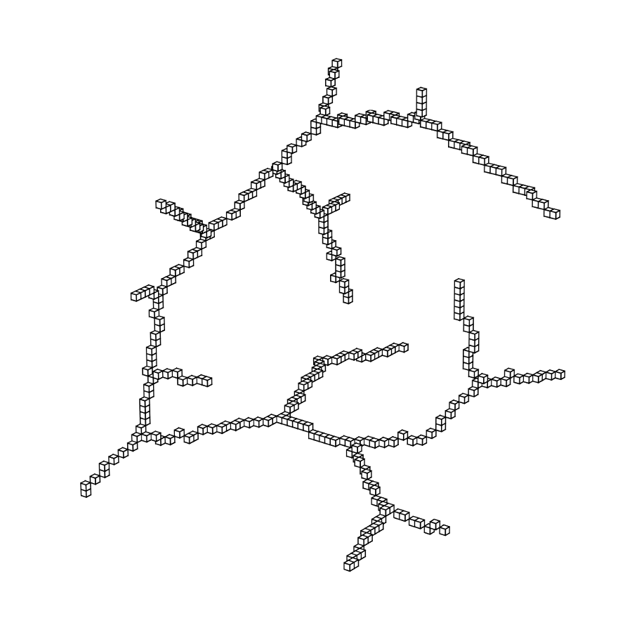
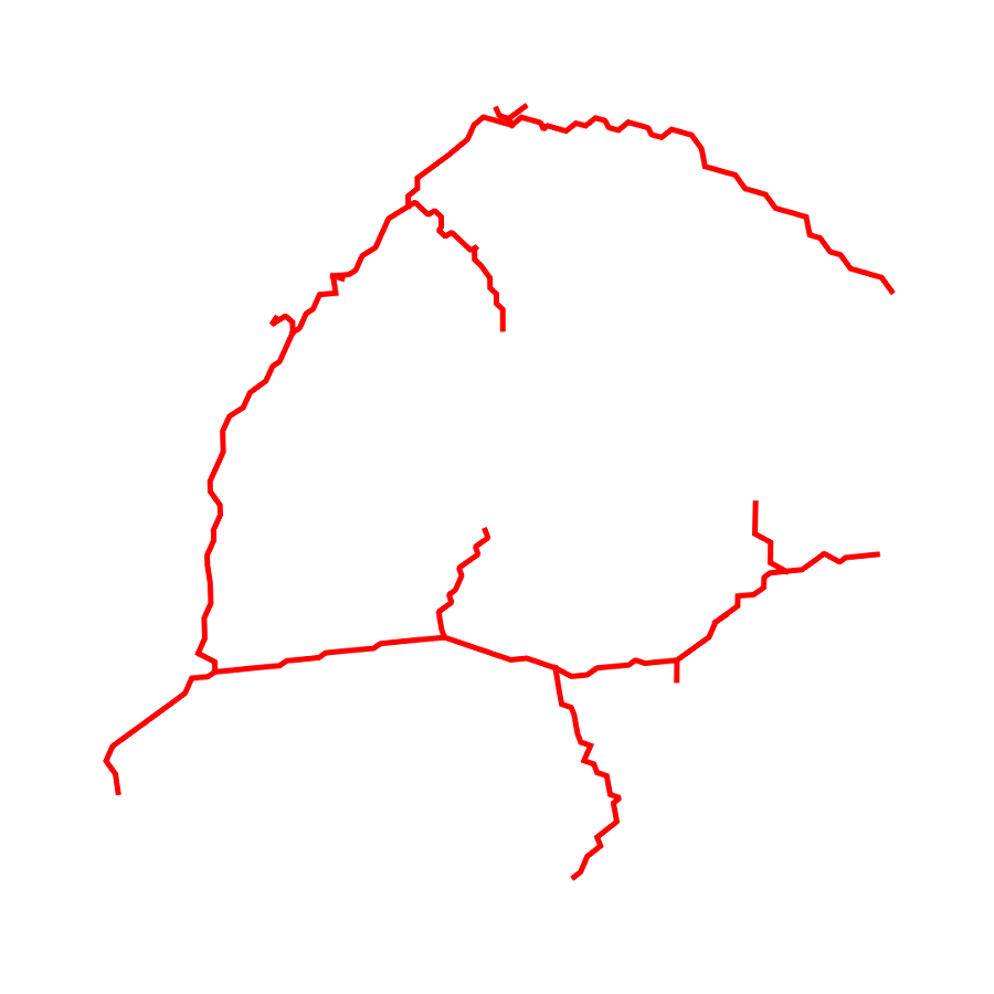
N2				TOF

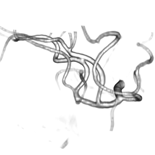
Figure 4: Comparison of the vascular connected trees against the relative ground-truth for a representative set of synthetic data, and for a carotid CTA and for a middle cerebral artery TOF MRI. Note that main branches are correctly identified and connected.

4 Discussion and Conclusions

We presented VTrails, a novel connectivity-oriented method for vascular image analysis. The proposed method has the advantage of introducing the SLoGS filterbank, which simultaneously synthesizes a connected vesselness map and the associated tensor field in the same mathematically coherent framework. Interestingly, recent works [17, 9] are exploring Riemannian manifolds of tensors for high-order vascular metrics, however the coherent definition of a tensor field is not trivial for an arbitrary scalar image, as its topology cannot be generally approximated simply by an ellipsoid model [14]. The steerability property of SLoGS stands out as key feature for i. reducing the dimensionality of the kernels parameters in 3D, ii. determining the filterbank’s rotation-invariance and iii. optimizing the 3D filtering complexity in the OLA. Also, the combined rotation- and curvature-invariance of the filtering process results in branch-points that coincide with the locally integrated center of mass of the multiple SLoGS filter responses. This explains the strong response in the CVM at the branch-point in fig. 3. Regarding the acyclic connectivity paradigm employed in VTrails, we experimentally verified that the resulting set of connected geodesic paths $\Pi$ forms a tree. The assumption of a vascular tree provides a natural and anatomically valid constraint for 3D vascular images, with few rare exceptions, such as the complete circle of Willis [5]. It is important to note that the proposed algorithm can include extra anatomical constraints to correct for locations where the vascular topology is not acyclic or where noise it too high. Note that despite the optimal formulation of the anisotropic front propagation, a limitation of the greedy acyclic connectivity paradigm is the possibility of miss-connecting branches, potentially disrupting the topology of the vascular network. Overall, promising results have been reported from this early validation, with a fully-automatic extraction configuration. Missing branches occur in correspondence of small vessels, where the effect of degradation is predominant: tiny terminal vessels completely occluded by the corrupting shadows will not automatically produce seeds, hence cannot be recovered under such configuration. Globally, $\overline{\varepsilon}$ values are comparable to the evaluation tolerance $\varrho$, suggesting that the connected geodesic paths extracted by VTrails lie in the close neighbourhood of the vessels’ centerlines. Moreover, the reported values are comparable regardless the level of degradation. Future developments will address the optimization of the CVM integration strategy in section 2.1 to account for an equalized response over the vascular spatial frequency-bands. Also, the topological analysis of vascular networks on a population of subjects will be investigated in future works to better embed priors in the acyclic connectivity paradigm.

		Synthetic Vascular Trees [10]			Clinical Angiographies
		N1	N2		TOF	CTA
$\overline{\varepsilon}$	[voxels]	$2.15\pm 0.65$	$2.09\pm 0.37$	[mm]	$1.07\pm 2.65$	$1.1\pm 1.63$
$\varrho$		2			1.42	1.57
Precision		$88.21\pm 2.58\%$	$87.93\pm 2.56\%$		$77.12\%$	$89.67\%$
Recall		$68.31\pm 7.44\%$	$69.18\pm 3.69\%$		$89.49\%$	$83.97\%$

Table 1: Connectivity tree error distances, precision and recall (mean$\pm$SD): (left) synthetic vascular tree at degradation levels N₁ and N₂; (right) TOF and CTA. Note the invariance of all metrics regardless the degradation level.

References

- [1] R. Annunziata, A. Kheirkhah, P. Hamrah, and E. Trucco. Scale and curvature invariant ridge detector for tortuous and fragmented structures. In MICCAI 2015.
- [2] L. Antiga, M. Piccinelli, L. Botti, B. Ene-Iordache, A. Remuzzi, and D. A. Steinman. An image-based modeling framework for patient-specific computational hemodynamics. Med. Biol. Eng. Comput., 2008.
- [3] V. Arsigny, P. Fillard, X. Pennec, and N. Ayache. Log-euclidean metrics for fast and simple calculus on diffusion tensors. Magn. Reson. Med., 2006.
- [4] F. Benmansour and L. D. Cohen. Tubular structure segmentation based on minimal path method and anisotropic enhancement. Int. J. Comput. Vision, 2011.
- [5] R. A. Bergman, A. K. Afifi, and R. Miyauchi. Illustrated encyclopedia of human anatomic variation: Circle of Willis. www.anatomyatlases.org/AnatomicVariants/.
- [6] E. Bullitt, S. Aylward, A. Liu, J. Stone, S. K. Mukherji, C. Coffey, G. Gerig, and S. M. Pizer. 3D graph description of the intracerebral vasculature from segmented mra and tests of accuracy by comparison with x-ray angiograms. In IPMI 1999.
- [7] M. J. Cardoso, M. Modat, T. Vercauteren, and S. Ourselin. Scale factor point spread function matching: beyond aliasing in image resampling. In MICCAI 2015.
- [8] A. F. Frangi, W. J. Niessen, K. L. Vincken, and M. A. Viergever. Multiscale vessel enhancement filtering. In MICCAI 1998.
- [9] M. A. Gülsün, G. Funka-Lea, P. Sharma, S. Rapaka, and Y. Zheng. Coronary centerline extraction via optimal flow paths and cnn path pruning. In MICCAI 2016.
- [10] G. Hamarneh and P. Jassi. Vascusynth: simulating vascular trees for generating volumetric image data with ground-truth segmentation and tree analysis. Comput. Med. Imag. Graph., 2010.
- [11] R. Kwitt, D. Pace, M. Niethammer, and S. Aylward. Studying cerebral vasculature using structure proximity and graph kernels. In MICCAI 2013.
- [12] M. W. Law and A. C. Chung. Three dimensional curvilinear structure detection using optimally oriented flux. In ECCV 2008.
- [13] D. Lesage, E. D. Angelini, I. Bloch, and G. Funka-Lea. A review of 3D vessel lumen segmentation techniques: Models, features and extraction schemes. Med. Image Anal., 2009.
- [14] Q. Lin. Enhancement, extraction, and visualization of 3D volume data. 2003.
- [15] A. V. Oppenheim and R. W. Schafer. Discrete-time signal processing. Pearson Higher Education, 2010.
- [16] M. Schaap, R. Manniesing, I. Smal, T. Van Walsum, A. Van Der Lugt, and W. Niessen. Bayesian tracking of tubular structures and its application to carotid arteries in cta. In MICCAI 2007.
- [17] C. Wang, M. Oda, Y. Hayashi, Y. Yoshino, T. Yamamoto, A. F. Frangi, and K. Mori. Tensor-based graph-cut in riemannian metric space and its application to renal artery segmentation. In MICCAI 2016.
- [18] M. A. Zuluaga, R. Rodionov, M. Nowell, S. Achhala, G. Zombori, A. F. Mendelson, M. J. Cardoso, A. Miserocchi, A. W. McEvoy, J. S. Duncan, and S. Ourselin. Stability, structure and scale: improvements in multi-modal vessel extraction for seeg trajectory planning. Int. J. Comput. Assist. Radiol. Surg., 2015.