On the approximation of $SBD$ functions
and some applications

Abstract.

Three density theorems for three suitable subspaces of $SBD$ functions, in the strong $BD$ topology, are proven. The spaces are $SBD$, $SBD^{p}_{\infty}$, where the absolutely continuous part of the symmetric gradient is in $L^{p}$, with $p>1$, and $SBD^{p}$, whose functions are in $SBD^{p}_{\infty}$ and the jump set has finite $\mathcal{H}^{n-1}$-measure. This generalises on the one hand the density result [12] by Chambolle and, on the other hand, extends in some sense the three approximation theorems in [29] by De Philippis, Fusco, Pratelli for $SBV$, $SBV^{p}_{\infty}$, $SBV^{p}$ spaces, obtaining also more regularity for the absolutely continuous part of the approximating functions. As application, the sharp version of two $\Gamma$-convergence results for energies defined on $SBD^{2}$ is derived.

1. Introduction

The study of free discontinuity functionals has required the introduction of suitable ambient spaces, such as the Functions of Bounded Variations $BV$ and of Bounded Deformation $BD$, with corresponding subspaces and generalisations.

A $L^{1}$ function $u$ is in $BV$ [respectively in $BD$] if its distributional gradient $\mathrm{D}u$ [resp. its distributional symmetric gradient ${\mathrm{E}}u=(\mathrm{D}u+\mathrm{D}^{T}u)/2$] is a bounded Radon measure. In particular, a $BD$ function is defined from a set $\Omega\subset{{\mathbb{R}}}^{n}$ into ${{\mathbb{R}}}^{n}$. The measure $\mathrm{D}u$ [${\mathrm{E}}u$] is decomposed into three parts: one absolutely continuous with respect to $\mathcal{L}^{n}$, with density $\nabla u$ [$e(u)$], one supported on the rectifiable $(n{-}1)$-dimensional jump set $J_{u}$, where $u$ has two different approximate limits $u^{+}$, $u^{-}$ on the two sides of $J_{u}$ with respect to an approximate normal $\nu_{u}\in{\mathbb{S}^{n-1}}$, and a Cantor part, vanishing on Borel sets of finite $\mathcal{H}^{n-1}$ measure. $SBV$ [$SBD$] is the space of $BV$ [$BD$] functions with null Cantor part. Here we consider also, for $p>1$, the subspaces

$$SBD^{p}(\Omega):=\{u\in SBD(\Omega)\colon e(u)\in L^{p}(\Omega;{\mathbb{M}^{n\times n}_{sym}})\,,\ \mathcal{H}^{n-1}(J_{u})<\infty\}$$

and

$$SBD^{p}_{\infty}(\Omega):=\{u\in SBD(\Omega)\colon e(u)\in L^{p}(\Omega;{\mathbb{M}^{n\times n}_{sym}})\}\,$$

with analogous definitions for $SBV^{p}(\Omega)$ and $SBV^{p}_{\infty}$ (see Section 2 for more details).

The spaces $SBD^{p}$ are very important in Fracture Mechanics: if $u$ represents the displacement of a body from its equilibrium configuration, $J_{u}$ is nothing but the crack set and $e(u)$ is the linearised elastic strain, which is in $L^{2}$ (so $p=2$) if the material is linearly elastic in the bulk region. For many years after the introduction of $SBD$ in [3], $SBD^{2}$ has been employed to study brittle fracture, namely the Griffith energy

$$\int\limits_{\Omega}\mathbb{C}e(u)\colon e(u)\,\mathrm{d}x+\mathcal{H}^{n-1}(J_{u})\,,$$ (G)

$\mathbb{C}$ being the (fourth-order positive definite) Cauchy stress tensor, with possibly lower order terms due to forces, and boundary conditions. Unfortunately, the corresponding compactness and lower semicontinuity theorem [9] requires equi-integrability of displacements, which is not guaranteed for a sequence with bounded (G) energy. Indeed, the right ambient space for (G) is $GSBD^{2}$, introduced by Dal Maso in [27], with the corresponding compactness and lower semicontinuity theorem proven very recently in [19] (see also [36] in dimension 2).

The first density result for $SBD^{2}$, due to Chambolle ([12, 13]) consists then in the approximation, with respect to the energy (G), of $u\in SBD^{2}\cap L^{2}$ by functions smooth outside their jump set, in turn closed and included in a finite union of $C^{1}$ hypersurfaces (this has been extended to $GSBD^{p}$ in [38, 35, 23, 18]).

If we are given an energy controlling the amplitude of the jump $[u]:=u^{+}-u^{-}$ in $L^{1}(J_{u};{{\mathbb{R}}}^{n})$, in contrast to Griffith energy that controls only the measure of $J_{u}$, then $SBD^{p}$ (for a $p$-growing bulk energy) is the proper ambient space. This is the case, for $p=2$, of the energy

$$\int\limits_{\Omega}\mathbb{C}e(u)\colon e(u)\,\mathrm{d}x+\mathcal{H}^{n-1}(J_{u})+\int\limits_{J_{u}}\big{|}[u]\odot\nu_{u}\big{|}\,\mathrm{d}\mathcal{H}^{n-1}\,,$$ (C)

($\odot$ being the symmetric tensor product) considered by Focardi and Iurlano in [32], and recently in [11]. A fracture energy depending on $[u]$, as (C), is often called cohesive, in contrast to the brittle energy (G).

In order to deal with energies such as (C), the following approximation theorem for $SBD^{p}$, that involves also the jump part of ${\mathrm{E}}u$, is proven. This is the main result of the paper.

Theorem 1.1.

Let $\Omega$ be an open bounded Lipschitz subset of ${{\mathbb{R}}}^{n}$, and $u\in SBD^{p}(\Omega)$, with $p>1$. Then there exist $u_{k}\in SBV^{p}(\Omega;{{\mathbb{R}}}^{n})\cap L^{\infty}(\Omega;{{\mathbb{R}}}^{n})$ such that each $J_{u_{k}}$ is closed and included in a finite union of closed connected pieces of $C^{1}$ hypersurfaces, $u_{k}\in C^{\infty}(\overline{\Omega}\setminus J_{u_{k}};{{\mathbb{R}}}^{n})\cap W^{m,\infty}(\Omega\setminus J_{u_{k}};{{\mathbb{R}}}^{n})$ for every $m\in{\mathbb{N}}$, and:

$$\lim_{k\to\infty}\Big{(}\|u_{k}-u\|_{BD(\Omega)}+\|e(u_{k})-e(u)\|_{L^{p}(\Omega;{\mathbb{M}^{n\times n}_{sym}})}+\mathcal{H}^{n-1}(J_{u_{k}}\triangle J_{u})\Big{)}=0\,.$$ (1.1a)

Moreover, (if $$p\in\big{[}1,\frac{n}{n-1}\big{]} E_{k}\subset\Omega$$ this is trivial) there are Borel sets such that

$$\lim_{k\to\infty}\mathcal{L}^{n}(E_{k})=\lim_{k\to\infty}\int\limits_{\Omega\setminus E_{k}}|u_{k}-u|^{p}\,\mathrm{d}x=0\,.$$ (1.1b)

The theorem above is sharp, in the sense that it provides the strongest possible approximation of all the relevant quantities in the definition of $SBD^{p}$. In particular, it improves the density result [12, 13] since Theorem 1.1 allows even the approximation of the jump part of ${\mathrm{E}}u$, that is not possible with the previous results. Moreover, differently from [12, 13] that assume $u\in L^{2}$, it does not require any additional integrability assumption on $u$, and it is valid for any $p>1$ (in [23] it is observed that the construction in [12, 13] does not work for $p\neq 2$). These characteristics are in common with the sharp density result in $GSBD^{p}$ [18], which employs a similar construction, here improved to deal with $[u]$, see below.

We remark that [38] and [18] approximate also any truncation of $[u]$, but this is not enough to deal with energies such as (C) without assuming a priori a uniform $L^{\infty}$ bound. Notice also that the assumptions on $\Omega$ could be weakened, also in the following Theorems (see Remark 4.2).

It is interesting to compare Theorem 1.1 with available density results in $SBV^{p}$, where of course there are more tools, such as the maximum principle or the coarea formula, due to the control on all $\nabla u$. On the one hand, Theorem 1.1 may be combined with weaker $SBV^{p}$ approximations, but through functions with more regular jump set; on the other hand, our result provides stronger properties (some weaker) with respect to the available approximations in $BV$ norm for $SBV^{p}$, giving the possibility to improve them.

First we consider the theorem by Cortesani and Toader, that approximates functions in $SBV^{p}\cap L^{\infty}$ with respect to an energy

$$\int\limits_{\Omega}|\nabla u|^{p}\,\mathrm{d}x+\mathcal{H}^{n-1}(J_{u})+\int\limits_{J_{u}}\phi(x,u^{+},u^{-},\nu_{u})\,\mathrm{d}\mathcal{H}^{n-1}\,,$$ (C’)

for very general $\phi$ (cf. Theorem 6.1, see also the earlier [30] for a weaker result, and [1] for an approximation for $BV\cap L^{\infty}$ functions). The approximating functions are of class $C^{\infty}\cap W^{m,\infty}$, for every $m\in{\mathbb{N}}$, outside the jump set, in turn closed and contained in a finite union of $(n{-}1)$-simplexes. Of course, this additional regularity on the jump set is in general in contrast to convergence in $BV$-norm.

The first approximation result in $BV$-norm, for functions in $SBV^{p}\cap L^{\infty}$, is due to Braides and Chiadò-Piat [10]: the approximating functions $u_{k}$ are $C^{1}$ outside some closed rectifiable sets $R_{k}$, such that $J_{u_{k}}\subset R_{k}$, with no information on the shape of $J_{u_{k}}$.

In the recent paper [29], De Philippis, Fusco, and Pratelli approximate $SBV^{p}$ functions by means of $u_{k}$ in $C^{\infty}(\Omega\setminus J_{u_{k}})$, with $J_{u_{k}}$ a compact $C^{1}$ manifold, up to a $\mathcal{H}^{n-1}$-negligible set, and

$$\lim_{k\to\infty}\Big{(}\|u_{k}-u\|_{BV(\Omega;{\mathbb{R}}^{m})}+\|\nabla(u_{k})-\nabla(u)\|_{L^{p}(\Omega;\mathbb{M}^{m{\times}n})}+\mathcal{H}^{n-1}(J_{u_{k}}\triangle J_{u})\Big{)}=0\,.$$

The main improvement due to Theorem 1.1, besides the fact that it holds in $SBD^{p}$, is that our $u_{k}$ are also in $W^{m,\infty}(\Omega\setminus J_{u_{k}})$, for every $m\in{\mathbb{N}}$, that may be important in the applications; for instance the “by hand constructions” for the $\Gamma$-$\limsup$ in Theorems 6.3 and 6.5 (cf. [32, 11]), or in [17], have to be done for functions that are Lipschitz up to the jump set (even if for these particular applications one could use also the density in Theorem 6.1). A possible weakness of our result is the fact that $J_{u_{k}}$ is not a $C^{1}$ manifold, even if, for the applications that we imagine at the moment (also for those presented in [29]), one needs just $J_{u_{k}}$ closed, or one may employ [25] (see also Remark 5.4).

In [29] also two approximations in $BV$-norm, respectively for $SBV$ and $SBV^{p}_{\infty}$, are shown. In the spirit of this work, we prove the following approximations for $SBD$ and $SBD^{p}_{\infty}$. As in Theorem 1.1, we assume that $\Omega$ is open bounded Lipschitz. The crucial property is indeed that the trace of $u$ is integrable on $\partial\Omega$, so one could weaken the regularity assumption on $\Omega$.

Theorem 1.2.

Let $u\in SBD(\Omega)$. Then there exist $u_{k}\in SBD(\Omega)\cap L^{\infty}(\Omega;{{\mathbb{R}}}^{n})$ such that $J_{u_{k}}$ is, up to a $\mathcal{H}^{n-1}$-negligible set, a finite union of pairwise disjoint $C^{1}$ compact hypersurfaces contained (strictly) in $\Omega$, $u_{k}\in C^{\infty}(\overline{\Omega}\setminus J_{u_{k}};{{\mathbb{R}}}^{n})\cap W^{m,\infty}(\Omega\setminus J_{u_{k}};{{\mathbb{R}}}^{n})$, and

$$\lim_{k\to\infty}\big{(}\|u_{k}-u\|_{BD(\Omega)}+\mathcal{H}^{n-1}(J_{u_{k}}\triangle J_{u})\big{)}=0\,.$$ (1.2)

Theorem 1.3.

Let $u\in SBD^{p}_{\infty}(\Omega)$, with $p>1$. Then there exist $u_{k}\in SBV^{p}(\Omega;{{\mathbb{R}}}^{n})\cap L^{\infty}(\Omega;{{\mathbb{R}}}^{n})$ such that each $J_{u_{k}}$ is closed and included in a finite union of closed connected pieces of $C^{1}$ hypersurfaces, $u_{k}\in C^{\infty}(\overline{\Omega}\setminus J_{u_{k}};{{\mathbb{R}}}^{n})\cap W^{m,\infty}(\Omega\setminus J_{u_{k}};{{\mathbb{R}}}^{n})$ for every $m\in{\mathbb{N}}$, and:

$$\lim_{k\to\infty}\Big{(}\|u_{k}-u\|_{BD(\Omega)}+\|e(u_{k})-e(u)\|_{L^{p}(\Omega;{\mathbb{M}^{n\times n}_{sym}})}\Big{)}=0\,.$$ (1.3)

We observe that in Theorem 1.2 we have also the full regularity of $J_{u_{k}}$, so this in fact generalises [29, Theorem A] allowing us to consider $SBD(\Omega)$ and $u_{k}$ of class $W^{m,\infty}$ outside $J_{u_{k}}$. (Indeed we employ [29, Lemma 4.3] to pass from $J_{u_{k}}$ included in, to $J_{u_{k}}$ essentially equal to the finite union of the desired $C^{1}$ hypersurfaces.)

As for the approximation in $SBD^{p}_{\infty}$, we are not able to guarantee that $\mathcal{H}^{n-1}(J_{u_{k}}\setminus J_{u})$ vanishes. This issue is also present in the corresponding [29, Theorem B], so Theorem 1.3 is not sharp (cf. Remark 5.3).

In all the previous theorems, notice the strong convergence of $u_{k}$ to $u$ in $BD$ implies that (see (2.1) and $|a||b|/\sqrt{2}\leq|a\odot b|\leq|a||b|$ for every $a$, $b$ in ${{\mathbb{R}}}^{n}$)

$$\int\limits_{J_{u}\cup J_{u_{k}}}\big{|}[u]-[u_{k}]\big{|}\,\mathrm{d}\mathcal{H}^{n-1}\to 0\,.$$

We conclude this introduction by briefly describing the proof strategy and possible applications of our results.

In all the three theorems, we assume $u$ extended with 0 outside $\Omega$, and we start from a set $\widehat{\Gamma}\in C^{1}$ with $\mathcal{H}^{n-1}(\widehat{\Gamma}\setminus J_{u})$ and $\int_{J_{u}\setminus\widehat{\Gamma}}\big{|}[u]\big{|}\,\mathrm{d}\mathcal{H}^{n-1}$ small. In the spirit of [12], we cover $\widehat{\Gamma}$ by hypercubes $Q_{j}$ split almost in two halves by this hypersurface, and we apply a rough approximation procedure in the complement of the union of the hypercubes, and in both sides of any cube with respect to $\widehat{\Gamma}$.

We need different rough approximations for the $SBD^{p}$ and $SBD^{p}_{\infty}$ case, provided by Theorem 3.1 and Proposition 5.2, respectively, while for Theorem 1.2 a suitable convolution is enough. The idea behind any rough approximation is to partition a given domain by hypercubes of sidelength $Ck^{-1}$ and to detect the bad hypercubes, i.e. those where the jump energy (or, similarly, the measure of the jump set for $SBD^{p}$) is not controlled well: in these hypercubes (indeed also in the adjacent boundary good hypercubes) one sets $u_{k}$ as the infinitesimal rigid motion which is the “mean” of $u$, while in the remaining good hypercubes one employs either a Korn-Poincaré-type inequality provided by [14] (cf. Proposition 2.3), or Lemma 5.1, or a convolution with a radial kernel supported on a ball of radius $k^{-1}$, in correspondence to each of the three density results. This construction differs from that of the rough approximation in [18, Theorem 3.1], where $u_{k}=0$ on the bad hypercubes, because we were there interested mainly in the measure of $J_{u_{k}}$, and not to control $[u_{k}]$.

A fundamental point is to separate the sets on which we employ the rough approximation: first, this requires the function to be defined in a small neighbourhood of any subset, to have the room for convolution; the second issue is to glue all the pieces obtained from the rough approximations in each subset. These problems could be solved by the technique in [12], at the expense of assuming a priori $u\in L^{p}$, since partitions of unity are needed, or by the trick in [18], that employs also an extension argument derived from Nitsche [42] (see Lemma 2.1). Now there is a further delicate issue: if we glue as in [18] we are not able to control $[u_{k}]$ on the intersection between $\partial Q_{j}$ and the zone where we extend by Lemma 2.1, even if this has small $\mathcal{H}^{n-1}$ measure. For this reason we have to perform a very careful approximation procedure, keeping the reflected zone of height $Ck^{-1}$, so comparable to the size of small hypercubes and of the convolution kernels.

A key difference with respect to [29] is that the rough approximants are smooth in a neighbourhood of any piece, so gluing them we keep the regularity up to the jump. This is not the case if one employs variable convolution kernels whose size decreases close to $\widehat{\Gamma}$, as in [29].

As application, we present an improvement to the sharp version of two $\Gamma$-convergence approximations by phase-field energies à la Ambrosio-Tortorelli (cf. [5]) for the energy (C), in [32] and [11] (we mention also some approximations for cohesive energies [20, 28, 8]). In [32] and [11], the $\Gamma$-limsup inequality was proven just in $SBD^{2}\cap L^{\infty}$, because this was done by hand for the regular functions provided by the Cortesani-Toader approximation, and then extended by [38]. Now it is enough to apply Theorem 1.1 to pass directly to $SBD^{2}$, without any further integrability assumption.

We give no direct application to Theorems 1.2 and 1.3, but we recall that [29, Theorem 6.1] proves a representation formula for the total variation of $\mathrm{D}u$ for $BV$ and $SBV$ functions, derived from the analogous of Theorem 1.2 in [29].

In general, the result presented could be abstract tools useful to extend a variety of $\Gamma$-convergence approximations for e.g. suitable cohesive-type energies, that might be for instance in terms of finite elasticity or non-local energies, see respectively [33] and [40, 41] for the case of Griffith energy.

The plan of the paper is the following. In Section 2 we fix the notation and recall some technical lemmas, in Section 3 we present the rough approximation for Theorem 1.1, which is completely proven in Section 4. Section 5 is devoted to prove the other two density results, and the applications are contained in Section 6.

2. Notation and preliminaries

We denote by $\mathcal{L}^{n}$ and $\mathcal{H}^{k}$ the $n$-dimensional Lebesgue measure and the $k$-dimensional Hausdorff measure. For any locally compact subset $B$ of ${{\mathbb{R}}}^{n}$, the space of bounded ${\mathbb{R}}^{m}$-valued Radon measures on $B$ is indicated as $\mathcal{M}_{b}(B;{\mathbb{R}}^{m})$. For $m=1$ we write $\mathcal{M}_{b}(B)$ for $\mathcal{M}_{b}(B;{\mathbb{R}})$ and $\mathcal{M}^{+}_{b}(B)$ for the subspace of positive measures of $\mathcal{M}_{b}(B)$. For every $\mu\in\mathcal{M}_{b}(B;{\mathbb{R}}^{m})$, $|\mu|(B)$ stands for its total variation. We use the notation: $\chi_{E}$ for the indicator function of any $E\subset{\mathbb{R}}^{n}$, which is 1 on $E$ and 0 otherwise; $B_{\varrho}(x)$ for the open ball with center $x$ and radius $\varrho$; $x\cdot y$, $|x|$ for the scalar product and the norm in ${{\mathbb{R}}}^{n}$; $p^{*}$ for $np/(n-p)$, $n$ being the space dimension; $\mathrm{diam}(E)$ for the diameter of $E$.

$BV$ and $BD$ functions.

For $U\subset{{\mathbb{R}}}^{n}$ open, a function $v\in L^{1}(U)$ is a function of bounded variation on $U$, denoted by $v\in BV(U)$, if $\mathrm{D}_{i}v\in\mathcal{M}_{b}(U)$ for $i=1,\dots,n$, where $\mathrm{D}v=(\mathrm{D}_{1}v,\dots,\mathrm{D}_{n}v)$ is its distributional gradient. A vector-valued function $v\colon U\to{\mathbb{R}}^{m}$ is $BV(U;{\mathbb{R}}^{m})$ if $v_{j}\in BV(U)$ for every $j=1,\dots,m$.

The space of functions of bounded deformation on $U$ is

$$BD(U):=\{v\in L^{1}(U;{{\mathbb{R}}}^{n})\colon{\mathrm{E}}v\in\mathcal{M}_{b}(U;{\mathbb{M}^{n\times n}_{sym}})\}\,,$$

where ${\mathrm{E}}v$ is the distributional symmetric gradient of $v$. It is well known (see [3, 43]) that $BD(U)$ is a Banach space with the norm

$$\|v\|_{BD(U)}=\|v\|_{L^{1}(U;{{\mathbb{R}}}^{n})}+|{\mathrm{E}}v|(U)\,,$$

and that, for $v\in BD(U)$, the jump set $J_{v}$, defined as the set of points $x\in U$ where $v$ has two different one sided Lebesgue limits $v^{+}(x)$ and $v^{-}(x)$ with respect to a suitable direction $\nu_{v}(x)\in{\mathbb{S}^{n-1}}$, is countably $(\mathcal{H}^{n-1},n-1)$ rectifiable (see, e.g. [31, 3.2.14]), and that

$$\mathrm{E}v=\mathrm{E}^{a}v+\mathrm{E}^{c}v+\mathrm{E}^{j}v\,,$$

where $\mathrm{E}^{a}v$ is absolutely continuous with respect to $\mathcal{L}^{n}$, $\mathrm{E}^{c}v$ is singular with respect to $\mathcal{L}^{n}$ and such that $|\mathrm{E}^{c}v|(B)=0$ if $\mathcal{H}^{n-1}(B)<\infty$, while

$${\mathrm{E}}^{j}v=[v]\odot\nu_{v}\,\mathcal{H}^{n-1}\mathbin{\vrule height=6.2pt,depth=0.0pt,width=0.50375pt\vrule height=0.50375pt,depth=0.0pt,width=5.03749pt}J_{v}\,.$$ (2.1)

In the above expression of ${\mathrm{E}}^{j}v$, $[v]$ denotes the jump of $v$ at any $x\in J_{v}$ and is defined by $[v](x):=(v^{+}-v^{-})(x)$, the symbols $\odot$ and $\mathbin{\vrule height=6.2pt,depth=0.0pt,width=0.50375pt\vrule height=0.50375pt,depth=0.0pt,width=5.03749pt}$ stands for the symmetric tensor product and the restriction of a measure to a set, respectively. Since $|a\odot b|\geq|a||b|/\sqrt{2}$ for every $a$, $b$ in ${{\mathbb{R}}}^{n}$, it holds $[v]\in L^{1}(J_{v};{{\mathbb{R}}}^{n})$. The density of $\mathrm{E}^{a}v$ with respect to $\mathcal{L}^{n}$ is denoted by $e(v)$, and we have that (see [3, Theorem 4.3]) for $\mathcal{L}^{n}$-a.e. $x\in U$

$$\lim_{\varrho\to 0^{+}}\frac{1}{\varrho^{n}}\int\limits_{B_{\varrho}(x)}\frac{\big{(}v(y)-v(x)-e(v)(x)(y-x)\big{)}\cdot(y-x)}{|y-x|^{2}}\mathrm{d}y=0\,.$$

The space $SBD(U)$ is the subspace of all functions $v\in BD(U)$ such that $\mathrm{E}^{c}v=0$, while for $p\in(1,\infty)$

$$SBD^{p}(U):=\{v\in SBD(U)\colon e(v)\in L^{p}(U;{\mathbb{M}^{n\times n}_{sym}}),\,\mathcal{H}^{n-1}(J_{v})<\infty\}\,.$$

Analogous properties hold for $BV$, as the countable rectifiability of the jump set and the decomposition of $\mathrm{D}v$. Similarly, $SBV(U;{\mathbb{R}}^{m})$ is the space of $BV(U;{\mathbb{R}}^{m})$ with null Cantor part and

$$SBV^{p}(U;{\mathbb{R}}^{m}):=\{v\in SBV(U;{\mathbb{R}}^{m})\colon\nabla v\in L^{p}(U;\mathbb{M}^{m{\times}n}),\,\mathcal{H}^{n-1}(J_{v})<\infty\}\,,$$

$\nabla v$ denoting the density of $\mathrm{D}^{a}v$, the absolutely continuous part of $\mathrm{D}v$, with respect to $\mathcal{L}^{n}$. Consider also the space (for this notation see e.g. [29])

$$SBV^{p}_{\infty}(U;{\mathbb{R}}^{m}):=\{v\in SBV(U;{\mathbb{R}}^{m})\colon\nabla v\in L^{p}(U;\mathbb{M}^{m{\times}n})\}\,,$$

and its analogue

$$SBD^{p}_{\infty}(U):=\{v\in SBD(U)\colon e(v)\in L^{p}(U;{\mathbb{M}^{n\times n}_{sym}})\}\,.$$

For more details on the spaces $BV$, $SBV$ and $BD$, $SBD$ we refer to [4] and to [3, 9, 7, 43], respectively. Below we recall some other properties that will be useful in the following.

We start with an extension lemma derived from [42, Lemma 1]. The result is employed in dimension 2 in [21, Lemma 3.4], and formulated in the more general setting of the space $GSBD^{p}$ in [36, Lemma 5.2] and in [18, Lemma 2.8], to which we refer for more details of the proof.

Lemma 2.1.

Let $R\subset{{\mathbb{R}}}^{n}$ be an open hyperrectangle (in dimension $n$) , $R^{\prime}$ be the reflection of $R$ with respect to one face $F$ of $R$, and $\widehat{R}$ be the union of $R$, $R^{\prime}$, and $F$. Let $p\in(1,\infty)$ and $v\in SBD^{p}(R)$. Then $v$ may be extended by a function $\widehat{v}\in SBD^{p}(\widehat{R})$ such that

$$\mathcal{H}^{n-1}(J_{\widehat{v}} \cap F)=0\,,$$ (2.2a)

$$\|\widehat{v}\|_{L^{1}(\widehat{R})} \leq c\|v\|_{L^{1}(R)}$$ (2.2b)

$$\mathcal{H}^{n-1}(J_{\widehat{v}}) \leq c\,\mathcal{H}^{n-1}(J_{v})\,,$$ (2.2c)

$$\int\limits_{J_{\widehat{v}}}|[\widehat{v}]|\,\mathrm{d}\mathcal{H}^{n-1} \leq c\int\limits_{J_{v}}|[v]|\,\mathrm{d}\mathcal{H}^{n-1}\,,$$ (2.2d)

$$\int\limits_{\widehat{R}}|e(\widehat{v})|^{p}\,\mathrm{d}x \leq c\,\int\limits_{R}|e(v)|^{p}\,\mathrm{d}x\,,$$ (2.2e)

for a suitable $c>0$ independent of $R$ and $v$. Moreover, the result is still true if $v\in SBD(R)$, with $p=1$ in (2.2e), or if $v\in SBD^{p}_{\infty}(R)$ (when $\mathcal{H}^{n-1}(J_{v})=\infty$, (2.2c) says nothing) with extensions $\widehat{v}$ in $SBD(\widehat{R})$ or in $SBD^{p}_{\infty}(\widehat{R})$, respectively.

Proof.

We may follow [18, Lemma 2.8], stated for $v\in GSBD^{p}(R)$. We assume that $F\subset\{(x^{\prime},x_{n})\in{\mathbb{R}}^{n-1}\times{\mathbb{R}}\colon x_{n}=0\}$ and $R\subset\{(x^{\prime},x_{n})\in{\mathbb{R}}^{n-1}\times{\mathbb{R}}\colon x_{n}<0\}$, fix any $\mu$, $\nu$ such that $0<\mu<\nu<1$, and let $q:=\frac{1+\nu}{\nu-\mu}$. Then

$$\widehat{v}:=\begin{dcases}v\quad&\text{in }R\,,\\ v^{\prime}\quad&\text{in }R^{\prime}\,,\end{dcases}$$

for $v^{\prime}$ defined on $R^{\prime}$ by

$$v^{\prime}:=q\,v_{A_{\mu}}+(1-q)v_{A_{\nu}}\,,$$

with $A_{\mu}=\mathrm{diag}\,(1,\dots,1,-\mu)$, $A_{\nu}=\mathrm{diag}\,(1,\dots,1,-\nu)$, and for any $u\in SBD^{p}(\Omega)$, $A\in M^{n{\times}n}$

$$u_{A}(x):=A^{T}u(Ax)\,.$$ (2.3)

Following [18, Lemma 2.8], it is immediate to verify that if $v\in SBD^{p}(R)$ then $\widehat{v}\in SBD^{p}(R^{\prime})$ and (2.2a), (2.2b), (2.2c), (2.2e) hold (and the analogous properties if $v$ is in $SBD(R)$ or in $SBD^{p}_{\infty}(R)$). In order to show (2.2d) we notice that, for $u_{A}$ as in (2.3), $J_{u_{A}}=A^{-1}(J_{u})$ and

$$[u_{A}](A^{-1}x)=A^{T}[u](x)\,$$

for any $x\in J_{u}$. This gives the further property corresponding to [18, Lemma 2.7] that allows us to repeat the argument of [18, Lemma 2.8] for the amplitude of the jump. ∎

We now recall the so called Korn-Poincaré inequality in $BD$ (cf. [39, 43]). Notice that in the case of $W^{1,p}$ functions, with $p>1$, one obtains an analogous control for the $L^{p^{*}}$ norm of $u-a$ by combining the classical Korn and Poincaré inequalities.

Proposition 2.2.

Let $U\subset{{\mathbb{R}}}^{n}$ be a bounded, connected, Lipschitz domain. Then there exists $c>0$ depending only on $U$ and invariant under rescaling of the domain, such that for every $u\in BD(U)$ there exists an affine function $a\colon{{\mathbb{R}}}^{n}\to{{\mathbb{R}}}^{n}$ with $e(a)=0$ such that

$$\|u-a\|_{L^{1^{*}}(U;{{\mathbb{R}}}^{n})}\leq c\,|{\mathrm{E}}u|(U)\,.$$

In particular, for any cube $Q_{r}$ of sidelength $r$, Hölder inequality gives that

$$\|u-a\|_{L^{1}(Q_{r};{{\mathbb{R}}}^{n})}\leq c(Q_{1})\,r\,|{\mathrm{E}}u|(Q_{r})\,.$$ (2.4)

Different Korn-Poincaré-type inequalities have been proven recently in the context of $SBD^{p}$. In [21, 34, 35] also Korn-type inequalities have been considered. We recall here a result, in [14], due to Chambolle, Conti, Francfort, which is used also in [15, 16, 18, 19].

Proposition 2.3.

Let $Q=(-r,r)^{n}$, $Q^{\prime}=(-r/2,r/2)^{n}$, $u\in SBD^{p}(Q)$, $p\in[1,\infty)$, $\mathcal{H}^{n-1}(J_{u})<\infty$ if $u\in SBD(Q)$. Then there exist a Borel set $\omega\subset Q^{\prime}$ and an affine function $a\colon{{\mathbb{R}}}^{n}\to{{\mathbb{R}}}^{n}$ with $e(a)=0$ such that $\mathcal{L}^{n}(\omega)\leq cr\mathcal{H}^{n-1}(J_{u})$ and

$$\int\limits_{Q^{\prime}\setminus\omega}(|u-a|^{p})^{1^{*}}\,\mathrm{d}x\leq cr^{(p-1)1^{*}}\Bigg{(}\int\limits_{Q}|e(u)|^{p}\,\mathrm{d}x\Bigg{)}^{1^{*}}\,.$$ (2.5)

If additionally $p>1$, then there is $q>0$ (depending on $p$ and $n$) such that, for a given mollifier $\varphi_{r}\in C_{c}^{\infty}(B_{r/4})\,,\varphi_{r}(x)=r^{-n}\varphi_{1}(x/r)$, the function $v=u\chi_{Q^{\prime}\setminus\omega}+a\chi_{\omega}$ obeys

$$\int\limits_{Q^{\prime\prime}}|e(v\ast\varphi_{r})-e(u)\ast\varphi_{r}|^{p}\,\mathrm{d}x\leq c\left(\frac{\mathcal{H}^{n-1}(J_{u})}{r^{n-1}}\right)^{q}\int\limits_{Q}|e(u)|^{p}\,\mathrm{d}x\,,$$ (2.6)

where $Q^{\prime\prime}=(-r/4,r/4)^{n}$. The constant in (i) depends only on $p$ and $n$, the one in (ii) also on $\varphi_{1}$.

Remark 2.4.

By Hölder inequality and (2.5) it follows that

$$\|u-a\|_{L^{p}(Q^{\prime}\setminus\omega;{{\mathbb{R}}}^{n})}\leq cr\|e(u)\|_{L^{p}(Q;{\mathbb{M}^{n\times n}_{sym}})}\,.$$ (2.7)

Moreover, looking at the proof of Proposition 2.3 (take $g=|e(w)|\chi_{Q}$ instead of $g=|e(w)|^{p}\chi_{Q}$ and $p=1$ in the last part of [14, Proposition 2]) one may see that for $a$ as in Proposition 2.3 it holds also

$$\|u-a\|_{L^{1}(Q^{\prime}\setminus\omega;{{\mathbb{R}}}^{n})}\leq cr\|e(u)\|_{L^{1}(Q;{\mathbb{M}^{n\times n}_{sym}})}\,$$ (2.8)

even if $p>1$, that is we have both (2.7) (for $p>1$) and (2.8) for the same infinitesimal rigid motion $a$ (cf. (3.8) and (3.9)).

In the following $\Omega$ will be a bounded open Lipschitz subset of ${{\mathbb{R}}}^{n}$. We recall a lemma ([22, Lemma 4.3], there stated for balls) on the affine functions that we use in the following.

Lemma 2.5.

Let $R$ be a hyperrectangle (in dimension $n$), $\omega\subset R$ with $\frac{\mathcal{L}^{n}(\omega)}{\mathcal{L}^{n}(R)}\leq C_{0}$, and let $\varphi\colon{{\mathbb{R}}}^{n}\to{{\mathbb{R}}}^{n}$ be an affine function. Then

$$\mathcal{L}^{n}(R)\|\varphi\|_{L^{\infty}(R;{{\mathbb{R}}}^{n})}\leq c_{0}\|\varphi\|_{L^{1}(R\setminus\omega;{{\mathbb{R}}}^{n})}\,,$$

where the constant $c_{0}$ depends only on $n$, on $C_{0}$, and on the shape of $R$.

We will denote by $C$ a generic positive constant depending only (at most) on $n$ and $p$, using $c$ only when we recall for the first time Lemma 2.1, Proposition 2.2 or Proposition 2.3.

3. An auxiliary density result

In this section we state and prove an intermediate approximation result, which is employed for the proof of Theorem 1.1. Given $u\in SBD^{p}$, $p>1$, for every $k$ we construct an approximating function $u_{k}$ smooth outside its jump set, made of boundary of hypercubes of sidelength of order $k^{-1}$. In order to perform our construction, we need $u$ in $SBD$ on a small neighbourhood (of the order $k^{-1}$) of the set $\Omega$ where we derive the estimates.

The approximation does not increase (in the limit as $k\to\infty$) the $L^{p}$ norm of $e(u)$, but may increase the contribution due to the jump by a multiplicative factor, both in $\mathcal{H}^{n-1}$-measure and in the $L^{1}$ norm of the jump amplitude $[u]$. This is not a problem in order to prove Theorem 1.1, since in that proof we employ the following result in zones where the contribution of the jump (both in $\mathcal{H}^{n-1}$-measure and in the $L^{1}$ norm of $[u]$) is very small.

This strategy is inspired by [12], and it is employed also in the $GSBD^{p}$ approximation result [18]. Here we state the intermediate approximation in a more precise form, namely we quantify explicitly the error for the $k$-th approximating function, and highlight the dependence of the estimates on $u$, which is useful to localize the estimates. This is done since in Theorem 1.1 we use a refined construction with respect to [18].

Theorem 3.1.

Let $\Omega$ be an bounded open subset of ${{\mathbb{R}}}^{n}$, $k\in{\mathbb{N}}$ with $k^{-1}$ much smaller than $\mathrm{diam}(\Omega)$, $p\in(1,\infty)$, $\theta\in(0,\frac{1}{2c})$ for $c$ as in Proposition 2.3. Set $\widetilde{\Omega}:=\Omega+(-16\sqrt{n}k^{-1},16\sqrt{n}k^{-1})^{n}$ and let $u\in SBD^{p}(\widetilde{\Omega})$. Then there exists $u_{k}\in SBV^{p}(\Omega;{{\mathbb{R}}}^{n})\cap L^{\infty}(\Omega;{{\mathbb{R}}}^{n})$ such that $J_{u_{k}}$ is included in a finite union of $(n-1)$–dimensional closed hypercubes and $u_{k}\in C^{\infty}(\overline{\Omega}\setminus J_{u_{k}};{{\mathbb{R}}}^{n})\cap W^{m,\infty}(\Omega\setminus J_{u_{k}};{{\mathbb{R}}}^{n})$ for every $m\in{\mathbb{N}}$, and there exist Borel sets $E_{k}^{1,\Omega}$, $E_{k}^{2,\Omega}\subset\widetilde{\Omega}$ with

$$\mathcal{L}^{n}(E_{k}^{1,\Omega})\leq C\,\theta^{-1}\,k^{-1}\,\mathcal{H}^{n-1}(J_{u})\,,\qquad\mathcal{L}^{n}(E_{k}^{2,\Omega})\leq C\,k^{-\frac{1}{2}}\,\mathcal{H}^{n-1}(J_{u})$$ (3.1a)

such that

$$\int\limits_{\Omega}|e(u_{k})|^{p}\,\mathrm{d}x \leq(1+C\,k^{-q})\int\limits_{\widetilde{\Omega}}|e(u)|^{p}\,\mathrm{d}x+C\,\theta^{q}\int\limits_{E_{k}^{2,\Omega}}|e(u)|^{p}\,\mathrm{d}x\,,$$ (3.1b)

$$\mathcal{H}^{n-1}(J_{u_{k}}\cap\Omega) \leq C\,\theta^{-1}\mathcal{H}^{n-1}(J_{u})\,,$$ (3.1c)

$$\int\limits_{J_{u_{k}}}\big{|}[u_{k}]\big{|}\,\mathrm{d}\mathcal{H}^{n-1} \leq C\int\limits_{J_{u}}\big{|}[u]\big{|}\,\mathrm{d}\mathcal{H}^{n-1}+C\int\limits_{E_{k}^{1,\Omega}}|e(u)|\,\mathrm{d}x\,,$$ (3.1d)

$$\int\limits_{\Omega}|u-u_{k}|\,\mathrm{d}x \leq C\,k^{-1}\int\limits_{\widetilde{\Omega}}|e(u)|\,\mathrm{d}x+C\,k^{-1}|{\mathrm{E}}u|(E_{k}^{1,\Omega})+C\,\theta\int\limits_{E_{k}^{2,\Omega}}|u|\,\mathrm{d}x+C\,k^{-\frac{1}{2}}\int\limits_{\widetilde{\Omega}}|u|\,\mathrm{d}x\,,$$ (3.1e)

for suitable $$C>0 q>0 p n E_{k}^{3,\Omega}\subset\widetilde{\Omega} E_{k}^{1,\Omega}\subset E_{k}^{3,\Omega}$$ and depending only on and . Moreover, there are Borel sets with such that

$$\mathcal{L}^{n}(E_{k}^{3,\Omega})\leq C\,\theta^{-1}\,k^{-1}\,\mathcal{H}^{n-1}(J_{u})\qquad\text{and}\qquad\int\limits_{\Omega\setminus E_{k}^{3,\Omega}}|u_{k}-u|^{p}\,\mathrm{d}x\leq C\,k^{-p}\int\limits_{\widetilde{\Omega}}|e(u)|^{p}\,\mathrm{d}x\,.$$ (3.1f)

In particular

$$u_{k} \stackrel{{\scriptstyle*}}{{\rightharpoonup}}u\quad\text{in }BD(\Omega)\,,$$ (3.1g)

$$e(u_{k}) \to e(u)\quad\text{in }L^{p}(\Omega;{\mathbb{M}^{n\times n}_{sym}})\,.$$ (3.1h)

Remark 3.2.

In the proof of Theorem 1.1, we employ Theorem 3.1 for a fixed $\theta$, let us say $\theta=\frac{1}{4c}$, so one could absorb it in the constant $C$ in the statement of Theorem 3.1. We keep the explicit dependence on $\theta$ since in the proof it is very useful to express the estimates in terms of $\theta$ anyway.

Proof.

The proof is a refinement of [18, Theorem 3.1], which was the intermediate approximation result for the density in $GSBD^{p}$. The difference in the approximating functions (3.17) is just that we put different infinitesimal rigid motions $\tilde{a}_{z}$ in place of 0, that was the choice in [18]. Indeed, with this new definition the jump set could be larger than that one in [18] (because now there could be jumps between different $\tilde{a}_{z}$, while before all these were 0), but the $L^{1}$ norm of $[u_{k}]$ on $J_{u_{k}}$ is now well controlled (and the measure of the jump set does not increase too much), differently from what we would have with the choice 0 from [18, Theorem 3.1].

The notation is kept similar to that one in [18, Theorem 3.1]. In fact, once proved the properties (3.1c) and (3.1d) concerning the jump, we take advantage of suitable estimates already shown in [18, Theorem 3.1]. In the following we omit to write the target spaces ${{\mathbb{R}}}^{n}$ or ${\mathbb{M}^{n\times n}_{sym}}$ from the notation for the $L^{p}$ norm, to ease the reading, and we employ always the symbol $C$ to denote a generic constant depending only on $n$ and $p$, which could in fact vary from line to line. Let $\varphi$ be a smooth radial function with compact support in the unit ball $B_{1}$, and let $\varphi_{k}(x)=k^{n}\varphi(kx)$.

Good and bad nodes. For any $z\in(2{k^{-1}}){\mathbb{Z}}^{n}\cap\Omega$ consider the hypercubes of center $z$

$$\begin{split}q_{z}^{k}&:=z+(-{k^{-1}},{k^{-1}})^{n}\,,\quad\hskip 11.70004pt{\tilde{q}}_{z}^{k}:=z+(-2{k^{-1}},2{k^{-1}})^{n}\,,\\ Q_{z}^{k}&:=z+(-4{k^{-1}},4{k^{-1}})^{n}\,,\quad\widetilde{Q}_{z}^{k}:=z+(-8{k^{-1}},8{k^{-1}})^{n}\,.\end{split}$$

The “good” and the “bad” nodes are defined as

$$G^{k}:=\{z\in(2{k^{-1}}){\mathbb{Z}}^{n}\cap\Omega:\mathcal{H}^{n-1}(J_{u}\cap{Q_{z}^{k}})\leq\theta k^{-(n-1)}\}\,,\quad B^{k}:=(2{k^{-1}}){\mathbb{Z}}^{n}\cap\Omega\setminus G^{k}\,,$$ (3.2)

to which correspond the subsets of $\widetilde{\Omega}$

$$\Omega_{g}^{k}:=\bigcup_{z\in G^{k}}{q_{z}^{k}}\,,\quad\widetilde{\Omega}^{k}_{b}:=\bigcup_{z\in B^{k}}{Q_{z}^{k}}\,.$$ (3.3)

Notice that

$$\Omega\cap\widetilde{\Omega}^{k}_{b}=\Omega\cap\Big{(}\widetilde{\Omega}\setminus\Omega_{g}^{k}+(-3k^{-1},3k^{-1})^{n}\Big{)}\,,$$ (3.4)

so that a row (and a half) of “boundary” hypercubes of $\Omega_{g}^{k}$ belongs to $\widetilde{\Omega}_{b}^{k}$ (see Figure 1).

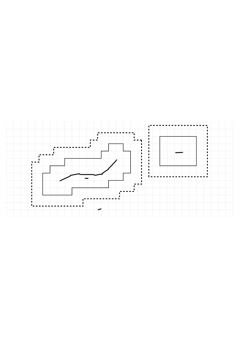
Figure 1. On the left, the family of hypercubes ${q_{z}^{k}}$ with sidelength $2k^{-1}$ that covers $\Omega$. On the right, the zoom on the rectangular subset of $\Omega$ in the picture: the continuous line is the boundary of $\Omega_{g}^{k}$ (this set is on the opposite side with respect to the main part of $J_{u}$), while the dashed one is the boundary of $\widetilde{\Omega}^{k}_{b}$ (which is on the same side of the main part of $J_{u}$). In this theorem we put a different rigid motion on each ${q_{z}^{k}}$ intersecting $\widetilde{\Omega}^{k}_{b}$, while in [18, Theorem 3.1] we put 0 in all $\widetilde{\Omega}^{k}_{b}$.

By (3.2)

$$\#B^{k}\leq C\,\mathcal{H}^{n-1}(J_{u})\,k^{n-1}\theta^{-1}\,,$$ (3.5)

(the presence of constant $C$ is due to the fact that the hypercubes ${Q_{z}^{k}}$ may overlap, at most $4^{n}$ times, as $z$ varies in $B^{k}$) and then

$$\mathcal{L}^{n}\left(\widetilde{\Omega}^{k}_{b}\right)\leq C\,\mathcal{H}^{n-1}(J_{u})\,k^{-1}\,\theta^{-1}\,.$$ (3.6)

Let us apply Proposition 2.3 for any $z\in G^{k}$ taking ${Q_{z}^{k}}$ as $Q$ therein (see also Remark 2.4). Then there exist $\omega_{z}\subset{\tilde{q}_{z}^{k}}$ and $a_{z}\colon{{\mathbb{R}}}^{n}\to{{\mathbb{R}}}^{n}$ affine with $e(a_{z})=0$, such that (we recall directly only the condition corresponding to (2.7), weaker than (2.5), and (2.8))

$$\mathcal{L}^{n}(\omega_{z})\leq ck^{-1}\mathcal{H}^{n-1}(J_{u}\cap{Q_{z}^{k}})\leq c\theta k^{-n}\,,$$ (3.7)

$$\|u-a_{z}\|_{L^{p}({\tilde{q}_{z}^{k}}\setminus\omega_{z})}\leq ck^{-1}\|e(u)\|_{L^{p}({Q_{z}^{k}})}$$ (3.8)

$$\|u-a_{z}\|_{L^{1}({\tilde{q}_{z}^{k}}\setminus\omega_{z})}\leq ck^{-1}\|e(u)\|_{L^{1}({Q_{z}^{k}})}$$ (3.9)

and

$$\begin{split}\int\limits_{{q_{z}^{k}}}|e(v_{z}\ast\varphi_{k})-e(u)\ast\varphi_{k}|^{p}\,\mathrm{d}x\leq c\left(\mathcal{H}^{n-1}(J_{u}\cap{Q_{z}^{k}})\,k^{n-1}\right)^{q}\int\limits_{{Q_{z}^{k}}}|e(u)|^{p}\,\mathrm{d}x\leq c\,\theta^{q}\int\limits_{{Q_{z}^{k}}}|e(u)|^{p}\,\mathrm{d}x\,,\end{split}$$ (3.10)

for $v_{z}:=u\chi_{{\tilde{q}_{z}^{k}}\setminus\omega_{z}}+a_{z}\chi_{\omega_{z}}$ and a suitable $q>0$ depending on $p$ and $n$.

We define

$$\omega^{k}:=\bigcup_{z\in G^{k}}\omega_{z}\,.$$ (3.11)

By (3.7) we have

$$\mathcal{L}^{n}(\omega^{k})\leq ck^{-1}\sum_{z\in G^{k}}\mathcal{H}^{n-1}(J_{u}\cap Q_{z}^{k})\leq c\mathcal{H}^{n-1}(J_{u})\,k^{-1}\,.$$ (3.12)

For every $z\in(2k^{-1})\mathbb{Z}^{n}\cap\Omega$ we employ Proposition 2.2 and let $\tilde{a}_{z}\colon{{\mathbb{R}}}^{n}\to{{\mathbb{R}}}^{n}$ be the affine function with $e(\tilde{a}_{z})=0$ such that (also here we recall directly (2.4))

$$\|u-\tilde{a}_{z}\|_{L^{1}({\tilde{q}_{z}^{k}})}\leq Ck^{-1}|{\mathrm{E}}u|({\tilde{q}_{z}^{k}})\,.$$ (3.13)

We remark that for every $z\in G^{k}$

$$\mathcal{L}^{n}({\tilde{q}_{z}^{k}})\|a_{z}-\tilde{a}_{z}\|_{L^{\infty}({\tilde{q}_{z}^{k}})}\leq Ck^{-1}\Big{(}|{\mathrm{E}}u|(\tilde{q}^{k}_{z})+\|e(u)\|_{L^{1}({Q_{z}^{k}})}\Big{)}\,.$$ (3.14)

Indeed, by (3.9) and (3.13) we get

$$\|a_{z}-\tilde{a}_{z}\|_{L^{1}({\tilde{q}_{z}^{k}}\setminus\omega_{z})}\leq Ck^{-1}\Big{(}|{\mathrm{E}}u|({\tilde{q}_{z}^{k}})+\|e(u)\|_{L^{1}({Q_{z}^{k}})}\Big{)}\,,$$ (3.15)

and then we deduce (3.14) because

$$\mathcal{L}^{n}({\tilde{q}_{z}^{k}})\|a_{z}-\tilde{a}_{z}\|_{L^{\infty}({\tilde{q}_{z}^{k}})}\leq C\|a_{z}-\tilde{a}_{z}\|_{L^{1}({\tilde{q}_{z}^{k}}\setminus\omega_{z})}\,,$$

which follows from Lemma 2.5, since $a_{z}-\tilde{a}_{z}$ is affine and $\mathcal{L}^{n}(\omega_{z})\leq\mathcal{L}^{n}({\tilde{q}_{z}^{k}})/4$ because, by assumption, $\theta<\frac{1}{2c}$ (see also (3.7)).

The approximating functions. Let $G^{k}=(z_{j})_{j\in J}$, so that we order (arbitrarily) the elements of $G^{k}$, and define

$$\widetilde{u}_{k}:=\begin{cases}u\quad&\text{in }\widetilde{\Omega}\setminus\omega^{k}\,,\\ a_{z_{j}}\quad&\text{in }\omega_{z_{j}}\setminus\bigcup_{i<j}\omega_{z_{i}}\,,\end{cases}$$ (3.16)

and

$$u_{k}:=\begin{cases}\widetilde{u}_{k}\ast\varphi_{k}\quad&\text{in }\Omega\setminus\widetilde{\Omega}_{b}^{k}\,,\\ \tilde{a}_{z}\quad&\text{in }{q_{z}^{k}}\cap\widetilde{\Omega}_{b}^{k}\cap\Omega\,,\end{cases}$$ (3.17)

where $z\in\{(2k^{-1})\mathbb{Z}^{n}\colon{q_{z}^{k}}\cap\widetilde{\Omega}_{b}^{k}\neq\emptyset\}$ for $\tilde{a}_{z}$ in (3.17). It is immediate that $u_{k}\in SBV^{p}(\Omega;{{\mathbb{R}}}^{n})\cap L^{\infty}(\Omega;{{\mathbb{R}}}^{n})$, since $u\in BD(\Omega)\subset L^{1}(\Omega;{{\mathbb{R}}}^{n})$, and that $u_{k}\in C^{\infty}(\overline{\Omega}\setminus J_{u_{k}};{{\mathbb{R}}}^{n})\cap W^{m,\infty}(\Omega\setminus J_{u_{k}};{{\mathbb{R}}}^{n})$ for every $m\in{\mathbb{N}}$, since $\widetilde{u}_{k}\ast\varphi_{k}$ is smooth in a neighbourhood of $\Omega\setminus\widetilde{\Omega}_{b}^{k}$. Moreover $J_{u_{k}}$ is closed and included in a finite union of boundaries of $n$-dimensional hypercubes ${q_{z}^{k}}$.

Proof of (3.1c). We have that

$$J_{u_{k}}\subset\overline{\widetilde{\Omega}_{b}^{k}}\,,$$

so the definition (3.3) of $\widetilde{\Omega}_{b}^{k}$ gives

$$J_{u_{k}}\subset\bigcup_{z\in B^{k}}(J_{u_{k}}\cap\overline{Q}^{k}_{z})\,.$$ (3.18)

Notice that for every $\widehat{z}\in B^{k}$ (cf. Figure 1)

$$J_{u_{k}}\cap\overline{Q}^{k}_{\widehat{z}}\subset\partial Q^{k}_{\widehat{z}}\cup\bigcup_{{q_{z}^{k}}\subset Q^{k}_{\widehat{z}}}\partial{q_{z}^{k}}\,,$$

and then

$$\mathcal{H}^{n-1}(J_{u_{k}}\cap\overline{Q}^{k}_{\widehat{z}})\leq Ck^{-(n-1)}\,.$$ (3.19)

for $C$ depending only on $n$. Together with (3.5) and (3.18), (3.19) implies (3.1c).

Proof of (3.1d). In order to prove (3.1d) we estimate the amplitude of the jump in two different sets: the common boundaries between hypercubes of sidelength $2k^{-1}$ included in $\widetilde{\Omega}_{b}^{k}$ (which give the jump of $u_{k}$ included in the interior of $\widetilde{\Omega}_{b}^{k}$) and $\partial\widetilde{\Omega}_{b}^{k}$, which is essentially (up to a $\mathcal{H}^{n-1}$-negligible set) contained in the interior of suitable hypercubes of sidelength $2k^{-1}$, recall (3.4) and see Figure 1.

Let $q^{k}_{z}$ and $q^{k}_{z^{\prime}}$ be included in $\widetilde{\Omega}_{b}^{k}$, with $\mathcal{H}^{n-1}(\partial q^{k}_{z}\cap\partial q^{k}_{z^{\prime}})>0$. Then (3.13) gives

$$\begin{split}\|\tilde{a}_{z}-\tilde{a}_{z^{\prime}}\|_{L^{1}({\tilde{q}_{z}^{k}}\cap\tilde{q}^{k}_{z^{\prime}})}\leq\|u-\tilde{a}_{z}\|_{L^{1}({\tilde{q}_{z}^{k}}\cap\tilde{q}^{k}_{z^{\prime}})}+\|u-\tilde{a}_{z^{\prime}}\|_{L^{1}({\tilde{q}_{z}^{k}}\cap\tilde{q}^{k}_{z^{\prime}})}\leq Ck^{-1}|{\mathrm{E}}u|(\tilde{q}^{k}_{z}\cup\tilde{q}^{k}_{z^{\prime}})\,.\end{split}$$ (3.20)

Being $\tilde{a}_{z}-\tilde{a}_{z^{\prime}}$ affine, we have that (recall Lemma 2.5)

$$\frac{4^{n}}{2}k^{-n}\|\tilde{a}_{z}-\tilde{a}_{z^{\prime}}\|_{L^{\infty}({\tilde{q}_{z}^{k}}\cap\tilde{q}^{k}_{z^{\prime}})}=\mathcal{L}^{n}({\tilde{q}_{z}^{k}}\cap\tilde{q}^{k}_{z^{\prime}})\|\tilde{a}_{z}-\tilde{a}_{z^{\prime}}\|_{L^{\infty}({\tilde{q}_{z}^{k}}\cap\tilde{q}^{k}_{z^{\prime}})}\leq C\|\tilde{a}_{z}-\tilde{a}_{z^{\prime}}\|_{L^{1}({\tilde{q}_{z}^{k}}\cap\tilde{q}^{k}_{z^{\prime}})}\,,$$

and together with (3.20) this gives

$$\begin{split}\int\limits_{\partial q^{k}_{z}\cap\partial q^{k}_{z^{\prime}}}\big{|}[u_{k}]\big{|}\,\mathrm{d}\mathcal{H}^{n-1}&=\int\limits_{\partial q^{k}_{z}\cap\partial q^{k}_{z^{\prime}}}|\tilde{a}_{z}-\tilde{a}_{z^{\prime}}|\,\mathrm{d}\mathcal{H}^{n-1}\leq 2^{n-1}k^{-(n-1)}\|\tilde{a}_{z}-\tilde{a}_{z^{\prime}}\|_{L^{\infty}({\tilde{q}_{z}^{k}}\cap\tilde{q}^{k}_{z^{\prime}})}\\ &\leq C\,|{\mathrm{E}}u|(\tilde{q}^{k}_{z}\cup\tilde{q}^{k}_{z^{\prime}})\,.\end{split}$$

We put together all these contributions, observing that the hypercubes ${\tilde{q}_{z}^{k}}$ are finitely overlapping and ${\tilde{q}_{z}^{k}}\subset\widetilde{\Omega}_{b}^{k}$ if $q^{k}_{z}\subset\widetilde{\Omega}_{b}^{k}$ (cf. Figure 1). We therefore obtain that

$$\int\limits_{{\kern 0.0pt(\widetilde{\Omega}_{b}^{k})}^{\mathrm{o}}}\big{|}[u_{k}]\big{|}\,\mathrm{d}\mathcal{H}^{n-1}\leq C\,|{\mathrm{E}}u|(\widetilde{\Omega}_{b}^{k})\,.$$ (3.21)

Let us now consider a node $z$ such that $q_{z}^{k}\cap\partial\widetilde{\Omega}_{b}^{k}\neq\emptyset$. By definition of $\widetilde{\Omega}_{b}^{k}$ we have that $z\in G^{k}\cap\partial\widetilde{\Omega}_{b}^{k}$. We claim that

$$\|\widetilde{u}_{k}-a_{z}\|_{L^{1}({\tilde{q}_{z}^{k}})}\leq Ck^{-1}\|e(u)\|_{L^{1}(\widetilde{Q}^{k}_{z})}\,.$$ (3.22)

Indeed (3.9) and the fact that $\omega_{z}\subset\omega^{k}$ implies that (recall that $\widetilde{u}_{k}=u$ in ${\tilde{q}_{z}^{k}}\setminus\omega^{k}$ by definition)

$$\|\widetilde{u}_{k}-a_{z}\|_{L^{1}({\tilde{q}_{z}^{k}}\setminus\omega^{k})}\leq Ck^{-1}\|e(u)\|_{L^{1}({Q_{z}^{k}})}\,,$$

and it is proven in [18, equation (3.21)] (the definition of $\widetilde{u}_{k}$ is the same, take in [18, equation (3.21)] the version with $p=1$) that

$$\|\widetilde{u}_{k}-a_{z}\|_{L^{1}({\tilde{q}_{z}^{k}}\cap\omega^{k})}\leq C\,\theta k^{-1}\|e(u)\|_{L^{1}(\widetilde{Q}^{k}_{z})}\,,$$

thus (3.22) is proven.

We now combine (3.22) with (3.14), giving

$$\|a_{z}-\tilde{a}_{z}\|_{L^{1}({\tilde{q}_{z}^{k}})}\leq Ck^{-1}\Big{(}|{\mathrm{E}}u|(\tilde{q}^{k}_{z})+\|e(u)\|_{L^{1}({Q_{z}^{k}})}\Big{)}\,,$$

to get

$$\|\widetilde{u}_{k}-\tilde{a}_{z}\|_{L^{1}({\tilde{q}_{z}^{k}})}\leq Ck^{-1}\Big{(}|{\mathrm{E}}u|(\tilde{q}^{k}_{z})+\|e(u)\|_{L^{1}(\widetilde{Q}^{k}_{z})}\Big{)}\,.$$ (3.23)

It follows that for every $x\in\partial\widetilde{\Omega}_{b}^{k}\cap{q_{z}^{k}}$

$$\begin{split}\big{|}[u_{k}]\big{|}(x)=|u_{k}-\tilde{a}_{z}|(x)&\leq C\|\varphi\|_{L^{\infty}(B_{1})}k^{n}\|\widetilde{u}_{k}-\tilde{a}_{z}\|_{L^{1}(B_{k^{-1}}(x))}\\ &\leq Ck^{n}\|\widetilde{u}_{k}-\tilde{a}_{z}\|_{L^{1}({\tilde{q}_{z}^{k}})}\leq Ck^{n-1}\Big{(}|{\mathrm{E}}u|(\tilde{q}^{k}_{z})+\|e(u)\|_{L^{1}(\widetilde{Q}^{k}_{z})}\Big{)}\,,\end{split}$$

where we used the fact that $\varphi_{k}\ast\tilde{a}_{z}=\tilde{a}_{z}$, being $\varphi$ radial and $\tilde{a}_{z}$ affine. We then conclude

$$\int\limits_{\partial\widetilde{\Omega}_{b}^{k}\cap{q_{z}^{k}}}\big{|}[u_{k}]\big{|}\,\mathrm{d}\mathcal{H}^{n-1}\leq C\Big{(}|{\mathrm{E}}u|(\tilde{q}^{k}_{z})+\|e(u)\|_{L^{1}(\widetilde{Q}^{k}_{z})}\Big{)}\,.$$ (3.24)

Let us sum up over $z\in G^{k}$ such that $\mathcal{H}^{n-1}(\partial\widetilde{\Omega}_{b}^{k}\cap{q_{z}^{k}})>0$, namely over $z\in G^{k}\cap\partial\widetilde{\Omega}_{b}^{k}$. For

$$E_{k}^{1,\Omega}:=\bigcup_{z^{\prime}\in B^{k}}z^{\prime}+(-12k^{-1},12k^{-1})^{n}\,,$$ (3.25)

we have that $\widetilde{\Omega}_{b}^{k}\subset E_{k}^{1,\Omega}$ and that (arguing as done for (3.6))

$$\mathcal{L}^{n}(E_{k}^{1,\Omega})\leq C\,\theta^{-1}\,k^{-1}\mathcal{H}^{n-1}(J_{u})\,.$$ (3.26)

Moreover,

$$\bigcup_{z\in G^{k}\cap\partial\widetilde{\Omega}_{b}^{k}}{\tilde{q}_{z}^{k}}\subset\bigcup_{z^{\prime}\in B^{k}}z^{\prime}+(-6k^{-1},6k^{-1})^{n}\,,\qquad\bigcup_{z\in G^{k}\cap\partial\widetilde{\Omega}_{b}^{k}}\widetilde{Q}^{k}_{z}\subset E_{k}^{1,\Omega}\,.$$

Since the hypercubes ${\tilde{q}_{z}^{k}}$, $\widetilde{Q}^{k}_{z}$ are finitely overlapping, by (3.24) we deduce that

$$\int\limits_{\partial\widetilde{\Omega}_{b}^{k}}\big{|}[u_{k}]\big{|}\,\mathrm{d}\mathcal{H}^{n-1}\leq C\int\limits_{J_{u}}\big{|}[u]\big{|}\,\mathrm{d}\mathcal{H}^{n-1}+C\int\limits_{E_{k}^{1,\Omega}}|e(u)|\,\mathrm{d}x\,.$$ (3.27)

Collecting (3.21) and (3.27) we get (3.1d) (recall the definition of $u_{k}$ and the fact that $\widetilde{\Omega}_{b}^{k}\subset E_{k}^{1,\Omega}$).

Proof of the remaining properties. We notice that our definition of $u_{k}$ differs form that one in [18, Theorem 3.1] only in $\widetilde{\Omega}_{b}^{k}$, since there the approximating functions were set equal to 0. In particular we may employ properties referring to hypercubes in $\Omega\setminus\widetilde{\Omega}_{b}^{k}$ proven in [18, Theorem 3.1].

We set

$$E_{k}^{3,\Omega}:=E_{k}^{1,\Omega}\cup\omega^{k}\,.$$ (3.28)

Then, by (3.11), (3.12), and (3.26), we get immediately that

$$\mathcal{L}^{n}(E_{k}^{3,\Omega})\leq C\,\theta^{-1}\,k^{-1}\mathcal{H}^{n-1}(J_{u})\,.$$ (3.29)

Combining [18, equations (3.15), (3.16), (3.17), (3.21)] we have directly

$$\|u-u_{k}\|_{L^{p}((\Omega\setminus\widetilde{\Omega}_{b}^{k})\setminus\omega^{k})}\leq Ck^{-1}\|e(u)\|_{L^{p}(\widetilde{\Omega})}\,.$$ (3.30)

which implies (3.1f). We may also obtain the above estimate for $p=1$, employing (3.9) in place of (3.8).

Moreover we may follow exactly the argument to prove property (3.1d) in [18], with $\psi=|\cdot|$ and $p=1$ therein (that satisfy $(\mathrm{HP}\psi)$ therein). Replacing $\psi=|\cdot|$ and $p=1$ in [18, equation below (3.25)] and summing over $j$ (that is, over the good nodes) gives, with the notation of [18],

$$\|u-u_{k}\|_{L^{1}((\Omega\setminus\widetilde{\Omega}_{b}^{k})\cap\omega^{k})}\leq Ck^{-1}\|e(u)\|_{L^{1}(\widetilde{\Omega})}+C\theta\|u\|_{L^{1}(\widetilde{\Omega}_{g,2}^{k})}+Ck^{-1/2}\|u\|_{L^{1}(\widetilde{\Omega})}\,.$$ (3.31)

The set $\widetilde{\Omega}_{g,2}^{k}$ above is defined (as in [18]) as follows: we set $G^{k}_{1}$ as the good nodes for which the condition on $J_{u}$ is satisfied for $k^{-\frac{1}{2}}$ in place of $\theta$

$$G^{k}_{1}:=\{z\in G^{k}\colon\mathcal{H}^{n-1}(J_{u}\cap{Q_{z}^{k}})\leq k^{-(n-\frac{1}{2})}\}\,,\qquad G^{k}_{2}:=G^{k}\setminus G^{k}_{1}\,.$$

and the set $\widetilde{G}^{k}_{1}$ of the nodes adjacent to nodes in $G^{k}_{1}$

$$\begin{split}\widetilde{G}^{k}_{1}&:=\{z\in G^{k}\colon\overline{z}\in G^{k}_{1}\text{ for each }\overline{z}\in(2k^{-1}){\mathbb{Z}}^{n}\text{ with }\|z-\overline{z}\|_{\infty}=2k^{-1}\}\,,\\ \widetilde{G}^{k}_{2}&:=\{z\in G^{k}\colon\text{ there exists }\overline{z}\in G^{k}_{2}\text{ with }\|z-\overline{z}\|_{\infty}=2k^{-1}\}\,,\end{split}$$

and then

$$\widetilde{\Omega}^{k}_{g,2}:=\bigcup_{z_{j}\in\widetilde{G}^{k}_{2}}\widetilde{Q}_{z_{j}}\,.$$

We get that $\#G^{2}_{k}\leq\mathcal{H}^{n-1}(J_{u})\,k^{n-\frac{1}{2}}$, so

$$\#\widetilde{G}^{k}_{2}\leq(3^{n}-1)\mathcal{H}^{n-1}(J_{u})\,k^{n-\frac{1}{2}}\,.$$ (3.32)

In order to uniform the notation of the present work, we set

$$E_{k}^{2,\Omega}:=\widetilde{\Omega}^{k}_{g,2}\,.$$

By (3.32) we readily have

$$\mathcal{L}^{n}(E_{k}^{2,\Omega})\leq C\,k^{-\frac{1}{2}}\,\mathcal{H}^{n-1}(J_{u})\,.$$ (3.33)

Furthermore, the definition (3.17) of $u_{k}$ and (3.13) give

$$\|u-u_{k}\|_{L^{1}(\widetilde{\Omega}^{k}_{b})}\leq Ck^{-1}|{\mathrm{E}}u|\big{(}\widetilde{\Omega}^{k}_{b}+(-2k^{-1},2k^{-1})^{n}\big{)}\,.$$ (3.34)

Collecting (3.30) for $p=1$, (3.31), and (3.34), and recalling the definition of $E_{k}^{1,\Omega}$ (3.25), we obtain (3.1e).

Since it is still true (as in [18]) that $e(u_{k})=0$ on $\widetilde{\Omega}_{b}^{k}$ because $e(\tilde{a}_{z})=0$, we get for free (3.1b), that corresponds exactly to [18, eqs. (3.34), (3.35)] summed over $j$ (that is over the good nodes).

We have proven in particular that $u_{k}$ is bounded in $BD(\Omega)$, so the $L^{1}$ convergence of $u_{k}$ to $u$ (guaranteed by (3.1e)) implies (3.1g), and (3.1h) follows immediately from (3.1b) (recall [9, Theorem 1.1]). This concludes the proof. ∎

4. Proof of the main density theorem

Proof of Theorem 1.1.

The proof is quite long and technical, and it is divided in steps for the reader’s convenience.

In the first step we construct a suitable partition of $\Omega$ (up to a negligible set), made by sets whose internal part contains a small jump of $u$. The main part of $J_{u}$ lies on the boundary of some of these subdomains, and is an almost flat interface.

In the second step we define the approximating functions $u_{k}$, starting from the application of Theorem 3.1 in each subdomain; to do so, we have first to extend a little bit outside the restriction of $u$ (indeed Theorem 3.1 requires the original function defined in an enlarged set $\widetilde{\Omega}$), controlling the quantity to approximate (then we employ Lemma 2.1).

The third step is devoted to verify the properties of the approximation. By Theorem 3.1 we deduce directly the estimates on $u_{k}$ outside a set $\widehat{\Gamma}$, which is the main part of $J_{u}$. Then we have to carefully deal with $u_{k}$ on $\widehat{\Gamma}$, in order to show that the jump part of $u_{k}$ is there close to the jump part of $u$.

Let us fix $k\in{\mathbb{N}}$ large enough (the precise conditions will be imposed during the proof).

Step 1. A suitable partition of $\Omega$.

Substep 1.1. Approximation of $J_{u}$ and $\partial\Omega$ and almost covering by hypercubes. We now recall the covering obtained in the first part of [18, Theorem 1.1], referring to that theorem for details. For every $\varepsilon>0$, there exist a finite family of pairwise disjoint closed hypercubes $(\overline{Q_{j}})_{j=1}^{\overline{\jmath}}\subset\Omega$ with

$$\overline{Q_{j}}=\overline{Q}(x_{j},\varrho_{j})\quad\text{for }x_{j}\in J_{u}\,\text{ and one face of $\overline{Q_{j}}$ normal to $\nu_{u}(x_{j})$}\,,$$

$\nu_{u}(x_{j})$ denoting the normal to $J_{u}$ at $x_{j}$, and $C^{1}$ hypersurfaces $(\Gamma_{j})_{j=1}^{\overline{\jmath}}$ with $x_{j}\in\Gamma_{j}$ such that

$$\mathcal{H}^{n-1}\Big{(}J_{u}\setminus\bigcup_{j=1}^{\overline{\jmath}}Q_{j}\Big{)}<\varepsilon\,,$$ (4.1a)

$$\mathcal{H}^{n-1}\big{(}(J_{u}\triangle\Gamma_{j})\,\cap \,\overline{Q_{j}}\big{)}<\varepsilon(2\varrho_{j})^{n-1}<\,\frac{\varepsilon}{1-\varepsilon}\mathcal{H}^{n-1}(J_{u}\cap\overline{Q_{j}})\,,$$ (4.1b)

$$\Gamma_{j}\,\text{is a $C^{1}$ graph with respect} \text{ to }\nu_{u}(x_{j})\text{ with Lipschitz constant less than $\varepsilon/2$}\,.$$ (4.1c)

In particular, (4.1c) gives

$$\Gamma_{j}\subset\Big{\{}x_{j}+\sum_{i=1}^{n-1}y_{i}\,b_{j,i}+y_{n}\,\nu_{u}(x_{j})\colon y_{i}\in(-\varrho_{j},\varrho_{j}),\,y_{n}\in\Big{(}-\frac{\varepsilon\varrho_{j}}{2},+\frac{\varepsilon\varrho_{j}}{2}\Big{)}\Big{\}}\,,$$

where $(b_{j,i})_{i=1}^{n-1}$ is an orthonormal basis of $\nu_{u}(x_{j})^{\perp}$.

Arguing similarly for $\partial\Omega$ in place of $J_{u}$, there exist a finite family of closed hypercubes $(\overline{Q}_{h}^{0})_{h=1}^{\overline{h}}$ of centers $x_{h}^{0}\in\partial\Omega$ and sidelength $2\varrho_{h}^{0}$, with one face normal to $\nu_{\Omega}(x_{h}^{0})$ (the outer normal to $\Omega$ at $x_{h}^{0}$), pairwise disjoint and with empty intersection with any $\overline{Q}_{j}$, and $C^{1}$ hypersurfaces $(\Gamma_{h}^{0})_{h=1}^{\overline{h}}$ with $x_{h}^{0}\in\Gamma_{h}^{0}$, such that

$$\mathcal{H}^{n-1}\Big{(} \partial\Omega\setminus\bigcup_{h=1}^{\overline{h}}Q_{h}^{0}\Big{)}<\varepsilon\,,$$ (4.2a)

$$\mathcal{H}^{n-1}\big{(}(\partial\Omega\triangle\Gamma_{h}^{0})\cap\overline{Q}_{h}^{0}\big{)} <\varepsilon(2\varrho_{h}^{0})^{n-1}<\frac{\varepsilon}{1-\varepsilon}\mathcal{H}^{n-1}(\partial\Omega\cap\overline{Q}_{h}^{0})\,,$$ (4.2b)

$$\Gamma_{h}^{0}\,\text{is a $C^{1}$ graph with respect}\text{ to } \nu_{\Omega}(x_{h}^{0})\text{ with Lipschitz constant less than $\varepsilon/2$}\,.$$ (4.2c)

Notice that we may assume that conditions (4.1) and (4.2) hold also for the enlarged hypercubes

$$\overline{Q}_{j}+(-16\sqrt{n}k^{-1},16\sqrt{n}k^{-1})^{n}\,,\qquad\overline{Q}_{h}^{0}+(-16\sqrt{n}k^{-1},16\sqrt{n}k^{-1})^{n}\,,$$

for $k$ such that $k^{-1}$ is much smaller than $\varepsilon$ and $\min_{j,h}\{\varrho_{j},\varrho_{h}^{0}\}$.

We denote

$$\widehat{\Gamma}:=\bigcup_{j=1}^{\overline{\jmath}}(Q_{j}\cap\Gamma_{j})\,,\qquad\qquad\widehat{\Gamma}_{\partial\Omega}:=\bigcup_{h=1}^{\overline{h}}(Q_{h}^{0}\cap\Gamma_{h}^{0})\,.$$ (4.3)

From (4.1a), (4.1b), and (4.2a), (4.2b) it follows that

$$\mathcal{H}^{n-1}(J_{u}\triangle\widehat{\Gamma})<C\,\varepsilon\,\mathcal{H}^{n-1}(J_{u})\,,\qquad\mathcal{H}^{n-1}(\partial\Omega\triangle\widehat{\Gamma}_{\partial\Omega})<C\,\varepsilon\,\mathcal{H}^{n-1}(\partial\Omega)\,.$$ (4.4)

Let

$$\eta_{\varepsilon}:=\varepsilon\vee\Big{(}\int\limits_{J_{u}\setminus\widehat{\Gamma}}\big{|}[u]\big{|}\,\mathrm{d}\mathcal{H}^{n-1}+\int\limits_{\partial\Omega\setminus\widehat{\Gamma}_{\partial\Omega}}|\mathrm{tr}_{\Omega}u|\,\mathrm{d}\mathcal{H}^{n-1}\Big{)}^{1/(n-1)}\,.$$ (4.5)

Then $\lim_{\varepsilon\to 0}\eta_{\varepsilon}=0$, since $[u]\in L^{1}(J_{u};{{\mathbb{R}}}^{n})$ and $\mathrm{tr}_{\Omega}u\in L^{1}(\partial\Omega;{{\mathbb{R}}}^{n})$, being $\Omega$ Lipschitz and $u\in SBD(\Omega)$. Moreover, we set

$$B_{0}:=\Omega\setminus\Big{(}\bigcup_{j=1}^{\overline{\jmath}}\overline{Q_{j}}\cup\bigcup_{h=0}^{\overline{h}}\overline{Q}_{h}^{0}\Big{)}\,.$$ (4.6)

Substep 1.2. Partition of the hypercubes, almost covering $J_{u}$ and ${\partial\Omega}$, into (almost) hyperrectangles. We fix a single cube in the collection $(\overline{Q_{j}})_{j=1}^{\overline{\jmath}}$ or $(\overline{Q}_{h}^{0})_{h=1}^{\overline{h}}$, we denote it by $\overline{Q}=\overline{Q}(x,\varrho)$ and we call $\Gamma$ the corresponding hypersurface that splits $Q$ in two (almost) half hypercubes $Q^{+}$ and $Q^{-}$, to ease the reading ($\Gamma$ is either close to $J_{u}$ or to $\partial\Omega$). We also assume that $x=0$ and $\nu(x)=e_{n}$ in order to describe the partition of $Q$ that we are going to define.

Figure 2. The hypercubes $Q_{j}$ covering almost all $J_{u}$, the relative (almost) hyperrectangles $Q^{\pm}_{\textbf{m}}$, and the small hypercubes ${q_{z}^{k}}$ partitioning $\Omega$. The $(n{-}1)$-dimensional hypercube which is the “basis” of $Q^{-}_{\textbf{m}}$ is denoted $F_{\textbf{m}}$. The circle represents the zone which is zoomed in Figure 3.

Figure 3. The zoom on the circle in Figure 2: we see the zone between two adjacent (almost) hyperrectangles for a cube $Q_{j}$, oriented with $\nu_{u}(x_{j})$. Notice the different orientation of the hypercubes ${q_{z}^{k}}$, ${\tilde{q}_{z}^{k}}$, ${Q_{z}^{k}}$ with sidelength of order $k^{-1}$, and the fact that the jump between $Q^{-}_{\textbf{m}}$ and $Q^{-}_{{\textbf{m}}+e_{i}}$ is included in $J^{\prime}_{\textbf{m}}$, in turn included in the circle of Figure 2.

Remark 4.1 (Motivation for the partition).

As in the case of the rough approximation in Theorem 3.1, also now a construction finer than the corresponding one in [18] is needed. In [18] one constructs an auxiliary function in a neighbourhood of both the half hypercubes in a single step, employing a unique extension for each half cube: in the strip of height $\varepsilon\varrho$ containing the jump the original function $u$ was replaced employing values of $u$ in the strip of the same size which is immediately below (for $Q^{-}$) or above (for $Q^{+}$). The argument in [18, Theorem 1.1] continues by applying the rough approximation to the auxiliary functions in both the half hypercubes and in $B_{0}$ and gluing simply by characteristic functions. In this way one introduced a further jump, in correspondence to any $Q$, in any intersection between $\partial Q$ and the strip of height $\varepsilon\varrho$ containing $\Gamma$: even if its $\mathcal{H}^{n-1}$-measure is $C\varepsilon\varrho^{n-1}$ (so the total surface of the union of these jumps is less than $C\varepsilon\,\mathcal{H}^{n-1}(J_{u})$), its amplitude is unfortunately not controlled. The idea is now to modify the original function on a strip of height $k^{-1}$ around $\Gamma$ in order to construct the approximation $u_{k}$ in each half cube, since this works well with convolution with kernels supported on $B(0,k^{-1})$. One has to choose carefully the zone where the function is extended from the two sides of $\Gamma$, in order to control the $\mathcal{H}^{n-1}$-measure of the new jump set.

In order to treat, in the subsequent construction at Step 2, also the hypercubes $(Q_{h}^{0})^{\pm}$ (and after for $B_{0}$), that are possibly not included in $\Omega$, we extend $u$ outside $\Omega$ with the value 0.

Let $k\in{\mathbb{N}}$ be much larger than $(\eta_{\varepsilon}\varrho)^{-1}$, and assume to fix the notation that $\eta_{\varepsilon}k\varrho\in{\mathbb{N}}$ (this is always possible, up to slightly modify the sidelengths $\varrho$, keeping the same properties on the hypercubes, in such a way that $\eta_{\varepsilon}\varrho\in\mathbb{Q}$, and then considering a suitable $k\in{\mathbb{N}}$). Let us fix the (almost) half cube $Q^{-}$ and partition $Q^{-}$ into the union of (almost) hyperrectangles, that will be denoted by $Q^{-}_{\textbf{m}}$ in the following (defined in (4.11) below). Analogously, $Q^{+}$ could be partitioned in (almost) hyperrectangles $Q^{+}_{\textbf{m}}$. We denote

$$F_{\textbf{m}}:=\big{\{}(y_{1},\dots,y_{n-1})\in{\mathbb{R}}^{n-1}\colon y_{i}\in(\eta_{\varepsilon}k)^{-1}m_{i}+\big{(}0,(\eta_{\varepsilon}k)^{-1})\big{\}}\quad$$

$$F^{\prime}_{\textbf{m}}:=F_{\textbf{m}}+(-32\sqrt{n}k^{-1},32\sqrt{n}k^{-1})^{n-1}\,,$$

(the choice of the letter $F$ in $F_{\textbf{m}}$ refers to the fact that we consider a “face” of an $n$-dimensional cube), for

$$\textbf{m}=(m_{1},\dots,m_{n-1})\in\{-\eta_{\varepsilon}k\varrho,-\eta_{\varepsilon}k\varrho+1,\dots,0,\dots,\eta_{\varepsilon}k\varrho-1\}^{n-1}\subset{\mathbb{N}}^{n-1}\,.$$ (4.7)

Since $\Gamma$ is the graph of a $\varepsilon/2$-Lipschitz function with respect to $e_{n}$ and $\eta_{\varepsilon}\geq\varepsilon$, there exists $m_{n}\in{\mathbb{R}}$, depending on m, such that

$$\Gamma\cap\big{(}F^{\prime}_{\textbf{m}}{\times}(-\varrho,(\varepsilon\varrho)/2)\big{)}\subset F^{\prime}_{\textbf{m}}{\times}(m_{n},m_{n}+1/2)k^{-1}\,,$$ (4.8)

where $(m_{n},m_{n}+1/2)k^{-1}=(m_{n}k^{-1},(m_{n}+1/2)k^{-1})\subset{\mathbb{R}}$ (indeed every side of $F_{\textbf{m}}$ has length $\eta_{\varepsilon}^{-1}k^{-1}\leq\varepsilon^{-1}k^{-1}$). Let us set

$$u_{\textbf{m}}^{-}:=\begin{dcases}u\quad&\text{in }F^{\prime}_{{\textbf{m}}}{\times}(-\varrho-16\sqrt{n}k^{-1},m_{n}k^{-1})\\ \widehat{u}\quad&\text{in }F^{\prime}_{{\textbf{m}}}{\times}\big{(}(m_{n},m_{n}+25\sqrt{n})k^{-1}\big{)}\,,\end{dcases}$$ (4.9)

where $\widehat{u}$ is obtained by Lemma 2.1 taking $F^{\prime}_{{\textbf{m}}}{\times}\{m_{n}k^{-1}\}$,

$$R_{{\textbf{m}}}:=F^{\prime}_{{\textbf{m}}}{\times}\big{(}(m_{n}-25\sqrt{n},m_{n})k^{-1}\big{)}\,,\qquad R^{\prime}_{{\textbf{m}}}:=F^{\prime}_{{\textbf{m}}}{\times}\big{(}(m_{n},m_{n}+25\sqrt{n})k^{-1}\big{)}$$ (4.10)

as $F$, $R$, $R^{\prime}$ therein, respectively. We introduce (see figures at page 2)

$$Q^{-}_{{\textbf{m}}}:=Q^{-}\cap(F_{{\textbf{m}}}{\times}{\mathbb{R}})\,,\qquad(Q^{-}_{\textbf{m}})^{\prime}:=\Big{(}Q_{{\textbf{m}}}^{-}+(-16\sqrt{n}k^{-1},16\sqrt{n}k^{-1})^{n}\Big{)}\cap(F^{\prime}_{\textbf{m}}{\times}{\mathbb{R}})\,,$$ (4.11)

and

$$Q^{+}_{{\textbf{m}}}:=Q^{+}\cap(F_{{\textbf{m}}}{\times}{\mathbb{R}})\,,\qquad(Q^{+}_{\textbf{m}})^{\prime}:=\Big{(}Q_{{\textbf{m}}}^{+}+(-16\sqrt{n}k^{-1},16\sqrt{n}k^{-1})^{n}\Big{)}\cap(F^{\prime}_{\textbf{m}}{\times}{\mathbb{R}})\,.$$ (4.12)

Notice that $Q_{\textbf{m}}:=Q^{-}_{\textbf{m}}\cup Q^{+}_{\textbf{m}}$ is a hyperrectangle, that coincides with $Q\cap(F_{\textbf{m}}{\times}{\mathbb{R}})$.

Step 2. Definition of the approximating functions.

Substep 2.1. Definition in the (almost) hyperrectangles. We now construct a function $(u_{k})^{-}_{\textbf{m}}$ that approximates $u^{-}_{\textbf{m}}$ in the (almost) hyperrectangle $Q^{-}_{\textbf{m}}$, following the procedure in Theorem 3.1. The set $(Q^{-}_{\textbf{m}})^{\prime}$ has for $Q^{-}_{\textbf{m}}$ the same role that $\widetilde{\Omega}$ has for $\Omega$ in Theorem 3.1 (in the following $\Omega$ is the reference set for Theorem 1.1). We now recall briefly the notation and the construction employed in the proof of Theorem 3.1, for the reader’s convenience.

We introduce for any $z\in(2k^{-1})\mathbb{Z}^{n}\cap\Omega$ the hypercubes ${q_{z}^{k}}$, ${\tilde{q}_{z}^{k}}$, ${Q_{z}^{k}}$, $\widetilde{Q}_{z}^{k}$ with “center” $z$ and sidelength $2k^{-1}$, $4k^{-1}$, $8k^{-1}$, $16k^{-1}$, respectively. We stress that the nodes are fixed once for all in $\Omega$, regardless of the orientation of the cube $Q$ and of $Q_{\textbf{m}}^{\pm}$; we have assumed before that $Q$ is “centered” in 0 and oriented in the vertical direction only to describe the construction of $Q_{\textbf{m}}^{\pm}$. In order to keep the same notation for $Q$, in the following we fix a reference frame in correspondence to $Q$: then we have that in this reference frame the nodes are not anymore in the positions $(2k^{-1})\mathbb{Z}^{n}$ (see Figure 3). Notice that the presence of $\sqrt{n}$ in the sets in (4.10), (4.11) is exactly due to the different orientation between the cube $Q$ and the hypercubes ${q_{z}^{k}}$, ${\tilde{q}_{z}^{k}}$, ${Q_{z}^{k}}$, $\widetilde{Q}^{k}_{z}$.

We look to the (almost) hyperrectangle $Q_{\textbf{m}}^{-}$ (and $(Q^{-}_{\textbf{m}})^{\prime}$) and divide the nodes $z$ inside $Q_{\textbf{m}}^{-}$ into good ones and bad ones, with respect to $u^{-}_{\textbf{m}}$ (in particular with respect to the measure of $J_{u^{-}_{\textbf{m}}}$ in each ${Q_{z}^{k}}$). We then obtain two families $(G^{k})^{-}_{\textbf{m}}$ and $(B^{k})^{-}_{\textbf{m}}$, of good and bad nodes with respect to $u_{\textbf{m}}^{-}$. We consider an enumeration $(G^{k})_{\textbf{m}}^{-}=(z_{j})_{j\in J_{\textbf{m}}^{-}}$ for $(G^{k})^{-}_{\textbf{m}}$, and for each good node $z_{j}$ we employ Proposition 2.3 giving us an infinitesimal rigid motion $(a_{z_{j}})^{-}_{\textbf{m}}$ and an exceptional set $(\omega_{z_{j}})^{-}_{\textbf{m}}$, such that a Korn-Poincaré Inequality holds in $\tilde{q}_{z_{j}}^{k}\setminus(\omega_{z_{j}})^{-}_{\textbf{m}}$ (cf. (3.7)–(3.10)). Moreover, for any node $z$ (good or bad) let $(\tilde{a}_{z})^{-}_{\textbf{m}}$ be the infinitesimal rigid motion provided by the $BD$ Korn-Poincaré Inequality recalled in Proposition 2.2.

Notice that the same node $z$ such that ${Q_{z}^{k}}$ intersects two adjacent (almost) hyperrectangles $Q_{\textbf{m}}^{-}$ and $Q_{{\textbf{m}}+e_{i}}^{-}$ could be at the same time good for $u_{\textbf{m}}^{-}$ and bad for $u_{{\textbf{m}}+e_{i}}^{-}$, or viceversa. We denote

$$(\widetilde{\Omega}_{b}^{k})_{\textbf{m}}^{-}:=\bigcup_{z\in(B^{k})^{-}_{\textbf{m}}}{Q_{z}^{k}}\,,\qquad(\omega^{k})_{\textbf{m}}^{-}:=\bigcup_{z\in(G^{k})_{\textbf{m}}^{-}}(\omega_{z})^{-}_{\textbf{m}}\,,$$ (4.13)

and then we set

$$(\widetilde{u}_{k})_{\textbf{m}}^{-}:=\begin{cases}u^{-}_{\textbf{m}}\quad&\text{in }(Q^{-}_{\textbf{m}})^{\prime}\setminus(\omega^{k})_{\textbf{m}}^{-}\,,\\ (a_{z_{j}})^{-}_{\textbf{m}}\quad&\text{in }(\omega_{z_{j}})^{-}_{\textbf{m}}\setminus\bigcup_{i<j}(\omega_{z_{i}})^{-}_{\textbf{m}}\,,\end{cases}$$ (4.14)

and

$$(u_{k})_{\textbf{m}}^{-}:=\begin{cases}(\widetilde{u}_{k})_{\textbf{m}}^{-}\ast\varphi_{k}\quad&\text{in }Q^{-}_{\textbf{m}}\setminus(\widetilde{\Omega}_{b}^{k})_{\textbf{m}}^{-}\,,\\ (\tilde{a}_{z})^{-}_{\textbf{m}}\quad&\text{in }{q_{z}^{k}}\cap(\widetilde{\Omega}_{b}^{k})_{\textbf{m}}^{-}\cap Q^{-}_{\textbf{m}}\,,\end{cases}$$ (4.15)

We set

$$(E_{k}^{i})^{-}_{\textbf{m}}:=E_{k}^{i,Q^{-}_{\textbf{m}}}\,,\quad\text{for }i\in\{1,2,3\}\,,$$ (4.16)

where $E_{k}^{i,Q^{-}_{\textbf{m}}}\subset(Q^{-}_{\textbf{m}})^{\prime}$ are the exceptional sets provided by Theorem 3.1.

Substep 2.2. Definition in the hypercubes $Q$. We define (assuming that $(u_{k})_{\textbf{m}}^{-}$ is extended arbitrarily outside $Q^{-}_{\textbf{m}}$, otherwise there is a slight abuse of notation in the definition below)

$$(u_{k})_{Q^{-}}:=\sum_{{\textbf{m}}}\chi_{Q^{-}_{{\textbf{m}}}}(u_{k})_{{\textbf{m}}}^{-}\,,$$ (4.17)

We do the analogous construction on $Q^{+}$ to get $(u_{k})_{Q^{+}}$ in $Q^{+}$ (and all the other objects, such as $(u_{k})_{\textbf{m}}^{+}$ or $(E_{k}^{i})_{\textbf{m}}^{+}$, denoted by an apex ⁺ in place of ^-), and then we define the approximating function in $Q$ as (also here, we could assume that $(u_{k})_{Q^{\pm}}$ are defined arbitrarily in $Q^{\pm}$, to avoid an abuse of notation)

$$(u_{k})_{Q}:=\chi_{Q^{-}}\,(u_{k})_{Q^{-}}+\chi_{Q^{+}}\,(u_{k})_{Q^{+}}\,.$$ (4.18)

We define

$$(E_{k}^{i})_{Q}^{\pm}:=\bigcup_{\textbf{m}}(E_{k}^{i})_{\textbf{m}}^{\pm}\,,\quad\text{for }i\in\{1,2,3\}\,,$$ (4.19)

and eventually, $(E_{k}^{i})_{Q}:=(E_{k}^{i})_{Q}^{+}\cup(E_{k}^{i})_{Q}^{-}$.

Substep 2.3. Definition of the approximating functions in $\Omega$. We consider $\widetilde{B}_{0}:=B_{0}+(-16\sqrt{n}k^{-1},16\sqrt{n}k^{-1})^{n}$ and we denote $(u_{k})_{B_{0}}$ the $k$-th approximating function for $u$ given by Theorem 3.1 (arguing as described before for $Q^{-}_{\textbf{m}}$) in correspondence to $B_{0}$, starting from the extension of $u$ with value 0 outside $\Omega$, in $\widetilde{B}_{0}$. Then we define the global $k$-th approximating function

$$u_{k}:=\chi_{B_{0}}(u_{k})_{B_{0}}+\sum_{j=1}^{\overline{\jmath}}\chi_{Q_{j}}(u_{k})_{Q_{j}}+\sum_{h=1}^{\overline{h}}\chi_{Q_{h}^{0}\cap\Omega}(u_{k})_{Q_{h}^{0}}\,.$$ (4.20)

We denote

$$E_{k}^{i}:=E_{k}^{i,B_{0}}\cup\bigcup_{Q}(E_{k}^{i})_{Q}\,,\quad\text{for }i\in\{1,2,3\}\,,$$

where $E_{k}^{i,B_{0}}$ are the exceptional sets by Theorem 3.1 for $B_{0}$. It is easy to see (recall (3.1a) and (3.1f) and notice that after the extension process of Lemma 2.1 the measure of the exceptional sets is still controlled) that

$$\mathcal{L}^{n}(E^{1}_{k})+\mathcal{L}^{n}(E^{3}_{k})\leq C\,k^{-1}\,,\qquad\mathcal{L}^{n}(E^{2}_{k})\leq C\,k^{-\frac{1}{2}}\,.$$ (4.21)

Step 3. Properties of the approximating functions.

Substep 3.1. Direct consequences of Theorem 3.1. We observe that, by Theorem 3.1, $J_{(u_{k})^{\pm}_{\textbf{m}}}$ is closed and included in a finite union of boundaries of $n$-dimensional hypercubes (the bad hypercubes and the boundary good hypercubes), and $(u_{k})_{\textbf{m}}^{\pm}$ is smooth outside its jump set up to the boundary of $Q^{\pm}_{\textbf{m}}$. Therefore, by (4.18), $J_{(u_{k})_{Q}}$ is closed and included in $\bigcup_{\textbf{m}}(J_{(u_{k})_{\textbf{m}}}\cup\partial Q^{-}_{\textbf{m}}\cup\partial Q^{+}_{\textbf{m}})$ (we will see below that it is enough to take $\Gamma$ and the small sets $J^{\prime}_{\textbf{m}}$, see (4.29), instead of the union of all $\partial Q^{\pm}_{\textbf{m}}$).

Moreover, $(u_{k})_{Q}\in SBV(Q;{{\mathbb{R}}}^{n})\cap C^{\infty}(\overline{Q}\setminus J_{(u_{k})_{Q}};{{\mathbb{R}}}^{n})\cap W^{m,\infty}(Q\setminus J_{(u_{k})_{Q}};{{\mathbb{R}}}^{n})$ for every $m\in{\mathbb{N}}$, since this holds separately for each $(u_{k})^{\pm}_{\textbf{m}}$ up to the boundary of $Q^{\pm}_{\textbf{m}}$.

In the same way, looking at (4.20), $u_{k}\in SBV(\Omega;{{\mathbb{R}}}^{n})\cap C^{\infty}(\overline{\Omega}\setminus J_{u_{k}};{{\mathbb{R}}}^{n})\cap W^{m,\infty}(\Omega\setminus J_{u_{k}};{{\mathbb{R}}}^{n})$ for every $m\in{\mathbb{N}}$, $J_{u_{k}}$ is closed and

$$J_{u_{k}}\subset J_{(u_{k})_{B^{0}}}\cup\bigcup_{Q}(J_{(u_{k})_{Q}}\cup\partial Q)$$

(where $Q$ stands for all the $Q_{j}$ and $Q_{h}^{0}$) which is a finite union of $C^{1}$ hypersurfaces (we will see below that it is enough to take just a little part of $\partial Q$, see (4.34)).

For any m, Lemma 2.1 gives (as usual we omit the target sets ${{\mathbb{R}}}^{n}$ and ${\mathbb{M}^{n\times n}_{sym}}$ in the notation for the $L^{1}$ norm of $u$ and $e(u)$, and we argue to fix the ideas in $Q_{\textbf{m}}^{-}$)

$$\|u_{{\textbf{m}}}^{-}\|_{L^{1}(R^{\prime}_{{\textbf{m}}})} \leq C\|u\|_{L^{1}(R_{\textbf{m}})}\,,$$ (4.22a)

$$\|e(u_{{\textbf{m}}}^{-})\|_{L^{p}(R^{\prime}_{{\textbf{m}}})} \leq C\|e(u)\|_{L^{p}(R_{\textbf{m}})}\,,$$ (4.22b)

$$\mathcal{H}^{n-1}(J_{u_{{\textbf{m}}}^{-}}\cap R^{\prime}_{{\textbf{m}}}) \leq C\mathcal{H}^{n-1}(J_{u}\cap R_{{\textbf{m}}})\,,$$ (4.22c)

$$\int\limits_{R^{\prime}_{{\textbf{m}}}}\big{|}[u_{{\textbf{m}}}^{-}]\big{|}\,\mathrm{d}\mathcal{H}^{n-1} \leq C\int\limits_{R_{{\textbf{m}}}}\big{|}[u]\big{|}\,\mathrm{d}\mathcal{H}^{n-1}\,.$$ (4.22d)

We now employ the properties stated in Theorem 3.1 (we take $\theta$ fixed, so we absorb it in $C$).

By (3.1b) we have that

$$\begin{split}\int\limits_{Q^{-}_{\textbf{m}}}|e((u_{k})^{-}_{\textbf{m}})|^{p}\,\mathrm{d}x&\leq(1+C\,k^{-q})\int\limits_{(Q^{-}_{\textbf{m}})^{\prime}}|e(u^{-}_{\textbf{m}})|^{p}\,\mathrm{d}x+C\int\limits_{(E_{k}^{2})^{-}_{\textbf{m}}}|e(u^{-}_{\textbf{m}})|^{p}\,\mathrm{d}x\\ &\leq(1+C\,k^{-q})\int\limits_{(Q^{-}_{\textbf{m}})^{\prime}\setminus R^{\prime}_{\textbf{m}}}|e(u)|^{p}\,\mathrm{d}x+C\int\limits_{(E_{k}^{2})^{-}_{\textbf{m}}\setminus R^{\prime}_{\textbf{m}}}|e(u)|^{p}\,\mathrm{d}x\,,\end{split}$$

where in the last inequality we have employed (4.22). We can argue analogously for $Q^{+}_{\textbf{m}}$, employ (3.1b) for $B_{0}$, and sum all the inequalities, to get

$$\begin{split}\int\limits_{\Omega}|e(u_{k})|^{p}\,\mathrm{d}x&\leq(1+C\,k^{-q})\int\limits_{\Omega}|e(u)|^{p}\,\mathrm{d}x+C\int\limits_{E_{k}^{2}}|e(u)|^{p}\,\mathrm{d}x+C\int\limits_{E^{4}_{k}}|e(u)|^{p}\,\mathrm{d}x\,,\end{split}$$ (4.23a)

where

$$E^{4}_{k}:=\bigcup_{m}(\partial Q^{-}_{\textbf{m}}\cup\partial Q^{+}_{\textbf{m}})+(-16\sqrt{n}k^{-1},16\sqrt{n}k^{-1})^{n}\,.$$

Notice that the contribution on $$E^{4}_{k} (Q^{-}_{\textbf{m}})^{\prime} \Omega$$ comes from the fact that in the right hand side of the estimates we have the enlarged set , then we have superposition of (at most two) adjacent elements of the partition of . Moreover, we have that

$$\mathcal{L}^{n}(E^{4}_{k})\leq C\,k^{-1}\,.$$ (4.23b)

We can argue exactly in the same way employing (3.1e) in place of (3.1b). In $Q^{-}_{\textbf{m}}$ we obtain

$$\begin{split}\int\limits_{Q^{-}_{\textbf{m}}}|u^{-}_{\textbf{m}}-(u_{k})^{-}_{\textbf{m}}|\,\mathrm{d}x&\leq C\,k^{-1}\int\limits_{(Q^{-}_{\textbf{m}})^{\prime}}|e(u^{-}_{\textbf{m}})|\,\mathrm{d}x+C\,k^{-1}|{\mathrm{E}}u^{-}_{\textbf{m}}|((E_{k}^{1})^{-}_{\textbf{m}})+C\int\limits_{(E_{k}^{2})^{-}_{\textbf{m}}}|u^{-}_{\textbf{m}}|\,\mathrm{d}x\\ &\hskip 9.00002pt+C\,k^{-\frac{1}{2}}\int\limits_{(Q^{-}_{\textbf{m}})^{\prime}}|u^{-}_{\textbf{m}}|\,\mathrm{d}x\\ &\leq C\,k^{-1}\int\limits_{(Q^{-}_{\textbf{m}})^{\prime}\setminus R^{\prime}_{\textbf{m}}}|e(u)|\,\mathrm{d}x+C\,k^{-1}|{\mathrm{E}}u|((E_{k}^{1})^{-}_{\textbf{m}}\setminus R^{\prime}_{\textbf{m}})+C\int\limits_{(E_{k}^{2})^{-}_{\textbf{m}}\setminus R^{\prime}_{\textbf{m}}}|u|\,\mathrm{d}x\\ &\hskip 9.00002pt+C\,k^{-\frac{1}{2}}\int\limits_{(Q^{-}_{\textbf{m}})^{\prime}\setminus R^{\prime}_{\textbf{m}}}|u|\,\mathrm{d}x\,,\end{split}$$

and summing over all the contributions we get

$$\begin{split}\int\limits_{\Omega}|u-u_{k}|\,\mathrm{d}x&\leq C\,k^{-1}\int\limits_{\Omega}|e(u)|\,\mathrm{d}x+C\,k^{-1}|{\mathrm{E}}u|(E^{1}_{k}\setminus(\widehat{\Gamma}\cup\widehat{\Gamma}_{\partial\Omega}))+C\int\limits_{E^{2}_{k}}|u|\,\mathrm{d}x\\ &\hskip 9.00002pt+Ck^{-\frac{1}{2}}\int\limits_{\Omega}|u|\,\mathrm{d}x+Ck^{-\frac{1}{2}}\int\limits_{E^{4}_{k}}(|u|+|e(u)|)\,\mathrm{d}x\end{split}$$ (4.24)

Furthermore, starting from (3.1f) in $Q^{-}_{\textbf{m}}$, with a similar procedure we find that

$$\int\limits_{\Omega\setminus E^{3}_{k}}|u-u_{k}|^{p}\,\mathrm{d}x\leq C\,k^{-p}\int\limits_{\Omega}|e(u)|^{p}\,\mathrm{d}x\,.$$ (4.25)

Let us now employ (3.1c) and (3.1d), the two estimates in Theorem 3.1 concerning the jump of the approximating sequences. In any $Q^{-}_{\textbf{m}}$ these give (always recalling (4.22))

$$\mathcal{H}^{n-1}(J_{(u_{k})^{-}_{\textbf{m}}}\cap Q^{-}_{\textbf{m}})\leq C\mathcal{H}^{n-1}(J_{u_{\textbf{m}}}\cap(Q^{-}_{\textbf{m}})^{\prime})\leq C\mathcal{H}^{n-1}(J_{u}\cap(Q^{-}_{\textbf{m}})^{\prime}\setminus R^{\prime}_{\textbf{m}})\,,$$ (4.26a)

and

$$\begin{split}\int\limits_{J_{(u_{k})^{-}_{\textbf{m}}}\cap Q^{-}_{\textbf{m}}}\big{|}[(u_{k})^{-}_{\textbf{m}}]\big{|}\,\mathrm{d}\mathcal{H}^{n-1}&\leq C\int\limits_{J_{u^{-}_{\textbf{m}}}\cap(Q^{-}_{\textbf{m}})^{\prime}}\big{|}[u^{-}_{\textbf{m}}]\big{|}\,\mathrm{d}\mathcal{H}^{n-1}+C\int\limits_{(E_{k}^{1})^{-}_{\textbf{m}}}|e(u^{-}_{\textbf{m}})|\,\mathrm{d}x\\ &\leq C\int\limits_{J_{u}\cap(Q^{-}_{\textbf{m}})^{\prime}\setminus R^{\prime}_{\textbf{m}}}\big{|}[u]\big{|}\,\mathrm{d}\mathcal{H}^{n-1}+C\int\limits_{(E_{k}^{1})^{-}_{\textbf{m}}\setminus R^{\prime}_{\textbf{m}}}|e(u)|\,\mathrm{d}x\,.\end{split}$$ (4.26b)

Notice that for the (almost) half hypercubes $(Q_{h}^{0})^{\pm}$ we have to consider also the possible jump due to the fact that we have extended $u$ outside $\Omega$ with 0, so we could have created jump on $\partial\Omega\setminus\Gamma_{h}^{0}$. So the two estimates above include also in the right hand sides the two terms

$$C\mathcal{H}^{n-1}(((Q_{h}^{0})^{-}_{\textbf{m}})^{\prime}\cap\partial\Omega\setminus\Gamma_{h}^{0})\,,\quad\text{and}\qquad C\int\limits_{((Q_{h}^{0})^{-}_{\textbf{m}})^{\prime}\cap\partial\Omega\setminus\Gamma_{h}^{0}}|\mathrm{tr}_{\Omega}u|\,\mathrm{d}\mathcal{H}^{n-1}\,,$$

respectively. Summing over all the contributions, we estimate (recall (4.1b), (4.4), and (4.5))

$$\mathcal{H}^{n-1}(J_{u_{k}}\setminus H_{k})\leq C\mathcal{H}^{n-1}(J_{u}\setminus\widehat{\Gamma})+C\mathcal{H}^{n-1}({\partial\Omega}\setminus\widehat{\Gamma}_{\partial\Omega})\leq C\varepsilon\big{(}\mathcal{H}^{n-1}(J_{u})+\mathcal{H}^{n-1}({\partial\Omega})\big{)}$$ (4.27a)

and

$$\int\limits_{J_{u_{k}}\setminus H_{k}}\big{|}[u_{k}]\big{|}\,\mathrm{d}\mathcal{H}^{n-1}\leq C\int\limits_{J_{u}\setminus\widehat{\Gamma}}\big{|}[u]\big{|}\,\mathrm{d}\mathcal{H}^{n-1}+C\int\limits_{\partial\Omega\setminus\widehat{\Gamma}_{\partial\Omega}}|\mathrm{tr}_{\Omega}u|\,\mathrm{d}\mathcal{H}^{n-1}\leq C\eta_{\varepsilon}^{n-1}\,,$$ (4.27b)

where

$$H_{k}:=\bigcup_{Q}\bigcup_{\textbf{m}}(\partial Q^{-}_{\textbf{m}}\cup\partial Q^{+}_{\textbf{m}})\,.$$

Substep 3.2. Estimate of the jump part.

Substep 3.2.1. Estimate of $\mathcal{H}^{n-1}(J_{u_{k}})$ outside $\widehat{\Gamma}\cup\widehat{\Gamma}_{{\partial\Omega}}$. Let us examine the jump for $(u_{k})_{Q^{-}}$ created on the common boundaries between two sets $Q^{-}_{\textbf{m}}$, $Q^{-}_{{\textbf{m}}^{\prime}}$, namely between two sets $Q^{-}_{\textbf{m}}$ and $Q^{-}_{{\textbf{m}}\pm e_{i}}$ for $i=1,\dots,{n-1}$, both inside $Q^{-}$. To fix the ideas let us take m and consider $Q^{-}_{\textbf{m}}$ and $Q^{-}_{{\textbf{m}}+e_{i}}$. Notice that

$$|m_{n}({\textbf{m}})-m_{n}({\textbf{m}}+e_{i})|\leq 1/2\,,$$

where $m_{n}({\textbf{m}})k^{-1}$ and $m_{n}({\textbf{m}}+e_{i})k^{-1}$ are the “heights” corresponding to $Q^{-}_{\textbf{m}}$ and $Q^{-}_{{\textbf{m}}+e_{i}}$, see (4.8). This means that, for $m_{n}=m_{n}({\textbf{m}})$,

$$\begin{split}u^{-}_{\textbf{m}}&=u\text{ in }F^{\prime}_{{\textbf{m}}}{\times}(-\varrho-16\sqrt{n}k^{-1},(m_{n}-1/2)k^{-1})\,,\\ u^{-}_{{\textbf{m}}+e_{i}}&=u\text{ in }F^{\prime}_{{\textbf{m}}+e_{i}}{\times}(-\varrho-16\sqrt{n}k^{-1},(m_{n}-1/2)k^{-1})\,.\end{split}$$

By construction of $(u_{k})^{-}_{\textbf{m}}$ (see (4.14) and (4.15)) we have that

$$(\widetilde{u}_{k})^{-}_{\textbf{m}}=(\widetilde{u}_{k})^{-}_{{\textbf{m}}+e_{i}}\,\text{ in }(F^{\prime}_{\textbf{m}}\cap F^{\prime}_{{\textbf{m}}+e_{i}}){\times}(-\varrho-16\sqrt{n}k^{-1},(m_{n}-(4\sqrt{n}+1/2)k^{-1})\,,$$ (4.28)

and

$$(u_{k})^{-}_{\textbf{m}}=(u_{k})^{-}_{{\textbf{m}}+e_{i}}\,\text{ in }(F^{\prime}_{\textbf{m}}\cap F^{\prime}_{{\textbf{m}}+e_{i}}){\times}(-\varrho-16\sqrt{n}k^{-1},(m_{n}-(8\sqrt{n}+1/2)k^{-1})\,,$$

since, if $x\in{q_{z}^{k}}$, $(\widetilde{u}_{k})^{-}_{\textbf{m}}(x)$ and $(u_{k})^{-}_{\textbf{m}}(x)$ depend only on $u^{-}_{\textbf{m}}$ in ${\tilde{q}_{z}^{k}}$ and ${Q_{z}^{k}}$, respectively (see figure on the right at page 2).

Setting

$$J_{(u_{k})_{Q^{-}}}\cap\partial Q^{-}_{\textbf{m}}\cap\partial Q^{-}_{{\textbf{m}}+e_{i}}=:J^{\prime}_{\textbf{m}}\,,$$ (4.29)

it follows that

$$J^{\prime}_{\textbf{m}}\subset(\partial F_{\textbf{m}}\cap\partial F_{{\textbf{m}}+e_{i}}){\times}\big{(}(m_{n}-(8\sqrt{n}+1/2),m_{n}+1)k^{-1}\big{)}$$ (4.30)

and thus

$$\mathcal{H}^{n-1}(J^{\prime}_{\textbf{m}})\leq C\eta_{\varepsilon}^{-(n-2)}k^{-(n-1)}\,.$$ (4.31)

Summing up over all the faces of $Q^{-}_{\textbf{m}}$ in the directions $e_{1},\dots,e_{n-1}$ we get

$$\mathcal{H}^{n-1}(J_{(u_{k})_{Q^{-}}}\cap\partial Q^{-}_{\textbf{m}})\leq C\eta_{\varepsilon}^{-(n-2)}k^{-(n-1)}\,;$$ (4.32)

summing up over m gives (see (4.7))

$$\mathcal{H}^{n-1}\Big{(}J_{(u_{k})_{Q^{-}}}\cap\bigcup_{\textbf{m}}\partial Q^{-}_{\textbf{m}}\setminus\partial Q^{-}\Big{)}\leq C\eta_{\varepsilon}\varrho^{n-1}\,.$$ (4.33)

In the very same way we get

$$\mathcal{H}^{n-1}(J_{u_{k}}\cap\partial Q_{j})\leq C\eta_{\varepsilon}^{-(n-2)}k^{-(n-1)}\,,\quad\mathcal{H}^{n-1}(J_{u_{k}}\cap\partial Q_{h}^{0}\cap\Omega)\leq C\eta_{\varepsilon}^{-(n-2)}k^{-(n-1)}\,.$$ (4.34)

Now we sum (4.33) and (4.34) over $Q=Q_{j}$ or $Q=Q_{h}^{0}$, recalling (4.1b), and add (4.27a): we get

$$\mathcal{H}^{n-1}\big{(}J_{u_{k}}\setminus(\widehat{\Gamma}\cup\widehat{\Gamma}_{\partial\Omega}))\leq C\big{(}\mathcal{H}^{n-1}(J_{u}\setminus\widehat{\Gamma})+\mathcal{H}^{n-1}(\partial\Omega\setminus\widehat{\Gamma}_{\partial\Omega})\big{)}+C\,\big{(}\mathcal{H}^{n-1}(J_{u})+\mathcal{H}^{n-1}(\partial\Omega)\big{)}\,\eta_{\varepsilon}\,.$$ (4.35)

Substep 3.2.2. Estimate of $[u_{k}]_{L^{1}(J_{u_{k}})}$ outside $\widehat{\Gamma}\cup\widehat{\Gamma}_{{\partial\Omega}}$. We now estimate the $L^{1}$ norm of jump amplitude on $J^{\prime}_{\textbf{m}}$, that is on the common boundary between any $Q^{-}_{\textbf{m}}$ and $Q^{-}_{{\textbf{m}}+e_{i}}$, by (4.29). For every $x\in J^{\prime}_{\textbf{m}}$ we may have four cases, depending if $x\in(\widetilde{\Omega}_{b}^{k})^{-}_{\textbf{m}}$, $x\in(\widetilde{\Omega}_{b}^{k})^{-}_{{\textbf{m}}+e_{i}}$, or not, where $(\widetilde{\Omega}_{b}^{k})^{-}_{\textbf{m}}$ is the set of (neighbourhoods of) bad hypercubes corresponding to $(Q^{-}_{\textbf{m}})^{\prime}$, see (4.13).
Case 1. Estimate for the points not in $(\widetilde{\Omega}_{b}^{k})^{-}_{\textbf{m}}\cup(\widetilde{\Omega}_{b}^{k})^{-}_{{\textbf{m}}+e_{i}}$. By construction of $(u_{k})^{-}_{\textbf{m}}$ it follows that

$$[(u_{k})_{Q^{-}}]=\varphi_{k}\ast\big{(}(\widetilde{u}_{k})^{-}_{\textbf{m}}-(\widetilde{u}_{k})^{-}_{{\textbf{m}}+e_{i}}\big{)}\quad\text{in }J^{\prime}_{\textbf{m}}\setminus\big{(}(\widetilde{\Omega}_{b}^{k})^{-}_{\textbf{m}}\cup(\widetilde{\Omega}_{b}^{k})^{-}_{{\textbf{m}}+e_{i}}\big{)}\,,$$

so, for every $x$ in the set above,

$$\big{|}[(u_{k})_{Q^{-}}]\big{|}\leq\|\varphi\|_{L^{\infty}(B_{1})}k^{n}\|(\widetilde{u}_{k})^{-}_{\textbf{m}}-(\widetilde{u}_{k})^{-}_{{\textbf{m}}+e_{i}}\|_{L^{1}(J^{\prime}_{\textbf{m}}+B(0,k^{-1}))}\,.$$ (4.36)

We claim that (see (4.10) for the definition of $R_{\textbf{m}}$)

$$\|(\widetilde{u}_{k})^{-}_{\textbf{m}}-(\widetilde{u}_{k})^{-}_{{\textbf{m}}+e_{i}}\|_{L^{1}(J^{\prime}_{\textbf{m}}+B(0,k^{-1}))}\leq Ck^{-1}|{\mathrm{E}}u|(R_{\textbf{m}}\cap R_{{\textbf{m}}+e_{i}})\,.$$ (4.37)

We have

$$\begin{split}\|(&\widetilde{u}_{k})^{-}_{\textbf{m}}-(\widetilde{u}_{k})^{-}_{{\textbf{m}}+e_{i}}\|_{L^{1}(J^{\prime}_{\textbf{m}}+B(0,k^{-1}))}\leq\sum_{{q_{z}^{k}}\cap(J^{\prime}_{\textbf{m}}+B(0,k^{-1}))\neq\emptyset}\|(\widetilde{u}_{k})^{-}_{\textbf{m}}-(\widetilde{u}_{k})^{-}_{{\textbf{m}}+e_{i}}\|_{L^{1}({q_{z}^{k}})}\\ &\leq\sum_{{q_{z}^{k}}\cap(J^{\prime}_{\textbf{m}}+B(0,k^{-1}))\neq\emptyset}\|(\tilde{a}_{z})^{-}_{{\textbf{m}}}-(\tilde{a}_{z})^{-}_{{\textbf{m}}+e_{i}}\|_{L^{1}({q_{z}^{k}})}+Ck^{-1}\sum_{{q_{z}^{k}}\cap(J^{\prime}_{\textbf{m}}+B(0,k^{-1}))\neq\emptyset}(|{\mathrm{E}}(u^{-}_{\textbf{m}})|(\widetilde{Q}^{k}_{z})+|{\mathrm{E}}(u^{-}_{{\textbf{m}}+e_{i}})|(\widetilde{Q}^{k}_{z}))\end{split}$$ (4.38)

where $(\tilde{a}_{z})^{-}_{\textbf{m}}$ is affine with $e((\tilde{a}_{z})^{-}_{\textbf{m}})=0$ and

$$\|u^{-}_{\textbf{m}}-(\tilde{a}_{z})^{-}_{\textbf{m}}\|_{L^{1}({\tilde{q}_{z}^{k}})}\leq Ck^{-1}|{\mathrm{E}}u^{-}_{\textbf{m}}|({\tilde{q}_{z}^{k}})\,.$$

The second inequality in (4.38) comes from (recall (4.13))

$$\|(\widetilde{u}_{k})^{-}_{\textbf{m}}-(\tilde{a}_{z})^{-}_{\textbf{m}}\|_{L^{1}(q_{j}\setminus(\omega^{k})^{-}_{\textbf{m}})}=\|u^{-}_{\textbf{m}}-(\tilde{a}_{z})^{-}_{\textbf{m}}\|_{L^{1}({q_{z}^{k}}\setminus(\omega^{k})^{-}_{\textbf{m}})}\leq Ck^{-1}|{\mathrm{E}}(u^{-}_{\textbf{m}})|({\tilde{q}_{z}^{k}})\,,$$

and the fact that, recalling (3.23),

$$\|(\widetilde{u}_{k})^{-}_{\textbf{m}}-(\tilde{a}_{z})^{-}_{\textbf{m}}\|_{L^{1}({q_{z}^{k}}\cap(\omega^{k})^{-}_{\textbf{m}})}\leq Ck^{-1}\big{(}|{\mathrm{E}}(u^{-}_{\textbf{m}})|({q_{z}^{k}})+\|e(u^{-}_{\textbf{m}})\|_{L^{1}(\widetilde{Q}^{k}_{z})}\big{)}\,,$$

the same being true for ${\textbf{m}}+e_{i}$ in place of m.

We now estimate $\|(\tilde{a}_{z})^{-}_{{\textbf{m}}}-(\tilde{a}_{z})^{-}_{{\textbf{m}}+e_{i}}\|_{L^{1}({q_{z}^{k}})}$ for ${q_{z}^{k}}\cap(J^{\prime}_{\textbf{m}}+B(0,k^{-1}))\neq\emptyset$ in (4.38). We remark that

$$\mathcal{L}^{n}({\tilde{q}_{z}^{k}}\cap R_{\textbf{m}}\cap R_{{\textbf{m}}+e_{i}})/\mathcal{L}^{n}({\tilde{q}_{z}^{k}})\geq C_{0}>0\,,$$

with $C_{0}$ depending only on $n$. Thus

$$\begin{split}\|(\tilde{a}_{z})^{-}_{{\textbf{m}}}-(\tilde{a}_{z})^{-}_{{\textbf{m}}+e_{i}}\|_{L^{1}({q_{z}^{k}})}&\leq C\|(\tilde{a}_{z})^{-}_{{\textbf{m}}}-(\tilde{a}_{z})^{-}_{{\textbf{m}}+e_{i}}\|_{L^{1}({\tilde{q}_{z}^{k}}\cap R_{\textbf{m}}\cap R_{{\textbf{m}}+e_{i}})}\\ &\leq Ck^{-1}(|{\mathrm{E}}(u^{-}_{\textbf{m}})|(\widetilde{Q}^{k}_{z})+|{\mathrm{E}}(u^{-}_{{\textbf{m}}+e_{i}})|(\widetilde{Q}^{k}_{z}))\,,\end{split}$$ (4.39)

since $(\tilde{a}_{z})^{-}_{{\textbf{m}}}-(\tilde{a}_{z})^{-}_{{\textbf{m}}+e_{i}}$ is an affine function (see Lemma 2.5, in particular the constant in the first inequality above depends on $C_{0}$) and $u^{-}_{\textbf{m}}=u^{-}_{{\textbf{m}}+e_{i}}=u$ in $R_{\textbf{m}}\cap R_{{\textbf{m}}+e_{i}}$. Therefore (4.37) is proven, recalling also (4.22).
Cases 2,3. Points in $(\widetilde{\Omega}_{b}^{k})^{-}_{{\textbf{m}}}\setminus(\widetilde{\Omega}_{b}^{k})^{-}_{{\textbf{m}}+e_{i}}$ or in $(\widetilde{\Omega}_{b}^{k})^{-}_{{\textbf{m}}+e_{i}}\setminus(\widetilde{\Omega}_{b}^{k})^{-}_{\textbf{m}}$. Consider now the case when $x\in J^{\prime}_{\textbf{m}}\cap(\widetilde{\Omega}_{b}^{k})^{-}_{\textbf{m}}$. To fix the ideas assume that $x\in{q_{z}^{k}}$ (in the open cube). So (recall (4.15))

$$(u_{k})^{-}_{\textbf{m}}(x)=(\tilde{a}_{z})^{-}_{\textbf{m}}(x)\,,\quad\text{with }\|u^{-}_{\textbf{m}}-(\tilde{a}_{z})^{-}_{\textbf{m}}\|_{L^{1}({\tilde{q}_{z}^{k}})}\leq Ck^{-1}|{\mathrm{E}}(u^{-}_{\textbf{m}})|({\tilde{q}_{z}^{k}})\,.$$

If $x\notin(\widetilde{\Omega}_{b}^{k})^{-}_{{\textbf{m}}+e_{i}}$, $(u_{k})^{-}_{{\textbf{m}}+e_{i}}(x)=\varphi_{k}\ast(\widetilde{u}_{k})^{-}_{{\textbf{m}}+e_{i}}$, so

$$[(u_{k})_{Q^{-}}](x)=\varphi_{k}\ast\big{(}(\widetilde{u}_{k})^{-}_{{\textbf{m}}+e_{i}}-(\tilde{a}_{z})^{-}_{\textbf{m}}\big{)}(x)\,.$$

Now

$$\begin{split}\|(&\widetilde{u}_{k})^{-}_{{\textbf{m}}+e_{i}}-(\tilde{a}_{z})^{-}_{\textbf{m}}\|_{L^{1}(B(x,k^{-1}))}\leq\|(\widetilde{u}_{k})^{-}_{{\textbf{m}}+e_{i}}-(\tilde{a}_{z})^{-}_{\textbf{m}}\|_{L^{1}({\tilde{q}_{z}^{k}})}\\ &\leq\|(\tilde{a}_{z})^{-}_{{\textbf{m}}+e_{i}}-(\tilde{a}_{z})^{-}_{\textbf{m}}\|_{L^{1}({\tilde{q}_{z}^{k}})}+Ck^{-1}|{\mathrm{E}}(u^{-}_{{\textbf{m}}+e_{i}})|({\tilde{q}_{z}^{k}})\leq Ck^{-1}(|{\mathrm{E}}(u^{-}_{\textbf{m}})|(\widetilde{Q}^{k}_{z})+|{\mathrm{E}}(u^{-}_{{\textbf{m}}+e_{i}})|(\widetilde{Q}^{k}_{z}))\,,\end{split}$$

arguing as done for (4.38) and (4.39). In the same way one deals with the case $x\in J^{\prime}_{\textbf{m}}\cap(\widetilde{\Omega}_{b}^{k})^{-}_{{\textbf{m}}+e_{i}}\setminus(\widetilde{\Omega}_{b}^{k})^{-}_{\textbf{m}}$.
Case 4. Points in $(\widetilde{\Omega}_{b}^{k})^{-}_{{\textbf{m}}}\cap(\widetilde{\Omega}_{b}^{k})^{-}_{{\textbf{m}}+e_{i}}$. The last case is $x\in J^{\prime}_{\textbf{m}}\cap(\widetilde{\Omega}_{b}^{k})^{-}_{{\textbf{m}}+e_{i}}\cap(\widetilde{\Omega}_{b}^{k})^{-}_{\textbf{m}}$: now directly

$$\begin{split}[(u_{k})_{Q^{-}}](x)=|(\tilde{a}_{z})^{-}_{{\textbf{m}}+e_{i}}-(\tilde{a}_{z})^{-}_{\textbf{m}}|(x)\,.\end{split}$$

We now put together the different cases, deducing that

$$\big{|}[(u_{k})_{Q^{-}}]\big{|}\leq Ck^{n-1}|{\mathrm{E}}u|(R_{\textbf{m}}\cap R_{{\textbf{m}}+e_{i}})\quad\text{in }J^{\prime}_{\textbf{m}}\,,$$

so that (4.31) gives, integrating over $J^{\prime}_{\textbf{m}}$, that

$$\int\limits_{J^{\prime}_{\textbf{m}}}\big{|}[(u_{k})_{Q^{-}}]\big{|}\,\mathrm{d}\mathcal{H}^{n-1}\leq C\eta_{\varepsilon}^{-(n-2)}|{\mathrm{E}}u|(R_{\textbf{m}}\cap R_{{\textbf{m}}+e_{i}})\,.$$ (4.40)

We remark that since in the estimates are employed the hypercubes $\widetilde{Q}^{k}_{z}$, with sidelength $16k^{-1}$, we look possibly at height $16\sqrt{n}k^{-1}$ below $J^{\prime}_{\textbf{m}}$, which is distant less than $9\sqrt{n}k^{-1}$ from $\Gamma$. This motivates the choice of the constant 25 in the definition of $R_{\textbf{m}}$.

Summing up over all the faces of $Q^{-}_{\textbf{m}}$ in the directions $e_{1},\dots,e_{n-1}$ and over m (observe that $R_{\textbf{m}}\cap R_{{\textbf{m}}\pm e_{i}}$ overlap each other at most 2 times, over $i$ and m) we deduce

$$\int\limits_{J_{(u_{k})_{Q^{-}}}\cap\bigcup_{\textbf{m}}\partial Q^{-}_{\textbf{m}}\setminus\partial Q^{-}}\big{|}[(u_{k})_{Q^{-}}]\big{|}\,\mathrm{d}\mathcal{H}^{n-1}\leq C\eta_{\varepsilon}^{-(n-2)}|{\mathrm{E}}u|(\{\mathrm{d}(\cdot,\Gamma)<25\sqrt{n}k^{-1}\}\setminus\overline{Q^{+}})\,.$$ (4.41)

In lasts to estimate the amplitude of $J_{u_{k}}$ on $\bigcup_{j}\partial Q_{j}\cup\bigcup_{h}(\partial Q_{h}^{0}\cap\Omega)$. To do so, we may closely follow what done for the jump on $\partial Q^{-}_{\textbf{m}}$: the only difference is that now we have in $B_{0}$ the rough approximation of $u$, without any extension in the spirit of Lemma 2.1. Then, the situation is analogous to have two (almost) hyperrectangles $Q^{-}_{\textbf{m}}\subset Q$ and $Q^{-}_{{\textbf{m}}+e_{i}}\cap B_{0}\neq\emptyset$, so that we consider in (4.8)

$$u_{{\textbf{m}}+e_{i}}=u\,\text{ in }F^{\prime}_{{\textbf{m}}+e_{i}}{\times}(-\varrho-16\sqrt{n}k^{-1},(m_{n}+25\sqrt{n})k^{-1})\,.$$ (4.42)

Differently from before, now $|{\mathrm{E}}(u_{\textbf{m}})|(\widetilde{Q}_{j})+|{\mathrm{E}}(u_{{\textbf{m}}+e_{i}})|(\widetilde{Q}_{j})$, entering for instance in (4.38), is estimated by $|{\mathrm{E}}u|(R_{\textbf{m}}\cup(R_{{\textbf{m}}+e_{i}}\cup R^{\prime}_{{\textbf{m}}+e_{i}}))$, see (4.10) for the definition of $R^{\prime}_{\textbf{m}}$. For this reason, for the analogue of (4.40) we get

$$\begin{split}\int\limits_{J_{u_{k}}\cap\partial Q_{j}}\big{|}[u_{k}]\big{|}\,\mathrm{d}\mathcal{H}^{n-1}&\leq C\eta_{\varepsilon}^{-(n-2)}\Big{[}|{\mathrm{E}}u|\big{(}(Q_{j}+(-16\sqrt{n}k^{-1},16\sqrt{n}k^{-1})^{n})\cap\widetilde{B}_{0}\cap\{\mathrm{d}(\cdot,\Gamma_{j})<25\sqrt{n}k^{-1}\}\setminus\Gamma_{j}\big{)}\\ &\hskip 9.00002pt+|{\mathrm{E}}u|(\Gamma_{j}\cap\{\mathrm{d}(\cdot,\partial Q_{j})<32\sqrt{n}k^{-1}\})\Big{]}\,,\end{split}$$ (4.43)

and the same for $Q_{h}^{0}$, $\Gamma_{h}^{0}$ in place of $Q_{j}$, $\Gamma_{j}$. Notice that we have an additional term with respect to (4.40), which vanishes as $k$ tends to $\infty$, since $|E^{j}u|$ is evaluated on a subset of $\Gamma_{j}$ whose $\mathcal{H}^{n-1}$ measure vanishes in $k$.

The combination of (4.27b), (4.29), (4.41), and (4.43) gives

$$\begin{split}\int\limits_{J_{u_{k}}\setminus(\widehat{\Gamma}\cup\widehat{\Gamma}_{\partial\Omega})}\big{|}[u_{k}]\big{|}\,\mathrm{d}\mathcal{H}^{n-1}&\leq C\big{(}1+\eta_{\varepsilon}^{-(n-2)}\big{)}\int\limits_{(J_{u}\setminus\widehat{\Gamma})\cup\widehat{\Gamma}_{k}}\big{|}[u]\big{|}\,\mathrm{d}\mathcal{H}^{n-1}+C\,\eta_{\varepsilon}^{-(n-2)}\|e(u)\|_{L^{1}(\{\mathrm{d}(\cdot,\widehat{\Gamma}\cup\partial\Omega)<25\sqrt{n}k^{-1}\})}\\ &\leq C\,\eta_{\varepsilon}+C\,\eta_{\varepsilon}^{-(n-2)}\Big{(}\|e(u)\|_{L^{1}(\{\mathrm{d}(\cdot,\widehat{\Gamma}\cup\partial\Omega)<25\sqrt{n}k^{-1}\})}+\int\limits_{\widehat{\Gamma}_{k}}\big{|}[u]\big{|}\,\mathrm{d}\mathcal{H}^{n-1}\Big{)}\,,\end{split}$$ (4.44)

letting $\widehat{\Gamma}_{k}:=\bigcup_{j}(\Gamma_{j}\cap\{\mathrm{d}(\cdot,\partial Q_{j})<Ck^{-1}\})\cup\bigcup_{h}(\Gamma_{h}^{0}\cap\{\mathrm{d}(\cdot,\partial Q_{h}^{0})<Ck^{-1}\})$, and recalling the definition (4.5) of $\eta_{\varepsilon}$. Notice that in the first inequality in (4.44) we should have written all the term in (4.5), which is nothing but the jump part of the extension of $u$ with 0 outside $\Omega$ (see also the remark below (4.26)).

Substep 3.2.3. Estimate of $[u_{k}]_{L^{1}(J_{u_{k}})}$ in $\widehat{\Gamma}\cup\widehat{\Gamma}_{{\partial\Omega}}$. Let us now consider the jump of $(u_{k})_{Q}$ on $\Gamma$, by looking separately at the traces of $u-(u_{k})_{Q^{\pm}}$ on the two sides of $\Gamma$. We have ($\mathrm{tr}^{-}$ denotes the trace on $\Gamma$ from $Q^{-}$)

$$\int\limits_{\Gamma\cap Q^{-}}\mathrm{tr}^{-}(u-(u_{k})_{Q^{-}})\,\mathrm{d}\mathcal{H}^{n-1}=\int\limits_{\Gamma\cap Q^{-}}\mathrm{tr}^{-}(u-\widehat{u}_{Q^{-}})\,\mathrm{d}\mathcal{H}^{n-1}+\int\limits_{\Gamma\cap Q^{-}}\mathrm{tr}^{-}((\widehat{u}_{Q^{-}})-(u_{k})_{Q^{-}})\,\mathrm{d}\mathcal{H}^{n-1}$$

where

$$\widehat{u}_{Q^{-}}:=\sum_{\textbf{m}}\chi_{Q^{-}_{\textbf{m}}}u^{-}_{\textbf{m}}\,.$$

In order to estimate the traces we can argue as in [7, Theorem 3.2, Steps 1 and 4] (see also the proof of [18, Theorem 1.1, property (1.1d)]): by definition (4.9) of $u^{-}_{\textbf{m}}$ (in particular since $u^{-}_{\textbf{m}}=u$ in $(Q^{-}_{\textbf{m}})^{\prime}\setminus R^{\prime}_{\textbf{m}}$) one has

$$\int\limits_{\Gamma\cap Q^{-}_{\textbf{m}}}|\mathrm{tr}^{-}(u-u^{-}_{\textbf{m}})|\,\mathrm{d}\mathcal{H}^{n-1}\leq C|{\mathrm{E}}(u-u^{-}_{\textbf{m}})|(F^{\prime}_{\textbf{m}}{\times}\{\mathrm{d}(\cdot,\Gamma)<2k^{-1}\})\leq C|{\mathrm{E}}u|(R_{\textbf{m}})\,,$$

where $C$ depends on the Lipschitz constant of $\Gamma\cap Q^{-}_{\textbf{m}}$ seen as a graph of a function defined on $F_{\textbf{m}}$, and this Lipschitz constant is uniformly bounded (and small) in m. Summing up over m, we get that

$$\int\limits_{\Gamma\cap Q^{-}}\mathrm{tr}^{-}(u-\widehat{u}_{Q^{-}})\,\mathrm{d}\mathcal{H}^{n-1}\leq C|{\mathrm{E}}u|\big{(}(Q^{-}+(-16\sqrt{n}k^{-1},16\sqrt{n}k^{-1})^{n})\cap\{\mathrm{d}(\cdot,\Gamma)<25\sqrt{n}k^{-1}\}\setminus\overline{Q^{+}}\big{)}\,.$$ (4.45)

Moreover, arguing as before (we use again [7, Theorem 3.2, Steps 1 and 4]), we get that for any $t$ much larger than $k^{-1}$ and much smaller than $\varepsilon$

$$\begin{split}\int\limits_{\Gamma\cap Q^{-}}|\mathrm{tr}^{-}((\widehat{u}_{Q^{-}})-&(u_{k})_{Q^{-}})|\,\mathrm{d}\mathcal{H}^{n-1}\leq\frac{C}{t}\|(\widehat{u}_{Q^{-}})-(u_{k})_{Q^{-}}\|_{L^{1}((Q^{-}+(-t,t)^{n})\setminus\overline{Q^{+}})}\\ &+C|{\mathrm{E}}\big{(}(\widehat{u}_{Q^{-}})-(u_{k})_{Q^{-}}\big{)}|((Q^{-}+(-t,t)^{n})\cap\{\mathrm{d}(\cdot,\Gamma)<t\}\setminus\overline{Q^{+}})\,.\end{split}$$ (4.46)

Collecting (4.45) and (4.46) we estimate $\mathrm{tr}^{-}(u-(u_{k})_{Q^{-}})$ on $\Gamma\cap Q^{-}$. Arguing in the same way for the positive trace (namely, that corresponding to $Q^{+}$) and adding the two, we obtain

$$\begin{split}\int\limits_{\Gamma\cap Q}\big{|}[u]-[(u_{k})_{Q}]\big{|}\,\mathrm{d}\mathcal{H}^{n-1}&\leq C|{\mathrm{E}}u|\big{(}(Q+(-t,t)^{n})\cap\{\mathrm{d}(\cdot,\Gamma)<t\}\setminus\Gamma\big{)}\\ &+\frac{C}{t}\|\widehat{u}_{Q}-(u_{k})_{Q}\|_{L^{1}(Q+(-t,t)^{n})}\,,\end{split}$$ (4.47)

setting $\widehat{u}_{Q}:=\chi_{Q^{-}}\widehat{u}_{Q^{-}}+\chi_{Q^{+}}\widehat{u}_{Q^{+}}$ (and $\widehat{u}_{Q^{+}}$ defined in analogy to $\widehat{u}_{Q^{-}}$). If we are in a boundary cube $Q_{h}^{0}$, we consider $u$ extended with 0 outside $\Omega$, so that on $\partial\Omega$ we replace $[u]$ with $\mathrm{tr}_{\Omega}u$ also in the right hand side of (4.47), in the evaluation of $|{\mathrm{E}}u|$.

We sum up (4.47) for $Q=Q_{j}$ and employ (4.24) to get

$$\begin{split}\int\limits_{\widehat{\Gamma}}\big{|}[u]-[u_{k}]\big{|}\,\mathrm{d}\mathcal{H}^{n-1}&\leq C\,\|e(u)\|_{L^{1}(\{\mathrm{d}(\cdot,\widehat{\Gamma})<t\})}+C\int\limits_{J_{u}\setminus\widehat{\Gamma}}\big{|}[u]\big{|}\,\mathrm{d}\mathcal{H}^{n-1}\\ &+\frac{C}{t}\Big{(}k^{-1}|{\mathrm{E}}u|(\Omega\setminus\widehat{\Gamma})+k^{-1/2}\|u\|_{L^{1}(\Omega)}+\|u\|_{L^{1}(E^{2}_{k})}\Big{)}\,.\end{split}$$ (4.48)

We can also obtain an analogous estimate for $\widehat{\Gamma}_{\partial\Omega}$ in place of $\widehat{\Gamma}$.

Substep 3.3. Conclusion.
We now collect the estimates proven so far, considering their limit as $k\to+\infty$. By (4.24) we get that

$$u_{k}\to u\quad\text{in }L^{1}(\Omega;{{\mathbb{R}}}^{n})\,,$$ (4.49)

and (4.21), (4.25) give (1.1b), with the choice $E_{k}=E^{3}_{k}$. Moreover, (4.23) implies that

$$\limsup_{k\to\infty}\|e(u_{k})\|_{L^{p}(\Omega;{\mathbb{M}^{n\times n}_{sym}})}\leq\|e(u)\|_{L^{p}(\Omega;{\mathbb{M}^{n\times n}_{sym}})}\,.$$ (4.50)

Let us now consider the jump part. We have

$$J_{u_{k}}\subset(J_{u_{k}}\cap B_{0})\cup\bigcup_{j=1}^{\overline{\jmath}}(J_{u_{k}}\cap\overline{Q}_{j}\setminus\Gamma_{j})\cup\widehat{\Gamma}\cup\bigcup_{h=1}^{\overline{h}}(J_{u_{k}}\cap\overline{Q}_{h}^{0}\cap\Omega)\,.$$

Moreover, we may assume that $\widehat{\Gamma}\subset J_{u_{k}}$, since there are arbitrarily small $a>0$ with $\mathcal{H}^{n-1}(\widehat{\Gamma}\cap\{[u_{k}]=a\})=0$, and then we can add to $u_{k}$ a perturbation with arbitrarily small $W^{1,\infty}(\Omega\setminus\widehat{\Gamma})$ norm, having jump of class $C^{1}$ on $\widehat{\Gamma}$ and equal to $a$ on an arbitrarily large subset of $\widehat{\Gamma}$ (see also [29, Lemmas 4.1, 4.3]). Therefore we may assume that

$$J_{u_{k}}\triangle J_{u}\subset(J_{u_{k}}\setminus\widehat{\Gamma})\cup(J_{u}\triangle\widehat{\Gamma})\,.$$ (4.51)

By (4.4) it then follows that

$$\mathcal{H}^{n-1}(J_{u_{k}}\triangle J_{u})\leq C\,\varepsilon+C\,\eta_{\varepsilon}\,.$$ (4.52)

We now start from the estimate

$$\int\limits_{J_{u}\cup J_{u_{k}}}\big{|}[u]-[u_{k}]\big{|}\,\mathrm{d}\mathcal{H}^{n-1}\leq\int\limits_{\widehat{\Gamma}}\big{|}[u]-[u_{k}]\big{|}\,\mathrm{d}\mathcal{H}^{n-1}+\int\limits_{J_{u_{k}}\setminus\widehat{\Gamma}}\big{|}[u_{k}]\big{|}\,\mathrm{d}\mathcal{H}^{n-1}+\int\limits_{J_{u}\setminus\widehat{\Gamma}}\big{|}[u]\big{|}\,\mathrm{d}\mathcal{H}^{n-1}\,,$$

and consider (4.44) and (4.48); moreover, by the analogue of (4.48) for $\widehat{\Gamma}_{\partial\Omega}$ we have that $[u_{k}]\in L^{1}(\widehat{\Gamma}_{\partial\Omega})$, and then the $L^{1}$ norm of $[u_{k}]$ on $\widehat{\Gamma}_{\partial\Omega}\setminus{\partial\Omega}$ vanishes as $\varepsilon\to 0$, by (4.4). Then we conclude that

$$\lim_{k\to\infty}\int\limits_{J_{u}\cup J_{u_{k}}}\big{|}[u]-[u_{k}]\big{|}\,\mathrm{d}\mathcal{H}^{n-1}=0\,.$$ (4.53)

sending $k\to\infty$, $t\to 0$, and $\varepsilon\to 0$, in this order. Then

$$\lim_{k\to\infty}|{\mathrm{E}}^{j}(u-u_{k})|(\Omega)=0\,,$$

and, by (4.52), sending $k\to\infty$, $t\to 0$, and $\varepsilon\to 0$,

$$\lim_{k\to\infty}\mathcal{H}^{n-1}(J_{u}\triangle J_{u_{k}})=0\,.$$

At this stage we can say that $u_{k}$ is a sequence bounded in $BD(\Omega)$, converging to $u$ in $L^{1}(\Omega;{{\mathbb{R}}}^{n})$ (see (4.49)). Therefore, by [9, Theorem 1.1] and recalling (4.50), this gives

$$\lim_{k\to\infty}\|e(u_{k})-e(u)\|_{L^{p}(\Omega;{\mathbb{M}^{n\times n}_{sym}})}=0\,.$$

The proof is then concluded. ∎

Remark 4.2.

Looking at the proof of Theorem 1.1, one needs just that $\Omega$ is a set of finite perimeter, that there is a suitable notion of trace on $\partial\Omega$, and that the function $u$ considered has trace integrable on $\partial\Omega$. This would permit to weaken the assumption that $\Omega$ is a bounded Lipschitz domain. This remark is valid also for Theorems 1.2 and 1.3.

5. Proof of the other density theorems

In this section we discuss two further density results for functions in $SBD(\Omega)$ and in $SBD^{p}_{\infty}(\Omega)$ in the spirit of [29]. The space $SBD^{p}_{\infty}(\Omega)$ consists of all functions $u\in SBD(\Omega)$ with $e(u)\in L^{p}(\Omega;{\mathbb{M}^{n\times n}_{sym}})$, and without any constraint on $\mathcal{H}^{n-1}(J_{u})$ (see Section 2). These results are obtained by corresponding modifications of the rough approximation result Theorem 3.1, that permit then to follow the strategy of Theorem 1.1.

We assume that $\Omega\subset{{\mathbb{R}}}^{n}$ is a Lipschitz domain. As above, this may be avoided by requiring that $\Omega$ has finite perimeter, that there is a suitable notion of trace on $\partial\Omega$, and that the function $u$ considered has trace integrable on $\partial\Omega$.

The first part of the proof is common for the two results. Since now $\mathcal{H}^{n-1}(J_{u})$ may be infinite, but we are interested in the approximation in energy, we consider for a fixed $\varepsilon>0$ a set $\widetilde{\Gamma}_{\varepsilon}\subset J_{u}$, with $\mathcal{H}^{n-1}(\widetilde{\Gamma}_{\varepsilon})<\infty$, such that

$$\int\limits_{J_{u}\setminus\widetilde{\Gamma}_{\varepsilon}}\big{|}[u]\big{|}\,\mathrm{d}\mathcal{H}^{n-1}<\varepsilon\,.$$ (5.1)

This follows from the fact that $[u]\in L^{1}(J_{u};{{\mathbb{R}}}^{n})$. Then we employ the approximation procedure at the beginning of proof of Theorem 1.1 to $\widetilde{\Gamma}_{\varepsilon}$ in place of $J_{u}$ (and to $\partial\Omega$ as before), obtaining a finite family of pairwise disjoint closed hypercubes $(\overline{Q_{j}})_{j=1}^{\overline{\jmath}}\subset\Omega$ satisfying the same properties as before (we keep the same notation), with $J_{u}$ replaced by $\widetilde{\Gamma}_{\varepsilon}$ (also in (4.4)). In particular

$$\lim_{\varepsilon\to 0}\int\limits_{J_{u}\setminus\widehat{\Gamma}}\big{|}[u]\big{|}\,\mathrm{d}\mathcal{H}^{n-1}=0\,.$$ (5.2)

The definition of $\eta_{\varepsilon}$ in (4.5) remains the same, and $\eta_{\varepsilon}$ is still vanishing as $\varepsilon\to 0$ thanks to (5.1). Notice that we keep the same notation of Theorem 1.1, for instance for the (almost) hyperrectangles $Q^{-}_{\textbf{m}}$ and for the convolution kernel $\varphi_{k}$.

Proof of Theorem 1.2.

Since we are now proving an estimate which is linear both in $e(u)$ and in ${\mathrm{E}}^{j}u$, the construction for Theorem 3.1 may be replaced simply by the convolution with $\varphi_{k}$. Indeed for every $v\in SBD(\widetilde{U})$ with $\overline{U}\subset\widetilde{U}$ we have that, for $k$ large enough, $v_{k}:=v\ast\varphi_{k}$ is in $C^{\infty}(\overline{U};{{\mathbb{R}}}^{n})$ and satisfies

$$\int\limits_{U}|e(v_{k})|\,\mathrm{d}x\leq|{\mathrm{E}}v|(U+B(0,k^{-1}))\,.$$ (5.3)

So we keep all as in Theorem 1.1 except for the definition of $(u_{k})^{-}_{\textbf{m}}$ in $Q^{-}_{\textbf{m}}$, given in (4.15): now

$$(u_{k})^{-}_{\textbf{m}}:=u^{-}_{\textbf{m}}\ast\varphi_{k}\,,$$ (5.4)

where $u^{-}_{\textbf{m}}$ is still defined as in (4.9) and (4.10) (notice that now we could have taken also $R_{\textbf{m}}$ of height $\sqrt{n}k^{-1}$ instead of $25\sqrt{n}k^{-1}$, but we prefer to keep the same notation).

Similarly to before, we have that

$$\|u^{-}_{{\textbf{m}}}-(u_{k})^{-}_{{\textbf{m}}}\|_{L^{1}(Q^{-}_{{\textbf{m}}})}\leq\,Ck^{-1}|{\mathrm{E}}u|\big{(}(Q^{-}_{\textbf{m}})^{\prime}\setminus R^{\prime}_{\textbf{m}}\big{)}\,,$$ (5.5)

and (4.23a) holds with $p=1$.

Since now we have not distinguished the hypercubes in bad and good ones, we have no jump in (the open set) $Q^{-}_{\textbf{m}}$, so (4.26) are useless, and in order to estimate $[u_{k}]$ on $J^{\prime}_{\textbf{m}}$ (see (4.29)) we have only one case, corresponding to the estimate (4.37), which is still true. Also (4.47) holds as before.

The approximating functions $u_{k}$ are defined as in (4.20), with $(u_{k})_{B_{0}}$ still obtained by convolution between $\varphi_{k}$ and the function $u$ in $\widetilde{B}_{0}$, extended with 0 outside $\Omega$.

Now (4.49) and (4.50) (with the norm $L^{1}$ instead of $L^{p}$) follow from (5.5) and the analogue of (4.23a) with $p=1$ respectively, employing also (5.2).

By (the anologues of) (4.41) and (4.43) we deduce (4.44), recalling also the definition of $\eta_{\varepsilon}$ (4.5).

Putting together (4.33) and (4.34) (that hold also in the present setting) we obtain

$$\mathcal{H}^{n-1}(J_{u_{k}}\setminus\widehat{\Gamma})\leq C\big{(}\mathcal{H}^{n-1}(J_{u})+\mathcal{H}^{n-1}(\partial\Omega)\big{)}\,\eta_{\varepsilon}\,.$$ (5.6)

Moreover, (4.53) follows as before from (4.44), that still holds, and (4.48), which is slightly modified since now combines (4.47) and (5.5) (instead of the estimate before (4.24)). Since $u_{k}$ is bounded in $BD(\Omega)$, then (4.49), (4.50), (4.53), and (5.6) give (1.2).

It lasts only to prove that $J_{u_{k}}$ is, up to a negligible set, a finite union of pairwise disjoint compact $C^{1}$ hypersurfaces contained in $\Omega$. To do so, notice that

$$J_{u_{k}}\subset\widehat{\Gamma}\cup\bigcup_{Q}\bigcup_{\textbf{m}}J^{\prime}_{\textbf{m}}\subset\subset\Omega\,,$$ (5.7)

because there is not the jump due to bad hypercubes and boundary good hypercubes in any $Q^{-}_{\textbf{m}}$ and in $B_{0}$. Since $J^{\prime}_{\textbf{m}}$ are in a finite number and transversal to $\widehat{\Gamma}$, we have that $\widehat{\Gamma}\cap\bigcup_{Q}\bigcup_{\textbf{m}}J^{\prime}_{\textbf{m}}$ consists in a finite number of $n{-}2$ dimensional manifolds, with finite $\mathcal{H}^{n{-}2}$ measure. Therefore we may follow the capacitary argument by Cortesani in [24, Corollary 3.11], replacing the jump in a small neighbourhood of $\widehat{\Gamma}\cap\bigcup_{Q}\bigcup_{\textbf{m}}J^{\prime}_{\textbf{m}}$ by an $H^{1}$ transition with arbitrary small $H^{1}$ norm (this is possible since the capacitary argument is applied to $u_{k}\in L^{\infty}(\Omega;{{\mathbb{R}}}^{n})$ and since the $2$-capacity of $\widehat{\Gamma}\cap\bigcup_{Q}\bigcup_{\textbf{m}}J^{\prime}_{\textbf{m}}$ is 0, because it has finite $\mathcal{H}^{n{-}2}$ measure). In this way we separate the $C^{1}$ hypersurfaces one from each other. Now $J_{u_{k}}$ is included in a finite union of pairwise disjoint compact $C^{1}$ hypersurfaces contained in $\Omega$. It is then enough to apply [29, Lemma 4.3] to get a slight modification of $u_{k}$ such that $J_{u_{k}}$ indeed coincides with the finite union of $C^{1}$ hypersurfaces above. Therefore the proof is concluded. ∎

We now start the proof of Theorem 1.3. The following Lemma is employed in Proposition 5.2, which is the counterpart of Theorem 3.1 in the proof of Theorem 1.3.

Lemma 5.1.

Let $Q=(-2r,2r)^{n}$, $Q^{\prime}=(-r,r)^{n}$, $v\in SBD^{p}_{\infty}(Q_{r})$, and $\varphi_{r}(x):=r^{-n}\varphi_{1}(x/r)$, with $\varphi_{1}\in C_{c}^{\infty}(B_{1})$. Then (recall that ${\mathrm{E}}^{j}v$ is the jump part of the measure ${\mathrm{E}}v$, see (2.1))

$$\int\limits_{Q^{\prime}}|e(v\ast\varphi_{r})-e(v)\ast\varphi_{r}|^{p}\,\mathrm{d}x\leq\|\varphi_{1}\|_{L^{p}(B_{1})}^{p}\,r^{-n(p-1)}\big{(}|{\mathrm{E}}^{j}v|(Q)\big{)}^{p}\,.$$ (5.8)

Proof.

From the standard approximation argument by Anzellotti and Giaquinta (cf. e.g. [6, Theorem 5.2]) there exist $v_{h}\in C^{\infty}(Q;{{\mathbb{R}}}^{n})\cap BD(Q)$ such that $v_{k}\to v$ in $L^{1}(Q;{{\mathbb{R}}}^{n})$, there is the convergence in mass $\|e(v_{k})\|_{L^{1}(Q)}\to|{\mathrm{E}}v|(Q)$, and

$$\|e(v_{k}-v)\|_{L^{1}(Q)}\to|{\mathrm{E}}^{j}v|(Q)\,.$$ (5.9)

For any $k\in{\mathbb{N}}$ we have that

$$\|e(v_{k}\ast\varphi_{r})-e(v)\ast\varphi_{r}\|_{L^{p}(Q^{\prime})}=\|e(v_{k}-v)\ast\varphi_{r}\|_{L^{p}(Q^{\prime})}\leq\|\varphi_{r}\|_{L^{p}(B_{r})}\|e(v_{k}-v)\|_{L^{1}(Q)}\,.$$ (5.10)

Moreover $v_{k}\ast\varphi_{r}\to v\ast\varphi_{r}$ uniformly in $Q$, since $v_{k}\to v$ in $L^{1}(Q;{{\mathbb{R}}}^{n})$, and then (5.10) implies that $e(v_{k}\ast\varphi_{r})$ is bounded in $L^{p}$ with respect to $k$, so that

$$e(v_{k}\ast\varphi_{r})\rightharpoonup e(v\ast\varphi_{r})\quad\text{in }L^{p}(Q^{\prime};{\mathbb{M}^{n\times n}_{sym}})\,.$$

We employ the convergence above to pass to the limit in the left hand side of (5.10), while for the right hand side we use (5.9), so

$$\|e(v\ast\varphi_{r})-e(v)\ast\varphi_{r}\|_{L^{p}(Q^{\prime})}\leq\|\varphi_{r}\|_{L^{p}(B_{r})}|{\mathrm{E}}^{j}v|(Q)\,.$$

Now (5.8) follows raising to the $p$ and observing that

$$\int\limits_{B_{r}}|\varphi_{r}|^{p}\,\mathrm{d}x=r^{-np}\int\limits_{B_{r}}|\varphi_{1}(x/r)|^{p}\,\mathrm{d}x=r^{-n(p-1)}\int\limits_{B_{1}}|\varphi_{1}|^{p}\,\mathrm{d}y\,.$$

∎

Proposition 5.2.

Let $\Omega\subset{{\mathbb{R}}}^{n}$ be bounded open, $k\in{\mathbb{N}}$ with $k^{-1}$ much smaller than $\mathrm{diam}(\Omega)$, $p>1$, and let $u\in SBD^{p}_{\infty}(\widetilde{\Omega})$, for $\widetilde{\Omega}:=\Omega+(-8\sqrt{n}k^{-1},8\sqrt{n}k^{-1})^{n}$. Then there exists $u_{k}\in SBV^{p}(\Omega;{{\mathbb{R}}}^{n})\cap L^{\infty}(\Omega;{{\mathbb{R}}}^{n})$ such that $J_{u_{k}}$ is included in a finite union of $(n-1)$–dimensional closed hypercubes, $u_{k}\in C^{\infty}(\overline{\Omega}\setminus J_{u_{k}};{{\mathbb{R}}}^{n})\cap W^{m,\infty}(\Omega\setminus J_{u_{k}};{{\mathbb{R}}}^{n})$ for every $m\in{\mathbb{N}}$, and:

$$\|u_{k}-u\|_{L^{1}(\Omega;{{\mathbb{R}}}^{n})} \leq Ck^{-1}|{\mathrm{E}}u|(\widetilde{\Omega})\,,$$ (5.11a)

$$\int\limits_{\Omega}|e(u_{k})|^{p}\,\mathrm{d}x \leq\int\limits_{\Omega}|e(u)|^{p}\,\mathrm{d}x+C|{\mathrm{E}}^{j}u|(\widetilde{\Omega})\,,$$ (5.11b)

$$\mathcal{H}^{n-1}(J_{u_{k}}) \leq k|{\mathrm{E}}^{j}u|(\widetilde{\Omega})\,,$$ (5.11c)

$$\limsup_{k\to\infty}\int\limits_{J_{u_{k}}}\big{|}[u_{k}]\big{|}\,\mathrm{d}\mathcal{H}^{n-1} \leq C\int\limits_{J_{u}}\big{|}[u]\big{|}\,\mathrm{d}\mathcal{H}^{n-1}+C\int\limits_{\widehat{\Omega}_{1}}|e(u)|^{p}\,\mathrm{d}x\,,$$ (5.11d)

with $\mathcal{L}^{n}(\widehat{\Omega}_{1})\leq C|{\mathrm{E}}^{j}u|(\widetilde{\Omega})$, and $C>0$ independent of $k$.

Proof.

As in Theorem 3.1, let $\varphi\in C^{\infty}_{c}(B_{1})$ radial, $\varphi_{k}(x)=k^{n}\varphi(kx)$, and consider for any $z\in(2{k^{-1}}){\mathbb{Z}}^{n}\cap\Omega$ the hypercubes

$$q_{z}^{k}:=z+(-{k^{-1}},{k^{-1}})^{n}\,,\quad{\tilde{q}}_{z}^{k}:=z+(-2{k^{-1}},2{k^{-1}})^{n}\,.$$

We take the “good” and “bad” nodes

$$\widehat{G}^{k}:=\{z\in(2{k^{-1}}){\mathbb{Z}}^{n}\cap\Omega\colon|E^{j}u|({\tilde{q}_{z}^{k}})\leq k^{-n}\}\,,\qquad\widehat{B}^{k}:=z\in(2{k^{-1}}){\mathbb{Z}}^{n}\cap\Omega\setminus\widehat{G}^{k}\,,$$ (5.12)

and the corresponding sets

$$\widehat{\Omega}^{k}_{g}:=\bigcup_{z\in\widehat{G}^{k}}{q_{z}^{k}}\,,\quad\widehat{\Omega}^{k}_{b}:=\bigcup_{z\in\widehat{B}^{k}}{\tilde{q}_{z}^{k}}\,,$$ (5.13)

so $\widehat{\Omega}^{k}_{b}=\widetilde{\Omega}\setminus\widehat{\Omega}^{k}_{g}+(-k^{-1},k^{-1})^{n}$. We have (recall that ${\tilde{q}_{z}^{k}}$ are finitely overlapping)

$$\#\widehat{B}^{k}\leq C|E^{j}u|(\widetilde{\Omega})\,k^{n}\,,$$ (5.14)

so that

$$\mathcal{L}^{n}(\widehat{\Omega}^{k}_{b})\leq C|E^{j}u|(\widetilde{\Omega})\,.$$

By Lemma 5.1 and (5.12), for every $z\in\widehat{G}^{k}$

$$\int\limits_{{q_{z}^{k}}}|e(u\ast\varphi_{k})-e(u)\ast\varphi_{k}|^{p}\,\mathrm{d}x\leq C|{\mathrm{E}}^{j}u|({\tilde{q}_{z}^{k}})\,.$$ (5.15)

Notice that here this plays the same role of (3.10) for Theorem 3.1. We then define the approximating functions as

$$u_{k}:=\begin{cases}u\ast\varphi_{k}\quad&\text{in }\Omega\setminus\widehat{\Omega}^{k}_{b}\,,\\ \tilde{a}_{z}\quad&\text{in }{q_{z}^{k}}\cap\widehat{\Omega}^{k}_{b}\,,\end{cases}$$ (5.16)

where $\tilde{a}_{z}\colon{{\mathbb{R}}}^{n}\to{{\mathbb{R}}}^{n}$ is affine with $e(\tilde{a}_{z})=0$ such that (cf. (3.13))

$$\|u-\tilde{a}_{z}\|_{L^{1}({\tilde{q}_{z}^{k}})}\leq Ck^{-1}|{\mathrm{E}}u|({\tilde{q}_{z}^{k}})\,.$$

Then it is not difficult to see that (5.11a).

As done for (3.18) and (3.19), we have that

$$J_{u_{k}}\subset\bigcup_{z\in\widehat{B}_{k}}(J_{u_{k}}\cap\overline{\tilde{q}_{z}^{k}})\quad\text{ and, for $z\in\widehat{B}^{k}$, }\quad\mathcal{H}^{n-1}(J_{u_{k}}\cap\overline{\tilde{q}_{z}^{k}})\leq C\,k^{n-1}\,,$$

therefore (5.11c) follows from (5.14). Similarly to (3.21) it follows that

$$\int\limits_{{\kern 0.0pt(\widehat{\Omega}_{b}^{k})}^{\mathrm{o}}}\big{|}[u_{k}]\big{|}\,\mathrm{d}\mathcal{H}^{n-1}\leq C\,|{\mathrm{E}}u|(\widehat{\Omega}_{b}^{k})\,,$$

while for every $x\in\partial\widehat{\Omega}^{k}_{b}\cap{q_{z}^{k}}$

$$\big{|}[u_{k}]\big{|}(x)=|(u-\tilde{a}_{z})\ast\varphi_{k}|(x)\leq Ck^{n}\|u-\tilde{a}_{z}\|_{L^{1}({\tilde{q}_{z}^{k}})}\leq Ck^{n-1}|{\mathrm{E}}u|({\tilde{q}_{z}^{k}})\,.$$

Integrating the above inequality we deduce

$$\int\limits_{\partial\widehat{\Omega}^{k}_{b}\cap{q_{z}^{k}}}\big{|}[u_{k}]\big{|}\,\mathrm{d}\mathcal{H}^{n-1}\leq C|{\mathrm{E}}u|({\tilde{q}_{z}^{k}})$$

and, since the hypercubes ${\tilde{q}_{z}^{k}}$ are finitely overlapping and $J_{u_{k}}\subset\widehat{\Omega}^{k}_{b}$,

$$\int\limits_{J_{u_{k}}}\big{|}[u_{k}]\big{|}\,\mathrm{d}\mathcal{H}^{n-1}\leq C\int\limits_{J_{u}\cap\widetilde{\Omega}}\big{|}[u]\big{|}\,\mathrm{d}\mathcal{H}^{n-1}+C\int\limits_{\widehat{\Omega}^{k}_{b,1}}|e(u)|\,\mathrm{d}x\,,$$

where $\widehat{\Omega}^{k}_{b,1}:=\widehat{\Omega}^{k}_{b}+(-k^{-1},k^{-1})^{n}$. This gives (5.11d) with $\widehat{\Omega}_{1}=\widehat{\Omega}^{k}_{b}$, since $e(u)\in L^{p}(\Omega;{\mathbb{M}^{n\times n}_{sym}})$.

We prove (5.11b) by summing up (5.15) over $z\in\widehat{G}^{k}$ (we use again that ${\tilde{q}_{z}^{k}}$ are finitely overlapping) and recalling that $e(u_{k})=0$ in $\widehat{\Omega}^{k}_{b}$, see (5.16). This concludes the proof. ∎

Proof of Theorem 1.3.

As in Theorem 1.2 we follow the proof of Theorem 1.1, replacing the definition of $(u_{k})^{-}_{\textbf{m}}$ in (4.15) by

$$(u_{k})^{-}_{{\textbf{m}}}:=k\text{-th approximating function for }u^{-}_{{\textbf{m}}}\text{ on }Q^{-}_{{\textbf{m}}},\text{ by Proposition\leavevmode\nobreak\ \ref{prop:roughTeorB}}\,,$$ (5.17)

and the definition of $(u_{k})_{B_{0}}$ with Proposition 5.2 in place of Theorem 3.1.

By (5.11a) and our construction we deduce

$$\|u_{k}-u\|_{L^{1}(\Omega)}\leq C\,k^{-1}|{\mathrm{E}}u|(\Omega\setminus\widehat{\Gamma})\,.$$ (5.18)

On the other hand, by (5.11b) we obtain that

$$\limsup_{k\to\infty}\|e(u_{k})\|^{p}_{L^{p}(\Omega;{\mathbb{M}^{n\times n}_{sym}})}\leq\|e(u)\|^{p}_{L^{p}(\Omega;{\mathbb{M}^{n\times n}_{sym}})}+C|{\mathrm{E}}^{j}u|(\Omega\setminus\widehat{\Gamma})\,,$$ (5.19)

and the last term goes to 0 as $\varepsilon\to 0$ by (5.2).

Let us now consider $[u_{k}]$. In comparison to (4.26b), (5.11d) gives also an additional term

$$C\int\limits_{\widehat{\Omega}^{-}_{1,{\textbf{m}}}}|e(u)|^{p}\,\mathrm{d}x\,,$$

with $\mathcal{L}^{n}(\widehat{\Omega}^{-}_{1,{\textbf{m}}})\leq C|{\mathrm{E}}^{j}u|(Q^{-}_{\textbf{m}})$. Summing up on m this entails in (4.44) an additional term

$$C\int\limits_{\widehat{\Omega}_{1}}|e(u)|^{p}\,\mathrm{d}x\,,$$

with $\mathcal{L}^{n}(\widehat{\Omega}_{1})\leq C|{\mathrm{E}}^{j}u|(\Omega\setminus\widehat{\Gamma})$, that goes to 0 in $\varepsilon$ by (5.2).

The estimate of $[u_{k}]$ on $J^{\prime}_{\textbf{m}}$ is done as in (4.40), distinguishing four cases according to the fact that each cube intersecting $J^{\prime}_{\textbf{m}}$ is good or bad with respect to $Q^{-}_{\textbf{m}}$ or $Q^{-}_{{\textbf{m}}+e_{i}}$. The difference is in the definition of $(u_{k})^{-}_{{\textbf{m}}}$: now there are no exceptional sets in the good hypercubes, but $[u]$ enters also if a cube is good regarded both in $Q^{-}_{\textbf{m}}$ and in $Q^{-}_{{\textbf{m}}+e_{i}}$ (we employ (5.15) in place of (3.10)). The final estimate is anyway the same of (4.40), and this holds also for (4.43). Then we obtain as in (4.44) that (take always $\varepsilon\to 0$ more slowly than $k^{-1}$)

$$\lim_{k\to\infty}\int\limits_{J_{u_{k}}\setminus\widehat{\Gamma}}\big{|}[u_{k}]\big{|}\,\mathrm{d}\mathcal{H}^{n-1}=0\,.$$

In the same way also the estimate (4.47) is still true, and combined with (5.18) this implies

$$\begin{split}\int\limits_{\widehat{\Gamma}}\big{|}[u]-[u_{k}]\big{|}\,\mathrm{d}\mathcal{H}^{n-1}\leq C\,\|e(u)\|_{L^{1}(\{\mathrm{d}(\cdot,\widehat{\Gamma})<t\})}+C\,|{\mathrm{E}}^{j}u|(\Omega\setminus\widehat{\Gamma})+\frac{C}{t}k^{-1}|{\mathrm{E}}u|(\Omega\setminus\widehat{\Gamma})\,,\end{split}$$

for $t$ much smaller than $\varepsilon$ and much larger than $k^{-1}$.

Then, in particular, $|E^{j}(u-u_{k})|(\Omega)\to 0$, and (5.11a), (5.19) give $u_{k}$ bounded in $BD(\Omega)$ and thus (1.3) by [9, Theorem 1.1]. The proof is then concluded. ∎

Remark 5.3.

As in [29, Theorem B], that deals with $SBV^{p}_{\infty}$ functions, we are not able to ensure that $\mathcal{H}^{n-1}(J_{u_{k}}\setminus J_{u})\to 0$ in Theorem 1.3. This comes from (5.11c), which in turn is a consequence of (5.8) in Lemma 5.1. Improving this estimate could then give a control on the measure of the jump created in the approximation procedure.

Remark 5.4.

In Theorems 1.1 and 1.3 the jump of the approximating functions is contained in a finite union of $C^{1}$ hypersurfaces, which are not necessarily pairwise disjoint. Indeed, a major issue comes from the intersections of $\widehat{\Gamma}$ with the bad (and the boundary good) hypercubes coming from the construction in Theorem 3.1 and Proposition 5.2 in any $Q^{-}_{\textbf{m}}$: this might consist of countable many pairwise disjoint sets of dimension $n{-}2$, e.g. if $\widehat{\Gamma}$ is locally the graph of $x\sin(1/x)$ near 0 with respect to $e_{n}$ (notice that on the contrary any $J^{\prime}_{\textbf{m}}$ is transversal to $\widehat{\Gamma}$, so we have a finite number of $(n{-}2)$-dimensional pairwise disjoint pieces as intersection, and also any two hypercubes intersect each other only on some of their faces). A delicate use of the area formula for Lipschitz graph ($\widehat{\Gamma}$ is a finite union of pairwise disjoint $C^{1}$ curves) should permit to infer that one can choose the hypercubes of sidelength $k^{-1}$ in such a way that the grid intersects $\widehat{\Gamma}$ (and $\widehat{\Gamma}_{\partial\Omega}$) in a finite number of pairwise disjoint components of finite $\mathcal{H}^{n{-}2}$-measure. At this point one could use the capacitary argument in [24, Corollary 3.11] if $p\in(1,2]$ to replace the jump on this $(n{-}2)$-dimensional set by a smooth transition, so separating the hypersurfaces. For $p>2$ the situation is more delicate since one can apply [29, Lemma 5.2] only if $J_{u}\subset\subset\Omega$ and $u\in C^{1}(\Omega\setminus\overline{J_{u}})$. On the other hand, one could argue as in Theorem C of [29], in Part B–Steps II, III (see Remark 6.2) to separate $J_{u}$ from $\partial\Omega$, but losing $u\in C^{1}$ near $\partial\Omega$. Here we choose to avoid this possible refinement due to these technicalities and since in the applications considered (also in [29]) one needs just $J_{u}$ closed or one passes through the approximation in [25], that permits to separate the components.

6. Some applications

The theorems of this paper on $SBD$ functions may be employed in combination with other density result in $SBV$, such as those in [10], [25], or [29]. In particular, Cortesani and Toader approximate functions in $SBV^{p}(\Omega;{{\mathbb{R}}}^{n})\cap L^{\infty}(\Omega;{{\mathbb{R}}}^{n})$ by so-called “piecewise smooth” $SBV$-functions, denoted $\mathcal{W}(\Omega;{{\mathbb{R}}}^{n})$, namely

$$u\in\mathcal{W}(\Omega;{{\mathbb{R}}}^{n})\text{ if }\begin{cases}u\in SBV(\Omega;{{\mathbb{R}}}^{n})\cap W^{m,\infty}(\Omega\setminus J_{u};{{\mathbb{R}}}^{n})\,\text{for every }m\in{\mathbb{N}}\,,\\ \mathcal{H}^{n-1}(\overline{J_{u}}\setminus J_{u})=0\,,\\ \overline{J_{u}}\text{ is the intersection of $\Omega$ with a finite union of ${(n{-}1)}$-dimensional simplexes}\,.\end{cases}$$

We report below the result by Cortesani and Toader, in a slightly less general version.

Theorem 6.1 ([25], Theorem 3.1).

Let $\Omega$ be an open bounded Lipschitz set. For every $u\in SBV^{p}(\Omega;{{\mathbb{R}}}^{n})\cap L^{\infty}(\Omega;{{\mathbb{R}}}^{n})$ there exist $u_{k}\in\mathcal{W}(\Omega;{{\mathbb{R}}}^{n})$ such that

$$\lim_{k\to\infty}\Big{(}\|u_{k}-u\|_{L^{1}(\Omega;{{\mathbb{R}}}^{n})} +\|\nabla u_{k}-\nabla u\|_{L^{p}(\Omega;\mathbb{M}^{n\times n})}\Big{)}=0\,,$$

$$\lim_{k\to\infty}\int\limits_{J_{u_{k}}\cap A}\phi(x,u_{k}^{+},u_{k}^{-},\nu_{u_{k}}) \,\mathrm{d}\mathcal{H}^{n-1}=\int\limits_{J_{u}\cap A}\phi(x,u^{+},u^{-},\nu_{u})\,\mathrm{d}\mathcal{H}^{n-1}\,,$$

for every $A\subset\Omega$, $\mathcal{H}^{n-1}(\partial A\cap J_{u})=0$, and every $\phi$ strictly positive, continuous, and $BV$-elliptic (see e.g. [2] or [25, equation (2.4)] for the notion of $BV$-ellipticity).

Remark 6.2.

During the proof of Theorem C of [29], in Part B–Steps II, III, it is shown that for every $\varepsilon>0$ and $u\in SBV^{p}(\Omega;{{\mathbb{R}}}^{n})\cap W^{1,\infty}(\Omega\setminus J_{u};{{\mathbb{R}}}^{n})$ with $J_{u}$ closed, there is a $v$ with the same regularity, such that $J_{v}\subset\subset\Omega$ and $\big{(}\|u-v\|_{BV}+\|\nabla(u-v)\|_{L^{p}}+\mathcal{H}^{n-1}(J_{u}\triangle J_{v})\big{)}<\varepsilon$. Moreover, by the procedure of [25, Theorem 3.1], the function $v$ may be approximated in the sense of Theorem 6.1 by $v_{k}\in\mathcal{W}(\Omega;{{\mathbb{R}}}^{n})$ such that also $J_{v_{k}}\subset\subset\Omega$. Then by a diagonal argument we may assume that $J_{u_{k}}\subset\subset\Omega$ in Theorem 6.1.

Theorems 1.1 and 6.1 are, in particular, very useful tools to prove $\Gamma$-convergence approximations for energies including a bulk part depending on $e(u)$ and a surface part depending on the measure of the jump set and on the amplitude of the jump. These energies are then formulated in the space $SBD^{p}$ and arise in particular in Fracture Mechanics. Indeed, the jump set may represent the set where a material is cracked, so that the surface part is usually interpreted as a dissipative part. In the present context we consider the case where the dissipation actually depends on the amplitude of the jump. If the dissipation depends only on the measure of the jump set the fracture is said “brittle”, in the other cases it is often called “cohesive”.

The use of Theorems 1.1 and 6.1 permits to prove the $\Gamma$-limsup inequality just for $\mathcal{W}(\Omega;{{\mathbb{R}}}^{n})$ functions: one may approximate any $u\in SBD^{p}$ by $\widehat{u}_{k}\in\mathcal{W}(\Omega;{{\mathbb{R}}}^{n})$, and, if one knows how to construct a recovery sequence for functions in $\mathcal{W}(\Omega;{{\mathbb{R}}}^{n})$, a diagonal argument is sufficient to conclude.

As an application of this strategy, we extend the following two results, for which the corresponding $\Gamma$-limsup inequality is proven in $\mathcal{W}(\Omega;{{\mathbb{R}}}^{n})$ (and then extended to $SBD^{p}(\Omega)\cap L^{\infty}(\Omega;{{\mathbb{R}}}^{n})$ by [38]). We notice that when the bulk energy depends on $e(u)$ it is not natural to assume that the minimisers are bounded, even if the boundary datum is bounded. Indeed, the functional is not only non decreasing by truncation, but it is not even true that a truncation of a $BD$ function is still in $BD$ (see also [26] for a brief discussion about).

The first result is shown by Focardi and Iurlano in [32, Theorem 3.2]. Its generalisation is the following. (We formulate the result in a slightly less general setting to simplify the notation.)

Theorem 6.3.

Let $\Omega$ be an open bounded Lipschitz set, let $p>1$, $p^{\prime}:=p/(p-1)$, and $\psi\in C([0,1])$ decreasing with $\psi(1)=0$. Then the functionals $F_{\varepsilon}\colon L^{1}(\Omega;{{\mathbb{R}}}^{n}){\times}L^{1}(\Omega)$ defined as

$$F_{\varepsilon}(u,v):=\begin{dcases}\int\limits_{\Omega}\Big{(}v\,|e(u)|^{2}+\frac{\psi(v)}{\varepsilon}+\varepsilon^{p-1}|\nabla v|^{p}\Big{)}\,\mathrm{d}x\quad&\text{if }(u,v)\in H^{1}(\Omega;{{\mathbb{R}}}^{n}){\times}W^{1,p}(\Omega;[\varepsilon,1])\,,\\ +\infty&\text{otherwise,}\end{dcases}$$

$\Gamma$-converge, as $\varepsilon\to 0$, in $L^{1}(\Omega;{{\mathbb{R}}}^{n}){\times}L^{1}(\Omega)$ to

$$F(u,v):=\begin{dcases}\int\limits_{\Omega}|e(u)|^{2}\,\mathrm{d}x+a\mathcal{H}^{n-1}(J_{u})+b\int\limits_{J_{u}}\big{|}[u]\odot\nu_{u}\big{|}\,\mathrm{d}\mathcal{H}^{n-1}\quad&\text{if }u\in SBD^{2}(\Omega),\,v=1\,,\\ +\infty&\text{otherwise,}\end{dcases}$$

where $a:=2p^{1/p}p^{\prime 1/p^{\prime}}\int_{0}^{1}\psi^{1/p}(s)\,\mathrm{d}s$ and $b:=2\psi^{1/2}(0)\,.$

Remark 6.4.

In [32, Remark 4.5] the authors explain why it was possible to prove the $\Gamma$-limsup inequality only with an a priori $L^{\infty}$ bound on $u$. Here we improve also the desired result in [32, Remark 4.5], since we not only show it for $u\in SBD^{2}(\Omega)\cap L^{2}(\Omega;{{\mathbb{R}}}^{n})$, but directly in $SBD^{2}(\Omega)$, without any additional integrability assumption. Notice that Theorem 3.1 would give a density result in $SBD^{p}(\Omega)\cap L^{p}(\Omega;{{\mathbb{R}}}^{n})$ with the approximation technique in [12, 38] based on gluing rough approximations by means of a partition of unity. The work done in Section 4 is devoted to remove even the a priori $L^{p}$ bound.

We consider now a result proven very recently by Caroccia and Van Goethem, that enrichs [32, Theorem 3.2] with the presence of a low order potential $P$, controlled from above and below by two linear functionals in $e(u)$. This is related to the simulation of models for fluid-driven fracture (e.g. fracking and hydraulic fracture in porous media), and goes in the direction of the treatment of non-interpenetration or Tresca-type conditions for plastic slips. The result is [11, Theorem 2.3], and the $\Gamma$-limsup inequality is still proven for $u\in\mathcal{W}(\Omega;{{\mathbb{R}}}^{n})$. We state below directly the generalised result simplifying some notation, as done for Theorem 6.3.

Theorem 6.5.

Let $\Omega$ be an open bounded Lipschitz set, $\psi\in C([0,1])$ decreasing with $\psi(1)=0$, $P\colon\Omega{\times}{\mathbb{M}^{n\times n}_{sym}}\to{\mathbb{R}}$ continuous in the first argument, convex in the second, with $-\sigma|M|\leq P(x,M)\leq l|M|$ for any $l>0$ and a suitable $0<\sigma<2\psi^{1/2}(0)$. Then the functionals $G_{\varepsilon}\colon L^{1}(\Omega;{{\mathbb{R}}}^{n}){\times}L^{1}(\Omega)$ defined as

$$G_{\varepsilon}(u,v):=\begin{dcases}\int\limits_{\Omega}\Big{(}v\,|e(u)|^{2}+\frac{\psi(v)}{\varepsilon}+P(x,e(u))\Big{)}\,\mathrm{d}x\quad&\text{if }(u,v)\in H^{1}(\Omega;{{\mathbb{R}}}^{n}){\times}V_{\varepsilon}\,,\\ +\infty&\text{otherwise,}\end{dcases}$$

where

$$V_{\varepsilon}:=\{v\in W^{1,\infty}(\Omega;[\varepsilon,1])\colon|\nabla v|\leq 1/\varepsilon\}\,,$$

$\Gamma$-converge, as $\varepsilon\to 0$, in $L^{1}(\Omega;{{\mathbb{R}}}^{n}){\times}L^{1}(\Omega)$ to $G(u,v)$ given by

$$\begin{dcases}\int\limits_{\Omega}\Big{(}|e(u)|^{2}+P(x,e(u))\Big{)}\,\mathrm{d}x+\int\limits_{J_{u}}\Big{(}a^{\prime}+b^{\prime}\big{|}[u]\odot\nu_{u}\big{|}+P_{\infty}(\cdot,[u]\odot\nu_{u})\Big{)}\,\mathrm{d}\mathcal{H}^{n-1}&\text{in }SBD^{2}(\Omega){\times}\{v=1\},\\ +\infty&\text{otherwise,}\end{dcases}$$

where $a^{\prime}:=2\int_{0}^{1}\psi(s)\,\mathrm{d}s$, $b^{\prime}:=2\psi^{1/2}(0)$, and $P_{\infty}(x,M):=\lim_{t\to+\infty}\frac{P(x,tM)-P(x,0)}{t}$.

We conclude noticing that with our result it is possible to deal with bulk energies having growth $p>1$ in $e(u)$, and not necessarily quadratic. As observed in [23], the constructions by [12] and [38] do not provide approximations in $(G)SBD^{p}$ but only in $(G)SBD^{2}$. From a mechanical point of view the $p$-growth of the bulk energy is connected with elasto-plastic materials (see for instance [37, Sections 10 and 11] and reference therein) and interesting also in a purely elastic framework (see [23, Section 2]).

In this respect, we notice that density result presented is very useful also in [17], where we investigate functionals with non quadratic bulk energy and dissipated energy depending only on the deviatoric part of the matrix-valued function $[u]\odot\nu_{u}$.

Acknowledgements. I have been supported by a public grant as part of the Investissement d’avenir project, reference ANR-11-LABX-0056-LMH, LabEx LMH, and acknowledge the financial support from the Laboratory Ypatia and the CMAP. I am currently founded by the Marie Skłodowska-Curie Standard European Fellowship No. 793018. I am grateful to Antonin Chambolle for his generous and fruitful advices. I wish to thank the anonymous referees for their valuable comments.

References

- [1] M. Amar and V. De Cicco, A new approximation result for BV-functions, C. R. Math. Acad. Sci. Paris, 340 (2005), pp. 735–738.
- [2] L. Ambrosio, Existence theory for a new class of variational problems, Arch. Rational Mech. Anal., 111 (1990), pp. 291–322.
- [3] L. Ambrosio, A. Coscia, and G. Dal Maso, Fine properties of functions with bounded deformation, Arch. Ration. Mech. Anal., 139 (1997), pp. 201–238.
- [4] L. Ambrosio, N. Fusco, and D. Pallara, Functions of bounded variation and free discontinuity problems, Oxford Mathematical Monographs, The Clarendon Press, Oxford University Press, New York, 2000.
- [5] L. Ambrosio and V. M. Tortorelli, Approximation of functionals depending on jumps by elliptic functionals via -convergence, Comm. Pure Appl. Math., 43 (1990), pp. 999–1036.
- [6] G. Anzellotti and M. Giaquinta, On the existence of the fields of stresses and displacements for an elasto-perfectly plastic body in static equilibrium, J. Math. Pures Appl. (9), 61 (1982), pp. 219–244 (1983).
- [7] J.-F. Babadjian, Traces of functions of bounded deformation, Indiana Univ. Math. J., 64 (2015), pp. 1271–1290.
- [8] M. Barchiesi, G. Lazzaroni, and C. I. Zeppieri, A bridging mechanism in the homogenization of brittle composites with soft inclusions, SIAM J. Math. Anal., 48 (2016), pp. 1178–1209.
- [9] G. Bellettini, A. Coscia, and G. Dal Maso, Compactness and lower semicontinuity properties in , Math. Z., 228 (1998), pp. 337–351.
- [10] A. Braides and V. Chiadò Piat, Integral representation results for functionals defined on , J. Math. Pures Appl. (9), 75 (1996), pp. 595–626.
- [11] M. Caroccia and N. Van Goethem, Damage-driven fracture with low-order potentials: asymptotic behavior and applications, 2018, Preprint arXiv:1712.08556.
- [12] A. Chambolle, An approximation result for special functions with bounded deformation, J. Math. Pures Appl. (9), 83 (2004), pp. 929–954.
- [13] , Addendum to: “An approximation result for special functions with bounded deformation” [J. Math. Pures Appl. (9) 83 (2004), no. 7, 929–954; mr2074682], J. Math. Pures Appl. (9), 84 (2005), pp. 137–145.
- [14] A. Chambolle, S. Conti, and G. A. Francfort, Korn-Poincaré inequalities for functions with a small jump set, Indiana Univ. Math. J., 65 (2016), pp. 1373–1399.
- [15] , Approximation of a brittle fracture energy with a constraint of non-interpenetration, Arch. Ration. Mech. Anal., 228 (2018), pp. 867–889.
- [16] A. Chambolle, S. Conti, and F. Iurlano, Approximation of functions with small jump sets and existence of strong minimizers of Griffith’s energy. To appear in J. Math. Pures Appl., DOI https://doi.org/10.1016/j.matpur.2019.02.001.
- [17] A. Chambolle and V. Crismale, Phase-field approximation for a class of cohesive fracture energies with an activation threshold. Preprint arXiv:1812.05301, 2018.
- [18] , A Density Result in with Applications to the Approximation of Brittle Fracture Energies, Arch. Ration. Mech. Anal., 232 (2019), pp. 1329–1378.
- [19] , Compactness and lower semicontinuity in , To appear on J. Eur. Math. Soc. (JEMS), https://www.ems-ph.org/journals/forthcoming.php?jrn=jems.
- [20] S. Conti, M. Focardi, and F. Iurlano, Phase field approximation of cohesive fracture models, Ann. Inst. H. Poincaré Anal. Non Linéaire, 33 (2016), pp. 1033–1067.
- [21] , Integral representation for functionals defined on in dimension two, Arch. Ration. Mech. Anal., 223 (2017), pp. 1337–1374.
- [22] , Which special functions of bounded deformation have bounded variation?, Proc. Roy. Soc. Edinburgh Sect. A, 148 (2018), pp. 33–50.
- [23] , Approximation of fracture energies with -growth via piecewise affine finite elements, To appear on ESAIM: COCV, DOI https://doi.org/10.1051/cocv/2018021.
- [24] G. Cortesani, Strong approximation of GSBV functions by piecewise smooth functions, Ann. Univ. Ferrara Sez. VII (N.S.), 43 (1997), pp. 27–49 (1998).
- [25] G. Cortesani and R. Toader, A density result in SBV with respect to non-isotropic energies, Nonlinear Anal., 38 (1999), pp. 585–604.
- [26] V. Crismale, Density of SBD and approximation of fracture energies, Atti Accad. Naz. Lincei Rend. Lincei Mat. Appl., 30 (2019), pp. 533–542.
- [27] G. Dal Maso, Generalised functions of bounded deformation, J. Eur. Math. Soc. (JEMS), 15 (2013), pp. 1943–1997.
- [28] G. Dal Maso, G. Orlando, and R. Toader, Fracture models for elasto-plastic materials as limits of gradient damage models coupled with plasticity: the antiplane case, Calc. Var. Partial Differential Equations, 55 (2016), pp. Art. 45, 39.
- [29] G. de Philippis, N. Fusco, and A. Pratelli, On the approximation of SBV functions, Atti Accad. Naz. Lincei Rend. Lincei Mat. Appl., 28 (2017), pp. 369–413.
- [30] F. Dibos and E. Séré, An approximation result for the minimizers of the Mumford-Shah functional, Boll. Un. Mat. Ital. A (7), 11 (1997), pp. 149–162.
- [31] H. Federer, Geometric measure theory, Die Grundlehren der mathematischen Wissenschaften, Band 153, Springer-Verlag New York Inc., New York, 1969.
- [32] M. Focardi and F. Iurlano, Asymptotic analysis of Ambrosio-Tortorelli energies in linearized elasticity, SIAM J. Math. Anal., 46 (2014), pp. 2936–2955.
- [33] M. Friedrich, A derivation of linearized Griffith energies from nonlinear models, Arch. Ration. Mech. Anal., 225 (2017), pp. 425–467.
- [34] , A Korn-type inequality in SBD for functions with small jump sets, Math. Models Methods Appl. Sci., 27 (2017), pp. 2461–2484.
- [35] , A Piecewise Korn Inequality in SBD and Applications to Embedding and Density Results, SIAM J. Math. Anal., 50 (2018), pp. 3842–3918.
- [36] M. Friedrich and F. Solombrino, Quasistatic crack growth in 2d-linearized elasticity, Ann. Inst. H. Poincaré Anal. Non Linéaire, 35 (2018), pp. 27–64.
- [37] J. W. Hutchinson, A course on nonlinear fracture mechanics, Department of Solid Mechanics, Techn. University of Denmark, 1989.
- [38] F. Iurlano, A density result for GSBD and its application to the approximation of brittle fracture energies, Calc. Var. Partial Differential Equations, 51 (2014), pp. 315–342.
- [39] R. V. Kohn, New integral estimates for deformations in terms of their nonlinear strains, Arch. Rational Mech. Anal., 78 (1982), pp. 131–172.
- [40] M. Negri, A finite element approximation of the Griffith’s model in fracture mechanics, Numer. Math., 95 (2003), pp. 653–687.
- [41] , A non-local approximation of free discontinuity problems in and , Calc. Var. Partial Differential Equations, 25 (2006), pp. 33–62.
- [42] J. A. Nitsche, On Korn’s second inequality, RAIRO Anal. Numér., 15 (1981), pp. 237–248.
- [43] R. Temam, Mathematical problems in plasticity, Gauthier-Villars, Paris, 1985. Translation of Problèmes mathématiques en plasticité. Gauthier-Villars, Paris, 1983.