JointGAN: Multi-Domain Joint Distribution Learning with
Generative Adversarial Nets
Abstract
A new generative adversarial network is developed for joint distribution matching. Distinct from most existing approaches, that only learn conditional distributions, the proposed model aims to learn a joint distribution of multiple random variables (domains). This is achieved by learning to sample from conditional distributions between the domains, while simultaneously learning to sample from the marginals of each individual domain. The proposed framework consists of multiple generators and a single softmax-based critic, all jointly trained via adversarial learning. From a simple noise source, the proposed framework allows synthesis of draws from the marginals, conditional draws given observations from a subset of random variables, or complete draws from the full joint distribution. Most examples considered are for joint analysis of two domains, with examples for three domains also presented.
1 Introduction
Generative adversarial networks (GANs) (Goodfellow et al., 2014) have emerged as a powerful framework for modeling the draw of samples from complex data distributions. When trained on datasets of natural images, significant progress has been made on synthesizing realistic and sharp-looking images (Radford et al., 2016). Recent work has also extended the GAN framework for the challenging task of text generation (Yu et al., 2017; Zhang et al., 2017b). However, in its standard form, GAN models distributions in one domain, i.e., for a single random variable.
There has been recent interest in employing GAN ideas to learn conditional distributions for two random variables. This setting is of interest when one desires to synthesize (or infer) one random variable given an instance of another random variable. Example applications include generative models with (stochastic) latent variables (Mescheder et al., 2017; Tao et al., 2018), and conditional data synthesis (Isola et al., 2017; Reed et al., 2016), when both domains consist of observed pairs of random variables.
In this paper we focus on learning the joint distribution of multiple random variables using adversarial training. For the case of two random variables, conditional GAN (Mirza & Osindero, 2014) and Triangle GAN (Gan et al., 2017a) have been utilized for this task in the case that paired data are available. Further, adversarially learned inference (ALI) (Dumoulin et al., 2017; Donahue et al., 2017) and CycleGAN (Zhu et al., 2017; Kim et al., 2017; Yi et al., 2017) were developed for unsupervised learning, where the two-way mappings between two domains are learned without any paired data. These models are unified as the joint distribution matching problem by Li et al. (2017a). However, in all previous approaches the joint distributions are not fully learned, i.e., the model only learns to sample from the conditional distributions, assuming access to the marginal distributions, which are typically instantiated as empirical samples from each individual domain (see Figure 1(b) for illustration). Therefore, only conditional data synthesis can be achieved due to the lack of a learned sample mechanism for the marginals.
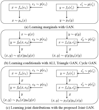
It is desirable to build a generative-model learning framework from which one may sample from a fully-learned joint distribution. We design a new GAN framework that learns the joint distribution by decomposing it into the product of a marginal and a conditional distribution(s), each learned via adversarial training (see Figure 1(c) for illustration). The resulting model may then be employed in several distinct applications: () synthesis of draws from any of the marginals; () synthesis of draws from the conditionals when other random variables are observed, i.e., imputation; () or we may simultaneously draw all random variables from the joint distribution.
For the special case of two random variables, the proposed model consists of four generators and a softmax critic function. The design includes two generators for the marginals, two for the conditionals, and a single 5-way critic (discriminator) trained to distinguish pairs of real data from four different kinds of synthetic data. These five modules are implemented as neural networks, which share parameters for efficiency and are optimized jointly via adversarial learning. We also consider an example with three random variables.
The contributions of this work are summarized as follows. () We present the first GAN-enabled framework that allows for full joint-distribution learning of multiple random variables. Unlike existing models, the proposed framework learns marginals and conditionals simultaneously. () We share parameters of the generator models, and thus the resulting model does not have a significant increase in the number of parameters relative to prior work that only considered conditionals (ALI, Triangle GAN, CycleGAN, etc.) or marginals (traditional GAN). () Unlike existing approaches, we consolidate all real vs. artificial sample comparisons into a single softmax-based critic function. () While the main focus is on the case of two random variables, we extend the proposed model to learning the joint distribution of three or more random variables. () We apply the proposed model for both unsupervised and supervised learning paradigms.
2 Background
To simplify the presentation, we first consider joint modeling of two random variables, with the setup generalized in Sec. 3.2 to the case of more than two domains. For the two-random-variable case, consider marginal distributions and defined over two random variables and , respectively. Typically, we have samples but not an explicit density form for and , i.e., ensembles and are available for learning. In general, their joint distribution can be written as the product of a marginal and a conditional in two ways: . One random variable can be synthesized (or inferred) given the other using conditional distributions, and .
2.1 Generative Adversarial Networks
Nonparametric sampling from marginal distributions and can be accomplished via adversarial learning (Goodfellow et al., 2014), which provides a sampling mechanism that only requires gradient backpropagation, avoiding the need to explicitly adopt a form for the marginals. Specifically, instead of sampling directly from an (assumed) parametric distribution for the desired marginal, the target random variable is generated as a deterministic transformation of an easy-to-sample, independent noise source, e.g., Gaussian distribution. The sampling procedure for the marginals, implicitly defined as and , is carried out through the following two generative processes:
| (1) | ||||
| (2) |
where and are two marginal generators, specified as neural networks with parameters and , respectively. and are assumed to be simple distributions, , isotropic Gaussian. The generative processes manifested by (1) and (2) are illustrated in Figure 1(a). Within the models, stochasticity in and is manifested via draws from and , and respective neural networks and transform draws from these simple distributions such that they are approximately consistent with draws from and .
For this purpose, GAN trains a -parameterized critic function , to distinguish samples generated from and . Formally, the minimax objective of GAN is
| (3) | ||||
with expectations and approximated via sampling, and is the sigmoid function. As shown in Goodfellow et al. (2014), the equilibrium of the objective in (3) is achieved if and only if .
Similarly, we can design a corresponding minimax objective that is similar to (3) to match the marginal to .
2.2 Adversarially Learned Inference
In the same spirit, sampling from conditional distributions and can be also achieved as a deterministic transformation of two inputs, the variable in the source domain as a covariate, plus an independent source of noise. Specifically, the sampling procedure for the conditionals and is modeled as
| (4) | ||||
| (5) |
where and are two conditional generators, specified as neural networks with parameters and , respectively. In practice, the inputs of and are concatenated. As in GAN, and are two simple distributions that provide the stochasticity when generating given , and vice versa. The conditional generative processes manifested in (4) and (5) are illustrated in Figure 1(b),
ALI (Dumoulin et al., 2017) learns the two desired conditionals by matching joint distributions and , using a critic function similar to (3). The minimax objective of ALI can be written as
| (6) | ||||
The equilibrium of the objective in (6) is achieved if and only if .
While ALI is able to match joint distributions using (6), only conditional distributions and are learned, thus assuming access to (samples from) the true marginal distributions and , respectively.
3 Adversarial Joint Distribution Learning
Below we discuss fully learning the joint distribution of two random variables in both supervised and unsupervised settings. By “supervised” it is meant that we have access to joint empirical data , and by “unsupervised” it is meant that we have access to empirical draws of and , but not paired observations from the joint distribution.
3.1 JointGAN
Since , a simple way to achieve joint-distribution learning is to first learn models for the two marginals separately, using a pair of traditional GANs, followed by training an independent ALI model for the two conditionals. However, such a two-step training procedure is suboptimal, as there is no information flow between marginals and conditionals during training. This suboptimality is demonstrated in the experiments. Additionally, a two-step learning process becomes cumbersome when considering more than two random variables.
Alternatively, we consider learning to sample from conditionals via and , while also learning to sample from marginals via and . All model training is performed simultaneously. We term our model JointGAN for full GAN analysis of joint random variables.
Access to Paired Empirical Draws
In this setting, we assume access to samples from the true (empirical) joint distribution . The models we seek to learn constitute two means of approximating draws from the true distribution , i.e., and , as shown in Figure 1(c):
| (7) | ||||
| (8) |
where , , and are neural networks as defined previously. , , and are independent noise. Note that the only difference between and is that the function has another conditional input when compared with . Therefore, in implementation, we couple the parameters and together. Similarly, and are also coupled together. Specifically, and are implemented as
| (9) |
where is an all-zero tensor which has the same size as or . As a result, (7) and (8) have almost the same number of parameters as ALI-like approaches.
The following notation is introduced for simplicity of illustration:
| (10) | ||||||
where , , and are implicitly defined in (4), (5), (7) and (8). Note that is simply the empirical joint distribution.
When learning, we wish to impose that the five distributions in (10) should be identical. Toward this end, an adversarial objective is specified. Joint pairs are drawn from the five distributions in (10), and a critic function is learned to discriminate among them, while the four generators are trained to mislead the critic. Naively, for JointGAN, one can use 4 binary critics to mimic a 5-class classifier. Departing from previous work such as Gan et al. (2017a), here the discriminator is implemented directly as a 5-way softmax classifier. Compared with using multiple binary classifiers, this design is more principled in that we avoid multiple critics resulting in possibly conflicting (real vs. synthetic) assessments.
Let the critic (in the 4-simplex) be a -parameterized neural network with softmax on the top layer, i.e., and , where is an entry of . The minimax objective for JointGAN, , is given by
| (11) | |||
The above objective (11) has taken into consideration the model design that and are coupled together, with the same for and ; thus and are not present in (11). Note that expectation is approximated using empirical joint samples, expectations and are both approximated with purely synthesized joint samples, while and are approximated using conditionally synthesized samples, given samples from the empirical marginals. The following proposition characterizes the solution of (11) in terms of the joint distributions.
Proposition 1
The equilibrium for the minimax objective in (11) is achieved if and only if .
The proof is provided in Appendix A.
No Access to Paired Empirical Draws
3.2 Extension to multiple domains
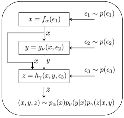
The above formulation may be extended to the case of three or more joint random variables. However, for random variables, there are different ways in which the joint distribution can be factorized. For example, for joint random variables , there are possibly six different forms of the model. One must have access to all the six instantiations of these models, if the goal is to be able to generate (impute) samples from all conditionals. However, not all modeled forms of need to be considered, if there is not interest in the corresponding form of the conditional. Below, we consider two specific forms of the model:
| (13) | ||||
| (14) |
Typically, the joint draws from may not be easy to access; therefore, we assume that only empirical draws from and are available. For the purpose of adversarial learning, we let the critic be a 6-class softmax classifier that aims to distinguish samples from the following 6 distributions:
After training, one may synthesize , impute from observed , or impute from , etc. Examples of this learning paradigm is demonstrated in the experiments. Interestingly, when implementing a sampling-based method for the above models, skip connections are manifested naturally as a result of the partitioning of the joint distribution, e.g., via and . This is illustrated in Figure 2, for .
4 Related work
Adversarial methods for joint distribution learning can be roughly divided into two categories, depending on the application: () generation and inference if one of the domains consists of (stochastic) latent variables, and () conditional data synthesis if both domains consists of observed pairs of random variables. Below, we review related work from these two perspectives.
Generation and inference
The joint distribution of data and latent variables or codes can be considered in two (symmetric) forms: () from observed data samples fed through the encoder to yield codes, i.e., inference, and () from codes drawn from a simple prior and propagated through the decoder to manifest data samples, i.e., generation. ALI (Dumoulin et al., 2017) and BiGAN (Donahue et al., 2017) proposed fully adversarial methods for this purpose. There are also many recent works concerned with integrating variational autoencoder (VAE) (Kingma & Welling, 2013; Pu et al., 2016) and GAN concepts for improved data generation and latent code inference (Hu et al., 2017). Representative work includes the AAE (Makhzani et al., 2015), VAE-GAN (Larsen et al., 2015), AVB (Mescheder et al., 2017), AS-VAE (Pu et al., 2017), SVAE (Chen et al., 2018), etc.
Conditional data synthesis
Conditional GAN can be readily used for conditional-data synthesis if paired data are available. Multiple conditional GANs have been proposed to generate the images based on class labels (Mirza & Osindero, 2014), attributes (Perarnau et al., 2016), text (Reed et al., 2016; Xu et al., 2017) and other images (Isola et al., 2017). Often, only the mapping from one direction (a single conditional) is learned. Triangle GAN (Gan et al., 2017a) and Triple GAN (Li et al., 2017b) can be used to learn bi-directional mappings (both conditionals) in a semi-supervised learning setup. Unsupervised learning methods were also developed for this task. CycleGAN (Zhu et al., 2017) proposed to use two generators to model the conditionals and two critics to decide whether a generated sample is synthesized, in each individual domain. Further, additional reconstruction losses were introduced to impose cycle consistency. Similar work includes DiscoGAN (Kim et al., 2017), DualGAN (Yi et al., 2017) and UNIT (Liu et al., 2017).
CoGAN (Liu & Tuzel, 2016) can be used to achieve joint distribution learning. However, the joint distribution is only roughly approximated by the marginals, via sharing low-layer weights of the generators, hence not learning the true (empirical) joint distributions in a principled way.
All the other previously proposed models focus on learning to sample from the conditionals given samples from one of the true (empirical) marginals, while the proposed model, to the best of the authors’ knowledge, is the first attempt to learn a full joint distribution of two or more observed random variables. Moreover, this paper presents the first consolidation of multiple binary critics into a single unified softmax-based critic.
We observe that the proposed model, JointGAN, may follow naturally in concept from GAN (Goodfellow et al., 2014) and ALI (Donahue et al., 2017; Dumoulin et al., 2017). However, there are several keys to obtaining good performance. Specifically, () the condition distribution setup naturally yields skip connections in the architecture. () Compared with using multiple binary critics, the softmax-based critic can be considered as sharing the parameters among all the binary critics except the top layer. This also imposes the critic embedding the generated samples from different ways into a common latent space and reduces the number of parameters. () The weight-sharing constraint among generators enforces that synthesized images from the marginal and conditional generator share a common latent space, and also further reduces the number of parameters in the network.
5 Experiments
Adam (Kingma & Ba, 2014) with learning rate 0.0002 is utilized for optimization of the JointGAN objectives. All noise vectors , , and are drawn from a distribution, with the dimension of each set to 100. Besides the results presented in this section, more results can be found in Appendix C.2. The code can be found at https://github.com/sdai654416/Joint-GAN.
5.1 Joint modeling multi-domain images
Datasets
We present results on five datasets: edges shoes (Yu & Grauman, 2014), edgeshandbags (Zhu et al., 2016), Google mapsaerial photos (Isola et al., 2017), labelsfacades (Tyleček & Šára, 2013) and labels cityscapes (Cordts et al., 2016). All of these datasets are two-domain image pairs.
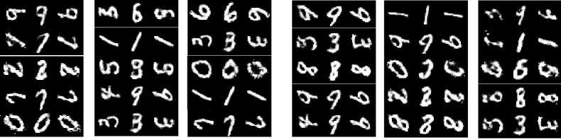
For three-domain images, we create a new dataset by combining labelsfacades pairs and labelscityscapes pairs into facadeslabelscityscapes tuples. In this dataset, only empirical draws from and are available. Another new dataset is created based on MNIST, where the three image domains are the MNIST images, clockwise transposed ones, and anticlockwise transposed ones.
Baseline
As described in Sec. 3.1, a two-step model is implemented as the baseline. Specifically, WGAN-GP (Gulrajani et al., 2017) is employed to model the two marginals; Pix2pix (Isola et al., 2017) and CycleGAN (Zhu et al., 2017) are utilized to model the conditionals for the case with and without access to paired empirical draws, respectively.
Network Architectures
For generators, we employed the U-net (Ronneberger et al., 2015) which has been demonstrated to achieve impressive results for image-to-image translation. Following Isola et al. (2017), PatchGAN is employed for the discriminator, which provides real vs. synthesized prediction on overlapping image patches.
5.1.1 Qualitative Results
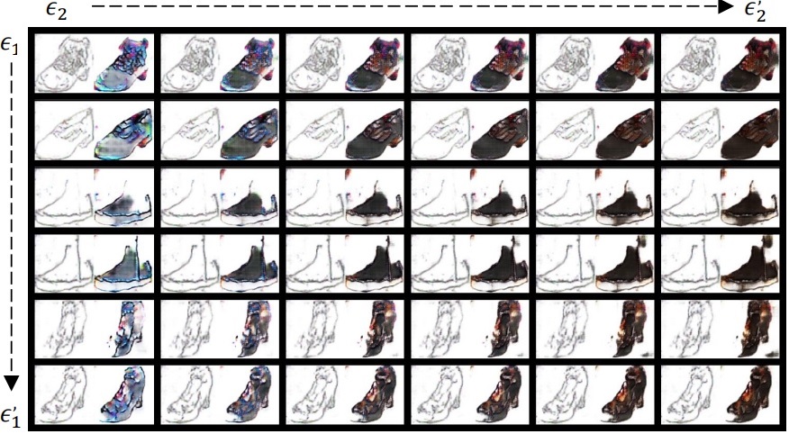
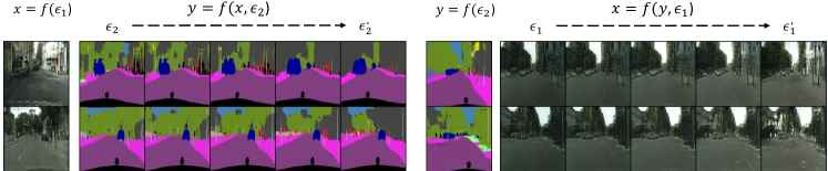
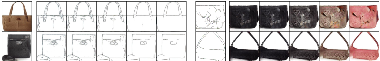
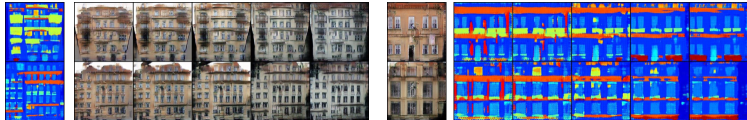
Figures 3 and 4 show the results trained on paired data. All the image pairs are generated from random noise. For Figure 4, we first draw and to generate the top-left image pairs and bottom-right image pairs according to (7). All remaining image pairs are generated from the noise pair made by linear interpolation between and , and between and , respectively, also via (7). For Figure 3, in each row of the left block, the column is first generated from , and then the images of the right part are generated based on the leftmost image and an additional noise vector linear-interpolated between two random points and . The images in the right block are produced in a similar way.
These results demonstrate that our model is able to generate both realistic and highly coherent image pairs. In addition, the interpolation experiments illustrate that our model maintains smooth transitions in the latent space, with each point in the latent space corresponding to a plausible image. For example, in the edgeshandbags dataset, it can be seen that the edges smoothly transforming from complicated structures into simple ones, and the color of the handbags transforming from black to red. The quality of images generated from the baseline is much worse than ours, and are provided in Appendix C.1.
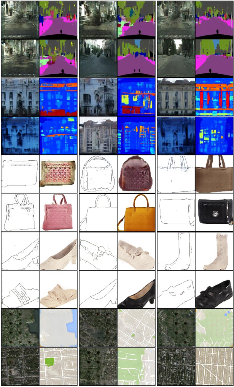
Figure 5 shows the generated samples trained on unpaired data. Our model is able to produce image pairs whose quality are close to the samples trained on paired data.
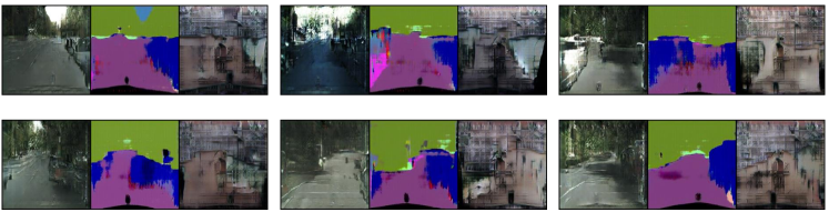
Figures 6 and 7 show the generated samples from models trained on three-domain images. The generated images in each tuple are highly correlated. Interestingly, in Figure 7, the synthesized labels strive to be consistent with both the generated street scene and facade photos.
| Method | Realism | Relevance |
|---|---|---|
| Trained with paired data | ||
| WGAN-GP + Pix2pix wins | 2.32% | 3.1% |
| JointGAN wins | 17.93% | 36.32% |
| Not distinguishable | 79.75% | 60.58% |
| Trained with unpaired data | ||
| WGAN-GP + CycleGAN wins | 0.13% | 1.31% |
| JointGAN wins | 81.55% | 40.87% |
| Not distinguishable | 18.32% | 57.82% |
5.1.2 Quantitative Results
We perform a detailed quantitative analysis on the two-domain image-pair task.
Human Evaluation
We perform human evaluation using Amazon Mechanical Turk (AMT), and present human evaluation results on the relevance and realism of generated pairs in both the cases with or without access to paired empirical samples. In each survey, we compare JointGAN and the two-step baseline by taking a random sample of 100 generated image pairs (5 datasets, 20 samples on each dataset), and ask the human evaluator to select which sample is more realistic and the content of which pairs are more relevant. We obtained roughly 44 responses per data sample (4378 samples in total) and the results are shown in Table 1. Clearly, human analysis suggest that our JointGAN produces higher-quality samples when compared with the two-step baseline, verifying the effectiveness of learning the marginal and conditional simultaneously.
Relevance Score
| edgesshoes | edgeshandbags | labelscityscapes | labelsfacades | mapssatellites | |
|---|---|---|---|---|---|
| True pairs | 0.684 | 0.672 | 0.591 | 0.529 | 0.514 |
| Random pairs | 0.008 | 0.005 | 0.012 | 0.011 | 0.054 |
| Other pairs | 0.113 | 0.139 | 0.092 | 0.076 | 0.081 |
| WGAN-GP + Pix2pix | 0.352 | 0.343 | 0.301 | 0.288 | 0.125 |
| JointGAN (paired) | 0.488 | 0.489 | 0.377 | 0.364 | 0.328 |
| WGAN-GP + CycleGAN | 0.203 | 0.195 | 0.201 | 0.139 | 0.091 |
| JointGAN (unpaired) | 0.452 | 0.461 | 0.339 | 0.341 | 0.299 |
We use relevance score to evaluate the quality and relevance of two generated images. The relevance score is calculated as the cosine similarity between two images that are embedded into a shared latent space, which are learned via training a ranking model (Huang et al., 2013). Details are provided in Appendix B. The final relevance score is the average over all the individual relevance scores on each pair. Results are summarized in Table 2. Our JointGAN provides significantly better results than the two-step baselines, especially when we do not have access to the paired empirical samples.
Besides the results of our model and baselines, we also present results on three types of real images: () True pairs: this is the real image pairs from the same dataset but not used for training the ranking model; () Random pairs: the images are from the same dataset but the content of two images are not correlated; () Other pairs: the images are correlated but sampled from a dataset different from the training set. We can see in Table 2 that the first one obtains a high relevance score while the latter two have a very low score, which shows that the relevance score metric assigns a low value when either the content of generated image pairs is not correlated or the images are not plausibly like the training set. It demonstrates that this metric correlates well with the quality of generated image pairs.
5.2 Joint modeling caption features and images
Setup
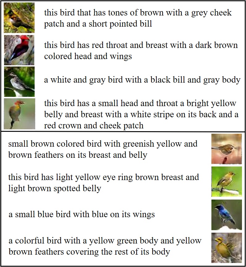
Our model is next evaluated on the Caltech-UCSD Birds dataset (Welinder et al., 2010), in which each image of bird is paired with 10 different captions. Since generating realistic text using GAN itself is a challenging task, in this work, we train our model on pairs of caption features and images. The caption features are obtained from a pretrained word-level CNN-LSTM autoencoder (Gan et al., 2017b), which aims to achieve a one-to-one mapping between the captions and the features. We then train JointGAN based on the caption features and their corresponding images (the paired data for training JointGAN use CNN-generated text features, which avoids issues of training GAN for text generation). Finally to visualize the results, we use the pretrained LSTM decoder to decode the generated features back to captions. We employ StackGAN-stage-I (Zhang et al., 2017a) for generating images from caption features while a CNN is utilized to generate caption features from images. Details are provided in Appendix D.
Qualitative Results
Figure 8 shows the qualitative results of JointGAN: () generate images from noise and then conditionally generate caption features, and () generate caption features from noise and then conditionally generate images. The results show high-quality and diverse image generation, and strong coherent relationship between each pair of the caption feature and image. It demonstrates the robustness of our model, in that it not only generates realistic multi-domain images but also handles well different datasets such as caption feature and image pairs.
6 Conclusion
We propose JointGAN, a new framework for multi-domain joint distribution learning. The joint distribution is learned via decomposing it into the product of a marginal and a conditional distribution(s), each learned via adversarial training. JointGAN allows interesting applications since it provides freedom to draw samples from various marginalized or conditional distributions. We consider joint analysis of two and three domains, and demonstrate that JointGAN achieves significantly better results than a two-step baseline model, both qualitatively and quantitatively.
Acknowledgements
This research was supported in part by DARPA, DOE, NIH, ONR and NSF.
References
- Chen et al. (2018) Chen, L., Dai, S., Pu, Y., Zhou, E., Li, C., Su, Q., Chen, C., and Carin, L. Symmetric variational autoencoder and connections to adversarial learning. In AISTATS, 2018.
- Cordts et al. (2016) Cordts, M., Omran, M., Ramos, S., Rehfeld, T., Enzweiler, M., Benenson, R., Franke, U., Roth, S., and Schiele, B. The cityscapes dataset for semantic urban scene understanding. In CVPR, 2016.
- Donahue et al. (2017) Donahue, J., Krähenbühl, P., and Darrell, T. Adversarial feature learning. In ICLR, 2017.
- Dumoulin et al. (2017) Dumoulin, V., Belghazi, I., Poole, B., Mastropietro, O., Lamb, A., Arjovsky, M., and Courville, A. Adversarially learned inference. In ICLR, 2017.
- Gan et al. (2017a) Gan, Z., Chen, L., Wang, W., Pu, Y., Zhang, Y., Liu, H., Li, C., and Carin, L. Triangle generative adversarial networks. In NIPS, 2017a.
- Gan et al. (2017b) Gan, Z., Pu, Y., Henao, R., Li, C., He, X., and Carin, L. Learning generic sentence representations using convolutional neural networks. In EMNLP, 2017b.
- Goodfellow et al. (2014) Goodfellow, I., Pouget-Abadie, J., Mirza, M., Xu, B., Warde-Farley, D., Ozair, S., Courville, A., and Bengio, Y. Generative adversarial nets. In NIPS, 2014.
- Gulrajani et al. (2017) Gulrajani, I., Ahmed, F., Arjovsky, M., Dumoulin, V., and Courville, A. C. Improved training of Wasserstein GANs. In NIPS, 2017.
- Hu et al. (2017) Hu, Z., Yang, Z., Salakhutdinov, R., and Xing, E. P. On unifying deep generative models. arXiv preprint arXiv:1706.00550, 2017.
- Huang et al. (2013) Huang, P.-S., He, X., Gao, J., Deng, L., Acero, A., and Heck, L. Learning deep structured semantic models for web search using clickthrough data. In CIKM, 2013.
- Isola et al. (2017) Isola, P., Zhu, J.-Y., Zhou, T., and Efros, A. A. Image-to-image translation with conditional adversarial networks. In CVPR, 2017.
- Kim et al. (2017) Kim, T., Cha, M., Kim, H., Lee, J., and Kim, J. Learning to discover cross-domain relations with generative adversarial networks. In ICML, 2017.
- Kingma & Ba (2014) Kingma, D. P. and Ba, J. Adam: A method for stochastic optimization. arXiv preprint arXiv:1412.6980, 2014.
- Kingma & Welling (2013) Kingma, D. P. and Welling, M. Auto-encoding variational bayes. arXiv preprint arXiv:1312.6114, 2013.
- Larsen et al. (2015) Larsen, A. B. L., Sønderby, S. K., Larochelle, H., and Winther, O. Autoencoding beyond pixels using a learned similarity metric. arXiv preprint arXiv:1512.09300, 2015.
- Li et al. (2017a) Li, C., Liu, H., Chen, C., Pu, Y., Chen, L., Henao, R., and Carin, L. Alice: Towards understanding adversarial learning for joint distribution matching. In NIPS, 2017a.
- Li et al. (2017b) Li, C., Xu, K., Zhu, J., and Zhang, B. Triple generative adversarial nets. In NIPS, 2017b.
- Liu & Tuzel (2016) Liu, M.-Y. and Tuzel, O. Coupled generative adversarial networks. In NIPS, 2016.
- Liu et al. (2017) Liu, M.-Y., Breuel, T., and Kautz, J. Unsupervised image-to-image translation networks. In NIPS, 2017.
- Makhzani et al. (2015) Makhzani, A., Shlens, J., Jaitly, N., Goodfellow, I., and Frey, B. Adversarial autoencoders. arXiv preprint arXiv:1511.05644, 2015.
- Mescheder et al. (2017) Mescheder, L., Nowozin, S., and Geiger, A. Adversarial variational bayes: Unifying variational autoencoders and generative adversarial networks. In ICML, 2017.
- Mirza & Osindero (2014) Mirza, M. and Osindero, S. Conditional generative adversarial nets. In arXiv preprint arXiv:1411.1784, 2014.
- Perarnau et al. (2016) Perarnau, G., van de Weijer, J., Raducanu, B., and Álvarez, J. M. Invertible conditional gans for image editing. arXiv preprint arXiv:1611.06355, 2016.
- Pu et al. (2016) Pu, Y., Gan, Z., Henao, R., Yuan, X., Li, C., Stevens, A., and Carin, L. Variational autoencoder for deep learning of images, labels and captions. In NIPS, 2016.
- Pu et al. (2017) Pu, Y., Wang, W., Henao, R., Chen, L., Gan, Z., Li, C., and Carin, L. Adversarial symmetric variational autoencoder. In NIPS, 2017.
- Radford et al. (2016) Radford, A., Metz, L., and Chintala, S. Unsupervised representation learning with deep convolutional generative adversarial networks. ICLR, 2016.
- Reed et al. (2016) Reed, S., Akata, Z., Yan, X., Logeswaran, L., Schiele, B., and Lee, H. Generative adversarial text to image synthesis. In ICML, 2016.
- Ronneberger et al. (2015) Ronneberger, O., Fischer, P., and Brox, T. U-net: Convolutional networks for biomedical image segmentation. In MICCAI, 2015.
- Tao et al. (2018) Tao, C., Chen, L., Henao, R., Feng, J., and Carin, L. Chi-square generative adversarial network. In ICML, 2018.
- Tyleček & Šára (2013) Tyleček, R. and Šára, R. Spatial pattern templates for recognition of objects with regular structure. In GCPR, 2013.
- Welinder et al. (2010) Welinder, P., Branson, S., Mita, T., Wah, C., Schroff, F., Belongie, S., and Perona, P. Caltech-UCSD Birds 200. Technical report, California Institute of Technology, 2010.
- Xu et al. (2017) Xu, T., Zhang, P., Huang, Q., Zhang, H., Gan, Z., Huang, X., and He, X. Attngan: Fine-grained text to image generation with attentional generative adversarial networks. arXiv preprint arXiv:1711.10485, 2017.
- Yi et al. (2017) Yi, Z., Zhang, H., Tan, P., and Gong, M. Dualgan: Unsupervised dual learning for image-to-image translation. In CVPR, 2017.
- Yu & Grauman (2014) Yu, A. and Grauman, K. Fine-grained visual comparisons with local learning. In CVPR, 2014.
- Yu et al. (2017) Yu, L., Zhang, W., Wang, J., and Yu, Y. Seqgan: Sequence generative adversarial nets with policy gradient. In AAAI, 2017.
- Zhang et al. (2017a) Zhang, H., Xu, T., Li, H., Zhang, S., and Metaxas, D. Stackgan: Text to photo-realistic image synthesis with stacked generative adversarial networks. In ICCV, 2017a.
- Zhang et al. (2017b) Zhang, Y., Gan, Z., Fan, K., Chen, Z., Henao, R., Shen, D., and Carin, L. Adversarial feature matching for text generation. In ICML, 2017b.
- Zhu et al. (2016) Zhu, J.-Y., Krähenbühl, P., Shechtman, E., and Efros, A. A. Generative visual manipulation on the natural image manifold. In ECCV, 2016.
- Zhu et al. (2017) Zhu, J.-Y., Park, T., Isola, P., and Efros, A. A. Unpaired image-to-image translation using cycle-consistent adversarial networks. In CVPR, 2017.