Proposal for the creation and observation of a ghost trilobite chemical bond

Abstract

The “trilobite” type of molecule, predicted in 2000 and observed experimentally in 2015, arises when a Rydberg electron exerts a weak attractive force on a neutral ground state atom. Such molecules have bond lengths exceeding 100 nm. The ultra-long-range chemical bond between the two atoms is a nonperturbative linear combination of the many degenerate electronic states associated with high principal quantum numbers, and the resulting electron probability distribution closely resembles a fossil trilobite from antiquity. We show how to coherently engineer this same long-range orbital through a sequence of electric and magnetic field pulses even when the ground state atom is not present, and propose several methods to observe the resulting orbital. The existence of such a ghost chemical bond in which an electron reaches out from one atom to a nonexistent second atom is a consequence of the high level degeneracy.

Many stunning experiments in recent years have demonstrated that a novel type of chemical binding occurs between a highly excited Rydberg atom and a neutral ground-state atom Bendkowsky et al. (2009); Booth et al. (2015); Niederprüm et al. (2016). The Fermi pseudopotential reveals that this weak bonding derives from the low-energy scattering of the Rydberg electron off the neutral atom, and furthermore describes this interaction with a delta function proportional to the $s$-wave electron-atom scattering length $a_{s}$ Fermi (1934); Greene et al. (2000). Rydberg molecules have been observed in Cs, Rb, and Sr, all of which have $a_{s}<0$ Bendkowsky et al. (2009); Tallant et al. (2012); DeSalvo et al. (2015). The most interesting Rydberg molecules are the highly polar varieties, dubbed “trilobites” and “butterflies” for the unusual appearance of their electronic densities Hamilton et al. (2002); Chibisov et al. (2002). In these molecules degenerate non-penetrating high angular momentum $l$ states hybridize to maximize either the electron’s probability (trilobite) or probability gradient (butterfly) near the ground state atom Booth et al. (2015); Niederprüm et al. (2016); Kleinbach et al. (2017).

The electronic wave function of one of these molecules having a bond length $R_{b}$ is

$$\Psi(R_{b},\vec{r})=\mathcal{N}\sum_{l=l_{0}}^{n-1}c_{nl,x}^{b}\phi_{nl}(\vec{r}),$$ (1)

where $\mathcal{N}$ is a normalization constant, $l_{0}$ restricts the summation to degenerate states ($l_{0}\approx 3$ in alkali atoms) and $\phi_{nl}(\vec{r})=\frac{u_{nl}(r)}{r}Y_{l0}(\theta,\phi)$ are standard hydrogenic Rydberg wave functions. The label $x$ refers to the type of molecule (i.e. trilobite or butterfly). Due to cylindrical symmetry and the functional form of the pseudopotential, $m_{l}=0$. The coefficients $c_{nl,x}^{b}$ are determined by diagonalizing the Fermi pseudopotential in the basis of degenerate hydrogenic states. For example, $c_{nl,\text{trilobite}}^{b}=\phi_{nl}(\vec{R}_{b})$. For a general target state these coefficients can be compactly expressed as a vector, $\vec{c}_{T}$.

The degeneracy needed to form these exotic states is exact for all $l$ in nonrelativistic hydrogen. Since the hydrogen-electron scattering lengths are both positive, the repulsive trilobite potential curves cannot support vibrational bound states. Nevertheless, theoretical evidence suggests that the Rydberg electron-atom interaction still evinces resonant behavior related to the stationary points of the potential curves Pérez-Ríos et al. (2016); Tarana and Čurík (2016). These are located at $R_{b}$ satisfying $u_{n0}(R_{b})=0$ Chibisov et al. (2000). The index $b$ thus labels a series of trilobite states with specific bond lengths and nodal structure; furthermore, at these $R_{b}$ the wave function is dominated by just a few eigenfunctions of the Schrödinger equation in elliptical coordinates Granger et al. (2001). Like trilobite molecules, butterfly molecules are bound by electron-atom scattering, although they additionally depend on a $p$-wave shape resonance in the electron-atom scattering and the form of the $p$-wave pseudopotential involves gradient operators acting on the wave function Hamilton et al. (2002); Chibisov et al. (2002); Niederprüm et al. (2016).

This letter shows that it is possible to create these chemical bonding orbitals with the ground state atom absent, and for this reason we refer to the electronic wave function (equation 1) as a ghost chemical bond. By employing a carefully engineered sequence of alternating magnetic and electric fields, we evolve the wave function from an isotropic $ns$ state into precisely the same orbital that would form a chemical bond if a ground state atom were located at $R_{b}$. The time evolution is described via unitary operators in degenerate first-order perturbation theory. A gradient ascent algorithm derived from optimal control theory optimizes the field sequence to ensure excellent overlap with the target state. Two detection mechanisms are proposed to image and study this chemical bond, either in the “ghost” or in the true trilobite molecule. Atomic units are used throughout.

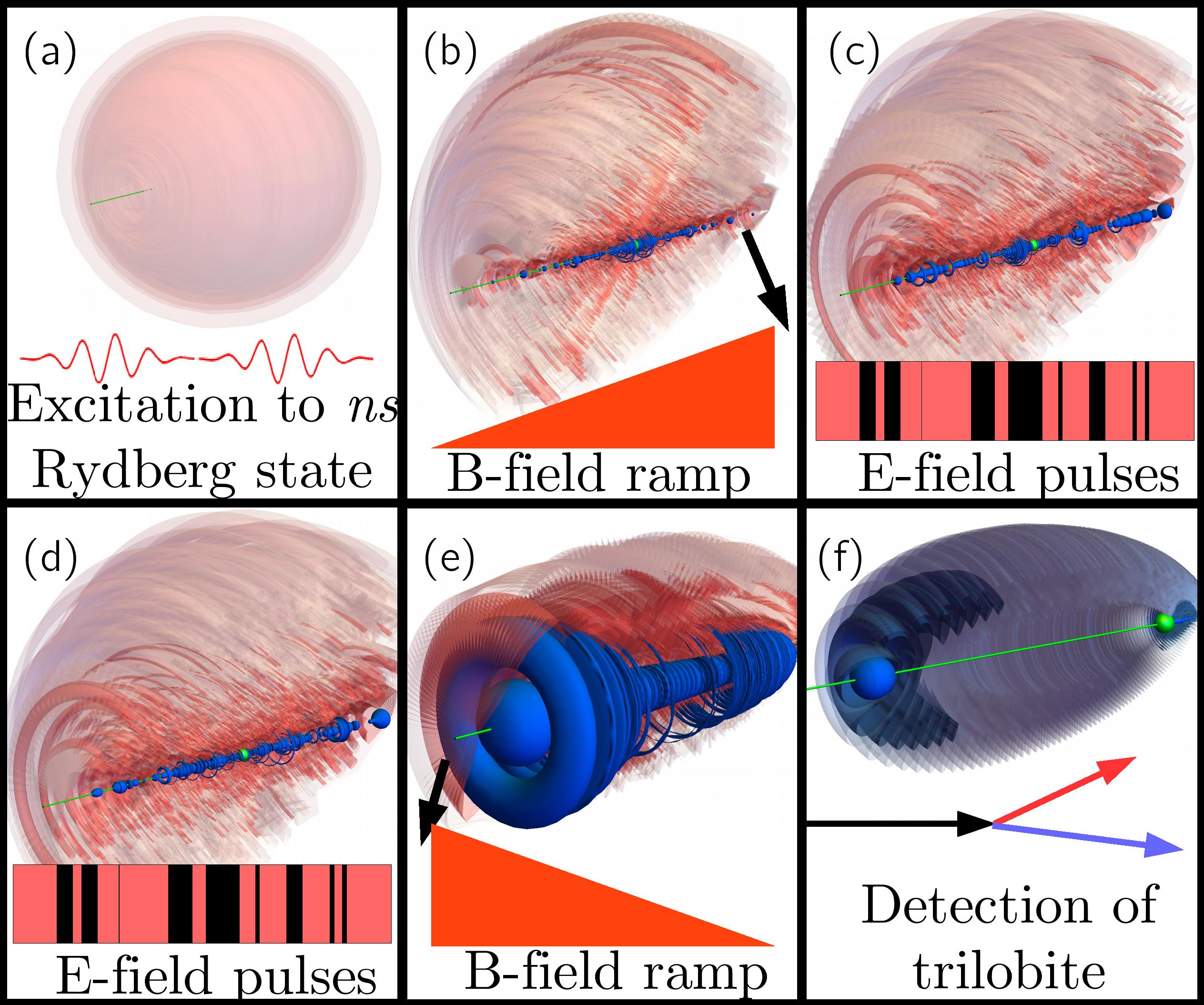
Figure 1: The proposed scheme, illustrated using the $n=70,b=1$ trilobite as an example. The electronic probability is displayed in each panel usng three isosurfaces, defined where $|\Psi(x,y,z)|^{2}$ is $C$% of $\text{Max}\left(|\Psi_{\text{trilobite}}(R_{b=1};x,y,z)|^{2}\right)$. They are cut away to reveal the inner structure. The Rydberg ion, not to scale, is the green sphere and the green line, parallel to the $z$ axis, provides a scale and is 1.1$\times 10^{4}a_{0}$ long. The color scheme for panels a-e is: bright blue when $C=1.54$, red when $C=0.154$, and translucent pink when $C=1.54\times 10^{-2}$. For panel f: bright blue for $C=15.4$, darker blue when $C=1.54$, and transparent blue when $C=0.308$. a) First, an $ns$ Rydberg state is created. b) Next, the magnetic field ramps on, creating a quadratic Zeeman state. c,d) After the magnetic field reaches its maximum value, many short electric field pulses are applied in addition to the magnetic field, creating complicated superpositions of the degenerate states. At different points in the sequence the wave function is strongly mixed. e) At the end of the sequence of electric field pulses, a proto-trilobite is created. The magnetic field ramps off and this state evolves into the trilobite state, f), which is detected.

Fig. 1 depicts the proposed experimental implementation of this concept. First, a hydrogen atom is excited to an $ns$ Rydberg state. Next, a magnetic field ramps on to a final amplitude $B$. Immediately after the ramp, a sequence of $N$ electric field pulses of amplitude $F$ are applied. After the $N^{\text{th}}$ pulse the magnetic field ramps off. For the $n=70$ Rydberg state considered here, the ramp times are typically tens of $\mu$s, while the electric field durations and separations are several nanoseconds each, lasting in total several tens of $\mu$s as well. This whole process thus occurs within the natural radiative and blackbody lifetime of the Rydberg state. The trilobite state is particularly long-lived since it is an admixture of predominantly high$-l$ states and its decay rate is therefore mostly affected by blackbody radiation. We set a conservative lower lifetime bound at 200$\mu$s. This time increases with decreasing ambient temperature, extending to several milliseconds at 10K Farley and Wing (1981); Gallagher and Cooke (1979); Zhou and Spruch (1994); Gallagher (2005); Beterov et al. (2009). As lower $l$ states bleed away, the dominant components of the trilobite state persist, leading to the remarkable scenario where the Rydberg electron remains localized in a small point several hundreds of nanometers away from the proton for many tens of microseconds. Dephasing caused by the small, MHz-scale energy splittings between fine structure levels of the low-$l$ states is limited since these components decay sooner, and additionally this dephasing is further eliminated since the final state is predominately high-$l$ states. These small energy splittings could impact the fidelity as these low-$l$ states are more prominent during the time evolution, but the presence of the large static magnetic field will prevent dephasing between different fine structure states due to the Paschen-Back effect Note (1). Interesting effects arise if a small electric field is pulsed on in this final state. The ghost chemical bond will revive every $\tau=\frac{2\pi}{3Fn}$, which is about 37 ns for a $0.1$V/cm electric field. Furthermore, the decay mode of the ghost molecule will change as the trilobite state is a linear combination of non-degenerate Stark eigenstates. Details describing the physical considerations guiding this scheme design and some of the relevant parameters are found in the supplementary material Note (1).

Fig. 2 displays several ghost chemical bonds which can be created by this scheme. Perhaps the most distinctive characteristic of trilobite bonds is their nodal structure: as $b$ increments by one, a new lobe in the direction perpendicular to the intermolecular axis appears (Fig.2a shows a $b=3$ trilobite). Moreover, they are remarkably localized, maximally so in the $b=1$ trilobite shown in Fig. 1f, where 20% of the electron density occupies a region around the ghost atom smaller than 0.1% of the total classically allowed volume. This localization is because the trilobite state, by construction, is the representation of the three-dimensional delta function in the finite basis of hydrogenic states in a single $n$-manifold. The butterfly molecule chemical bond (Fig. 2b) has a bond length an order of magnitude smaller than the trilobite, and the wave function, fanning out into a winglike structure, fills much more of the classically allowed volume. Rydberg molecules need not be exclusively diatomic: polyatomic Rydberg trilobite or butterfly molecules with more than one ground state atom lying within the Rydberg wave function have been studied theoretically Liu and Rost (2006); Eiles et al. (2016) but are challenging to observe in an experiment due to the low probability of finding the right configuration of three atoms. This restriction is of course lifted for bonds to nonexistent ghost atoms (Fig. 2c) The coefficients $c_{nl,x}^{b}$ for these other Rydberg chemical bonds are provided in the supplementary material Note (1), and it should be remembered that the proposed method is generic to any set of coefficients since the key requirement is that only the degenerate $n$-manifold is included. Time-dependent wave packets or the exotic giant dipole states, hydrogen atoms exposed to crossed fields such that the electron localizes in an anisotropic harmonic oscillator potential extremely far from the nucleus, are not allowed in this scheme as they are superpositions of non-degenerate states Averbukh et al. (1999). The Stark state (Fig. 2d) and the Zeeman state (Fig. 1b) highlight that even localized electron wave functions in static fields are entirely different from Rydberg molecule wave functions.

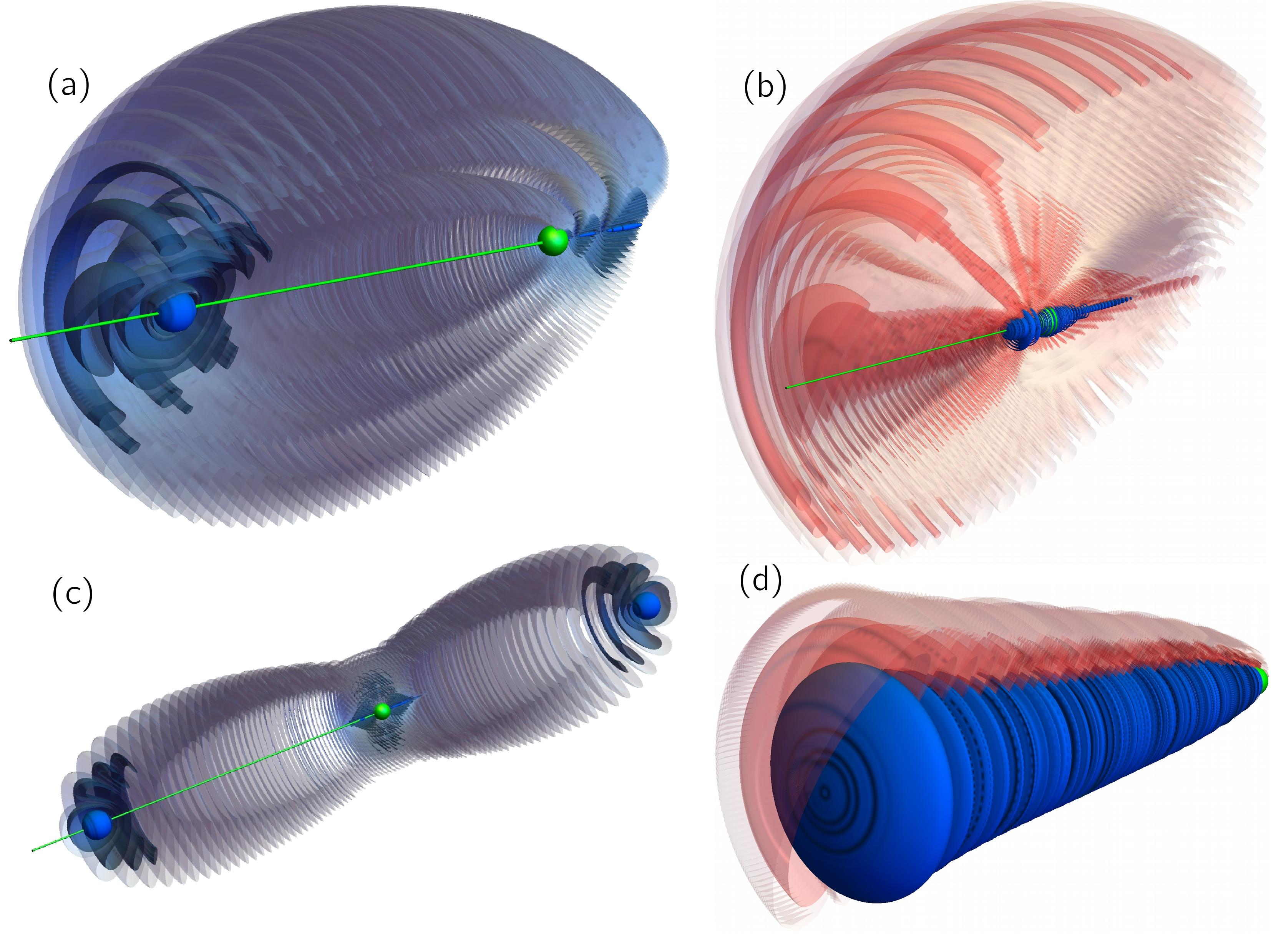
Figure 2: A gallery of trilobite-like ghost bonds for $n=70$, shown as isosurfaces as described in the caption of Fig. 1. (a) A $b=3$ trilobite; (c) an even-parity collinear $b=1$ trilobite trimer. (b) a butterfly with $R_{0}=653$; (d) the deepest Stark state.

The preparation of these exotic chemical bonds hinges on the fact that Rydberg electrons are strongly affected by external fields. These can manipulate the wave function into classical wave packets Parker and Jr (1986) or long-lived circular states Hulet and Kleppner (1983); Signoles et al. (2017). The enormous extent of Rydberg wave functions creates large transition dipole matrix elements, facilitating easy control even with weak field strengths. The Stark and quadratic Zeeman matrix elements scale as $Fn^{2}$ and $B^{2}n^{4}$, respectively, where $F$ and $B$ are electric and magnetic field amplitudes Gallagher (2005).

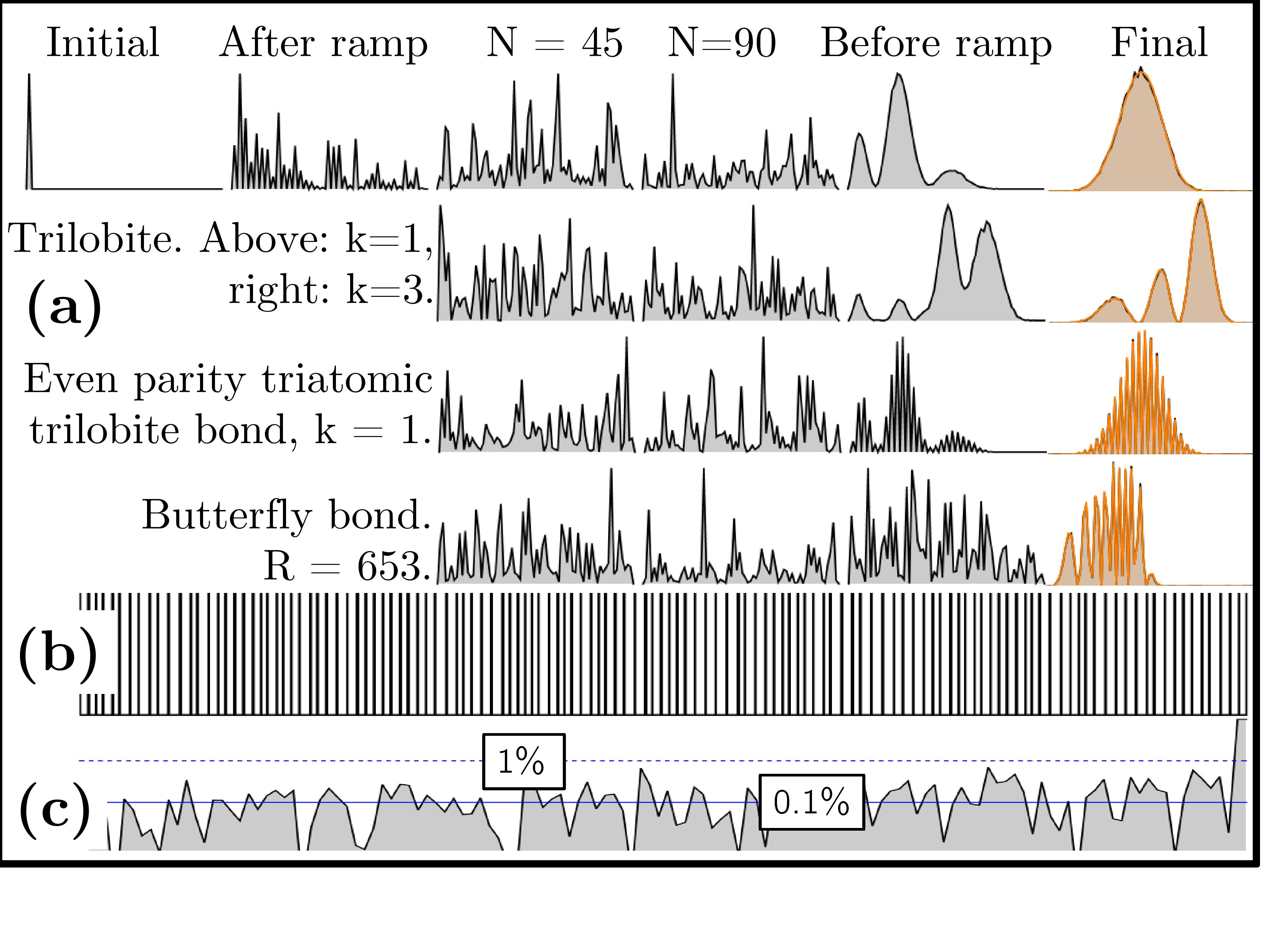
Figure 3: Details of the proposed scheme for the four orbitals shown in Fig 2. a) $l$-distributions, spanning from $l=0$ on the left to $l=69$ on the right, at six different times. The first two times, the initial state and the Zeeman state following the field ramp, are identical in all cases. The orange overlay in the final state shows the exact target distribution. b) The field pulses responsible for this $b=3$ trilobite. The electric fields are turned on in black regions and off in white regions. c) The fidelity, on a logarithmic scale, as a function of time.

The goal of our control scheme is to engineer a final state $\vec{c}_{f}$ which matches the target state, $\vec{c}_{T}$. Their similarity is characterized by the fidelity $\Phi=|\langle\vec{c}_{T}|\vec{c}_{f}\rangle|^{2}$. After choosing the field amplitudes and initial ramp times the final state is determined by the $2N$ time periods: $\Delta t_{i}^{f}$, when both fields are on, and $\Delta t_{i}^{b}$, when only the magnetic field is on. Although square pulses are used for simplicity in the present calculations, the error of a finite ramp time in an experiment should still be within the tolerance of our ideal parameter scheme, and a more thorough calculation could certainly include arbitrary pulse shapes to better match experimental conditions. A gradient ascent algorithm finds optimal $\Delta t_{i}^{b,f}$ parameters giving local maxima in $\Phi$ remarkably efficiently. Numerical experiments reveal several generic features of this approach. First, every optimal pulse sequence is primarily determined by the distribution of initial values, typically drawn from a uniform distribution of experimentally realistic values. This implies that there are effectively infinitely many good pulse configurations. One of these is shown in Fig. 3b, and a full data table of this sequence along with others which create the other chemical bonds in Fig. 2 is given in the supplementary material Note (1). The non-uniqueness of the solutions implies that $\Phi$ is not convex, so there is no guarantee that a gradient ascent algorithm will discover global maxima. Surprisingly, our simulations found that, provided enough pulses (typically $N\approx 2n$) of adequate duration ($\sim 10$s of ns) are used, almost all sequences gave $\Phi>0.999$. Finally, methods that attempt to increase the fidelity monotonically with each pulse appear impossible. Fig. 3 c shows $\log_{10}\Phi$: at no time prior to the final step of evolution does the fidelity increase above 0.01, nor is it monotonically increasing.

These findings are corroborated by optimal control theory Brif et al. (2010). Quite general quantum proofs exist demonstrating that the topology of quantum control landscapes are very favorable to simple extrema search algorithms Demiralp and Rabitz (1993); Rabitz et al. (2004). Only globally maximal seams exist in a sufficiently large parameter space; local maxima do not exist Chakrabarti and Rabitz (2007); Russell et al. (2017); Moore and Rabitz (2011). It is justifiable to restrict the initial guess to realistic experimental values for the field strengths and durations, rather than directly implementing these constraints into the search algorithm. This works excellently given the incredible flexibility of possible solutions Demiralp and Rabitz (1993); Geremia et al. (2000). The lack of local maxima guarantees that optimal solutions are found rapidly without more complicated genetic algorithms or stochastic optimizers Chakrabarti and Rabitz (2007).

The complex quantum pathways the wave function evolves along necessitate very stringent control over the field amplitudes and pulse timing. The experiment must be very well shielded from stray fields so that the control field amplitudes can be specified to better than 10 $\mu$V/cm and 1 mG. Rydberg atoms themselves can be used as highly sensitive field sensors Facon et al. (2016); Ma et al. (2017). The pulse timing should be controlled to femtosecond precision. These error bounds correspond to a 10% reduction in the fidelity from the theoretical prediction. This sensitivity appears to be intrinsic to high Rydberg states, rather than caused by a poorly informed optimal control theory approach. These high sensitivities may require more precise theoretical methods to compute the time evolution as effects beyond first-order perturbation theory are near to this level of accuracy; the proof of principle demonstrated here is still applicable in more sophisticated approaches. A straightforward improvement could include a a robustness measure as a cost function in the optimization, and then use more sophisticated optimization techniques. Recently this approach successfully obtained optimal radio-frequency pulses to excite circular Rydberg states Patsch et al. (2018), and could similarly ease the experimental difficulties here.

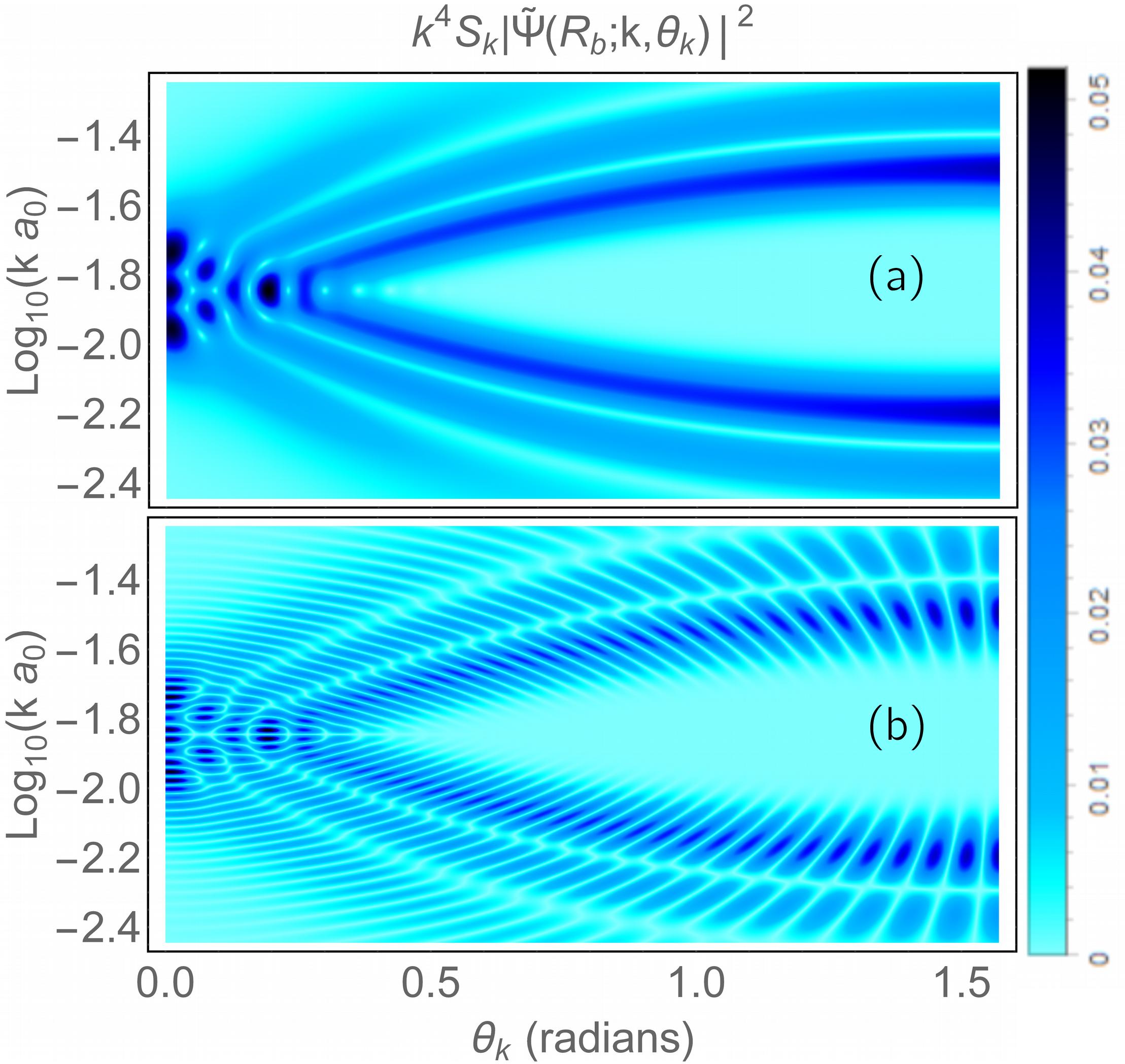
Figure 4: Momentum-space probability distributions for the $n=70$ $b=3$ trilobite dimer (a) and trimer (b). Both are symmetric about $\theta_{k}=\frac{\pi}{2}$ and, when multiplied by $k^{4}$, are logarithmically symmetric about $k=1/n$. The scaling factor $S_{k}=(\theta_{k}+0.1)$ enhances the visibility at large $\theta_{k}$.

Two experimental methods could directly detect the ghost orbital: electron momentum $(e,2e)$ spectroscopy and $x$-ray diffraction Note (1). In $(e,2e)$ spectroscopy an energetic electron scatters from and ejects the Rydberg electron; both are detected in coincidence Brion et al. (2001a); Coplan et al. (1994); Brion et al. (2001b). If the electron-electron collision is fully elastic–requiring large momenta, energies exceeding the ionization potential, and large momentum transfer between the electrons–the triply differential cross section is proportional to the electron’s momentum density Brion et al. (2001a, b). Typically only spherically averaged cross sections can be measured in isotropic samples, but since these trilobite-like orbitals are aligned in the direction of the control fields the fully differential cross section can be measured.

Figure 5: The quantity $\left|k^{2}F_{T}\left(R_{b};\vec{k}\right)\right|$ for the $n=30$ $b=1$ and $b=3$ trilobites. The scaling factor $k^{2}$ is added to improve visibility of small features. This function is also symmetric about $\theta_{k}=\frac{\pi}{2}$. $n=30$ was chosen to connect back to the very first trilobite molecule prediction Greene et al. (2000).

A complementary technique is $x$-ray diffraction James (1982). The differential scattering cross section for this process is proportional to the Fourier transform of the electron density itself, creating another window into the electronic structure of these ghost orbitals. Figs. 4 and 5 show these two different quantities–the momentum density and the Fourier-transformed position density, respectively–for several example ghost orbitals. As expected from Fourier analysis, the momentum-space wave functions in Fig. 4 mirror the symmetries and nodal structure present in the real-space wave functions. Three ridges mirror the nodes in the $b=3$ trilobite, and the even-parity trimer possesses additional nodes overlapping these ridges showing the absence of odd-parity components. The symmetries in $\theta_{k}$ and $k$ relate to the symmetry of the real-space wave function. The Fourier-transformed electron density has many of these same features, although it is no longer symmetric about $k=1/n$. It is also significantly smaller in magnitude and less clear to interpret, although the major nodal features corresponding to the trilobite lobes are still apparent Note (1).

This letter discussed how exotic ultra-long-range ghost chemical bonds consisting of just one atom could be formed and detected in the laboratory. The electron can be either forced to localize very tightly on one or more positions in space, as in the “trilobite”, or to spread out into an exotic fan-like structure, as in the “butterfly”. The control scheme, consisting of a slowly varying magnetic field along with a sequence of rapidly pulsed electric fields, emulates the Fermi pseudopotential responsible for the formation of Rydberg molecules by neutral perturbers. The specifics of the field timings are designed efficiently using a gradient ascent algorithm, and excellent fidelity ($\gg 99.9\%$) can be reached with typical laboratory fields and time scales. The stringent control constraints on the field amplitudes and pulse timings, requiring excellent shielding towards stray fields and knowledge of field strengths to high accuracy, are certainly major experimental hurdles reflecting the exaggerated energy scales and complexity of this system, a novel regime for optimal control theory. One can envision even more exotic ghost states for future study, such as extended configurations like the trimer molecules shown here with several more “ghost” atoms spaced along a line Note (1), or even non-cylindrical polyatomic orbitals (requiring $m_{l}\neq 0$ contributions also).“Electron lattices” could even be envisioned where wave function peaks are placed regularly around the atomic core, with potential applications in quantum gate technology. The theory could be likewise extended to atoms with quantum defects or performed more accurately to include nonperturbative field effects. The proposed detection methods are equally applicable to real Rydberg molecules Shao and Starace (2013); Dixit et al. (2012).

Supplemental Information

I introduction

This supplementary material provides more information about the evolution of the wave function, the detection schemes, and the relevant physical parameters for a realistic implementation. It also provides the actual pulse durations, $\Delta t_{i}^{f}$ and $\Delta t_{i}^{b}$, used for the figures in the main text. Additional figures showing the correspondence between position and momentum representations of the wave functions are also given.

II Time Evolution

We describe the time evolution caused by these time-dependent field pulses using degenerate first-order perturbation theory. The electronic wave function is expanded into the degenerate stationary Rydberg states of a given $n$ with time-dependent coefficients: $\Psi(\vec{r},t)=\sum_{l}c_{l}(t)\phi_{nl}(\vec{r})$. In a parallel field configuration $m_{l}$ is still a good quantum number, so we consider only the $m_{l}=0$ subspace. In a time period $\Delta t_{i}^{b}$ when the electric field is zero, the Hamiltonian is $H_{B}=H_{0}+\frac{B^{2}}{8}r^{2}\sin^{2}\theta$. Likewise, when the electric field is nonzero for a time period $\Delta t_{i}^{f}$, $H_{F}=H_{B}+Fr\cos\theta$. In the degenerate subspace of a single $n$ manifold, the action of $H_{0}$ is irrelevant and can be set to zero; the operators $H_{B}$ and $H_{F}$ are then diagonalized to obtain the diagonal eigenvalue matrices $\underline{b}$, $\underline{f}$ and eigenvector matrices $\underline{U_{b}}$, $\underline{U_{f}}$, respectively. The integrals involved in finding the matrix elements of $H_{B}$ and $H_{F}$ are

$$\langle l|\cos\theta|l^{\prime}\rangle =\sqrt{\frac{(l_{<}+1)^{2}}{(2l_{<}+1)(2l_{<}+3)}}\delta_{l,l^{\prime}\pm 1},$$ (S1)

$$\langle l|\sin^{2}\theta|l^{\prime}\rangle =\frac{2(l^{2}+l-1)}{(2l+3)(2l-1)}\delta_{ll^{\prime}}-\sqrt{\frac{(l_{<}+2)^{2}(l_{<}+1)^{2}}{(2l_{<}+5)(2l_{<}+3)^{2}(2l_{<}+1)}}\delta_{l,l^{\prime}\pm 2},$$

$$\langle nl|r^{k}|n^{\prime}l^{\prime}\rangle =\frac{2^{l+l^{\prime}+2}}{n^{l+2}n^{\prime l^{\prime}+2}}\sqrt{\frac{(n-l-1)!(n^{\prime}-l^{\prime}-1)!}{(n+l)!(n^{\prime}+l^{\prime})!}}$$ (S2)

$$\times\sum_{m,m^{\prime}=0}^{m=n-l-1}\begin{pmatrix}n+l\\ n-l-1-m\end{pmatrix}\begin{pmatrix}n^{\prime}+l^{\prime}\\ n^{\prime}-l^{\prime}-1-m^{\prime}\end{pmatrix}\frac{(k+m+m^{\prime}+l+l^{\prime}+2)!}{\left(\frac{n+n^{\prime}}{nn^{\prime}}\right)^{k+3+l+l^{\prime}+m+m^{\prime}}},$$ (S3)

where $()$ are binomial coefficients. A derivation of the radial matrix element can found in Dong et al. (2004).

During each $\Delta t$ the Hamiltonian is time-independent, so the evolution of the initial state is computed by iteratively acting on it with the unitary time evolution operator for each pulse until the final time is reached:

$$\vec{c_{f}} =\underline{X_{B}}^{\dagger}\left[\prod_{i=1}^{N}\underline{U_{b}}e^{-i\Delta t_{i}^{b}\underline{b}}\underline{U_{b}}^{-1}\underline{U_{f}}e^{-i\Delta t_{i}^{f}\underline{f}}\underline{U_{f}}^{-1}\right]\underline{X_{B}}\vec{c_{0}}.$$ (S4)

$X_{b}=\underline{U_{b}}e^{-i\Delta t_{\text{ramp}}\underline{b}}\underline{U_{b}}^{-1}$ is the field ramp operator.

Unlike many problems where major effort is needed to numerically calculate the gradient Khaneja et al. (2005), in the present case the gradient is given analytically (without loss of generality here is the partial derivative with respect to $\Delta t_{j}^{f}$):

$$\frac{\partial\Phi}{\partial\Delta t_{j}^{f}} =\left\langle\frac{\partial\vec{c_{f}}}{\partial\Delta t_{j}^{f}}\right|\vec{c_{T}}\Bigg{\rangle}\langle\vec{c_{T}}|\vec{c_{f}}\rangle+\text{c.c.}$$ (S5)

$$\frac{\partial\vec{c_{f}}}{\partial\Delta t_{j}^{f}} =\underline{X_{B}}^{\dagger}\Bigg{[}\prod_{i=1}^{N}\underline{U_{b}}e^{-i\Delta t_{i}^{b}\underline{b}}\underline{U_{b}}^{-1}\underline{U_{f}}\left(-i\underline{f}\right)^{\delta_{ij}}e^{-i\Delta t_{i}^{f}\underline{f}}\underline{U_{f}}^{-1}\Bigg{]}\underline{X_{B}}\vec{c_{0}}.$$ (S6)

After finding this gradient, the full set of parameters $\{\Delta t_{i}^{O}\}$ is shifted in the direction of the steepest change in the fidelity, $\Delta t_{i}^{O}\to\Delta t_{i}^{O}+\varepsilon\frac{\partial{\Phi}}{{\partial\Delta t_{i}^{O}}}$, where $\varepsilon$ is a variable stepsize and $O$ represents either $f$ or $b$.

III Physical considerations for the control scheme

Relativistic effects
The fine structure breaks the exact degeneracy of $nl$ states with low $l$. The $70p_{1/2,3/2}$ ($70d_{3/2,5/2}$) levels are split by $\approx 0.25(0.085)$ MHz. Precession between different $m_{l}$ states caused by the $np$ splitting over the time scale of the experiment introduces undesirable decoherence. To avoid this problem a magnetic field of 100G is applied to access the Paschen-Back regime and eliminate this precession by energetically separating $m_{l}\neq 0$ levels.
Magnetic fields
These relatively large magnetic fields are also necessary since the quadratic Zeeman term is very small compared to the linear Stark shift. It is challenging experimentally to change fields of this strength quickly due to the self-inductance of the electronics. We have adopted the slew rate 10G/5$\mu$s of state of the art magnetic field coils developed to quench ultracold atomic species Makotyn (2014).
Pulse sequence and field strength parameters
There is considerable flexibility in the initially guessed pulse distribution. The simplest theoretical choice is simply to draw the initial distribution randomly from a region of experimentally realistic values. The range of these values should be limited to reduce the overall time. The optimized field pulses then closely mirror this initial distribution due to the incredible multiplicity of optimal configurations and their sensitivity. Sequences leading to very good fidelity can also be found with an initial configuration of equal-duration pulses, although with somewhat more difficulty since the parameter space is less robust. Setting $N=130$ essentially guaranteed $\Phi>0.999$ regardless of the initial distribution, while for $N=120$ high fidelities $\Phi\approx 0.99$ were always achieved but $\Phi>0.999$ was not. For $N$ even as low as 70 $\Phi\approx 0.9$ reliably. Likewise the field amplitudes can be adjusted to better conform to a specific experiment. The magnetic field amplitude should be fairly large, as described above, while the electric field amplitude should not be large enough that different Rydberg levels together can mix together. For $n=70$ this restricts it to not far exceed the 0.1V/cm employed here.
Rydberg levels
High principal quantum numbers are needed to ensure that the above constraints are sufficient, but also increase the theoretical complication and experimental limits on sensitivity. The benefits are contingent on various Rydberg scaling laws: the fine structure splitting decreases as $\mathcal{O}(n^{-3})$, magnetic field effects increase as $\mathcal{O}(n^{4})$, and the natural and blackbody radiative decay rates decrease as $\mathcal{O}(n^{-3})-\mathcal{O}(n^{-5})$ (depending on $l$) and $\mathcal{O}(n^{-2})$, respectively. The number of pulses and electric field influence increase as $\mathcal{O}(n)$ and $\mathcal{O}(n^{2})$, respectively, and the electron’s momentum decreases as $\mathcal{O}(n^{-1})$; the sensitivity to error and difficulty of detection are thus increased at high $n$. Additionally, first-order perturbation theory starts to become less accurate at higher $n$ due to the decreasing (as $\mathcal{O}(n^{-3})$) separation between Rydberg manifolds. $n=70$ functions in our exemplary calculations as a convenient middle ground, but the wide range of theoretical and experimental constraints mean that this choice is quite flexible depending on the circumstances.
Calculation details
The specific field configurations for the orbitals in Fig. 1 in the main text are presented in table 1. We chose $n=70$, $B_{max}=100$G, $F_{max}=0.1$V/cm, and $N=130$. $\Delta t_{i}^{b}$ and $\Delta t_{i}^{f}$ were chosen randomly from the ranges $\{200,400\}$ and $\{20,60\}$ns, respectively. The ability to of the gradient ascent algorithm within this scheme to find optimal solutions is surprisingly robust to variations of all these parameters. Scaling laws can also be used to vary the parameters. The system is invariant under the transformations $F\to\mathcal{F}$, $B\to B\sqrt{\mathcal{F}/F}$, $\Delta t_{i}^{O}\to\Delta t_{i}^{O}(F/\mathcal{F})$, and $T_{\text{ramp}}\to T_{\text{ramp}}(F/\mathcal{F})^{3/2}$.
Orbital details
The (unnormalized) final state coefficients are given by:Eiles et al. (2016); Chibisov et al. (2000); Khuskivadze et al. (2002).

$$c_{nl,trilobite}^{b} =\phi_{nl0}(R_{b})$$ (S7)

$$c_{nl,butterfly}^{b} =\frac{\partial\phi_{nl0}}{\partial R_{b}}$$ (S8)

$$c_{nl,even/oddparitytrimer}^{b} =\frac{(1\pm(-1)^{l})}{\sqrt{2}}c_{nl,x}^{b}$$ (S9)

evaluated at the bond positions $R_{b}$ which are determined for each state by finding the minima of $\sum_{l}|c_{nl,x}^{b}|^{2}$.

The momentum-space wave function for a trilobite-like orbital characterized by coefficients $c_{nl,x}^{b}$ is

$$\tilde{\Psi}(R_{b};\vec{k}) =\frac{\sum_{l=l_{0}}^{l=n-1}c_{nl,x}^{b}F_{nl}(k)Y_{l0}(\theta_{k},\phi_{k})}{\left(\sum_{l=l_{0}}^{n-1}|c_{nl,x}^{b}|^{2}\right)};$$

$$F_{nl}(k) =-(-i)^{l}\sqrt{\frac{2(n-l-1)!}{\pi(n+l)!}}n^{2}2^{2(l+1)}l!n^{l}k^{l}$$

$$\times(n^{2}k^{2}+1)^{-l-2}C_{n-l-1}^{l+1}\left(\frac{n^{2}k^{2}-1}{n^{2}k^{2}+1}\right),$$

where $C_{i}^{j}$ is the Gegenbauer polynomial of degree $i$ and order $j$; these “radial” momentum space wave functions were calculated shortly after the first solution of the quantum mechanical hydrogen atom Podolsky and Pauling (1929). They possess a symmetry under the change of variables $nk=a^{x}$, where $a$ is some constant. For simplicity, if $a$ is $e$,

$$F_{nl}(x)=-(-i)^{l}\sqrt{\frac{2(n-l-1)!}{\pi(n+l)!}}n^{2}2^{2(l+1)}l!n^{l}k^{l}e^{-2x}(\sinh(x))^{-l-2}C_{n-l-1}^{l+1}\left(\tanh(x)\right),$$ (S10)

From inspection this function possesses a mirror symmetry (odd or even depending on the parity of $n$) about $x=0$ when multiplied by $e^{2x}$. This is the reason for the symmetry about $k=1/n$ of the function $|k^{2}\Psi(k)|^{2}$.

IV Further details about detection methods and momentum-space densities

There are two additional detection techniques, involving field ionization, that could be employed instead of the two discussed in the main text. In Stark photoionization spectroscopy, the electron is photoionized and detected on a distant screen. This maps the real-space electron wave function into Stark states, but unfortunately the theoretical description and extraction of the wave function’s properties is too imposing for this to be a robust and clear method in the present context Cohen et al. (2016); Zhao et al. (2012); Giannakeas et al. (2015). A related, but more straightforward, technique is ionization by half-cycle pulses Robicheaux (1997); Jones (1996). A half-cycle pulse along the $z$ axis imparts a momentum kick to the Rydberg electron, and if the electron’s increased energy is sufficient to overcome the ionization potential it will be detected. A measurement of the electron current is therefore proportional to $\int_{k_{z}}^{\infty}\int_{k_{x},k_{y}}|\Psi(\vec{k})|^{2}\mathrm{d^{3}}{k}$, where $\vec{k}$ is the momentum of the electron. A very similar observable is obtained in Compton scattering Cooper (1985). $k_{z}$ is determined by the momentum kick, so by varying this the probability density that the electron had momentum $k_{z}$ and any value of $k_{x}$ and $k_{y}$ can be obtained. Although the simplicity of this approach is attractive, much of the detailed structure of the wave function is averaged over and obscured.

The advantage of both techniques we focused on in the main text is that they, in principle, can lead to direct measurements of the electron’s spatial properties, specifically either its momentum density or the Fourier transform of its real-space density. Here we provide additional details of these two techniques. In $(e,2e)$ spectroscopy, an electron with momentum $\vec{k}_{0}$ collides with the Rydberg electron, which has momentum $\vec{k}$. Both elastically scatter into plane waves with momenta $\vec{k}_{a}$ and $\vec{k}_{b}$, and are detected in coincidence. The triply-differential cross section for this process is Brion et al. (2001a); Coplan et al. (1994); Brion et al. (2001b)

$$\frac{d^{3}\sigma_{(e,2e)}}{d\Omega_{a}\Omega_{b}dE_{b}}=\frac{4k_{a}k_{b}}{k_{0}|\vec{k}_{0}-\vec{k}_{a}|^{4}}\left|\tilde{\Psi}(R_{b};\vec{k})\right|^{2},$$ (S11)

where $\Omega_{i}$ is the solid angle in which electron $i$ is detected, and $E_{b}$ is the energy of electron $b$. There are many commonly used experimental geometries which determine the specific form of the kinematic factor $|\vec{k}_{0}-\vec{k}_{a}|^{-4}$ and the relationship between $\vec{k}$, $\vec{k}_{a}$, and $\vec{k}_{b}$. Depending on the implementation, the angle of incident electrons or their initial energy can be tuned to vary $\vec{k}$. We have focussed on the key features of the momentum density, since this gives the properties of the Rydberg electron that we want to study, and the kinematic properties can then be optimized by the preferred choice of geometry.

The differential scattering probability for $x$-ray diffraction is given by James (1982)

$$\frac{d\sigma}{d\Omega}=\frac{d\sigma_{th}}{d\Omega}\left|\int\left|\Psi(R_{b},\vec{r})\right|^{2}e^{i\vec{k}\cdot\vec{r}}\mathrm{d^{3}}{r}\right|^{2},$$ (S12)

where $\frac{d\sigma_{th}}{d\Omega}$ is the Thomson cross section. The Fourier transform of the electronic density is more involved than the calculation of the momentum wave functions. We proceed in the usual fashion, expanding the plane wave into spherical harmonics:

$$\int\mathrm{d^{3}}{r}e^{i\vec{k}\cdot\vec{r}}|\Psi(R_{k},\vec{r})|^{2} =\sum_{l,k,p}\int\mathrm{d^{3}}{r}c_{l}c_{k}4\pi i^{p}j_{p}(kr)u_{nl}(r)u_{nk}(r)Y_{l0}(\hat{r})Y_{k0}^{*}(\hat{r})Y_{p0}^{*}(\hat{r})Y_{p0}(\hat{k})$$

$$=4\pi\sum_{l,k}c_{l}c_{k}\sum_{p=|l-k|}^{p=l+k}i^{p}\sqrt{\frac{(2l+1)(2p+1)(2k+1)}{4\pi}}\begin{pmatrix}l&p&k\\ 0&0&0\end{pmatrix}^{2}\int\mathrm{d}{r}j_{p}(kr)u_{nl}(r)u_{nk}(r)Y_{p0}(\hat{k}).$$

Here $c_{l},c_{k}$ are the coefficients determining the orbital state. This radial integral can be evaluated in terms of hypergeometric functions following Eq. 40 of Ref. Shao and Starace (2013).

Figure S1: Position-space Rydberg molecule wave functions, plotted in cylindrical coordinates. a) $b=1$ trilobite; b) $b=3$ trilobite; c) $b=1$ trilobite trimer; d) $b=3$ trilobite trimer; e) $b=48$ trilobite; f) butterfly; g) stark state; h) $b=1$ trilobite, 84% match.

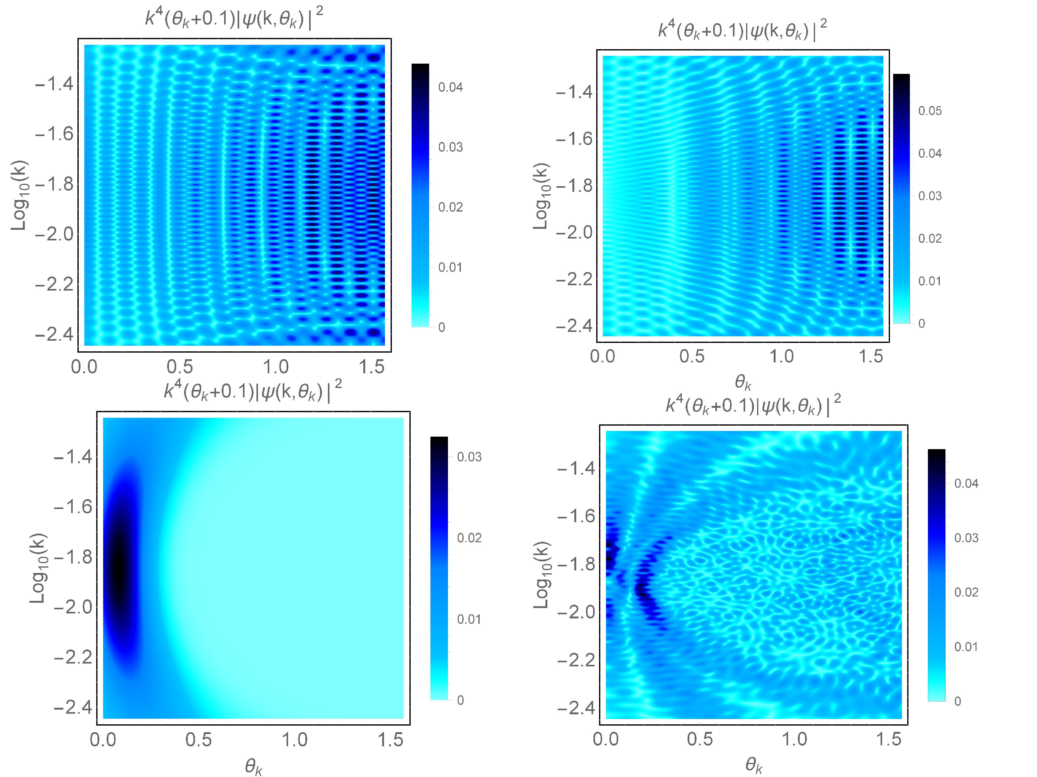
Figure S2: Momentum-space Rydberg molecule wave functions, plotted in spherical coordinates. a) $b=1$ trilobite; b) $b=3$ trilobite; c) $b=1$ trilobite trimer; d) $b=3$ trilobite trimer; e) $b=48$ trilobite; f) butterfly; g) stark state; h) $b=1$ trilobite, 84% match.

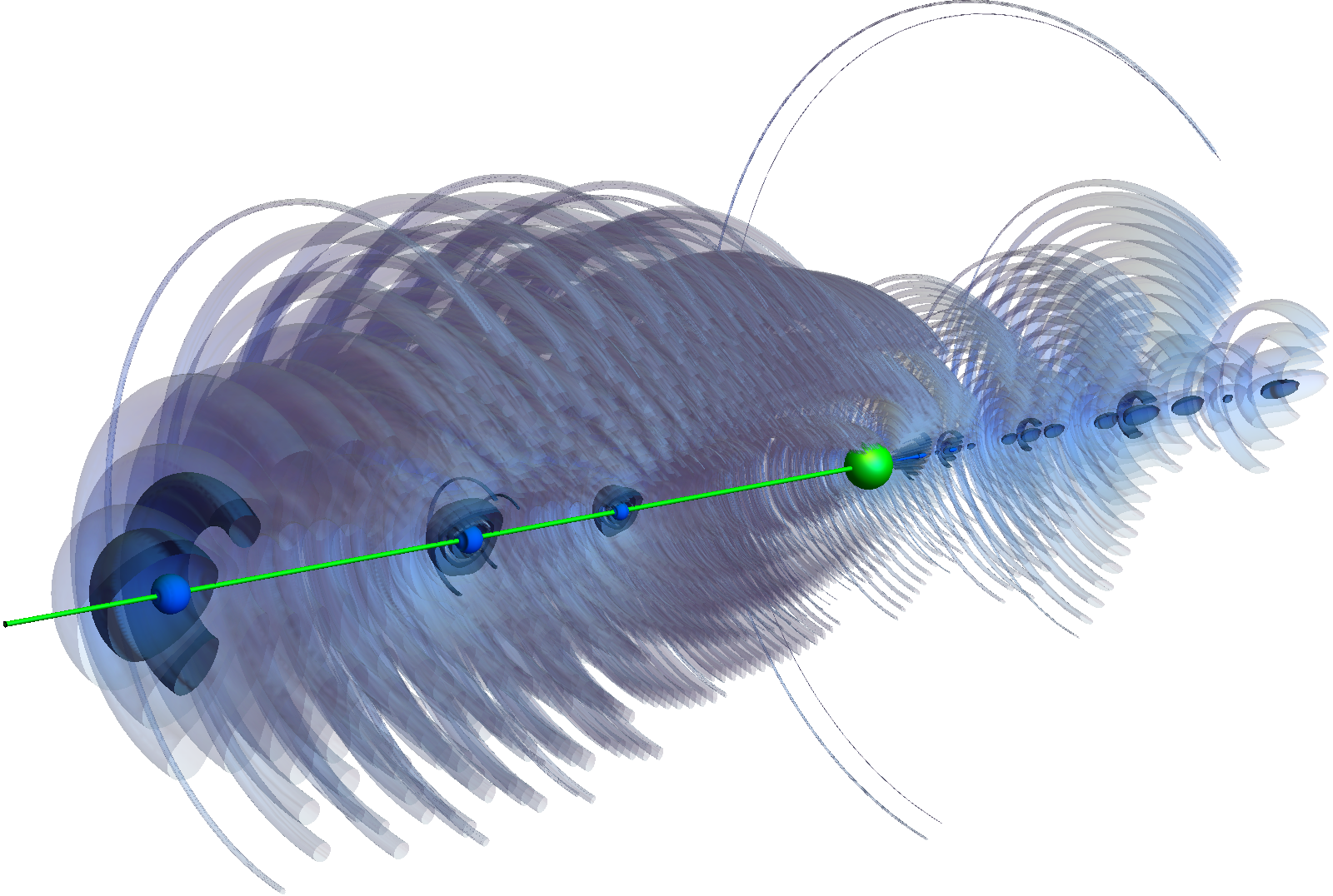
Figure S3: Even more unusual variants can be formed following this same scheme, such as this case with three electron peaks placed along an axis. The color scheme is the same as in the main text, with the small bright blue regions having 10X the amplitude as the darker blue, and 100X the amplitude as the prominent gray regions.

V Data tables

130-pulse sequences to make 99.9% molecular bonds such as those shown in the first two figures in the main text.

$k=1$	(1-65)	(66-130)	143649	$k=3$	(1-65)	(66-130)	144631	trimer	(1-65)	(66-130)	144583	btfly	(1-65)	(66-130)	144578
36.0129	239.973	32.2792	224.897	30.6755	285.278	28.2444	295.56	35.4941	317.394	34.9943	371.849	60.3706	367.018	60.7922	228.261
47.4666	296.119	34.6906	224.662	59.6629	244.097	58.1024	266.409	41.2067	227.01	61.6375	330.277	39.8348	200.876	58.1241	242.571
30.0045	371.947	52.899	399.063	22.901	227.233	32.7547	254.69	37.1052	359.677	24.865	352.076	26.4902	305.972	38.5931	399.63
26.9364	305.557	32.3173	369.321	43.4052	329.984	57.4415	252.275	22.7512	274.308	53.14	250.2	59.5579	220.389	45.8705	378.874
48.2474	390.364	21.6446	326.888	46.8757	205.56	57.1991	327.417	43.174	316.964	45.5835	343.93	35.2915	219.911	42.8275	286.915
35.3907	286.297	49.5366	256.09	52.8709	362.685	30.79	381.279	52.2115	320.772	31.6169	316.027	28.1597	206.653	36.5052	366.661
30.4024	323.885	39.0652	315.117	36.9635	298.669	26.7545	357.504	44.5726	303.069	30.7177	327.868	54.4036	259.798	36.5816	335.232
56.3999	209.329	44.7074	381.198	20.7992	395.597	23.3285	395.421	30.6065	352.557	50.4794	213.035	24.8793	296.894	25.1104	357.093
45.9804	236.636	21.7709	326.225	39.8652	274.949	46.741	383.931	30.5509	315.958	52.9686	292.449	43.5578	313.587	40.7838	328.844
21.4295	335.036	57.9015	352.016	29.2127	373.025	56.8444	210.272	54.4517	295.954	30.9039	355.396	56.7162	245.521	35.0073	236.966
22.8669	367.902	54.4536	290.009	48.6238	397.661	32.1329	370.697	58.3629	329.656	38.9009	376.617	37.5066	220.36	19.574	365.431
32.0231	383.247	31.783	255.278	58.3326	345.844	21.8744	356.343	50.6946	376.125	55.3135	335.137	20.4112	393.853	35.8386	321.852
60.2675	265.296	48.1839	315.093	45.4129	202.377	47.0193	276.46	38.8064	228.696	49.6757	363.387	40.9484	363.069	45.881	268.174
38.8887	223.329	60.4721	250.07	51.7152	395.18	46.6587	288.208	32.8958	319.173	32.5454	251.306	51.8996	363.292	33.9069	373.105
58.0465	334.239	48.1055	212.31	22.0069	341.64	41.3305	210.498	50.8416	340.081	47.9297	280.926	39.7599	249.473	33.4779	207.189
57.5267	389.306	35.8335	217.65	26.2229	242.293	41.0315	299.244	49.1342	238.827	34.8307	273.306	57.2002	399.043	34.7687	222.04
23.5209	394.01	38.2097	201.5	50.2489	299.515	23.5623	219.671	30.9119	200.408	44.5811	278.972	32.0786	282.291	29.7687	305.958
54.5002	295.453	29.6287	285.938	54.3202	286.47	43.2787	296.826	22.971	226.089	35.117	337.097	32.5831	322.687	37.8944	305.699
39.4703	206.331	32.3441	258.172	56.3983	307.395	24.8648	379.713	24.3993	219.168	43.812	236.388	20.0271	361.559	47.3182	360.582
56.7084	256.443	30.9668	263.233	55.9024	259.512	29.4882	202.415	52.3659	334.999	28.1357	246.272	27.731	272.172	34.3291	340.796
28.0783	230.737	46.2487	379.572	31.1048	200.4	53.7477	385.433	22.6289	341.545	58.1248	365.036	35.2022	338.487	34.9558	330.768
27.4159	360.588	54.245	337.983	39.6045	336.299	58.7858	351.59	36.6224	348.738	55.4131	282.814	40.0481	338.553	36.2144	356.28
28.0018	209.663	51.2241	254.757	26.7141	204.882	56.6222	247.432	50.4774	308.945	48.6759	227.929	30.2489	326.799	36.7335	264.212
41.1562	375.336	54.7605	249.41	41.1233	273.923	46.0954	381.257	28.8492	242.746	29.9056	268.698	24.4098	216.463	37.3114	275.256
23.6961	269.633	45.594	358.763	32.4852	281.958	35.3781	388.049	40.7027	235.288	42.5593	229.814	37.4246	291.68	55.8091	232.417
44.193	239.039	21.8992	259.108	38.1478	384.26	48.7241	396.525	26.8742	378.235	35.1144	352.779	33.0148	326.247	44.7961	248.977
46.8809	266.353	26.2047	314.306	32.0011	217.978	31.4193	296.609	47.0053	242.595	55.8567	205.326	21.356	256.536	22.7177	360.936
27.4893	233.389	60.5374	213.329	55.9752	288.14	51.5617	357.951	56.9714	333.463	55.9697	277.301	58.0937	307.07	36.4336	375.12
59.4849	241.986	22.2376	380.693	59.7606	348.423	26.5195	371.158	37.708	392.821	28.0426	252.5	35.9571	239.647	45.9658	304.406
22.6778	288.645	23.7563	237.295	51.8483	352.026	34.3525	300.214	53.9524	229.21	39.4129	295.992	49.3244	278.39	30.0952	379.697
31.5342	215.259	38.1811	364.905	24.84	351.879	54.7173	234.761	37.2985	219.555	37.558	383.275	34.4936	291.086	41.2862	314.257
47.0625	292.209	20.9276	246.949	58.3077	268.378	31.1896	369.958	53.0096	238.627	36.2796	220.377	50.1296	297.785	40.6829	232.539
36.8888	382.182	29.8878	378.93	44.0284	278.645	44.8019	269.558	26.9275	247.854	58.1631	326.799	23.9885	365.504	38.6288	225.26
21.9193	280.661	24.6508	282.762	41.7882	298.654	31.932	220.334	54.7396	250.558	33.0521	318.584	51.5307	296.675	22.5173	342.054
20.2117	368.671	34.157	345.272	32.4352	262.323	23.4262	334.959	31.6746	364.349	42.9386	392.974	53.9926	233.198	40.3963	241.13
34.0221	384.654	27.9355	250.431	45.3283	316.765	22.251	235.589	46.3985	339.204	45.9787	238.165	39.6537	279.727	25.4145	289.824
43.1697	352.925	39.9112	305.71	58.4723	232.633	25.6947	327.89	26.5834	342.254	46.7611	259.763	50.0239	353.974	47.5152	216.052
32.9205	270.138	53.0118	375.556	57.6169	314.096	26.5022	277.831	48.5323	282.514	26.0348	330.627	27.7551	222.77	42.6354	267.576
37.0737	212.815	39.453	368.708	46.1446	285.484	52.1491	257.077	52.9682	337.359	25.494	303.908	37.3639	374.937	49.3535	312.226
43.3936	367.695	37.5166	364.99	26.4938	306.158	54.108	305.788	48.049	398.049	45.5871	228.933	39.1577	220.815	25.2979	246.669
55.2011	366.178	26.5726	309.188	45.6729	399.616	58.3289	297.998	25.9886	242.361	36.7109	227.367	55.7195	354.727	33.6709	268.085
27.6309	260.188	45.2975	263.423	42.7266	348.977	32.0211	208.119	48.9908	325.304	47.0478	287.425	39.606	278.581	42.3664	274.643
42.9364	333.198	36.1652	214.373	35.4476	213.432	36.2285	260.191	30.7462	286.924	54.5021	350.246	40.0968	216.426	39.8083	295.178
40.0133	259.606	28.0009	273.357	30.2824	274.801	43.815	346.334	37.7796	360.876	30.659	258.053	46.6367	301.11	39.2659	273.952
33.0666	218.466	22.2618	341.86	40.8836	346.152	50.3911	387.497	59.8862	332.371	47.8343	344.693	46.8011	239.983	22.707	337.213
54.7871	373.83	33.7303	399.873	41.4858	328.858	34.361	327.299	25.0457	351.478	24.1661	205.396	23.2958	298.147	23.9924	398.095
54.3451	397.18	22.9229	224.574	53.4793	384.304	27.7848	291.853	24.7318	292.757	49.4903	319.222	49.2207	319.552	29.7442	319.683
57.8814	328.957	46.1466	327.839	56.6214	216.886	36.1084	210.678	37.0623	271.255	26.2631	213.913	31.7887	300.338	53.9314	372.497
31.5916	346.092	53.2207	213.49	40.233	264.668	38.8696	301.498	51.1656	246.016	39.0814	269.016	56.8078	283.341	45.7196	326.861
24.6633	231.851	46.8305	234.938	47.705	242.544	34.5773	389.282	50.2561	352.668	45.4389	345.164	43.4683	365.088	40.0147	381.293
54.3504	261.233	50.3357	344.638	29.0366	231.35	46.7124	363.397	36.3142	265.519	39.3281	396.8	40.7234	362.227	52.517	348.404
32.1983	389.8	36.9001	331.687	21.2776	223.807	32.3433	329.799	41.0068	275.675	26.0152	377.603	49.116	310.698	55.5193	380.661
22.6872	274.048	29.8008	215.523	28.3009	381.216	45.6109	352.837	55.9664	386.452	52.1098	221.565	33.4176	330.421	51.5434	322.372
43.4619	358.925	50.3533	207.864	19.7572	305.762	46.3676	378.444	29.6656	316.855	43.691	309.508	35.0741	336.073	25.6841	326.033
28.8527	252.449	52.4104	221.434	56.604	202.659	28.8499	233.439	34.2256	390.769	49.2657	312.438	27.3429	212.455	24.8583	251.831
39.4534	305.38	52.7095	205.81	21.9487	236.969	59.5223	366.226	38.1006	283.029	25.9424	387.424	44.9696	387.841	25.2758	266.513
30.43	241.009	21.9003	237.052	55.7136	306.774	22.2856	350.021	51.914	309.416	19.6119	290.035	37.1665	381.029	56.1465	274.791
27.3553	332.955	34.6828	332.034	31.3573	365.94	36.114	285.159	34.6322	371.574	53.2117	380.421	25.9724	392.491	29.341	206.092
54.0787	245.303	32.9304	269.907	35.8464	263.302	52.1255	285.945	32.4816	212.59	51.8562	359.448	27.8902	311.855	43.1052	279.411
37.2938	295.502	40.6183	344.606	23.9831	216.722	23.9845	353.351	35.1543	382.07	43.5743	204.431	22.9743	391.437	58.5682	369.634
56.3689	237.913	26.4251	212.98	52.1499	310.168	46.6141	238.038	43.5145	258.071	38.2452	374.988	40.0114	250.353	21.3546	301.212
40.6591	359.133	57.6148	379.082	59.4687	292.52	41.9842	396.399	33.234	209.186	39.4088	262.242	59.7528	316.438	42.0565	381.647
34.8486	322.082	25.6399	396.547	43.7048	375.261	26.1372	330.203	43.1673	337.063	22.405	350.151	20.0563	394.524	22.1436	311.549
52.8148	250.462	31.7913	205.877	35.9426	363.576	39.6143	308.127	29.5018	340.9	49.5556	332.431	22.7972	352.624	41.8479	250.578
55.5378	314.747	49.2313	381.603	59.3795	210.514	22.9112	270.785	29.643	373.777	57.0129	283.93	25.3702	383.803	59.5442	203.046

Table 1: Pulse parameters. Top row: the type of bond (trilobite, $k=1,k=3$; triatomic trilobite with $k=1$; butterfly). Total time, including field ramps (both the up and down ramps last for 50$\mu$s), in nanoseconds. The left column of each is the duration of the electric field pulse, while the right column is the interval in between electric field pulses. 130 pulses are used each time. Times are always in ns.

References

- Dong et al. (2004) S.-H. Dong, C.-Y. Chen, and M. Lozada-Cassou, Physics Letters A 333, 193 (2004).
- Khaneja et al. (2005) N. Khaneja, T. Reiss, C. Kehlet, T. Schulte-Herbrüggen, and S. J. Glaser, Journal of Magnetic Resonance 172, 296 (2005).
- Makotyn (2014) P. Makotyn, Experimental studies of a degenerate unitary Bose gas, Ph.D. thesis, University of Colorado (2014).
- Eiles et al. (2016) M. Eiles, J. Pérez-Ríos, F. Robicheaux, and C. H. Greene, Journal of Physics B: Atomic, Molecular and Optical Physics 49, 114005 (2016).
- Chibisov et al. (2000) M. Chibisov, A. M. Ermolaev, F. Brouillard, and M. H. Cherkani, Phys. Rev. Lett. 84, 45 (2000).
- Khuskivadze et al. (2002) A. A. Khuskivadze, M. I. Chibisov, and I. I. Fabrikant, Phys. Rev. A 66, 042709 (2002).
- Podolsky and Pauling (1929) B. Podolsky and L. Pauling, Phys. Rev. 34, 109 (1929).
- Cohen et al. (2016) S. Cohen, M. M. Harb, A. Ollagnier, F. Robicheaux, M. J. J. Vrakking, T. Barillot, F. Lépine, and C. Bordas, Phys. Rev. A 94, 013414 (2016).
- Zhao et al. (2012) L. B. Zhao, I. I. Fabrikant, M. L. Du, and C. Bordas, Phys. Rev. A 86, 053413 (2012).
- Giannakeas et al. (2015) P. Giannakeas, F. Robicheaux, and C. H. Greene, Phys. Rev. A 91, 043424 (2015).
- Robicheaux (1997) F. Robicheaux, Phys. Rev. A 56, 3358 (R) (1997).
- Jones (1996) R. R. Jones, Phys. Rev. Lett. 76, 3927 (1996).
- Cooper (1985) M. J. Cooper, Rep. Prog. Phys. 48, 415 (1985).
- Brion et al. (2001a) C. Brion, G. Cooper, Y. Zheng, I. Litvinyuk, and I. McCarthy, Chemical Physics 270, 13 (2001a).