Probabilistic FastText for Multi-Sense Word Embeddings

Abstract

We introduce Probabilistic FastText, a new model for word embeddings that can capture multiple word senses, sub-word structure, and uncertainty information. In particular, we represent each word with a Gaussian mixture density, where the mean of a mixture component is given by the sum of n-grams. This representation allows the model to share statistical strength across sub-word structures (e.g. Latin roots), producing accurate representations of rare, misspelt, or even unseen words. Moreover, each component of the mixture can capture a different word sense. Probabilistic FastText outperforms both FastText, which has no probabilistic model, and dictionary-level probabilistic embeddings, which do not incorporate subword structures, on several word-similarity benchmarks, including English RareWord and foreign language datasets. We also achieve state-of-art performance on benchmarks that measure ability to discern different meanings. Thus, the proposed model is the first to achieve multi-sense representations while having enriched semantics on rare words.

1 Introduction

Word embeddings are foundational to natural language processing. In order to model language, we need word representations to contain as much semantic information as possible. Most research has focused on vector word embeddings, such as Word2Vec (Mikolov et al., 2013a), where words with similar meanings are mapped to nearby points in a vector space. Following the seminal work of Mikolov et al. (2013a), there have been numerous works looking to learn efficient word embeddings.

One shortcoming with the above approaches to word embedding that are based on a predefined dictionary (termed as dictionary-based embeddings) is their inability to learn representations of rare words. To overcome this limitation, character-level word embeddings have been proposed. FastText (Bojanowski et al., 2016) is the state-of-the-art character-level approach to embeddings. In FastText, each word is modeled by a sum of vectors, with each vector representing an n-gram. The benefit of this approach is that the training process can then share strength across words composed of common roots. For example, with individual representations for “circum” and “navigation”, we can construct an informative representation for “circumnavigation”, which would otherwise appear too infrequently to learn a dictionary-level embedding. In addition to effectively modelling rare words, character-level embeddings can also represent slang or misspelled words, such as “dogz”, and can share strength across different languages that share roots, e.g. Romance languages share latent roots.

A different promising direction involves representing words with probability distributions, instead of point vectors. For example, Vilnis and McCallum (2014) represents words with Gaussian distributions, which can capture uncertainty information. Athiwaratkun and Wilson (2017) generalizes this approach to multimodal probability distributions, which can naturally represent words with different meanings. For example, the distribution for “rock” could have mass near the word “jazz” and “pop”, but also “stone” and “basalt”. Athiwaratkun and Wilson (2018) further developed this approach to learn hierarchical word representations: for example, the word “music” can be learned to have a broad distribution, which encapsulates the distributions for “jazz” and “rock”.

In this paper, we propose Probabilistic FastText (pft), which provides probabilistic character-level representations of words. The resulting word embeddings are highly expressive, yet straightforward and interpretable, with simple, efficient, and intuitive training procedures. pft can model rare words, uncertainty information, hierarchical representations, and multiple word senses. In particular, we represent each word with a Gaussian or a Gaussian mixture density, which we name pft-g and pft-gm respectively. Each component of the mixture can represent different word senses, and the mean vectors of each component decompose into vectors of n-grams, to capture character-level information. We also derive an efficient energy-based max-margin training procedure for pft.

We perform comparison with FastText as well as existing density word embeddings w2g (Gaussian) and w2gm (Gaussian mixture). Our models extract high-quality semantics based on multiple word-similarity benchmarks, including the rare word dataset. We obtain an average weighted improvement of $3.7\%$ over FastText (Bojanowski et al., 2016) and $3.1\%$ over the dictionary-level density-based models. We also observe meaningful nearest neighbors, particularly in the multimodal density case, where each mode captures a distinct meaning. Our models are also directly portable to foreign languages without any hyperparameter modification, where we observe strong performance, outperforming FastText on many foreign word similarity datasets. Our multimodal word representation can also disentangle meanings, and is able to separate different senses in foreign polysemies. In particular, our models attain state-of-the-art performance on SCWS, a benchmark to measure the ability to separate different word meanings, achieving $1.0\%$ improvement over a recent density embedding model w2gm (Athiwaratkun and Wilson, 2017).

To the best of our knowledge, we are the first to develop multi-sense embeddings with high semantic quality for rare words. Our code and embeddings are publicly available.

2 Related Work

Early word embeddings which capture semantic information include Bengio et al. (2003), Collobert and Weston (2008), and Mikolov et al. (2011). Later, Mikolov et al. (2013a) developed the popular Word2Vec method, which proposes a log-linear model and negative sampling approach that efficiently extracts rich semantics from text. Another popular approach GloVe learns word embeddings by factorizing co-occurrence matrices (Pennington et al., 2014).

Recently there has been a surge of interest in making dictionary-based word embeddings more flexible. This flexibility has valuable applications in many end-tasks such as language modeling (Kim et al., 2016), named entity recognition (Kuru et al., 2016), and machine translation (Zhao and Zhang, 2016; Lee et al., 2017), where unseen words are frequent and proper handling of these words can greatly improve the performance. These works focus on modeling subword information in neural networks for tasks such as language modeling.

Besides vector embeddings, there is recent work on multi-prototype embeddings where each word is represented by multiple vectors. The learning approach involves using a cluster centroid of context vectors (Huang et al., 2012), or adapting the skip-gram model to learn multiple latent representations (Tian et al., 2014). Neelakantan et al. (2014) furthers adapts skip-gram with a non-parametric approach to learn the embeddings with an arbitrary number of senses per word. Chen et al. (2014) incorporates an external dataset WordNet to learn sense vectors. We compare these models with our multimodal embeddings in Section 4.

3 Probabilistic FastText

We introduce Probabilistic FastText, which combines a probabilistic word representation with the ability to capture subword structure. We describe the probabilistic subword representation in Section 3.1. We then describe the similarity measure and the loss function used to train the embeddings in Sections 3.2 and 3.3. We conclude by briefly presenting a simplified version of the energy function for isotropic Gaussian representations (Section 3.4), and the negative sampling scheme we use in training (Section 3.5).

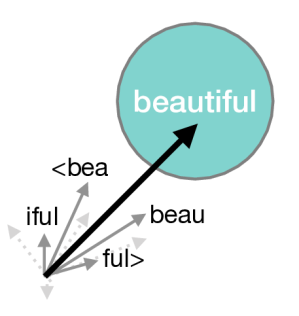
(a)

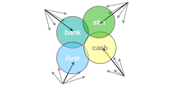
(b)

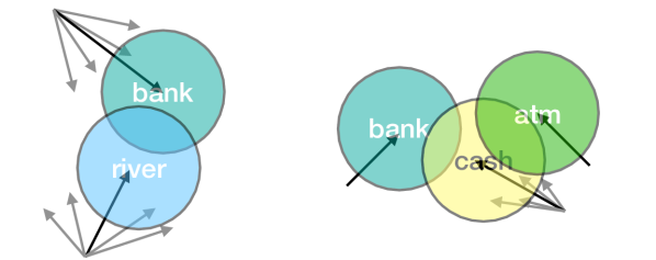
(c)

Figure 1: (1) a Gaussian component and its subword structure. The bold arrow represents the final mean vector, estimated from averaging the grey n-gram vectors. (1) pft-g model: Each Gaussian component’s mean vector is a subword vector. (1) pft-gm model: For each Gaussian mixture distribution, one component’s mean vector is estimated by a subword structure whereas other components are dictionary-based vectors.

3.1 Probabilistic Subword Representation

We represent each word with a Gaussian mixture with $K$ Gaussian components. That is, a word $w$ is associated with a density function $f(x)=\sum_{i=1}^{K}p_{w,i}\mathcal{N}(x;\vec{\mu}_{w,i},\Sigma_{w,i})$ where $\{\mu_{w,i}\}_{k=1}^{K}$ are the mean vectors and $\{\Sigma_{w,i}\}$ are the covariance matrices, and $\{p_{w,i}\}_{k=1}^{K}$ are the component probabilities which sum to $1$.

The mean vectors of Gaussian components hold much of the semantic information in density embeddings. While these models are successful based on word similarity and entailment benchmarks (Vilnis and McCallum, 2014; Athiwaratkun and Wilson, 2017), the mean vectors are often dictionary-level, which can lead to poor semantic estimates for rare words, or the inability to handle words outside the training corpus. We propose using subword structures to estimate the mean vectors. We outline the formulation below.

For word $w$, we estimate the mean vector $\mu_{w}$ with the average over n-gram vectors and its dictionary-level vector. That is,

$$\mu_{w}=\frac{1}{|NG_{w}|+1}\left(v_{w}+\sum_{g\in NG_{w}}z_{g}\right)$$ (1)

where $z_{g}$ is a vector associated with an n-gram $g$, $v_{w}$ is the dictionary representation of word $w$, and $NG_{w}$ is a set of $n$-grams of word $w$. Examples of 3,4-grams for a word “beautiful”, including the beginning-of-word character ‘$\langle$’ and end-of-word character ‘$\rangle$’, are:

• 3-grams: $\langle$be, bea, eau, aut, uti, tif, ful, ul$\rangle$

• 4-grams: $\langle$bea, beau .., iful ,ful$\rangle$

This structure is similar to that of FastText (Bojanowski et al., 2016); however, we note that FastText uses single-prototype deterministic embeddings as well as a training approach that maximizes the negative log-likelihood, whereas we use a multi-prototype probabilistic embedding and for training we maximize the similarity between the words’ probability densities, as described in Sections 3.2 and 3.3

Figure 1 depicts the subword structure for the mean vector. Figure 1 and 1 depict our models, Gaussian probabilistic FastText (pft-g) and Gaussian mixture probabilistic FastText (pft-gm). In the Gaussian case, we represent each mean vector with a subword estimation. For the Gaussian mixture case, we represent one Gaussian component’s mean vector with the subword structure whereas other components’ mean vectors are dictionary-based. This model choice to use dictionary-based mean vectors for other components is to reduce to constraint imposed by the subword structure and promote independence for meaning discovery.

3.2 Similarity Measure between Words

Traditionally, if words are represented by vectors, a common similarity metric is a dot product. In the case where words are represented by distribution functions, we use the generalized dot product in Hilbert space $\langle\cdot,\cdot\rangle_{L_{2}}$, which is called the expected likelihood kernel (Jebara et al., 2004). We define the energy $E(f,g)$ between two words $f$ and $g$ to be $E(f,g)=\log\langle f,g\rangle_{L_{2}}=\log\int f(x)g(x)\ dx$. With Gaussian mixtures $f(x)=\sum_{i=1}^{K}p_{i}\mathcal{N}(x;\vec{\mu}_{f,i},\Sigma_{f,i})$ and $g(x)=\sum_{i=1}^{K}q_{i}\mathcal{N}(x;\vec{\mu}_{g,i},\Sigma_{g,i})$, $\sum_{i=1}^{K}p_{i}=1$, and $\sum_{i=1}^{K}q_{i}=1$, the energy has a closed form:

$$E(f,g)=\log\sum_{j=1}^{K}\sum_{i=1}^{K}p_{i}q_{j}e^{\xi_{i,j}}$$ (2)

where $\xi_{j,j}$ is the partial energy which corresponds to the similarity between component $i$ of the first word $f$ and component $j$ of the second word $g$.

$$\xi_{i,j} \equiv\log\mathcal{N}(0;\vec{\mu}_{f,i}-\vec{\mu}_{g,j},\Sigma_{f,i}+\Sigma_{g,j})$$

$$=-\frac{1}{2}\log\det(\Sigma_{f,i}+\Sigma_{g,j})-\frac{D}{2}\log(2\pi)$$

$$-\frac{1}{2} (\vec{\mu}_{f,i}-\vec{\mu}_{g,j})^{\top}(\Sigma_{f,i}+\Sigma_{g,j})^{-1}(\vec{\mu}_{f,i}-\vec{\mu}_{g,j})$$ (3)

Figure 2 demonstrates the partial energies among the Gaussian components of two words.

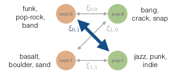
Figure 2: The interactions among Gaussian components of word rock and word pop. The partial energy is the highest for the pair rock:0 (the zeroth component of rock) and pop:1 (the first component of pop), reflecting the similarity in meanings.

3.3 Loss Function

The model parameters that we seek to learn are $v_{w}$ for each word $w$ and $z_{g}$ for each n-gram $g$. We train the model by pushing the energy of a true context pair $w$ and $c$ to be higher than the negative context pair $w$ and $n$ by a margin $m$. We use Adagrad (Duchi et al., 2011) to minimize the following loss to achieve this outcome:

$$L(f,g)=\max\left[0,m-E(f,g)+E(f,n)\right].$$ (4)

We describe how to sample words as well as its positive and negative contexts in Section 3.5.

This loss function together with the Gaussian mixture model with $K>1$ has the ability to extract multiple senses of words. That is, for a word with multiple meanings, we can observe each mode to represent a distinct meaning. For instance, one density mode of “star” is close to the densities of “celebrity” and “hollywood” whereas another mode of “star” is near the densities of “constellation” and “galaxy”.

3.4 Energy Simplification

In theory, it can be beneficial to have covariance matrices as learnable parameters. In practice, Athiwaratkun and Wilson (2017) observe that spherical covariances often perform on par with diagonal covariances with much less computational resources. Using spherical covariances for each component, we can further simplify the energy function as follows:

$$\xi_{i,j}=-\frac{\alpha}{2}\cdot||\mu_{f,i}-\mu_{g,j}||^{2}\,,$$ (5)

where the hyperparameter $\alpha$ is the scale of the inverse covariance term in Equation 3. We note that Equation 5 is equivalent to Equation 3 up to an additive constant given that the covariance matrices are spherical and the same for all components.

3.5 Word Sampling

To generate a context word $c$ of a given word $w$, we pick a nearby word within a context window of a fixed length $\ell$. We also use a word sampling technique similar to Mikolov et al. (2013b). This subsampling procedure selects words for training with lower probabilities if they appear frequently. This technique has an effect of reducing the importance of words such as ‘the’, ‘a’, ‘to’ which can be predominant in a text corpus but are not as meaningful as other less frequent words such as ‘city’, ‘capital’, ‘animal’, etc. In particular, word $w$ has probability $P(w)=1-\sqrt{t/f(w)}$ where $f(w)$ is the frequency of word $w$ in the corpus and $t$ is the frequency threshold.

A negative context word is selected using a distribution $P_{n}(w)\propto U(w)^{3/4}$ where $U(w)$ is a unigram probability of word $w$. The exponent $3/4$ also diminishes the importance of frequent words and shifts the training focus to other less frequent words.

4 Experiments

We have proposed a probabilistic FastText model which combines the flexibility of subword structure with the density embedding approach. In this section, we show that our probabilistic representation with subword mean vectors with the simplified energy function outperforms many word similarity baselines and provides disentangled meanings for polysemies.

First, we describe the training details in Section 4.1. We provide qualitative evaluation in Section 4.2, showing meaningful nearest neighbors for the Gaussian embeddings, as well as the ability to capture multiple meanings by Gaussian mixtures. Our quantitative evaluation in Section 4.3 demonstrates strong performance against the baseline models FastText (Bojanowski et al., 2016) and the dictionary-level Gaussian (w2g) (Vilnis and McCallum, 2014) and Gaussian mixture embeddings (Athiwaratkun and Wilson, 2017) (w2gm). We train our models on foreign language corpuses and show competitive results on foreign word similarity benchmarks in Section 4.4. Finally, we explain the importance of the n-gram structures for semantic sharing in Section 4.5.

4.1 Training Details

We train our models on both English and foreign language datasets. For English, we use the concatenation of ukWac and WackyPedia (Baroni et al., 2009) which consists of $3.376$ billion words. We filter out word types that occur fewer than $5$ times which results in a vocabulary size of 2,677,466.

For foreign languages, we demonstrate the training of our model on French, German, and Italian text corpuses. We note that our model should be applicable for other languages as well. We use FrWac (French), DeWac (German), ItWac (Italian) datasets (Baroni et al., 2009) for text corpuses, consisting of $1.634$, $1.716$ and $1.955$ billion words respectively. We use the same threshold, filtering out words that occur less than $5$ times in each corpus. We have dictionary sizes of $1.3$, $2.7$, and $1.4$ million words for FrWac, DeWac, and ItWac.

We adjust the hyperparameters on the English corpus and use them for foreign languages. Note that the adjustable parameters for our models are the loss margin $m$ in Equation 4 and the scale $\alpha$ in Equation 5. We search for the optimal hyperparameters in a grid $m\in\{0.01,0.1,1,10,100\}$ and $\alpha\in\{\frac{1}{5\times 10^{-3}},\frac{1}{10^{-3}},\frac{1}{2\times 10^{-4}},\frac{1}{1\times 10^{-4}}\}$ on our English corpus. The hyperpameter $\alpha$ affects the scale of the loss function; therefore, we adjust the learning rate appropriately for each $\alpha$. In particular, the learning rates used are $\gamma=\{10^{-4},10^{-5},10^{-6}\}$ for the respective $\alpha$ values.

Other fixed hyperparameters include the number of Gaussian components $K=2$, the context window length $\ell=10$ and the subsampling threshold $t=10^{-5}$. Similar to the setup in FastText, we use n-grams where $n=3,4,5,6$ to estimate the mean vectors.

4.2 Qualitative Evaluation - Nearest neighbors

We show that our embeddings learn the word semantics well by demonstrating meaningful nearest neighbors. Table 1 shows examples of polysemous words such as rock, star, and cell.

Word	Co.	Nearest Neighbors
rock	0	rock:0, rocks:0, rocky:0, mudrock:0, rockscape:0, boulders:0 , coutcrops:0,
rock	1	rock:1, punk:0, punk-rock:0, indie:0, pop-rock:0, pop-punk:0, indie-rock:0, band:1
bank	0	bank:0, banks:0, banker:0, bankers:0, bankcard:0, Citibank:0, debits:0
bank	1	bank:1, banks:1, river:0, riverbank:0, embanking:0, banks:0, confluence:1
star	0	stars:0, stellar:0, nebula:0, starspot:0, stars.:0, stellas:0, constellation:1
star	1	star:1, stars:1, star-star:0, 5-stars:0, movie-star:0, mega-star:0, super-star:0
cell	0	cell:0, cellular:0, acellular:0, lymphocytes:0, T-cells:0, cytes:0, leukocytes:0
cell	1	cell:1, cells:1, cellular:0, cellular-phone:0, cellphone:0, transcellular:0
left	0	left:0, right:1, left-hand:0, right-left:0, left-right-left:0, right-hand:0, leftwards:0
left	1	left:1, leaving:0, leavings:0, remained:0, leave:1, enmained:0, leaving-age:0, sadly-departed:0

Word	Nearest Neighbors
rock	rock, rock-y, rockn, rock-, rock-funk, rock/, lava-rock, nu-rock, rock-pop, rock/ice, coral-rock
bank	bank-, bank/, bank-account, bank., banky, bank-to-bank, banking, Bank, bank/cash, banks.**
star	movie-stars, star-planet, G-star, star-dust, big-star, starsailor, 31-star, star-lit, Star, starsign, pop-stars
cell	cellular, tumour-cell, in-cell, cell/tumour, 11-cell, T-cell, sperm-cell, 2-cells, Cell-to-cell
left	left, left/joined, leaving, left,right, right, left)and, leftsided, lefted, leftside

Table 1: Nearest neighbors of pft-gm (top) and pft-g (bottom). The notation w:i denotes the $i^{th}$ mixture component of the word w.

Table 1 shows the nearest neighbors of polysemous words. We note that subword embeddings prefer words with overlapping characters as nearest neighbors. For instance, “rock-y”, “rockn”, and “rock” are both close to the word “rock”. For the purpose of demonstration, we only show words with meaningful variations and omit words with small character-based variations previously mentioned. However, all words shown are in the top-100 nearest words.

We observe the separation in meanings for the multi-component case; for instance, one component of the word “bank” corresponds to a financial bank whereas the other component corresponds to a river bank. The single-component case also has interesting behavior. We observe that the subword embeddings of polysemous words can represent both meanings. For instance, both “lava-rock” and “rock-pop” are among the closest words to “rock”.

4.3 Word Similarity Evaluation

d	50				300
	w2g	w2gm	pft-g	pft-gm	FastText	w2g	w2gm	pft-g	pft-gm
SL-999	29.35	29.31	27.34	34.13	38.03	38.84	39.62	35.85	39.60
WS-353	71.53	73.47	67.17	71.10	73.88	78.25	79.38	73.75	76.11
MEN-3k	72.58	73.55	70.61	73.90	76.37	78.40	78.76	77.78	79.65
MC-30	76.48	79.08	73.54	79.75	81.20	82.42	84.58	81.90	80.93
RG-65	73.30	74.51	70.43	78.19	79.98	80.34	80.95	77.57	79.81
YP-130	41.96	45.07	37.10	40.91	53.33	46.40	47.12	48.52	54.93
MT-287	64.79	66.60	63.96	67.65	67.93	67.74	69.65	66.41	69.44
MT-771	60.86	60.82	60.40	63.86	66.89	70.10	70.36	67.18	69.68
RW-2k	28.78	28.62	44.05	42.78	48.09	35.49	42.73	50.37	49.36
avg.	42.32	42.76	44.35	46.47	49.28	47.71	49.54	49.86	51.10

Table 2: Spearman’s Correlation $\rho\times 100$ on Word Similarity Datasets.

We evaluate our embeddings on several standard word similarity datasets, namely, SL-999 (Hill et al., 2014), WS-353 (Finkelstein et al., 2002), MEN-3k (Bruni et al., 2014), MC-30 (Miller and Charles, 1991), RG-65 (Rubenstein and Goodenough, 1965), YP-130 (Yang and Powers, 2006), MTurk(-287,-771) (Radinsky et al., 2011; Halawi et al., 2012), and RW-2k (Luong et al., 2013). Each dataset contains a list of word pairs with a human score of how related or similar the two words are. We use the notation dataset-num to denote the number of word pairs num in each evaluation set. We note that the dataset RW focuses more on infrequent words and SimLex-999 focuses on the similarity of words rather than relatedness. We also compare pft-gm with other multi-prototype embeddings in the literature using SCWS (Huang et al., 2012), a word similarity dataset that is aimed to measure the ability of embeddings to discern multiple meanings.

We calculate the Spearman correlation (Spearman, 1904) between the labels and our scores generated by the embeddings. The Spearman correlation is a rank-based correlation measure that assesses how well the scores describe the true labels. The scores we use are cosine-similarity scores between the mean vectors. In the case of Gaussian mixtures, we use the pairwise maximum score:

$$s(f,g)=\max_{i\in 1,\ldots,K}\max_{j\in 1,\ldots,K}\frac{\mu_{f,i}\cdot\mu_{g,j}}{||\mu_{f,i}||\cdot||\mu_{g,j}||}.$$ (6)

The pair $(i,j)$ that achieves the maximum cosine similarity corresponds to the Gaussian component pair that is the closest in meanings. Therefore, this similarity score yields the most related senses of a given word pair. This score reduces to a cosine similarity in the Gaussian case $(K=1)$.

4.3.1 Comparison Against Dictionary-Level Density Embeddings and FastText

We compare our models against the dictionary-level Gaussian and Gaussian mixture embeddings in Table 2, with $50$-dimensional and $300$-dimensional mean vectors. The 50-dimensional results for w2g and w2gm are obtained directly from Athiwaratkun and Wilson (2017). For comparison, we use the public code to train the 300-dimensional w2g and w2gm models and the publicly available FastText model.

We calculate Spearman’s correlations for each of the word similarity datasets. These datasets vary greatly in the number of word pairs; therefore, we mark each dataset with its size for visibility. For a fair and objective comparison, we calculate a weighted average of the correlation scores for each model.

Our pft-gm achieves the highest average score among all competing models, outperforming both FastText and the dictionary-level embeddings w2g and w2gm. Our unimodal model pft-g also outperforms the dictionary-level counterpart w2g and FastText. We note that the model w2gm appears quite strong according to Table 2, beating pft-gm on many word similarity datasets. However, the datasets that w2gm performs better than pft-gm often have small sizes such as MC-30 or RG-65, where the Spearman’s correlations are more subject to noise. Overall, pft-gm outperforms w2gm by $3.1\%$ and $8.7\%$ in $300$ and $50$ dimensional models. In addition, pft-g and pft-gm also outperform FastText by $1.2\%$ and $3.7\%$ respectively.

4.3.2 Comparison Against Multi-Prototype Models

In Table 3, we compare $50$ and $300$ dimensional pft-gm models against the multi-prototype embeddings described in Section 2 and the existing multimodal density embeddings w2gm. We use the word similarity dataset SCWS (Huang et al., 2012) which contains words with potentially many meanings, and is a benchmark for distinguishing senses. We use the maximum similarity score (Equation 6), denoted as MaxSim. AveSim denotes the average of the similarity scores, rather than the maximum.

We outperform the dictionary-based density embeddings w2gm in both $50$ and $300$ dimensions, demonstrating the benefits of subword information. Our model achieves state-of-the-art results, similar to that of Neelakantan et al. (2014).

Model	Dim	$\rho\times 100$
Huang AvgSim	50	62.8
Tian MaxSim	50	63.6
w2gm MaxSim	50	62.7
Neelakantan AvgSim	50	64.2
pft-gm MaxSim	50	63.7
Chen-M AvgSim	200	66.2
w2gm MaxSim	200	65.5
Neelakantan AvgSim	300	67.2
w2gm MaxSim	300	66.5
pft-gm MaxSim	300	67.2

Table 3: Spearman’s Correlation $\rho\times 100$ on word similarity dataset SCWS.

Lang.	Evaluation	FastText	w2g	w2gm	pft-g	pft-gm
fr	WS353	38.2	16.73	20.09	41.0	41.3
de	GUR350	70	65.01	69.26	77.6	78.2
	GUR65	81	74.94	76.89	81.8	85.2
it	WS353	57.1	56.02	61.09	60.2	62.5
	SL-999	29.3	29.44	34.91	29.3	33.7

Table 4: Word similarity evaluation on foreign languages.

4.4 Evaluation on Foreign Language Embeddings

We evaluate the foreign-language embeddings on word similarity datasets in respective languages. We use Italian WordSim353 and Italian SimLex-999 (Leviant and Reichart, 2015) for Italian models, GUR350 and GUR65 (Gurevych, 2005) for German models, and French WordSim353 (Finkelstein et al., 2002) for French models. For datasets GUR350 and GUR65, we use the results reported in the FastText publication (Bojanowski et al., 2016). For other datasets, we train FastText models for comparison using the public code on our text corpuses. We also train dictionary-level models w2g, and w2gm for comparison.

Table 4 shows the Spearman’s correlation results of our models. We outperform FastText on many word similarity benchmarks. Our results are also significantly better than the dictionary-based models, w2g and w2gm. We hypothesize that w2g and w2gm can perform better than the current reported results given proper pre-processing of words due to special characters such as accents.

We investigate the nearest neighbors of polysemies in foreign languages and also observe clear sense separation. For example, piano in Italian can mean “floor” or “slow”. These two meanings are reflected in the nearest neighbors where one component is close to piano-piano, pianod which mean “slowly” whereas the other component is close to piani (floors), istrutturazione (renovation) or infrastruttre (infrastructure). Table 5 shows additional results, demonstrating that the disentangled semantics can be observed in multiple languages.

Word	Meaning	Nearest Neighbors
(it) secondo	2nd	Secondo (2nd), terzo (3rd) , quinto (5th), primo (first), quarto (4th), ultimo (last)
(it) secondo	according to	conformit (compliance), attenendosi (following), cui (which), conformemente (accordance with)
(it) porta	lead, bring	portano (lead), conduce (leads), portano, porter, portando (bring), costringe (forces)
(it) porta	door	porte (doors), finestrella (window), finestra (window), portone (doorway), serratura (door lock)
(fr) voile	veil	voiles (veil), voiler (veil), voilent (veil), voilement, foulard (scarf), voils (veils), voilant (veiling)
(fr) voile	sail	catamaran (catamaran), driveur (driver), nautiques (water), Voile (sail), driveurs (drivers)
(fr) temps	weather	brouillard (fog), orageuses (stormy), nuageux (cloudy)
(fr) temps	time	mi-temps (half-time), partiel (partial), Temps (time), annualis (annualized), horaires (schedule)
(fr) voler	steal	envoler (fly), voleuse (thief), cambrioler (burgle), voleur (thief), violer (violate), picoler (tipple)
(fr) voler	fly	airs (air), vol (flight), volent (fly), envoler (flying), atterrir (land)

Table 5: Nearest neighbors of polysemies based on our foreign language pft-gm models.

4.5 Qualitative Evaluation - Subword Decomposition

One of the motivations for using subword information is the ability to handle out-of-vocabulary words. Another benefit is the ability to help improve the semantics of rare words via subword sharing. Due to an observation that text corpuses follow Zipf’s power law (Zipf, 1949), words at the tail of the occurrence distribution appears much less frequently. Training these words to have a good semantic representation is challenging if done at the word level alone. However, an n-gram such as ‘abnorm’ is trained during both occurrences of “abnormal” and “abnormality” in the corpus, hence further augments both words’s semantics.

Figure 3 shows the contribution of n-grams to the final representation. We filter out to show only the n-grams with the top-5 and bottom-5 similarity scores. We observe that the final representations of both words align with n-grams “abno”, “bnor”, “abnorm”, “anbnor”, “$\textless$abn”. In fact, both “abnormal” and “abnormality” share the same top-5 n-grams. Due to the fact that many rare words such as “autobiographer”, “circumnavigations”, or “hypersensitivity” are composed from many common sub-words, the n-gram structure can help improve the representation quality.

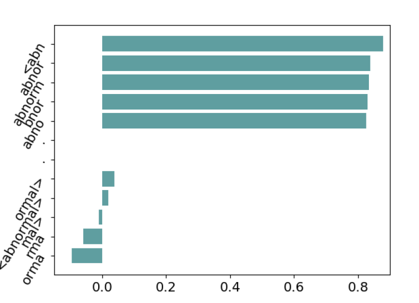
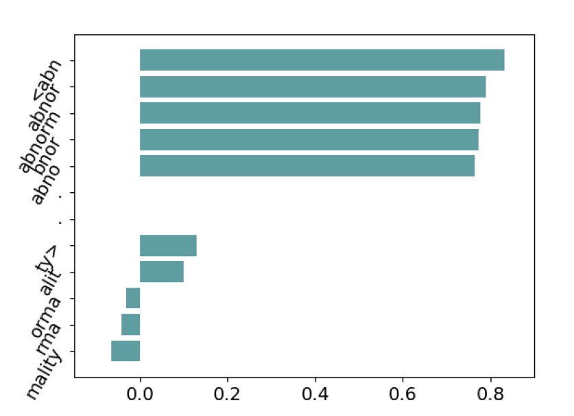
Figure 3: Contribution of each n-gram vector to the final representation for word “abnormal” (top) and “abnormality” (bottom). The x-axis is the cosine similarity between each n-gram vector $z_{g}^{(w)}$ and the final vector $\mu_{w}$.

5 Numbers of Components

It is possible to train our approach with $K>2$ mixture components; however, Athiwaratkun and Wilson (2017) observe that dictionary-level Gaussian mixtures with $K=3$ do not overall improve word similarity results, even though these mixtures can discover $3$ distinct senses for certain words. Indeed, while $K>2$ in principle allows for greater flexibility than $K=2$, most words can be very flexibly modelled with a mixture of two Gaussians, leading to $K=2$ representing a good balance between flexibility and Occam’s razor.

Even for words with single meanings, our pft model with $K=2$ often learns richer representations than a $K=1$ model. For example, the two mixture components can learn to cluster together to form a more heavy tailed unimodal distribution which captures a word with one dominant meaning but with close relationships to a wide range of other words.

In addition, we observe that our model with $K$ components can capture more than $K$ meanings. For instance, in $K=1$ model, the word pairs (“cell”, “jail”) and (“cell”, “biology”) and (“cell”, “phone”) will all have positive similarity scores based on $K=1$ model. In general, if a word has multiple meanings, these meanings are usually compressed into the linear substructure of the embeddings (Arora et al., 2016). However, the pairs of non-dominant words often have lower similarity scores, which might not accurately reflect their true similarities.

6 Conclusion and Future Work

We have proposed models for probabilistic word representations equipped with flexible sub-word structures, suitable for rare and out-of-vocabulary words. The proposed probabilistic formulation incorporates uncertainty information and naturally allows one to uncover multiple meanings with multimodal density representations. Our models offer better semantic quality, outperforming competing models on word similarity benchmarks. Moreover, our multimodal density models can provide interpretable and disentangled representations, and are the first multi-prototype embeddings that can handle rare words.

Future work includes an investigation into the trade-off between learning full covariance matrices for each word distribution, computational complexity, and performance. This direction can potentially have a great impact on tasks where the variance information is crucial, such as for hierarchical modeling with probability distributions (Athiwaratkun and Wilson, 2018).

Other future work involves co-training pft on many languages. Currently, existing work on multi-lingual embeddings align the word semantics on pre-trained vectors (Smith et al., 2017), which can be suboptimal due to polysemies. We envision that the multi-prototype nature can help disambiguate words with multiple meanings and facilitate semantic alignment.

References

- Arora et al. (2016) Sanjeev Arora, Yuanzhi Li, Yingyu Liang, Tengyu Ma, and Andrej Risteski. 2016. Linear algebraic structure of word senses, with applications to polysemy. CoRR abs/1601.03764. http://arxiv.org/abs/1601.03764.
- Athiwaratkun and Wilson (2017) Ben Athiwaratkun and Andrew Gordon Wilson. 2017. Multimodal word distributions. In ACL. https://arxiv.org/abs/1704.08424.
- Athiwaratkun and Wilson (2018) Ben Athiwaratkun and Andrew Gordon Wilson. 2018. On modeling hierarchical data via probabilistic order embeddings. ICLR .
- Baroni et al. (2009) Marco Baroni, Silvia Bernardini, Adriano Ferraresi, and Eros Zanchetta. 2009. The wacky wide web: a collection of very large linguistically processed web-crawled corpora. Language Resources and Evaluation 43(3):209–226. https://doi.org/10.1007/s10579-009-9081-4.
- Bengio et al. (2003) Yoshua Bengio, Réjean Ducharme, Pascal Vincent, and Christian Janvin. 2003. A neural probabilistic language model. Journal of Machine Learning Research 3:1137–1155. http://www.jmlr.org/papers/v3/bengio03a.html.
- Bojanowski et al. (2016) Piotr Bojanowski, Edouard Grave, Armand Joulin, and Tomas Mikolov. 2016. Enriching word vectors with subword information. CoRR abs/1607.04606. http://arxiv.org/abs/1607.04606.
- Bruni et al. (2014) Elia Bruni, Nam Khanh Tran, and Marco Baroni. 2014. Multimodal distributional semantics. J. Artif. Int. Res. 49(1):1–47. http://dl.acm.org/citation.cfm?id=2655713.2655714.
- Chen et al. (2014) Xinxiong Chen, Zhiyuan Liu, and Maosong Sun. 2014. A unified model for word sense representation and disambiguation. In Proceedings of the 2014 Conference on Empirical Methods in Natural Language Processing, EMNLP 2014, October 25-29, 2014, Doha, Qatar, A meeting of SIGDAT, a Special Interest Group of the ACL. pages 1025–1035. http://aclweb.org/anthology/D/D14/D14-1110.pdf.
- Collobert and Weston (2008) Ronan Collobert and Jason Weston. 2008. A unified architecture for natural language processing: deep neural networks with multitask learning. In Machine Learning, Proceedings of the Twenty-Fifth International Conference (ICML 2008), Helsinki, Finland, June 5-9, 2008. pages 160–167. http://doi.acm.org/10.1145/1390156.1390177.
- Duchi et al. (2011) John C. Duchi, Elad Hazan, and Yoram Singer. 2011. Adaptive subgradient methods for online learning and stochastic optimization. Journal of Machine Learning Research 12:2121–2159. http://dl.acm.org/citation.cfm?id=2021068.
- Finkelstein et al. (2002) Lev Finkelstein, Evgeniy Gabrilovich, Yossi Matias, Ehud Rivlin, Zach Solan, Gadi Wolfman, and Eytan Ruppin. 2002. Placing search in context: the concept revisited. ACM Trans. Inf. Syst. 20(1):116–131. http://doi.acm.org/10.1145/503104.503110.
- Gurevych (2005) Iryna Gurevych. 2005. Using the structure of a conceptual network in computing semantic relatedness. In Natural Language Processing - IJCNLP 2005, Second International Joint Conference, Jeju Island, Korea, October 11-13, 2005, Proceedings. pages 767–778.
- Halawi et al. (2012) Guy Halawi, Gideon Dror, Evgeniy Gabrilovich, and Yehuda Koren. 2012. Large-scale learning of word relatedness with constraints. In The 18th ACM SIGKDD International Conference on Knowledge Discovery and Data Mining, KDD ’12, Beijing, China, August 12-16, 2012. pages 1406–1414. http://doi.acm.org/10.1145/2339530.2339751.
- Hill et al. (2014) Felix Hill, Roi Reichart, and Anna Korhonen. 2014. Simlex-999: Evaluating semantic models with (genuine) similarity estimation. CoRR abs/1408.3456. http://arxiv.org/abs/1408.3456.
- Huang et al. (2012) Eric H. Huang, Richard Socher, Christopher D. Manning, and Andrew Y. Ng. 2012. Improving word representations via global context and multiple word prototypes. In The 50th Annual Meeting of the Association for Computational Linguistics, Proceedings of the Conference, July 8-14, 2012, Jeju Island, Korea - Volume 1: Long Papers. pages 873–882. http://www.aclweb.org/anthology/P12-1092.
- Jebara et al. (2004) Tony Jebara, Risi Kondor, and Andrew Howard. 2004. Probability product kernels. Journal of Machine Learning Research 5:819–844.
- Kim et al. (2016) Yoon Kim, Yacine Jernite, David Sontag, and Alexander M. Rush. 2016. Character-aware neural language models. In Proceedings of the Thirtieth AAAI Conference on Artificial Intelligence, February 12-17, 2016, Phoenix, Arizona, USA.. pages 2741–2749.
- Kuru et al. (2016) Onur Kuru, Ozan Arkan Can, and Deniz Yuret. 2016. Charner: Character-level named entity recognition. In COLING 2016, 26th International Conference on Computational Linguistics, Proceedings of the Conference: Technical Papers, December 11-16, 2016, Osaka, Japan. pages 911–921. http://aclweb.org/anthology/C/C16/C16-1087.pdf.
- Lee et al. (2017) Jason Lee, Kyunghyun Cho, and Thomas Hofmann. 2017. Fully character-level neural machine translation without explicit segmentation. TACL 5:365–378. https://transacl.org/ojs/index.php/tacl/article/view/1051.
- Leviant and Reichart (2015) Ira Leviant and Roi Reichart. 2015. Judgment language matters: Multilingual vector space models for judgment language aware lexical semantics. CoRR abs/1508.00106. http://arxiv.org/abs/1508.00106.
- Luong et al. (2013) Minh-Thang Luong, Richard Socher, and Christopher D. Manning. 2013. Better word representations with recursive neural networks for morphology. In CoNLL. Sofia, Bulgaria.
- Mikolov et al. (2013a) Tomas Mikolov, Kai Chen, Greg Corrado, and Jeffrey Dean. 2013a. Efficient estimation of word representations in vector space. CoRR abs/1301.3781. http://arxiv.org/abs/1301.3781.
- Mikolov et al. (2013b) Tomas Mikolov, Kai Chen, Greg Corrado, and Jeffrey Dean. 2013b. Efficient estimation of word representations in vector space. CoRR abs/1301.3781. http://arxiv.org/abs/1301.3781.
- Mikolov et al. (2011) Tomas Mikolov, Stefan Kombrink, Lukás Burget, Jan Cernocký, and Sanjeev Khudanpur. 2011. Extensions of recurrent neural network language model. In Proceedings of the IEEE International Conference on Acoustics, Speech, and Signal Processing, ICASSP 2011, May 22-27, 2011, Prague Congress Center, Prague, Czech Republic. pages 5528–5531. https://doi.org/10.1109/ICASSP.2011.5947611.
- Miller and Charles (1991) George A. Miller and Walter G. Charles. 1991. Contextual Correlates of Semantic Similarity. Language & Cognitive Processes 6(1):1–28. https://doi.org/10.1080/01690969108406936.
- Neelakantan et al. (2014) Arvind Neelakantan, Jeevan Shankar, Alexandre Passos, and Andrew McCallum. 2014. Efficient non-parametric estimation of multiple embeddings per word in vector space. In Proceedings of the 2014 Conference on Empirical Methods in Natural Language Processing, EMNLP 2014, October 25-29, 2014, Doha, Qatar, A meeting of SIGDAT, a Special Interest Group of the ACL. pages 1059–1069. http://aclweb.org/anthology/D/D14/D14-1113.pdf.
- Pennington et al. (2014) Jeffrey Pennington, Richard Socher, and Christopher D. Manning. 2014. Glove: Global vectors for word representation. In Proceedings of the 2014 Conference on Empirical Methods in Natural Language Processing, EMNLP 2014, October 25-29, 2014, Doha, Qatar, A meeting of SIGDAT, a Special Interest Group of the ACL. pages 1532–1543. http://aclweb.org/anthology/D/D14/D14-1162.pdf.
- Radinsky et al. (2011) Kira Radinsky, Eugene Agichtein, Evgeniy Gabrilovich, and Shaul Markovitch. 2011. A word at a time: Computing word relatedness using temporal semantic analysis. In Proceedings of the 20th International Conference on World Wide Web. WWW ’11, pages 337–346. http://doi.acm.org/10.1145/1963405.1963455.
- Rubenstein and Goodenough (1965) Herbert Rubenstein and John B. Goodenough. 1965. Contextual correlates of synonymy. Commun. ACM 8(10):627–633. http://doi.acm.org/10.1145/365628.365657.
- Smith et al. (2017) Samuel L. Smith, David H. P. Turban, Steven Hamblin, and Nils Y. Hammerla. 2017. Offline bilingual word vectors, orthogonal transformations and the inverted softmax. CoRR abs/1702.03859. http://arxiv.org/abs/1702.03859.
- Spearman (1904) C. Spearman. 1904. The proof and measurement of association between two things. American Journal of Psychology 15:88–103.
- Tian et al. (2014) Fei Tian, Hanjun Dai, Jiang Bian, Bin Gao, Rui Zhang, Enhong Chen, and Tie-Yan Liu. 2014. A probabilistic model for learning multi-prototype word embeddings. In COLING 2014, 25th International Conference on Computational Linguistics, Proceedings of the Conference: Technical Papers, August 23-29, 2014, Dublin, Ireland. pages 151–160. http://aclweb.org/anthology/C/C14/C14-1016.pdf.
- Vilnis and McCallum (2014) Luke Vilnis and Andrew McCallum. 2014. Word representations via gaussian embedding. CoRR abs/1412.6623. http://arxiv.org/abs/1412.6623.
- Yang and Powers (2006) Dongqiang Yang and David M. W. Powers. 2006. Verb similarity on the taxonomy of wordnet. In In the 3rd International WordNet Conference (GWC-06), Jeju Island, Korea.
- Zhao and Zhang (2016) Shenjian Zhao and Zhihua Zhang. 2016. An efficient character-level neural machine translation. CoRR abs/1608.04738. http://arxiv.org/abs/1608.04738.
- Zipf (1949) G.K. Zipf. 1949. Human behavior and the principle of least effort: an introduction to human ecology. Addison-Wesley Press. https://books.google.com/books?id=1tx9AAAAIAAJ.