Integral identities for reflection, transmission and scattering coefficients

Abstract

Several integral identities related to acoustic scattering are presented. In each case the identity involves the integral over frequency of a physical quantity. For instance, the integrated transmission loss, a measure of the transmitted acoustic energy through an inhomogeneous layer, is shown to have a simple expression in terms of spatially averaged physical quantities. Known identities for the extinction cross section and for the acoustic energy loss in a slab with a rigid backing, are shown to be special cases of a general procedure for finding such integral identities.

I Introduction

Identities for scattering coefficients that involve integrals over all frequencies, or equivalently over all wavelengths, provide a useful means to characterize scattering independent of frequency using a single parameter. However, there are very few such identities available. An important example is the integral of the extinction (which is the sum of the rate of energy absorption and the scattering cross-section) over all wavelengths Purcell69 . The integrated extinction (IE) is a natural metric for quantifying scattering reduction Sohl2007 ; Monticone13 . The IE has the important property that it is proportional to a linear combination of the monopole and dipole amplitudes if the scattering is causal Sohl07 ; Norris2015 , that is, the scattered wavefront in the forward direction arrives after an equivalent plane wavefront in the background medium. Causal scattering is the default for electromagnetics, although there is no such limitation for acoustic or elastic waves. Many scattering situations of interest in acoustics are non-causal, such as metal objects in water or air, for which the causal IE expression Purcell69 ; Sohl07 does not apply. However, by considering the scattering in the time domain, it is possible to provide an expression applicable to all types of scatterers. The generalization of Purcell’s result to non-causal scattering can be found in Norris2015 .

The only other integral identity known to the author relates the integral over all wavelengths of the acoustic absorption of a slab with rigid backing to the static effective bulk modulus of the slab Yang2017 ; Yang2017a . This result, based on work by Rozanov Rozanov2000 and on the Bode-Fano theorem Fano1950 , reduces an integral of the logarithm of the absolute value of the acoustic reflection coefficient to a form that can be interpreted in terms of static parameters plus a denumerable set of complex numbers defined by the zeros of the reflection coefficient as a function of frequency.

The purpose of the paper is to present several new integral identities related to acoustic scattering. Some of these identities are similar to the one found previously Yang2017 ; Yang2017a , requiring knowledge of the infinite set of zeros of a reflection coefficient. However, new identities are presented which require only purely static physical parameters, such as the total mass, or the effective compressibility.

We begin in §II by considering some consequences of a signal being causal. The acoustic scattering problem is defined in §III. The main results are given in §IV, including integral identities for the reflection and transmission coefficients in one-dimensional configurations.

II Causal signal results

The real-valued signal is called causal if it is zero before $t=0$,

$$s(t)=0,\ \ t<0.$$ (1)

The Fourier transform of the causal signal,

$$S(\omega)=\int_{0}^{\infty}s(t)e^{\mathrm{i}\omega t}\operatorname{d}t,$$ (2)

is analytic in the upper half plane (or causal half plane) of the complex frequency $\operatorname{Im}\omega>0$. It may have zeros at the discrete set of frequencies $\{\omega_{n}\}$ in the upper half plane. The additional property $S(-\omega^{*})=S^{*}(\omega)$, with ^∗ the complex conjugate, follows from the fact that $s(t)$ is real. The low frequency expansion of the Fourier transform is

$$S(\omega)=S_{0}+\mathrm{i}\omega S_{1}+(\mathrm{i}\omega)^{2}S_{2}+{\cal O}(\omega^{3})$$ (3)

where $S_{j}$, $j=0,1,2,\ldots$ are real valued. The coefficients can be identified from (2) as

$$S_{n}=\frac{1}{n!}\int_{0}^{\infty}s(t)t^{n}\operatorname{d}t.$$ (4)

These integrals are well defined if the function $s(t)$ decays fast enough as $t\to\infty$, which is certainly true if the signal is of finite duration, as is assumed here.

The Fourier transform of a causal function satisfies the Sokhotski-Plemelj relations for real values of $\omega$ (Nuss72, , eq. (1.6.7))

$$S(\omega)=\frac{1}{\mathrm{i}\pi}\mathchoice{{\vbox{\hbox{$\textstyle-$}}\kern-4.86108pt}}{{\vbox{\hbox{$\scriptstyle-$}}\kern-3.25pt}}{{\vbox{\hbox{$\scriptscriptstyle-$}}\kern-2.29166pt}}{{\vbox{\hbox{$\scriptscriptstyle-$}}\kern-1.875pt}}\!\int_{-\infty}^{\infty}\frac{S(\omega^{\prime})\operatorname{d}\omega^{\prime}}{\omega^{\prime}-\omega},$$ (5)

where $\mathchoice{{\vbox{\hbox{$\textstyle-$}}\kern-4.86108pt}}{{\vbox{\hbox{$\scriptstyle-$}}\kern-3.25pt}}{{\vbox{\hbox{$\scriptscriptstyle-$}}\kern-2.29166pt}}{{\vbox{\hbox{$\scriptscriptstyle-$}}\kern-1.875pt}}\!\int$ denotes principal value integral. Equation (5) is equivalent to $S(\omega)=\mathrm{i}\cal{H}(S)(\omega)$ where $\cal{H}(S)$ is the Hilbert transform. The real and imaginary parts of $S(\omega)$ on the real $\omega-$axis are therefore related to one another by the well known identities $\operatorname{Im}S(\omega)=\cal{H}(\operatorname{Re}S)(\omega)$ and $\operatorname{Re}S(\omega)=-\cal{H}(\operatorname{Im}S)(\omega)$. The following identities result from expanding (5) about $\omega=0$ for a real-valued signal, with details available in Appendix A,

$$S_{0} =\frac{2}{\pi}\int_{0}^{\infty}\operatorname{Im}S(\omega)\frac{\operatorname{d}\omega}{\omega},$$ (6a)

$$S_{1} =\frac{2}{\pi}\int_{0}^{\infty}\big{(}S_{0}-\operatorname{Re}S(\omega)\big{)}\frac{\operatorname{d}\omega}{\omega^{2}},$$ (6b)

$$S_{2} =\frac{2}{\pi}\int_{0}^{\infty}\big{(}\omega S_{1}-\operatorname{Im}S(\omega)\big{)}\frac{\operatorname{d}\omega}{\omega^{3}},\ldots.$$ (6c)

In dealing with acoustic transfer functions it is important to distinguish between minimum phase and non-minimum phase functions. The canonical decomposition of a non-minimum phase transfer function is Victor1989

$$S(\omega)=\mathrm{e}^{\mathrm{i}\omega D}S_{\text{mp}}(\omega)\prod_{j}Z(\omega,\omega_{j})$$ (7)

where $S_{\text{mp}}(\omega)$ is the unique minimum phase transfer function,

$$Z(\omega,u)=\frac{\omega-u}{\omega-u^{*}}$$ (8)

and the set of complex frequencies $\{\omega_{j}\}$ are in the causal half plane. The delay $D$ is the largest value for which $s(t-D)$ is causal. The minimum phase transfer function has no zeros in the upper half plane whereas $S(\omega)$ has zeros at $\{\omega_{j}\}$. Note that any zero of the form $\omega_{j}=\alpha_{j}+\mathrm{i}\beta_{j}$, $\omega_{j}\geq 0$, is accompanied by $\omega_{j}^{\prime}=-\alpha_{j}+\mathrm{i}\beta_{j}$. This ensures that $S_{\text{mp}}(-\omega^{*})=S_{\text{mp}}^{*}(\omega)$, and hence the causal time-domain function $s_{\text{mp}}^{*}(t)$ is real-valued.

Since $|S_{\text{mp}}(\omega)|=|S(\omega)|$ for real $\omega$, it follows that the real parts of the two functions $\ln S_{\text{mp}}(\omega)$ and $\ln S(\omega)$ coincide. The imaginary parts of these two functions clearly differ, and most importantly, the real and imaginary parts of the minimum phase function $\ln S_{\text{mp}}(\omega)$ are related by the Hilbert transform relations. This property does not extend to the non-minimum phase function.

Minimum phase identification requires assumptions about the physical system McDaniel99 ; McDaniel2001 . If a transfer function, such as a reflection coefficient, is minimum phase then its phase as a function of frequency is uniquely defined by the amplitude. Conversely, the phase is not uniquely defined by the amplitude if the transfer function is not minimum phase.

We next consider several applications based on the low frequency behavior of minimum phase functions $S(\omega)$ with the common condition $S_{0}=0$. The results all follow from the following identity, which is a consequence of (6b).

Lemma 1

Let $S(\omega)$ be the Fourier transform of a causal real-valued signal with $S(0)=0$. Then

$$\int_{0}^{\infty}\operatorname{Re}S(\omega)\frac{\operatorname{d}\omega}{\omega^{2}}=-\frac{\pi}{2}S_{1}$$ (9)

where

$$S_{1}=-\mathrm{i}\left.\frac{\operatorname{d}S}{\operatorname{d}\omega}\right|_{\omega=0}.$$ (10)

The results in §II are based upon a causal scattering process; that is, the forward scattered signal follows the incoming signal. In the absence of material damping when the wave speed is real, there is no ambiguity in the meaning of causal. With absorption present, the strict definition requires considering how a sharp delta pulse transmits.

III Acoustic scattering

The acoustic pressure $p({\bf x})\in{\mathbb{C}}$ satisfies the Helmholtz equation outside of a finite region $\Omega$, the scatterer,

$$\nabla^{2}p+k^{2}p=0,\ \ {\bf x}\in{\mathbb{R}}^{d}/\Omega.$$ (11)

The system may be one, two or three-dimensional, $d=1,2$ or $3$. Time harmonic dependence is considered with $k=\omega/c$ and $c$ is the sound speed, $c=(C\rho)^{-1/2}$ where the uniform exterior acoustic medium has mass density $\rho$ and compressibility $C$. The factor $e^{-i\omega t}$ is understood and omitted.

The scatterer, $\Omega$, may be an inhomogeneous acoustic or elastic object. The specific results will be limited to acoustic scatterers of density $\rho^{\prime}$ and compressibility $C^{\prime}$. Damping in the scatterer may be included by considering the material properties as frequency dependent complex parameters $\rho^{\prime}({\bf x},\omega)$, $C^{\prime}({\bf x},\omega)$ and derived quantities, the wave speed $c^{\prime}({\bf x},\omega)=(C^{\prime}\rho^{\prime})^{-1/2}$ and impedance $z^{\prime}({\bf x},\omega)=(\rho^{\prime}/C^{\prime})^{1/2}$. The zero frequency limits, or static values, will play an important role in our results, and we therefore denote them

$$\rho_{0}^{\prime} =\rho^{\prime}({\bf x},0),\ \ C_{0}^{\prime}=C^{\prime}({\bf x},0),$$ (12)

$$c_{0}^{\prime} =c^{\prime}({\bf x},0),\ \ z_{0}^{\prime}=z^{\prime}({\bf x},0).$$

Note that these are necessarily real-valued quantities.

The total acoustic pressure $p$ comprises an incident plane wave $e^{\mathrm{i}kx}$ plus the scattered pressure $p_{s}$,

$$p=e^{\mathrm{i}kx}+p_{s}({\bf x}).$$ (13)

The scattering amplitude $F(\theta,\omega)$ is defined by

$$p_{s}=F(\theta,\omega)\,\Big{(}\frac{k}{\mathrm{i}2\pi r}\Big{)}^{\frac{d-1}{2}}\,e^{\mathrm{i}kr}\,\big{[}1+{\cal O}\big{(}\frac{1}{kr}\big{)}\big{]}$$ (14)

as $r=|{\bf x}|\to\infty$, where $\theta$ is the scattering direction, $\theta=0$ corresponding to the direction of incidence $\hat{\bf k}$. Note that (14) is exact in one dimension, in which case $\theta$ only takes the values $0$ and $\pi$, with

$$T(\omega)=1+F(0,\omega),\ \ R(\omega)=F(\pi,\omega)$$ (15)

the transmission and reflection coefficients, respectively.

IV Integral identities

IV.1 Integrated extinction

The extinction cross section is defined as $\sigma=\sigma_{\text{sc}}+\sigma_{\text{ab}}$ with $\sigma_{\text{ab}}$ the absorption cross section (zero in the absence of loss), and $\sigma_{\text{sc}}$ is the scattering cross section

$$\sigma_{\text{sc}}(\omega)=\int|p_{s}|^{2}\operatorname{d}s$$ (16)

where the integral is around any surface enclosing the scatterer. The optical theorem relates the extinction to the forward scattering amplitude,

$$\sigma=-2\,\operatorname{Re}S(\omega)\ \ \text{where}\ S(\omega)\equiv F(0,\omega).$$ (17)

The integrated extinction (IE),

$$\int_{0}^{\infty}\frac{\sigma(\omega)}{\omega^{2}}\,\operatorname{d}\omega\,\geq 0,$$ (18)

defines the total cross section over all frequencies.

It follows from Lemma 1, Eqs. (17), (18) and the fact that the forward scattering amplitude vanishes at zero frequency ($S_{0}=0$) that

$$\int_{0}^{\infty}\frac{\sigma(\omega)}{\omega^{2}}\,\operatorname{d}\omega=\pi S_{1}.$$ (19)

The identity (19) for $d=3$ was derived by Purcell Purcell69 for electromagnetics and was first used in acoustics by Sohl et al. Sohl07 . Equation (19) is, however, restricted to scattering for which the forward scattered impulse function (the time domain version of $S(\omega)$) is strictly causal. This is always the case if the wave speed in the scatterer is everywhere less than that of the exterior medium. However, if the scatterer comprises faster material such that the forward amplitude precedes the direct wave in time, then the function $S(\omega)$ is no longer analytic in the upper half plane, and (19) is not valid. The problem arises from the strict definition of the scattered amplitude in Eq. (14) which allows use of the optical theorem. Resolution of this issue can be found in Norris2015 which describes the generalization of (19) to all possible scatterers. Here we will only consider scattering such that (19) holds.

The zero frequency limit in (19) allows us to interpret $S_{1}$ and hence the IE in terms of quasistatic properties. For instance, if the scatterer has volume $|\Omega|$, compressibility $C^{\prime}({\bf x},\omega)$ and uniform density $\rho^{\prime}(\omega)$, then Sohl07

$$\int_{0}^{\infty}\frac{\sigma(\omega)}{\omega^{2}}\,\operatorname{d}\omega=\frac{\pi}{2c}\Big{(}\big{(}\frac{\langle C_{0}^{\prime}\rangle}{C}-1\big{)}|\Omega|-\hat{\bf k}\cdot{\bm{\gamma}}\Big{(}\frac{\rho}{\rho_{0}^{\prime}}\Big{)}\cdot\hat{\bf k}\Big{)}$$ (20)

where ${\bm{\gamma}}$ is the polarizability dyadic Dassios00 proportional to $|\Omega|$ and $\langle\cdot\rangle$ is the spatial average, e.g.

$$\langle C_{0}^{\prime}\rangle=\frac{1}{|\Omega|}\int_{\Omega}C_{0}^{\prime}({\bf x})\operatorname{d}{\bf x}.$$ (21)

The compressibility term in Eq. (20) is the monopole contribution to the scattering, which is independent of the direction of observation. The polarizability produces a dipole field with dependence $\hat{\bf k}\cdot{\bm{\gamma}}\cdot\hat{\bf x}$ where $\hat{\bf x}$ is the unit vector in the scattering direction. The identity for the IE is therefore a special case of the more general integral equality

$$-2\,\operatorname{Re}\int_{0}^{\infty}\frac{F(\theta,\omega)}{\omega^{2}}\,\operatorname{d}\omega=\frac{\pi}{2c}\Big{(}\big{(}\frac{\langle C_{0}^{\prime}\rangle}{C}-1\big{)}|\Omega|-\hat{\bf k}\cdot{\bm{\gamma}}\Big{(}\frac{\rho}{\rho_{0}^{\prime}}\Big{)}\cdot\hat{\bf x}\Big{)}.$$ (22)

For instance, if the scatterer is a uniform sphere with sound speed $c^{\prime}\leq c$ (Rayleigh1878, , p. 282)

$$-2\,\operatorname{Re}\int_{0}^{\infty}\frac{F(\theta,\omega)}{\omega^{2}}\,\operatorname{d}\omega=\frac{\pi|\Omega|}{2c}\Big{(}\frac{C_{0}^{\prime}}{C}-1+\frac{3(\frac{\rho_{0}^{\prime}}{\rho}-1)}{2\frac{\rho_{0}^{\prime}}{\rho}+1}\cos\theta\Big{)}$$ (23)

where $\cos\theta=\hat{\bf k}\cdot\hat{\bf x}$. The integral (23) is positive for $\theta=0$ but may be negative for other directions.

IV.2 Transmission and reflection from a slab

Consider a 1D system with non-uniform density and compressibility $\rho^{\prime}(x,\omega)$, $C^{\prime}(x,\omega)$ restricted to $\Omega=[0,a]$. The reflection and transmission coefficients are given by Eq. (57a). Lemma 1 with $S(\omega)=R(\omega)$ from (57a) implies the identity

$$\int_{0}^{\infty}\operatorname{Re}R(\omega)\frac{\operatorname{d}\omega}{\omega^{2}}=\frac{\pi a}{4c}\Big{(}\frac{\langle\rho_{0}^{\prime}\rangle}{\rho}-\frac{\langle C_{0}^{\prime}\rangle}{C}\Big{)}.$$ (24)

The choice $S(\omega)=T(\omega)$ is not useful since $T(0)$ is non-zero. An alternative is to consider $S(\omega)=T(\omega)-1$, which reproduces Eq. (20) for 1D wave propagation. In this case, the IE reduces to Norris2015

$$\int_{0}^{\infty}\frac{\sigma(\omega)}{\omega^{2}}\,\operatorname{d}\omega=\frac{\pi a}{2c}\Big{(}\frac{\big{\langle}C_{0}^{\prime}\rangle}{C}+\frac{\langle\rho_{0}^{\prime}\rangle}{\rho}-2\Big{)}.$$ (25)

Again we note that this formula is only valid if the travel time across the slab is less than that in a slab of the same width of the external fluid; i.e. the forward scattering is causal. The extension of Eq. (25) to the non-causal situation is discussed in Norris2015 .

Another option is to consider $S(\omega)=\ln T(\omega)$ which has $S_{0}=0$, and we can therefore use Lemma 1, with careful consideration for the fact that the parameter $S_{1}$ is that for the minimum phase function $\ln T_{\text{mp}}(\omega)$. The transmission $T(\omega)$ does not have zeros in the upper half plane, as can be seen from Eq. (55a), and hence $\{\omega_{j}\}=\O$, see Eq. (7). Therefore, the minimum phase transmission coefficient is defined by the earliest time at which the transmitted impulse response becomes non-zero. This depends upon the difference in travel time through the slab and through the same fluid distance. Thus,

$$T_{\text{mp}}(\omega)=T(\omega)\mathrm{e}^{\mathrm{i}\omega(\tau-\tau^{\prime})}$$ (26)

where $\tau=\frac{a}{c}$ is the travel time across an equivalent slab of fluid, and $\tau^{\prime}$ is the travel time across the slab, defined below. Note that the real part of the logarithm of $T(\omega)$ and $T_{\text{mp}}(\omega)$ are the same for real valued $\omega$.

Taking $S(\omega)=\ln T_{\text{mp}}(\omega)$ and noting (i) $S(0)=0$, (ii) $\operatorname{Re}S(\omega)=\ln|T(\omega)|$, and (iii) that the low frequency expansion of $S$ is $S(\omega)=\mathrm{i}\omega T_{\text{mp},1}+\ldots$, we may use Lemma 1 in the form

$$-\int_{0}^{\infty}\ln|T(\omega)|\frac{\operatorname{d}\omega}{\omega^{2}}=\frac{\pi}{2}T_{\text{mp},1}.$$ (27)

The coefficient $T_{\text{mp},1}$ in turn follows from (26) and (57a), to give

$$-\int_{0}^{\infty}\ln|T(\omega)|^{2}\frac{\operatorname{d}\omega}{\omega^{2}}=\frac{\pi a}{2c}\Big{(}\frac{\langle C_{0}^{\prime}\rangle}{C}+\frac{\langle\rho_{0}^{\prime}\rangle}{\rho}-2\frac{\tau^{\prime}}{\tau}\Big{)}.$$ (28)

This quantity represents the total transmitted energy loss over all frequency, and we therefore call it the integrated transmission loss (ITL).

In order to further simplify Eq. (28) we first consider the slab with no absorption. The wave speed $c^{\prime}$ and impedance $z^{\prime}$ are then independent of frequency, yielding

$$\tau^{\prime}=\int_{0}^{a}\frac{\operatorname{d}x}{c^{\prime}(x)}.$$ (29)

The integrated transmission loss can then be expressed in a form that is clearly non-negative

$$-\int_{0}^{\infty}\ln|T(\omega)|^{2}\frac{\operatorname{d}\omega}{\omega^{2}}=\frac{\pi a}{2}\Big{\langle}\frac{1}{c^{\prime}}\Big{(}\sqrt{\frac{z^{\prime}}{z}}-\sqrt{\frac{z}{z^{\prime}}}\Big{)}^{2}\Big{\rangle}.$$ (30)

The presence of absorption implies a wave speed in the slab that is frequency dependent: $c^{\prime}(x,\omega)$. The travel time $\tau^{\prime}$ should then be understood as the time taken for the first arrival of a sharp pulse, which is defined by the infinite frequency limit

$$c_{\infty}^{\prime}(x)=\lim_{\omega\to\infty}c^{\prime}(x,\omega).$$ (31)

This is real-valued satisfying $c_{\infty}^{\prime}\geq c_{0}^{\prime}$. The travel time $\tau^{\prime}$ is therefore

$$\tau^{\prime}=\int_{0}^{a}\frac{\operatorname{d}x}{c_{\infty}^{\prime}(x)}.$$ (32)

The general version of the identity (30) that includes absorption is

$$-\int_{0}^{\infty}\ln|T(\omega)|^{2}\frac{\operatorname{d}\omega}{\omega^{2}}={\pi a}\Big{\langle}\frac{1}{2c_{0}^{\prime}}\Big{(}\sqrt{\frac{z_{0}^{\prime}}{z}}-\sqrt{\frac{z}{z_{0}^{\prime}}}\Big{)}^{2}+\frac{1}{c_{0}^{\prime}}-\frac{1}{c_{\infty}^{\prime}}\Big{\rangle}$$ (33)

where, as usual, $c_{0}^{\prime}(x)=c^{\prime}(x,0)$ and $z_{0}^{\prime}(x)=z^{\prime}(x,0)$ The property $c_{\infty}^{\prime}\geq c_{0}^{\prime}$, guarantees a non-negative ITL.

IV.2.1 Numerical example of attenuated transmission

We consider a standard linear solid model, also known as Zener’s model Zener , for the slab bulk modulus. The stress, $\sigma$ $(=-p)$, and dilatational strain $\varepsilon$, are related by $\sigma+\eta\partial_{t}\sigma=K_{0}(\varepsilon+\eta_{1}\partial_{t}\varepsilon)$, with $\eta_{1}>\eta>0$. The effective bulk modulus is then $K^{\prime}(\omega)=K_{\infty}\big{(}1-\alpha/(1-\mathrm{i}\omega\eta)\big{)}$ where $K_{\infty}=K_{0}\eta_{1}/\eta$, $\alpha=1-\eta/\eta_{1}$. The acoustic speed is $c^{\prime}=\sqrt{K^{\prime}/\rho^{\prime}}$, or

$$c^{\prime}(\omega)=c_{\infty}^{\prime}\Big{(}1-\frac{\alpha}{1-\mathrm{i}\omega\eta}\Big{)}^{1/2}$$ (34)

where $c_{\infty}^{\prime}=\sqrt{K_{\infty}/\rho^{\prime}}$. Hence, $c_{0}^{\prime}=c_{\infty}^{\prime}(1-\alpha)^{1/2}$.

In the numerical example the background medium properties are $c=\rho=1$. The slab properties are $a=1$, $\rho^{\prime}=4.3$, $c_{\infty}^{\prime}=1.37$ and $\eta=a/(10\pi c_{\infty}^{\prime})$. We consider values of $\alpha$ from zero (no damping) to $\alpha=0.4$. Figure 1 shows three curves: (i) the integral $-\int_{0}^{\infty}\ln|T(\omega)|^{2}\omega^{-2}{\operatorname{d}\omega}$ evaluated numerically, (ii) the expression on the right side of Eq. (33), and (iii) the expression on the right side of Eq. (30). The curves (i) and (ii) are coincident within the accuracy of the (crude) numerical integration scheme. Curve (iii), which is only valid for the lossless case, agrees with the others in that limit but diverges from them as the damping grows.

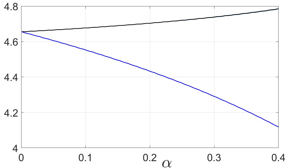
Figure 1: The integral $-\int_{0}^{\infty}\ln|T(\omega)|^{2}\omega^{-2}{\operatorname{d}\omega}$ for the attenuation model of Eq. (34). The upper (black) curve is actually two close to one another, one determined using numerical integration, the other from the expression in Eq. (33). The lower (blue) curves use the expression in Eq. (30) which does not account for damping.

IV.3 Reflection from a slab with rigid or free backing

A reflected delta pulse signal $s(t)=\delta(t)$ has zero delay because of the instantaneous wavefront interaction at the interface. The associated minimum phase function therefore has no phase delay but it does involve an all-pass filter associated with the zeros $\omega_{j}$ of $R(\omega)$ in the upper half plane,

$$R_{\text{mp}}(\omega)=R(\omega)/\prod_{j}Z(\omega,\omega_{j}).$$ (35)

Let $R(\omega)=R_{0}+\mathrm{i}\omega R_{1}+\ldots$, then

$$R_{\text{mp}}(\omega)=R_{\text{mp},0}+\mathrm{i}\omega R_{\text{mp},1}+\ldots,$$ (36)

where

$$R_{\text{mp},0} =Z_{0}R_{0},$$ (37)

$$R_{\text{mp},1} =Z_{0}\Big{(}R_{1}+2R_{0}\sum_{j}\operatorname{Im}\frac{1}{\omega_{j}}\Big{)}$$

and $Z_{0}=\prod_{n}(\omega_{n}^{*}/\omega_{n})$. The constraints on $\{\omega_{n}\}$ imply that $Z_{0}=1$ or $Z_{0}=-1$. In the next examples we consider the limiting cases for which $R_{0}=\pm 1$.

IV.3.1 Rigid backing

For the rigid backing, Lemma 1 and Eqs. (37), (57b) imply using $S(\omega)=\ln\big{(}Z_{0}R_{\text{mp}}(\omega)\big{)}$ that

$$-\int_{0}^{\infty}\ln|R(\omega)|^{2}\frac{\operatorname{d}\omega}{\omega^{2}}=\frac{2\pi a}{c}\frac{\langle C_{0}^{\prime}\rangle}{C}+2\pi\sum_{j}\operatorname{Im}\frac{1}{\omega_{j}}$$ (38)

in agreement with (Yang2017, , Eq. (A9)) and (Yang2017a, , Eq. (S9)).

Alternatively, taking $S(\omega)=R(\omega)-1$, Lemma 1 and Eq.  (57b) yield

$$\int_{0}^{\infty}\operatorname{Re}\big{(}1-R(\omega)\big{)}\frac{\operatorname{d}\omega}{\omega^{2}}=\frac{\pi a}{c}\frac{\langle C_{0}^{\prime}\rangle}{C}.$$ (39)

IV.3.2 Soft backing

For the soft backing, Lemma 1 and Eqs.  (37), (57c) imply using $S(\omega)=\ln[-Z_{0}R_{\text{mp}}(\omega)]$ that

$$-\int_{0}^{\infty}\ln|R(\omega)|^{2}\frac{\operatorname{d}\omega}{\omega^{2}}=\frac{2\pi a}{c}\frac{\langle\rho_{0}^{\prime}\rangle}{\rho}+2\pi\sum_{j}\operatorname{Im}\frac{1}{\omega_{j}}.$$ (40)

Alternatively, taking $S(\omega)=R(\omega)+1$, Lemma 1 and Eq.  (57c) yield

$$\int_{0}^{\infty}\operatorname{Re}\big{(}1+R(\omega)\big{)}\frac{\operatorname{d}\omega}{\omega^{2}}=\frac{\pi a}{c}\frac{\langle\rho_{0}^{\prime}\rangle}{\rho}.$$ (41)

V Discussion: Connection with the mass law

The main results are new integral identities (24) and (30) for the reflection and transmission coefficients of a slab in an infinite medium, and Eqs.  (39) - (41) for reflection from a slab with a rigid or soft backing. The general methodology has also been used to derive two previously known identities: (20) for the integrated extinction and (38) for the slab with rigid backing.

It is important to point out that all of these results include the possibility of energy loss through material damping. However, many of the integral identities depend only on the limiting static values of the density and bulk modulus, e.g. Eq.  (20) for the IE, and Eqs. (24), (39), (41) for reflection coefficients. These identities are therefore independent of the particular damping mechanisms present, an unexpected and surprising result. The identity (33) for the integrated transmission loss depends not only on the static values of the slab parameters but also on the infinite frequency value of the wave speed, which cannot be less than the zero frequency speed.

The identities (38) and (40) involve the complex-valued zeros $\{\omega_{j}\}$ which do depend on the material damping. In the absence of absorption, since the slab is backed by a perfect reflector it follows that $|R(\omega)|=1$ in both cases. The integrals (38) and (40) are therefore zero, with the right hand sides implying two identities for the quantities $\sum_{j}\operatorname{Im}\frac{1}{\omega_{j}}$. When damping is present the integrals represent the loss of acoustic energy into the slab over all frequencies. This was the motivation for the original derivation Yang2017 ; Yang2017a of (38).

Finally we note an interesting connection between the exact identity (30) for the integrated transmission loss of a uniform slab with no damping,

$$-\int_{0}^{\infty}\ln|T(\omega)|^{2}\frac{\operatorname{d}\omega}{\omega^{2}}=\frac{\pi a\rho^{\prime}}{2c\rho}\Big{(}1-\frac{z}{z^{\prime}}\Big{)}^{2}$$ (42)

and the same integral using a well known and useful approximation for $T(\omega)$. The transmission coefficient using the ”mass law” (KinslerFrey, , §6.7) is

$$T_{\text{mass}}(\omega)=\frac{1}{1-\mathrm{i}\frac{\omega a\rho^{\prime}}{2c\rho}}.$$ (43)

This yields an integrated transmission loss

$$-\int_{0}^{\infty}\ln|T_{\text{mass}}(\omega)|^{2}\frac{\operatorname{d}\omega}{\omega^{2}}=\frac{\pi a\rho^{\prime}}{2c\rho}$$ (44)

clearly a good approximation to the exact ITL (42) if $z^{\prime}\gg z$, which is implicitly assumed in the mass law approximation. It is interesting to note that the simple mass law approximation captures the full frequency content of the integrated transmission loss.

This all suggests a slight modification of the mass law,

$$T_{\text{approx}}(\omega)=\frac{1}{1-\mathrm{i}\frac{\omega a\rho^{\prime}}{2c\rho}\big{(}1-\frac{z}{z^{\prime}}\big{)}^{2}}.$$ (45)

The proposed transmission coefficient has several benefits including that it is unity if the impedances are equal, as it should. It also reproduces the integrated loss (42) exactly. However, the mass law in its simple or modified form cannot be expected to accurately reproduce the ITL for a slab with absorption, Eq. (33), since the approximations (43) and (45) for the transmission coefficient use static quantities only.

Acknowledgments

Thanks to Allan P. Rosenberg and to the reviewers for comments. This work was supported under the National Science Foundation Award No. EFRI 1641078 and the ONR MURI Grant No. N000141310631.

Appendix A Integral identities for real causal signals

The $\omega-$functions $S(\omega)$, $1/(\omega-\zeta)$ are both transforms of causal signals, and therefore so are $S(\omega)/(\omega-\zeta)$ and the subtraction function (Nuss72, , eq. (1.7.4))

$$S^{(1)}(\omega,\zeta)=\frac{S(\omega)-S(\zeta)}{\omega-\zeta}.$$ (46)

In this way we may form a chain of causal transforms: $S^{(n)}(\omega)$, $n=1,2,\ldots$

$$S^{(n+1)}(\omega,\zeta)=\frac{S^{(n)}(\omega,\zeta)-{\operatorname{d}^{n}}S(\omega)/{\operatorname{d}\omega^{n}}}{\omega-\zeta},\ \ n>1.$$ (47)

Being causal transforms, the Sokhotski-Plemelj relation (5) applies to each of the functions $S^{(n)}$,

$$S^{(n)}(\omega,\zeta)=\frac{1}{\mathrm{i}\pi}\mathchoice{{\vbox{\hbox{$\textstyle-$}}\kern-4.86108pt}}{{\vbox{\hbox{$\scriptstyle-$}}\kern-3.25pt}}{{\vbox{\hbox{$\scriptscriptstyle-$}}\kern-2.29166pt}}{{\vbox{\hbox{$\scriptscriptstyle-$}}\kern-1.875pt}}\!\int_{-\infty}^{\infty}S^{(n)}(\omega^{\prime},\zeta)\frac{\operatorname{d}\omega^{\prime}}{\omega^{\prime}-\omega}.$$ (48)

The limiting values of the $S^{(n)}$ functions as $\zeta\to\omega$ are

$$S^{(n)}(\omega,\omega)=\frac{1}{n!}\frac{\operatorname{d}^{n}S(\omega)}{\operatorname{d}\omega^{n}}$$ (49)

from which it follows that the $n-$th derivative of $S(\omega)$ can be expressed as an integral of lower order derivatives,

$$\frac{\operatorname{d}^{n}S(\omega)}{\operatorname{d}\omega^{n}}=\frac{n!}{\mathrm{i}\pi}\mathchoice{{\vbox{\hbox{$\textstyle-$}}\kern-4.86108pt}}{{\vbox{\hbox{$\scriptstyle-$}}\kern-3.25pt}}{{\vbox{\hbox{$\scriptscriptstyle-$}}\kern-2.29166pt}}{{\vbox{\hbox{$\scriptscriptstyle-$}}\kern-1.875pt}}\!\int_{-\infty}^{\infty}S^{(n)}(\omega^{\prime},\omega)\frac{\operatorname{d}\omega^{\prime}}{\omega^{\prime}-\omega}.$$ (50)

Specializing the Sokhotski-Plemelj relation (5) and the identities (50) to the case $\omega=0$ yields

$$S(0) =\frac{1}{\mathrm{i}\pi}\mathchoice{{\vbox{\hbox{$\textstyle-$}}\kern-4.86108pt}}{{\vbox{\hbox{$\scriptstyle-$}}\kern-3.25pt}}{{\vbox{\hbox{$\scriptscriptstyle-$}}\kern-2.29166pt}}{{\vbox{\hbox{$\scriptscriptstyle-$}}\kern-1.875pt}}\!\int_{-\infty}^{\infty}S(\omega)\frac{\operatorname{d}\omega}{\omega},$$ (51a)

$$S^{\prime}(0) =\frac{1}{\mathrm{i}\pi}\mathchoice{{\vbox{\hbox{$\textstyle-$}}\kern-4.86108pt}}{{\vbox{\hbox{$\scriptstyle-$}}\kern-3.25pt}}{{\vbox{\hbox{$\scriptscriptstyle-$}}\kern-2.29166pt}}{{\vbox{\hbox{$\scriptscriptstyle-$}}\kern-1.875pt}}\!\int_{-\infty}^{\infty}\big{(}S(\omega)-S(0)\big{)}\frac{\operatorname{d}\omega}{\omega^{2}},$$ (51b)

$$S^{\prime\prime}(0) ={\frac{2}{\mathrm{i}\pi}}\mathchoice{{\vbox{\hbox{$\textstyle-$}}\kern-4.86108pt}}{{\vbox{\hbox{$\scriptstyle-$}}\kern-3.25pt}}{{\vbox{\hbox{$\scriptscriptstyle-$}}\kern-2.29166pt}}{{\vbox{\hbox{$\scriptscriptstyle-$}}\kern-1.875pt}}\!\int_{-\infty}^{\infty}\big{(}S(\omega)-S(0)-\omega S^{\prime}(0)\big{)}\frac{\operatorname{d}\omega}{\omega^{3}}\ldots.$$ (51c)

Finally, we restrict (51) to real causal signals for which we have the additional property $S(-\omega)=S^{*}(\omega)$. Using this and (3) the integrals (51) reduce to (6) .

Appendix B Layered one dimensional medium

The slab occupies $\Omega:x\in[0,a]$ with non-uniform density and compressibility $\rho^{\prime}(x,\omega)$, $C^{\prime}(x,\omega)$. The 2-vector of particle velocity and acoustic pressure ${\bf U}=\big{(}v,p\big{)}^{T}$ is propagated from one end to the other by the 2$\times$2 matrix ${\bf M}(x,\omega)$, $\det{\bf M}=1$, such that ${\bf U}(a)={\bf M}(a,\omega){\bf U}(0)$. The propagator satisfies (Pease, , §7)

$$\frac{\operatorname{d}{\bf M}}{\operatorname{d}x}(x,\omega)=i\omega{\bf Q}{\bf M},\ \ {\bf M}(0,\omega)={\bf I},$$ (52)

with ${\bf I}$ the identity and

$${\bf Q}(x,\omega)=\begin{pmatrix}0&C^{\prime}(x,\omega)\\ \rho^{\prime}(x,\omega)&0\end{pmatrix}.$$ (53)

The solution follows using well known methods for uni-dimensional systems, e.g. Ch. 7 of Pease Pease . The medium in $x<0$ ($x>a$) is assumed to have properties $z,c$ ($z_{1},c$), where the impedance $z_{1}$ is introduced to allow for different boundary conditions at $x=a$, specifically the cases of interest $z_{1}=z,\infty,0$.

The reflected and transmitted fields are

$$p(x)=\begin{cases}e^{\mathrm{i}kx}+Re^{-\mathrm{i}kx},&x<0,\\ Te^{\mathrm{i}kx},&x>a,\end{cases}$$ (54)

where $k=\omega/c$. Hence,

$$T =\frac{2\mathrm{e}^{-\mathrm{i}ka}}{M_{11}+zz_{1}^{-1}M_{22}-zM_{12}-z_{1}^{-1}M_{21}},$$ (55a)

$$R =\frac{M_{11}-zz_{1}^{-1}M_{22}+zM_{12}-z_{1}^{-1}M_{21}}{M_{11}+zz_{1}^{-1}M_{22}-zM_{12}-z_{1}^{-1}M_{21}},$$ (55b)

where $M_{ij}$ are the elements of ${\bf M}(a,\omega)$.

For our purposes, we note that at low frequency ${\bf M}(a,\omega)={\bf I}+i\omega a\langle{\bf Q}_{0}\rangle+...$ where $\langle\cdot\rangle$ denotes the average value in $\Omega$. Hence,

$$T =\frac{2z_{1}}{z_{1}+z}+\frac{\mathrm{i}ka2z_{1}^{2}}{(z_{1}+z)^{2}}\big{(}\frac{\big{\langle}C_{0}^{\prime}\rangle}{C}+\frac{z\langle\rho_{0}^{\prime}\rangle}{z_{1}\rho}-\frac{z}{z_{1}}-1\big{)}$$ (56)

$$+{\cal O}(\omega^{2}),$$

$$R =\frac{z_{1}-z}{z_{1}+z}+\frac{\mathrm{i}ka2z_{1}^{2}}{(z_{1}+z)^{2}}\big{(}\frac{\big{\langle}C_{0}^{\prime}\rangle}{C}-\frac{z^{2}\langle\rho_{0}^{\prime}\rangle}{z_{1}^{2}\rho}\big{)}+{\cal O}(\omega^{2}).$$

The three cases of interest are (i) the slab sandwiched by the same material on either side, (ii) the slab with a rigid backing, and (iii) the slab with a soft boundary on one side, or respectively

$$\left.\begin{aligned} T&=1+\frac{\mathrm{i}ka}{2}\Big{(}\frac{\big{\langle}C_{0}^{\prime}\rangle}{C}+\frac{\langle\rho_{0}^{\prime}\rangle}{\rho}-2\Big{)}+{\cal O}(\omega^{2}),\\ R&=\frac{\mathrm{i}ka}{2}\Big{(}\frac{\big{\langle}C_{0}^{\prime}\rangle}{C}-\frac{\langle\rho_{0}^{\prime}\rangle}{\rho}\Big{)}+{\cal O}(\omega^{2}),\end{aligned}\right\}\ \ z_{1}=z,$$ (57a)

$$R=1+\mathrm{i}ka2\frac{\langle C_{0}^{\prime}\rangle}{C}+{\cal O}(\omega^{2}),\ \ z_{1}=\infty,$$ (57b)

$$R=-1-\mathrm{i}ka2\frac{\langle\rho_{0}^{\prime}\rangle}{\rho}+{\cal O}(\omega^{2}),\ \ z_{1}=0.$$ (57c)

Finally, note that damping may be included by considering the material properties as frequency dependent complex parameters. In that case $\langle\cdot\rangle$ is the spatial average of the real valued static quantity $(\omega=0)$.

References

• (1) E. M. Purcell. On the absorption and emission of light by interstellar grains. Astrophys. J., 158:433–440, 1969.
• (2) Christian Sohl, Mats Gustafsson, and Gerhard Kristensson. Physical limitations on broadband scattering by heterogeneous obstacles. J. Phys. A: Math. Theor., 40(36):11165–11182, Aug 2007.
• (3) Francesco Monticone and Andrea Alù. Do cloaked objects really scatter less? Phys. Rev. X, 3:041005+, July 2013.
• (4) C. Sohl, M. Gustafsson, and G. Kristensson. The integrated extinction for broadband scattering of acoustic waves. Journal of the Acoustical Society of America, 122(6):3206–3210, 2007.
• (5) A. N. Norris. Acoustic integrated extinction. Proc. R. Soc. A, 471(2177):20150008+, Apr 2015.
• (6) Min Yang and Ping Sheng. Sound absorption structures: From porous media to acoustic metamaterials. Annual Review of Materials Research, 47(1):83–114, jul 2017.
• (7) Min Yang, Shuyu Chen, Caixing Fu, and Ping Sheng. Optimal sound-absorbing structures. Materials Horizons, 4(4):673–680, 2017.
• (8) K.N. Rozanov. Ultimate thickness to bandwidth ratio of radar absorbers. IEEE Transactions on Antennas and Propagation, 48(8):1230–1234, 2000.
• (9) R. M. Fano. Theoretical limitations on the broadband matching of arbitrary impedances. J. Franklin Inst., 249:57–83, 1950.
• (10) H. M. Nussenzveig. Causality and dispersion relations. Academic, London, 1972.
• (11) Jonathan D. Victor. Temporal impulse responses from flicker sensitivities: causality, linearity, and amplitude data do not determine phase. Journal of the Optical Society of America A, 6(9):1302, sep 1989.
• (12) J. Gregory McDaniel. Applications of the causality condition to one-dimensional acoustic reflection problems. Journal of the Acoustical Society of America, 105(5):2710–2716, May 1999.
• (13) J. Gregory McDaniel and Cory L. Clarke. Interpretation and identification of minimum phase reflection coefficients. The Journal of the Acoustical Society of America, 110(6):3003–3010, dec 2001.
• (14) G. Dassios and R. Kleinman. Low frequency scattering. Oxford: Oxford University Press, 2000.
• (15) Lord Rayleigh. Theory of Sound, Vol. II. MacMillan and Company, Ltd, 1878.
• (16) C. Zener. Elasticity and Anelasticity of Metals. University of Chicago Press, Chicago, 1948.
• (17) Lawrence E. Kinsler, Austin R. Frey, Alan B. Coppens, and James V. Sanders. Fundamentals of Acoustics. Wiley, fourth edition, December 2000.
• (18) M. C. Pease. Methods of Matrix Algebra. Academic Press, New York, 1965.