Mapping the Interstellar Magnetic Field Around the Heliosphere with Polarized Starlight

Abstract

Starlight that becomes linearly polarized by magnetically aligned dust grains provides a viable diagnostic of the interstellar magnetic field (ISMF). A survey is underway to map the local ISMF using data collected at eight observatories in both hemispheres. Two approaches are used to obtain the magnetic structure: statistically evaluating magnetic field directions traced by multiple polarization position angles, and least-squares fits that provide the dipole component of the magnetic field. We find that the magnetic field in the circumheliospheric interstellar medium (CHM), which drives winds of interstellar gas and dust through the heliosphere, drapes over the heliopause, and influences polarization measurements. We discover a polarization band that can be described with a great circle that traverses the heliosphere nose and ecliptic poles. A gap in the band appears in a region coinciding both with the highest heliosheath pressure, found by IBEX, and the center of the Loop I superbubble. The least-squares analysis finds a magnetic dipole component of the polarization band with the axis oriented toward the ecliptic poles. The filament of dust around the heliosphere and the warm helium breeze flowing through the heliosphere trace the same magnetic field directions. Regions along the polarization band near the heliosphere nose have magnetic field orientations within 15^∘ of sightlines. Regions in the IBEX ribbon have field directions within 40^∘ of the plane of the sky. Several spatially coherent magnetic filaments are within 15 pc. Most of the low frequency radio emissions detected by the two Voyager spacecraft follow the polarization band. The geometry of the polarization band is compared to the Local Interstellar Cloud, the Cetus Ripple, the BICEP2 low opacity region, Ice Cube IC59 galactic cosmic ray data, and Cassini results.

1 Introduction

Spatial inhomogeneities in the nearby interstellar magnetic field and gas modulate the heliosphere during the solar motion through space. The distribution, kinematics and pressure of gas in the cluster of local interstellar clouds (CLIC) through which the Sun is traveling is moderately well known, having been studied with interstellar absorption lines for the past century (Heger, 1919). Mapping the magnetic field in the low density very local interstellar medium has only recently become possible with the development of high-precision polarimeters. With the goal of relating the local interstellar magnetic field to the magnetic field shaping the heliosphere, we are mapping the configuration of the local interstellar magnetic field utilizing starlight that is polarized by magnetically-aligned interstellar dust grains. The interstellar polarizations discussed in this paper arise from dust grains located in the CLIC, some of which are swept up into and around the heliosphere. This study focuses on the magnetic field configuration within 15 pc. Interstellar gas in this region is warm, low density, and kinematically structured with a tendency to flow away from the direction of the center of the Loop I superbubble (Frisch et al., 2011, FRS11). The polarized starlight data utilized here include newly-collected measurements that have been acquired at eight observatories in both hemispheres.

The relation between the interstellar magnetic field that shapes the heliosphere and the ambient interstellar magnetic field is key to understanding the physical properties of the immediate galactic environment of the Sun. Polarized starlight has been shown to provide a viable diagnostic of the orientation and structure of the local interstellar magnetic field over both large and small spatial scales (e.g. Mathewson & Ford, 1970; Piirola, 1977; Tinbergen, 1982; Pereyra & Magalhães, 2007; Bailey et al., 2010; Frisch et al., 2012; Berdyugin et al., 2014; Wiktorowicz & Nofi, 2015; Frisch et al., 2015b, a; Cotton et al., 2016; Marshall et al., 2016; Cotton et al., 2017b). Stars within 40 pc show interstellar linear polarizations of $\sim 0.0004\%$/pc or less, corresponding to mean densities of n(H^o)$\sim 0.08$ cm^-3, with a tendency for larger polarizations in southern compared to northern galactic regions (Piirola, 1977; Tinbergen, 1982; Marshall et al., 2016; Cotton et al., 2017b). In this study the magnetic field orientations are explicitly assumed to be parallel to the position angles of the linearly polarized starlight, so that possible radiative torques would affect the efficiency of grain alignment but not the alignment orientation (Hoang & Lazarian, 2016).

Local space is sparsely filled with interstellar material so that polarizing dust grains may be entrained in multiple magnetic fields that are foreground to nearby stars. For volume densities similar to the densities of the interstellar material entering the heliosphere, n(H^o)$\sim 0.2$ cm^-3 and n_e$\sim 0.07$ cm^-3, and typical column densities N(H^o)$\sim 10^{17.6}$ cm^-2, and cloud lengths are less than 1 pc (FRS11). A kinematical model of the CLIC as consisting of fifteen clouds predicts that less than 19% of nearby space is filled with gas (Redfield & Linsky, 2008a). Interstellar gas absorption components detected toward individual nearby stars indicate filling factors of 5%–40% (Frisch & Slavin, 2006). These low cloud filling factors suggest that the polarizing interstellar dust grains are distributed over less than 20% of local interstellar space.

Heliospheric data have recently provided an entirely new perspective of the CircumHeliospheric interstellar Medium (CHM) forming the interstellar boundary conditions of the heliosphere. The CHM establishes the interstellar boundary conditions of the heliosphere, feeds interstellar gas and dust into the heliosphere, and absorbs the escaping energetic neutral atoms (ENAs) that were created by charge-exchange between the solar wind and CHM neutral gas inside of the heliosphere. In situ measurements of interstellar He^∘ in the inner heliosphere by Ulysses and the Interstellar Boundary Explorer (IBEX) give an upwind direction for the CHM velocity of $\ell$=3.7^∘, $b$=15.1^∘, and low volume densities of n(He^o)=0.0196$\pm 0.0033$ cm^-3 (Schwadron et al., 2015a; Wood et al., 2017). The angle between the CHM and LIC velocity vectors is $4.3^{\circ}\pm 2.6^{\circ}$.

An unexpected tracer of the interstellar magnetic field embedded in the CHM was provided by the discovery of a “ribbon” of ENAs forming where the local interstellar magnetic field (ISMF) draping over the heliosphere is perpendicular to sightlines (McComas et al., 2009; Schwadron et al., 2009; Funsten et al., 2009; Fuselier et al., 2009). MHD simulations of the ribbon origin predict that ribbon ENAs are born 10 AU or more upstream of the heliopause, depending on the ENA energies (Zirnstein et al., 2016). The center of the $\sim 73$^∘-radius circular ENA ribbon provides the energy-dependent orientation of the magnetic field in the CHM. An angle of $88^{\circ}\pm 3^{\circ}$ is found between the CHM velocity in the Local Standard of Rest (LSR), and the interstellar magnetic field direction traced by the IBEX ribbon, based on in situ He^∘ data and the magnetic field orientation of the CHM from the 1 keV ribbon, indicating the CHM velocity and magnetic field are perpendicular (Schwadron et al., 2014a). The secondary population of heated interstellar He^∘ atoms, consisting partly of interstellar ions that are deflected in the outer heliosheath, become re-neutralized and are measured in the inner heliosphere (Kubiak et al., 2014, 2016; Bzowski et al., 2017). The direction of this secondary neutral “breeze” traces the magnetic distortion of the heliosphere.

The Sun is at the edge of the CHM in the upwind direction of the interstellar neutral wind. Absorption components at the CHM or LIC velocities are not detected toward 36 Oph in the upwind direction (Wood et al., 2000), or toward the nearest star $\alpha$ Cen, 49^∘ from the heliosphere nose (Lallement et al., 1995; Gayley et al., 1997). Voyager 1 crossed the heliopause at 122 AU in August of 2012 and is acquiring in situ data on the interstellar magnetic field (Burlaga & Ness, 2014, 2016). A laminar magnetic field with Gaussian turbulence was detected in the outer heliosheath during periods outside of solar magnetic storms, and was identified as the interstellar magnetic field (Burlaga & Ness, 2014). The gradient of the interstellar magnetic field detected by Voyager 1 during the first quiet time beyond the heliopause, uninterrupted by solar storms, was found to converge on the interstellar magnetic field orientation given by the center of the IBEX ribbon (Schwadron et al., 2015b). The low levels of magnetic turbulence detected in the heliosheath by Voyager 1 beyond the heliopause at 135 AU is consistent with Kolmogorov turbulence with an outer scale of 0.01 pc, indicating the spacecraft and heliosphere are near the cloud edge (Burlaga et al., 2018).

We find here that interstellar dust grains interacting with the heliosphere affect linearly polarized starlight data. In situ dust measurements indicate that interstellar dust interacts with and is deflected around the heliosphere (e.g. Frisch et al., 2005; Mann, 2010). The interstellar gas and dust inside of the heliosphere have the same velocity vectors (Frisch et al., 1999; Kimura et al., 2003). Ulysses and Galileo data show that grains with the largest charge-to-dust mass ratios are excluded from the inner heliosphere and indicate gas-to-dust mass ratios of 192 (+85,-57), vs. typical interstellar values of 100 (Frisch et al., 1999; Krüger et al., 2015; Sterken et al., 2015). The grains have silicate compositions, based on the composition of the gaseous CHM and in situ dust measurements (Slavin & Frisch, 2008; Altobelli et al., 2016). Detailed interactions between interstellar dust grains and the heliosphere depend on the magnetic phase of the Hale solar cycle due to Lorentz forces on charged grains in the heliosheath (Frisch et al., 1999; Landgraf et al., 1999; Mann & Czechowski, 2004; Slavin et al., 2012; Sterken et al., 2015; Alexashov et al., 2016). The spectrum of locally polarized starlight is bluer than that of more obscured distant stars, suggesting the presence of smaller grains (Marshall et al., 2016).

Measurements by Voyagers 1 and 2 inside of the heliosphere identified low frequency radio emissions upstream of the heliopause that are associated with disturbances of the interstellar plasma and magnetic field (Gurnett et al., 1993; Kurth & Gurnett, 2003). The heliopause crossing was also marked by the reappearance of low frequency radio plasma emissions at the plasma frequency of an interstellar electron population with density 0.08 cm^-3 (Gurnett et al., 2013).

Here we use a statistical approach for defining structure in the ISMF traced by the polarization data. Earlier efforts to obtain the orientation of the very local interstellar magnetic field from linear polarization data found an ISMF direction consistent with the IBEX ribbon magnetic field direction, after omitting a data subset that appears to define a filament of polarizing dust grains around the heliosphere (Frisch et al., 2015a, b). The coincidence of the magnetic field traced by the dust filament and the direction of the “warm breeze” of secondary interstellar helium discovered by IBEX is confirmed in this paper.

Achieving our goal of mapping the interstellar magnetic field in the very low column density of the local interstellar medium is possible only because of recent advances in precision polarimetry that give accuracies of parts-per-million (Magalhaes et al., 1996; Wiktorowicz & Matthews, 2008; Bailey et al., 2010; Piirola et al., 2014; Bailey et al., 2015, 2017). In this paper we combine older less precise 20th century data (Heiles, 2000) with high precision polarization measurements made in the 21st century in order to probe the geometrical properties of the interstellar magnetic field within 15 pc. These results are built on combining polarization position angles based on methods introduced in Frisch et al. (2016), and on a classic least-squares-fit analysis. The analysis in this paper is restricted to stars within $\sim 15$ pc, where interstellar column densities are low.

Data used here are summarized in Section (§) 2. Polarization measurements of over 270 nearby stars made with the DIPOL-2 instrument (Piirola et al., 2014) have enabled this survey and are being published separately.The methodology for obtaining magnetic structure by counting the number of stars that predict magnetic fields at each location according to statistical criteria is explained in §3. Probability constraints permit sorting the magnetic structure maps according to whether polarization position angles trace magnetic field lines that are either quasi-parallel or quasi-perpendicular to the plane of the sky. A band of favored magnetic field directions is found (§3.1). Magnetic structure is sampled for intervals of $\pm 90^{\circ}$ (§3.2), and $\pm 60^{\circ}$ and $\pm 45^{\circ}$ (§3.3). A least-squares analysis was performed on the best data describing the polarization band, yielding a dipole component at the ecliptic poles (§4.1). A previously discovered filament of polarized interstellar dust grains (Frisch et al., 2015a) is re-examined with a least-squares analysis (§4.2), confirming a magnetic pole aligned with the direction of the warm breeze of secondary interstellar He^∘ (§4.2). Maps of mean polarization angles yields angles of the magnetic field throughout the sky (§5). The discussion (§6) relates magnetic structure to supplementary data on the outer heliosheath, including Voyager interstellar plasma emissions, the coincidence of the magnetic fields traced by the dust filament and warm breeze of secondary interstellar helium, as well as Loop I and southern TeV cosmic ray data. Concluding remarks are presented in §7. Table 1 summarizes locations quoted in this paper. Additional information on the statistical distributions, the polarization band and supplementary data, the relation between the polarization band and Cassini belt, and the spatial counting of target stars with the most detectable polarizations is given in Appendices A–D, respectively.

2 Polarization Data Used in Analysis

This study utilizes linearly polarized starlight as the basis of determining the structure of the nearest interstellar magnetic field. Starlight that is linearly polarized while traversing a dichroic interstellar medium created by magnetically aligned interstellar dust grains provides a longstanding diagnostic of the interstellar magnetic field orientation (e.g. Mathewson & Ford, 1970; Piirola, 1973; Serkowski et al., 1975). Linearly polarized starlight is parallel to the interstellar magnetic field direction in the absence of a strong local radiation source that can perturb (or enhance) alignment (see the review of Andersson et al., 2015). Linear polarizations are derived from measurements of the Q and U Stokes parameters, which yield polarization position angles $\theta_{\mathrm{PA}}$ (the angle between the meridian of the coordinate system and the polarization pseudo-vector) and their uncertainties ($\delta\theta_{\mathrm{PA}}$, e.g. Tinbergen, 1982; Naghizadeh-Khouei & Clarke, 1993; Plaszczynski et al., 2014).

Observed orientations of the polarization position angles, $\theta_{\mathrm{PA}}$, represent the projection onto the plane of the sky of the three-dimensional linearly polarized pseudo-vector, and is regarded as insensitive to the polarity of the interstellar magnetic field. In principle the observed polarization strength will decrease with the angle between the star and the location where the magnetic field is perpendicular to the plane of the sky. In this study we utilize polarization position angles to map the structure of the nearby interstellar magnetic field. Polarization strengths are not directly utilized in this study because of the heterogeneous underlying data that are drawn from diverse sources with variable sensitivity levels, some collected during the 20th century (Piirola, 1977; Tinbergen, 1982; Leroy, 1993; Heiles, 2000).

The development of high sensitivity polarimeters has allowed the precise measurements of starlight polarizations arising in the low column density nearby interstellar material where typically N(H^o+H⁺) $\sim 10^{17}-10^{18.5}$ cm^-2 (Wood et al., 2005), corresponding to expected polarization strengths of 0.0002%–0.005% compared to mean measurement errors of parts-per-million or better.

This study includes essential new data that have been acquired for this survey of interstellar polarizations in the local interstellar medium using the DiPol-2 polarimeter (Piirola et al., 2014). This instrument yields high precision polarization measurements at better than $10^{-5}$ levels. Three copies of DIPOL-2 have been built and are being used at the UH88 telescope at Mauna Kea Observatory, the T60 telescope at Haleakala Observatory, and the 1.3 m telescope of the Greenhill Observatory (H127), University of Tasmania, Australia. Additional new data have been obtained with IAGPOL (Magalhaes et al., 1996) at the Pico dos Dias Observatory in Brazil. These new data from the DIPOL-2 instrument are being published separately (Berdyugin et al., in preparation; Frisch et al., in preparation).

Data from the literature on the polarizations of nearby stars are also used in this study (Bailey et al., 2010; Santos et al., 2011; Frisch et al., 2012, 2015b, 2015a; Bailey et al., 2015; Wiktorowicz & Nofi, 2015; Marshall et al., 2016; Cotton et al., 2016, 2017b; Bailey et al., 2017). Data from the literature include high precision data collected at Lick Observatory in California, at the Anglo-Australian Telescope at Siding Spring Observatory in Australia, and at the 14” telescope at the UNSW observatory at the Kensington campus in Australia.

The analysis in this paper is based on stars with distances within 15 pc, where a star is considered to be within 15 pc if any part of the parallax error conical section is less than 16.0 pc. This requirement is the only distance information utilized in this paper. Stellar distances are available for all of the stars included in this analysis, and are determined from Hipparcos parallax data (Perryman, 1997) by utilizing the parallax uncertainties to identify the distance that divides the volume of the parallax uncertainty conical section into two equal volumes. The current polarization data base consists of measurements of the polarizations of over 760 stars within 40 pc, of which 134 stars are utilized in this study.

Newly acquired data for this survey avoid known intrinsically polarized stars, and binary systems where intrinsic polarization may be present (see Cotton et al., 2017b, for a discussion of intrinsic stellar polarizations), however it is likely that intrinsically polarized stars remain in the data set utilized in this paper. In the present analysis it is assumed that intrinsically polarized stars, if present, would contribute randomly oriented polarization position angles that would not bias the results. Polarization strengths are not used directly in this study but will affect uncertainties on the polarization position angles (Appendix A). The merit function used to determine the probabilities, $\Gamma$(L_rot,B_rot), is based on the probability distribution for polarization position angles given by Naghizadeh-Khouei & Clarke (1993, Appendix A). An upper limit of 3.5 is therefore placed on the probabilities $\Gamma$(L_rot,B_rot) that are incorporated into the calculation of the statistical significance of individual data points. This limit, which affects 16% of the stars utilized in this study, is required to minimize the influence of possible intrinsic stellar polarizations that could mimic interstellar polarizations and bias outcomes.

The physical distribution of the stars in the sky is unrelated to the magnetic structure derived in this paper. For instance, compare the distributions of stars in Appendix B with the magnetic structure maps presented here.

3 Mapping Magnetic Structure with Polarization Position Angles

Starlight that becomes linearly polarized while traversing a dichroic medium formed by magnetically aligned dust grains provides the basis for determining the structure of the local interstellar magnetic field. Magnetic fields in regions devoid of interstellar dust will not be sampled in this analysis. Three approaches are used here to map the structure of the local interstellar magnetic field using polarization position angle data. The first approach (this section) is based on counting the number of overlapping polarization position angle (PPA) swaths that trace a “true” magnetic field towards each location on the sky according to statistical criteria, and normalizing that count by the number of stars within $\alpha_{\mathrm{max}}$ degrees of that location, and then characterizing the magnetic field orientation using patterns of those counts on the sky (Frisch et al., 2016). The approach imposes either minimum or maximum limits on the values of $\Gamma$(L_rot,B_rot) that will be mapped at each location, in an approach that is conceptually analogous to binning the data according to the statistical probabilities. The second approach (§4) is a least-squares analysis that finds the most probable location for the dipole component of the magnetic poles traced by the polarization position angles of the stars tracing the polarization band feature (§4.1), and the polarization filament (§4.2). In the third approach we map the mean values of $\theta_{\mathrm{rot}}$ at each position on the sky.

The method presented here for identifying structure in the interstellar magnetic field is based on the statistical probability that a polarization position angle will trace a magnetic field directed toward any location on the sky for a grid of longitudes $L_{\mathrm{rot}}$ and latitudes $B_{\mathrm{rot}}$, and then mapping the number of data points at each grid point that meet the statistical criterion for that map, after normalization by the total number of data points available for mapping at that location according to the geometrical constraints.

The statistical probability that a polarization position angle traces a magnetic field oriented toward $L_{\mathrm{rot}}$, $B_{\mathrm{rot}}$ is denoted $\Gamma$(L_rot,B_rot). The value for $\Gamma$(L_rot,B_rot) is derived by first calculating the angle between the polarization orientation and a meridian that passes through the location $L_{\mathrm{rot}}$, $B_{\mathrm{rot}}$. The statistical probability that $\theta_{\mathrm{rot}}$ traces a “true” magnetic field direction is then given by the probability distribution for position angles and measurement uncertainties. Appendix A shows this probability distribution for several levels of measurement uncertainties.

Two types of statistical limits are placed on $\Gamma$(L_rot,B_rot) values that constrain the plotted PPA values. The selection of data that will trace magnetic field directions that are quasi-parallel to the sightline requires that $\Gamma$(L_rot,B_rot), is large so that $\theta_{\mathrm{rot}}$ has a high probability of tracing a magnetic field with that orientation. The limits on the values of $\Gamma$(L_rot,B_rot) that are counted and plotted therefore restrict the orientations of the magnetic field lines that will be plotted. Magnetic field orientations that are quasi-parallel to the sightline are analogous to a dipole field with an orientation approximately aligned with the sightline with respect to the location $L_{\mathrm{rot}}$, $B_{\mathrm{rot}}$. Orientations quasi-perpendicular to the sightlines are closer to the plane of the sky. These different magnetic field orientations are implemented with the criteria $\Gamma$(L_rot,B_rot)$>$$\Gamma_{\mathrm{min}}$ for field directions quasi-parallel to the sightline, and $\Gamma$(L_rot,B_rot)$<$$\Gamma_{\mathrm{max}}$ for field directions quasi-perpendicular to the sightline. The values of $\Gamma_{\mathrm{min}}$ and $\Gamma_{\mathrm{max}}$ are selected to yield samples of the data large enough to cover all of the sky for the spatial constraints imposed on the map construction. These maps of the number of stars meeting the assumed statistical criteria then becomes the diagnostic of structure in the interstellar magnetic field. The parameters $L_{\mathrm{rot}}$, $B_{\mathrm{rot}}$ serve both to define the grid over which the magnetic field structure is plotted and the pole of the meridian that must be used for calculating the rotated polarization position angles, $\theta_{\mathrm{rot}}$. Note that polarization position angles are generally calculated with respect to meridians of either the equatorial ($\theta_{\mathrm{ra}}$) or galactic ($\theta_{\mathrm{gal}}$) coordinate systems, however they can be rotated into any spherical coordinate system defined by an arbitrary pole location $L_{\mathrm{rot}}$, $B_{\mathrm{rot}}$, to yield the value $\theta_{\mathrm{rot}}$ evaluated with respect to that rotated coordinate system.

A second geometric requirement is imposed that requires stars to be located within $\alpha_{\mathrm{max}}$ degrees of $L_{\mathrm{rot}}$, $B_{\mathrm{rot}}$ to be included in the plots. The number of data points that statistically qualify to be plotted is normalized by the total number of data points that satisfy the geometric criteria, e.g. the number of stars meeting the statistical criterion at $L_{\mathrm{rot}}$,$B_{\mathrm{rot}}$ is divided by the total number stars within 60^∘ of that location for the geometric criterion $\alpha_{\mathrm{max}}$$<$60^∘. Normalization compensates for the uneven spatial distribution of stars in the polarization data set, and has little effect on the $\alpha_{\mathrm{max}}$=90^∘ maps but is significant for the higher resolution maps at $\alpha_{\mathrm{max}}$=60^∘ and 45^∘ (§3.3).

Mapping magnetic structure is implemented by rotating the coordinate system through all possible poles for $L_{\mathrm{rot}}$, $B_{\mathrm{rot}}$, evaluating $\theta_{\mathrm{rot}}$ at each location for stars satisfying the geometric constraint. In §§3.1, 3.2, and 3.3 data are counted and plotted that meet the statistical requirement on $\theta_{\mathrm{rot}}$ after normalizing by the number of stars that meet the geometric constraint. Values of $\theta_{\mathrm{rot}}$ are small when they trace true interstellar magnetic field orientations that are nearly parallel to a meridian of the spherical coordinate system defined by a pole at $L_{\mathrm{rot}}$,$B_{\mathrm{rot}}$.

Maps built on the statistical requirement $\Gamma$(L_rot,B_rot)$>$$\Gamma_{\mathrm{min}}$ are unaffected by data points with low $P$/$dP$ for reasonable values of $\Gamma_{\mathrm{min}}$. Maps built on $\Gamma$(L_rot,B_rot)$<$$\Gamma_{\mathrm{max}}$ would not display correct magnetic structure for stars that lack foreground interstellar dust grains. Therefore, maps built using the condition $\Gamma$(L_rot,B_rot)$<$$\Gamma_{\mathrm{min}}$ also require that $P$/$dP$$>1.9$ in order to avoid confusing magnetic structure with stars devoid of foreground dust grains.

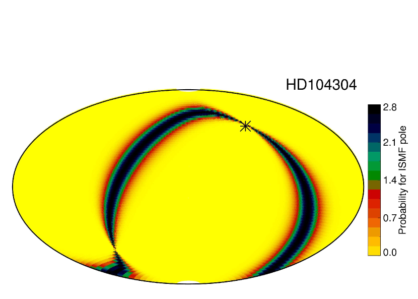
Figure 1: The color scale displays values of the probabilities, $\Gamma$(L_rot,B_rot), for measured polarization position angle, $\theta_{\mathrm{PA}}$, of the star HD 104304 to trace a magnetic field located at each position on the sky, $L_{\mathrm{rot}}$,$B_{\mathrm{rot}}$. The non-zero values of $\Gamma$(L_rot,B_rot) create the probability swath that will be sampled according to the probability constraints imposed on each calculation. HD 104304 is 13 pc away and located at $\ell$,$b$=283^∘,50^∘. DIPOL-2 measurements determine a polarization strengths of $P$=$0.0033\pm 0.0006$ percent. $\Gamma$(L_rot,B_rot) is zero at the position of the star because linear polarizations are parallel to the ISMF direction and can not be measured where the ISMF is inclined by 90^∘ with respect to the plane of the sky, so that the interstellar linear polarization vanishes for a star located at the magnetic pole. These data were acquired with DIPOL-2 mounted at T60 at the Haleakala Observatory. This figure and other maps in this paper are displayed using an Aitoff projection.

An example of a probability swath of possible magnetic pole locations is shown in Figure 1 for the star HD 104304, located $12.9\pm 1.0$ pc away at $\ell$,$b$=283^∘,50^∘. The HD 104304 data were obtained with the DIPOL-2 polarimeter at the T60 telescope at Haleakala. HD 104304 has a polarization position angle of $\theta_{\mathrm{ra}}$=$59.4^{\circ}\pm 4.9^{\circ}$, which corresponds to a position angle in galactic coordinates of $\theta_{\mathrm{gal}}$=$41.5^{\circ}\pm 4.9^{\circ}$. Figure 1 and other maps in this paper utilize an Aitoff projection.

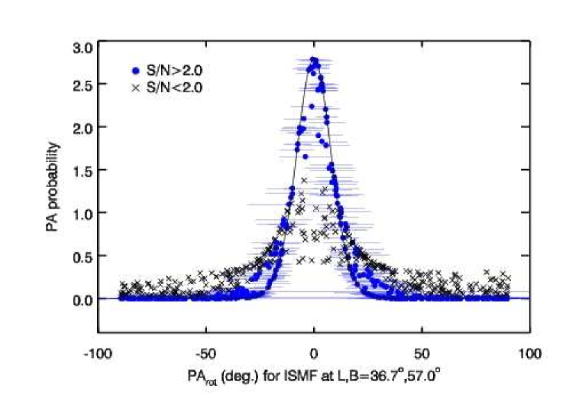
Figure 2: The probabity distribution $G_{\mathrm{n}}(\theta_{\rm{obs}};~{}\theta_{\rm{o}},P_{\rm{o}})$ (eqn. A1) is shown for an ISMF located at the direction $\ell$=36.7^∘,$b$=56.0^∘, for polarization data of stars within 40 pc. This direction corresponds to the weighted mean value of the IBEX ribbon center (Table 1). Data with $P$/$dP$$>2.0$ ($<2.0$) are plotted with dots (X’s), respectively. The solid line indicates the underlying statistical probability distribution given by Naghizadeh-Khouei & Clarke (1993, and A1).

Figure 2 shows an example of maps of the probability distribution $\Gamma$(L_rot,B_rot), based on the polarization position angles of stars within 40 pc that trace a magnetic field orientation toward $\ell=36.7^{\circ},~{}b=57.0^{\circ}$, corresponding to the the weighted mean center of the IBEX ribbon energy bands (Funsten et al., 2013, Table1 ). This distribution shows polarization data for stars within 40 pc that have high, as well as low, probabilities for tracing the IBEX ISMF direction, indicating that multiple magnetic field orientations are found. Appendix A also shows an additional example of the statistical distributions for the polarization position angles of stars tracing a field direction at the location $\ell$=135^∘ and $b$=5^∘.

The use of polarization position angle uncertainty swaths introduces several intrinsic biases to the output maps. Measurements with larger values of $P$/$dP$ will have larger values of $\Gamma$(L_rot,B_rot) for some locations but will also tend to be counted at fewer grid locations because the angular extent of the uncertainty swath is smaller. In contrast, large numbers of data points with low $P$/$dP$, and therefore large angular uncertainty swaths, will enlarge the number of grid points where the individual data points are counted (according to requirement $\Gamma$(L_rot,B_rot)$>$$\Gamma_{\mathrm{min}}$) and therefore spatially blur the magnetic structure.

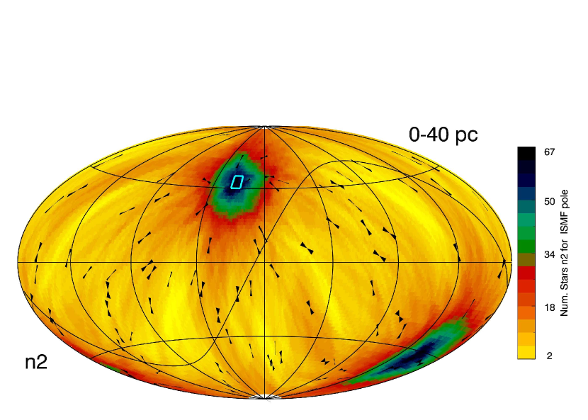
Figure 3: Examples of the construction of magnetic structure maps. Polarization data with values of $\theta_{\mathrm{rot}}$ satisfying the probability criteria $\Gamma$(L_rot,B_rot)$>$0.6 (left) or $\Gamma$(L_rot,B_rot)$>$0.9 (right) for tracing an ISMF direction located within the cyan-colored boxes are counted and mapped using the color-coding shown in the color-bar. Maps are centered on the galactic center with longitude increasing toward the left. The cyan-colored box is centered on the interstellar magnetic field direction affecting the IBEX ribbon configuration, $\ell$=$26.0^{\circ}\pm 0.7^{\circ}$, $b$=$50.1\pm 0.6^{\circ}$, as found by the Zirnstein et al. (2016) ribbon-formation simulations. Each measured polarization position angle creates a swath on the sky of magnetic field directions consistent with observed position angles $\theta_{\mathrm{PA}}$$\pm$$\delta\theta_{\mathrm{PA}}$ (see Figure 1). The black symbols indicate the directions of the polarization position angles and their uncertainties. The triangular uncertainties of the symbols illustrate the widths $\pm$$\delta\theta_{\mathrm{PA}}$ as plotted onto the Aitoff projection.

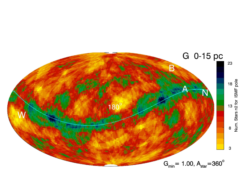
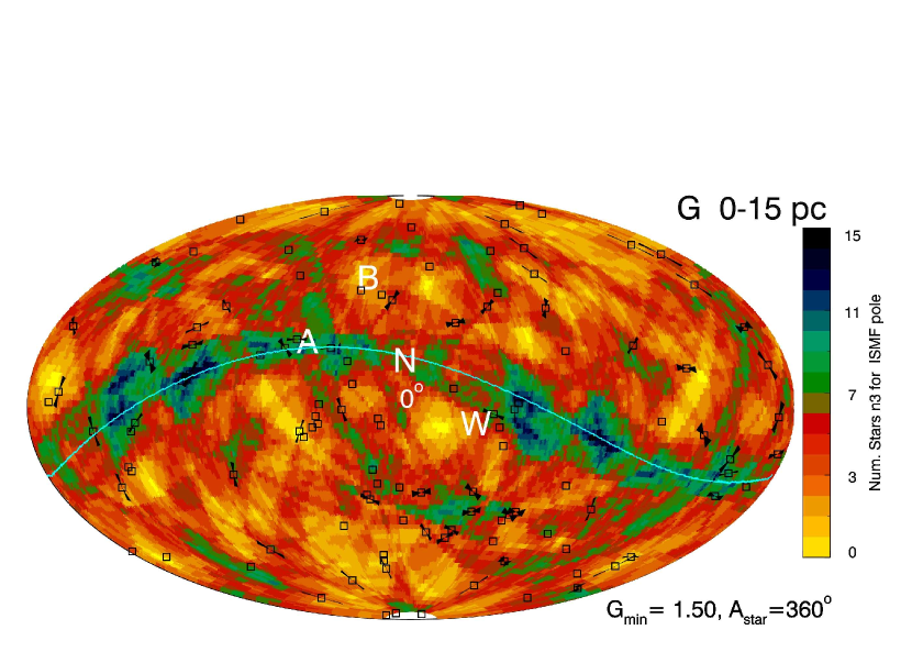
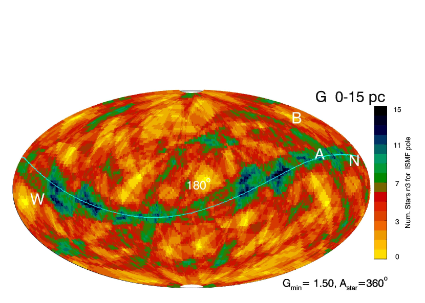
Figure 4: Magnetic structure traced by polarization data within 15 pc are shown by counting the number of polarization position angles that predict a “true” magnetic field directed toward each position on the sky. The probability at each location, $\Gamma$(L_rot,B_rot)  is evaluated for stars throughout the sky ($\alpha_{\mathrm{max}}$$=360^{\circ}$), and those with an ISMF located at $\theta_{\mathrm{rot}}$ values that satisfy $\Gamma$(L_rot,B_rot)$>$$\Gamma_{\mathrm{min}}$=1.0 (top) or $\Gamma$(L_rot,B_rot)$>$$\Gamma_{\mathrm{min}}$=1.5 (bottom) are included in the counts plotted on the maps. The cyan-colored line corresponds to the polarization band that has an axis toward $\ell$,$b$= 214^∘, 67^∘. The black angular symbols show polarization position angles where $P$/$dP$$>1.9$, while the squares show stars where $P$/$dP$$<1.9$. The letters “N”, “B”, “W”, and “A” indicate the directions of the heliosphere nose corresponding to the inflowing interstellar wind direction, the magnetic field direction indicated by the IBEX ribbon center, the upwind direction of the CLIC in the LSR, and the direction of the solar apex motion. Raising the minimum probability $\Gamma_{\mathrm{min}}$ used for selecting data included in the map decreases the total numbers of counts in the map and alters the color scale. Projections are centered on the galatic center (left) and anti-center (right), with galactic longitude increasing from right to left for the Aitoff projections plotted in this paper.

The extended polarization data base for stars within 40 pc is used to display the data that trace the IBEX interstellar magnetic field orientation according to the statistical criteria. Figure 3 gives an example of statistically combining polarization position angle probability swaths that produce the magnetic structure obtained in the direction of the center of the IBEX ribbon. The plotted probability swaths are those intersecting in the region outlined by the cyan-colored polygon in Figure 3. No angular restrictions are placed on the locations of the stars counted at each value of $L_{\mathrm{rot}}$, $B_{\mathrm{rot}}$ in these two figures, where $\alpha_{\mathrm{max}}$=360^∘, so that normalization is not needed. Rotated polarization position angles, $\theta_{\mathrm{rot}}$, have probabilities $\Gamma$(L_rot,B_rot)$>$$\Gamma_{\mathrm{min}}$ larger than $\Gamma_{\mathrm{min}}$=0.6 (left), or $\Gamma_{\mathrm{min}}$=0.9 (right), for tracing a magnetic field orientation inside the box. The color coding is dynamically generated for each map so that the small increase in $\Gamma_{\mathrm{min}}$ between maps modifies the color scheme and tends to give the appearance of more tightly defined spatial regions with higher probability data points. The color-bars in Figures 3 and 4 give the total number of stars counted into each location according to the statistical criteria. The polarization position angles of the contributing data points are plotted using black symbols, and the variations in uncertainties for the diverse data sample is shown by the variations in the angular uncertainties representing $\delta\theta_{\mathrm{PA}}$.

Comparisons between Figures 3 right and left show that the lower probability data points trace more extended regions defined by weaker statistical constraints. Note that the color-bar nomenclature in Figure 3 and other maps may include the annotations “n0”, “n1’, “n2” or “n3’. The value “n0” indicates that probabilities less than a $\Gamma_{\mathrm{max}}$ are plotted. Values “n1’, “n2” or “n3” indicate, respectively, that $\Gamma_{\mathrm{min}}$ displayed on the figure is n=1, n=2, or n=3 times an assumed baseline probability ($\Gamma_{\mathrm{min}}$/n). The values of the map constraints $\Gamma_{\mathrm{max}}$ and $\Gamma_{\mathrm{min}}$ are arbitrarily selected to provide maps with enough counts to be useful for color coding, and are shown on the figures. Smaller $\Gamma_{\mathrm{min}}$ values produce more extended high-count regions, while larger $\Gamma_{\mathrm{min}}$ values sharpen the magnetic structure, have lower counts, and may lead to inadequate sampling of spatial structure. The practical impacts of varying $\Gamma_{\mathrm{min}}$ and $\Gamma_{\mathrm{max}}$ is to change the color-coding in the figure and the visual impact of the color-coded magnetic pattern (Figure 3).

Identifying locations with small or large counts of data that meet the statistical criterion for tracing true magnetic field directions provides a diagnostic of magnetic structure that can be applied over all spatial scales if an adequate sample of data is available. Considerations when constructing maps from polarization data are that small values of $P$/$dP$ may indicate the lack of foreground dust, the absence of a magnetic field, and/or a strongly depolarizing foreground screen. Polarization data alone do not distinguish between these possibilities. This approach is free from prior assumptions about the physical configuration or origin of the magnetic fields that align the dust grains aside from the assumption that position angles are parallel to the intervening interstellar magnetic field orientation.

For any location $L_{\mathrm{rot}}$, $B_{\mathrm{rot}}$, the number of polarizations that trace a “true” magnetic field orientation tends to be less than the number of polarizations that do not trace a magnetic field orientation, so that generally more data are included in the maps constructed with the criterion $\Gamma$(L_rot,B_rot)$<$$\Gamma_{\mathrm{max}}$ than for maps constructed for $\Gamma$(L_rot,B_rot)$>$$\Gamma_{\mathrm{min}}$ (Figure 2).

The construction of maps with enough counts to be useful requires angular smoothing of the data. Smoothing over large angles masks small scale structure but highlights large-scale features. Smoothing is accomplished by allowing all stars within angle $\alpha_{\mathrm{max}}$ (degrees) of $L_{\mathrm{rot}}$, $B_{\mathrm{rot}}$ to contribute to the counts. Maps displaying angular smoothing over hemispheres ($\alpha_{\mathrm{max}}$=90^∘, §3.2) and smaller scales ($\alpha_{\mathrm{max}}$=60^∘, $\alpha_{\mathrm{max}}$=45^∘,§3.3) are shown. Values of $\Gamma_{\mathrm{min}}$ and $\Gamma_{\mathrm{max}}$ are selected so that a sufficient number of stars are mapped to provide useful color coding of magnetic structure and are responsive to the numbers of counted points that increase with larger angular sampling intervals.

3.1 Globally Smoothed Magnetic Structure and Polarization Band ($\alpha_{\mathrm{max}}$=360^∘)

The probability that a polarization position angle traces a true magnetic field orientation is the parameter used in this study to map the structure of the ISMF within 15 pc. The first stage of the analysis is to assume that the interstellar magnetic field is uniform in the nearest 15 pc, using $\alpha_{\mathrm{max}}$=360^∘, so that stars throughout the sky are included in the mapping of overlapping position angle swaths at each location. Rotated position angle, $\theta_{\mathrm{rot}}$, values are selected to satisfy the criterion $\Gamma$(L_rot,B_rot)$>$$\Gamma_{\mathrm{min}}$=1.0 (Figure 4, top) or $\Gamma$(L_rot,B_rot)$>$$\Gamma_{\mathrm{min}}$=1.5 (Figure 4, bottom), as the criterion for tracing a true magnetic field oriented toward each $L_{\mathrm{rot}}$,$B_{\mathrm{rot}}$ grid point. An implicit property of the constraint $\alpha_{\mathrm{max}}$=360^∘ is that the resulting magnetic pattern will have mirror symmetry since each polarization position angle traces two locations in opposite directions on the sky. The labels on the color-bars in Figures 4 shows counts of the number of stars with $\Gamma$(L_rot,B_rot)$>$$\Gamma_{\mathrm{min}}$=1.0 (top), or $\Gamma$(L_rot,B_rot)$>$$\Gamma_{\mathrm{min}}$=1.5 (bottom) of Figure 4. The probability distributions in Appendix A suggest that $\Gamma$(L_rot,B_rot)$>$$\Gamma_{\mathrm{min}}$=1.0 will test values of $|\theta_{\mathrm{rot}}|$ that are typically smaller than $\sim 20^{\circ}$, although the limiting angle depends on $P$/$dP$ for each data point. The color-bar in Figure 4 is labeled with the counts of numbers of overlapping position angle swaths at each grid locations. Color coding levels vary between the maps. Polarization position angles of the stars contributing to the $\alpha_{\mathrm{max}}$=360^∘ maps are plotted with black symbols with triangular extensions showing the uncertainties $\pm$$\delta\theta_{\mathrm{PA}}$ projected onto the figures, and the maps are shown centered on the galactic center and anti-center.

The magnetic pattern in Figure 4 ($\alpha_{\mathrm{max}}$=360) is dominated by a prominent band where the magnetic field orientation is restricted to being quasi-parallel to the sightline by the statistical requirements $\Gamma$(L_rot,B_rot)$>$$\Gamma_{\mathrm{min}}$=1.0, top, and $\Gamma$(L_rot,B_rot)$>$$\Gamma_{\mathrm{min}}$=1.5, bottom. A great circle that provides a good approximation to the curvature of the polarization band feature has an axis toward galactic coordinates $\ell$=214^∘, $b$=67^∘ and is tilted by 23^∘ with respect to the plane of the Galaxy (see Table 1 for values in equatorial and ecliptic coordinate systems). The equator of the great circle tracing the polarization band is plotted with a cyan-colored line on most figures.

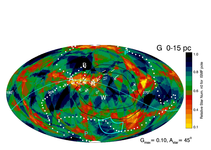
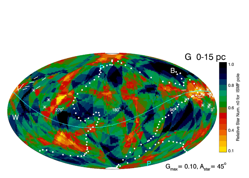
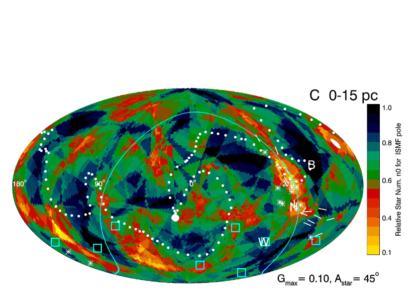
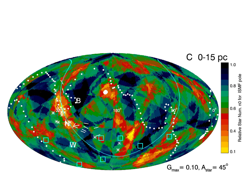
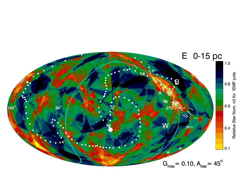
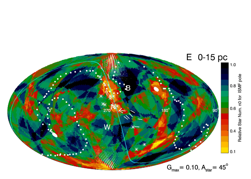
Figure 8: Same as Figure 7 except that the angular sampling is over intervals of $\alpha_{\mathrm{max}}$=45^∘.

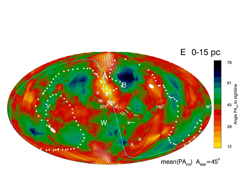
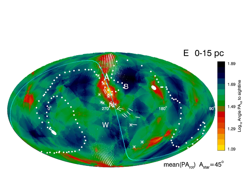
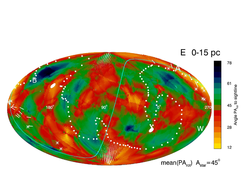
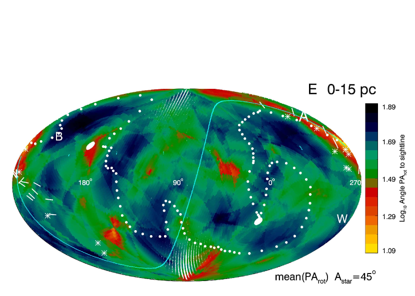
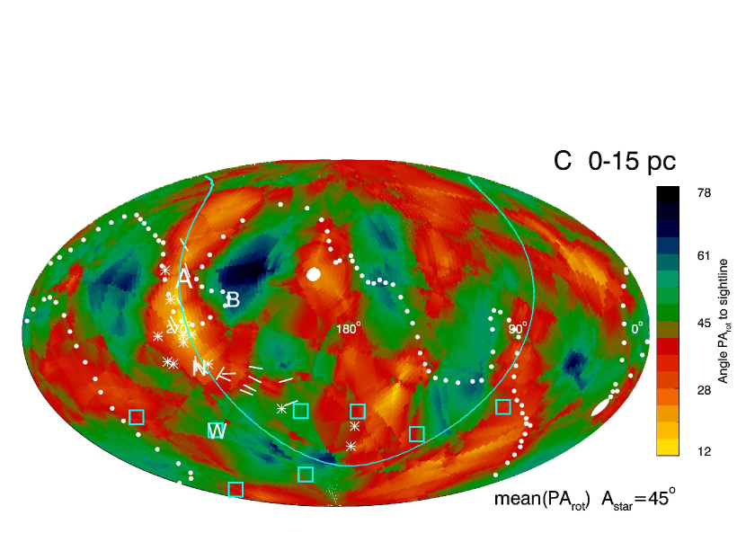
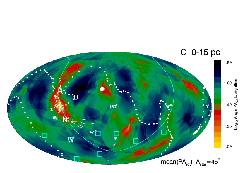
Figure 12: Same as Figure 11 except that projections are given in nose-centered and tail-centered ecliptic coordinates (left, top and middle), and equatorial coordinants centered on RA=12H.

The polarization band is defined by overlapping polarization position angle swaths and the axis of the great circle that corresponds to the polarization band configuration does not correspond to a magnetic pole direction (Appendix B). Instead, the polarization band overlaps the direction of the warm breeze flowing into the heliosphere (§6.4), and tends to separate the port and starboard sides of the heliosphere at lower latitudes (see the nose-centered ecliptic projections of Figures 8, 12).

The band is patchy and shows a gap of about 15^∘ on the galactic-west of the heliosphere nose starting at $\ell$$\sim 243^{\circ}$ and extending south to $\ell$$\sim 228^{\circ}$ (Figure 4). Such a gap is produced, for the mapping procedure used here, only if fewer magnetic field-lines overlap inside of the gap in comparison to adjacent regions (since the number of overlapping position angle swaths traces the number of overlapping magnetic field lines according to probability constraints). In the absence of prior knowledge about the true magnetic field direction that is being traced, it is not possible to distinguish between a true gap and unknown biases in the data underlying the analysis. The physical locations of the underlying stellar data set does not cause the gap (Appendix D). This gap is located close to the upwind direction of the flow of the CLIC through the LSR, and is labeled “W” for “wind” on the figures. The CLIC flows through the LSR away from the direction $\ell$=335^∘, $b$=$-$7^∘, with a velocity $-17$ ${\rm km~{}s}^{-1}$ (FRS11). Maps based on smaller $\alpha_{\mathrm{max}}$ values further constrain the gap (§3.3). Most locations with high counts of statistically qualifying position angles in the $\alpha_{\mathrm{max}}$=360^∘ maps are located in the polarization band feature (Figure 4).

3.2 Hemispheric Smoothing of Magnetic Structure ($\alpha_{\mathrm{max}}$=90^∘)

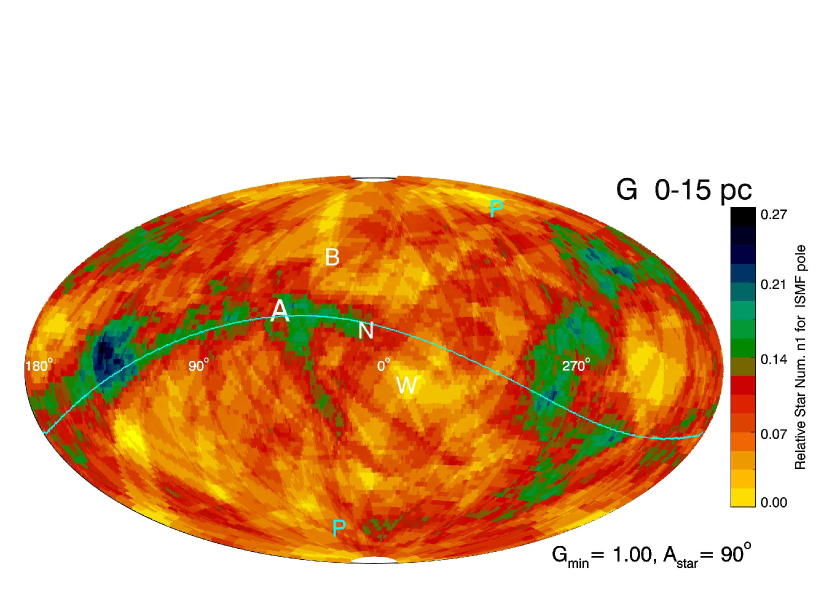
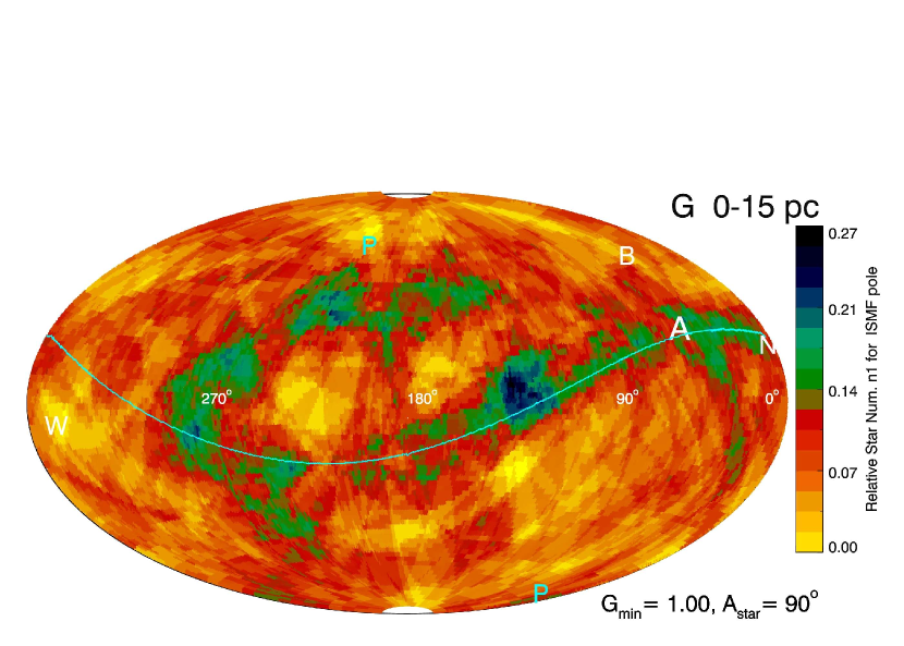
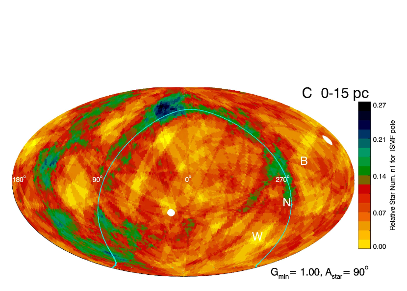
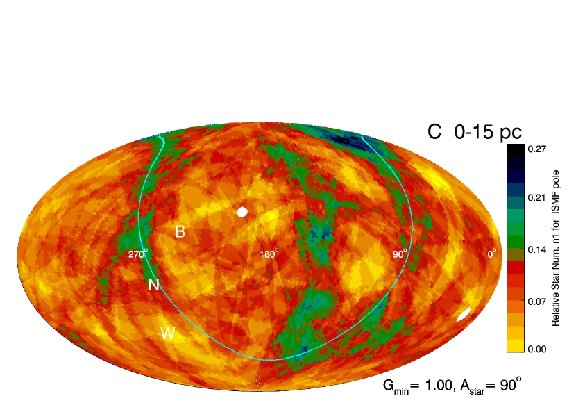
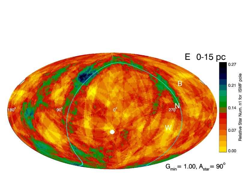
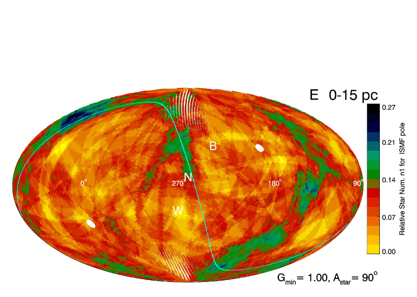
Figure 5: The relative numbers of stars with probability counting criteria $\Gamma$(L_rot,B_rot)$>$$\Gamma_{\mathrm{min}}$=1.00, and within 90^∘ of each grid point, are plotted. Plots are presented in galactic (’G’), equatorial (’C’) and ecliptic (’E’) coordinate systems. Top left and right figures are centered on galactic center and anti-center, respectively. Middle left and right figures are centered on 0^∘ and 180^∘ right ascension. Bottom left and right figures are centered on ecliptic coordinates $\lambda,\beta=0^{\circ},0^{\circ}$, left) and the heliosphere nose ($\lambda,\beta=255.6^{\circ},5.1^{\circ}$, right). Large white dots show the galactic poles. Other notations are as in Figure 4

Mapping counts of overlapping PPA swaths using $\alpha_{\mathrm{max}}$=90^∘ is equivalent to counting polarization position angles of stars located in the same hemisphere as the grid point $L_{\mathrm{rot}}$,$B_{\mathrm{rot}}$. For smoothing over subsections of the sky two criteria are used selecting stars that are counted into the figures, the statistical criterion and the angular criterion. The numbers of data points within $\alpha_{\mathrm{max}}$ degrees of a grid point ($L_{\mathrm{rot}}$, $B_{\mathrm{rot}}$) is more likely to vary across the maps for smaller smoothing angles because of the inhomogeneous distribution of the target stars on the sky. This possible differences in the number of data points found within $\alpha_{\mathrm{max}}$ of the $L_{\mathrm{rot}}$, $B_{\mathrm{rot}}$ grid locations can be compensated for by normalizing the number of statistically qualifying data points at each grid point with the total number of stars within $\alpha_{\mathrm{max}}$ of that grid point. The color-bar labeling in Figure 5 therefore is based on a scale of 0.0–1.0 (as are the later maps that are plotted with a linear color scale). The polarization band feature becomes most apparent in the first and second galactic quadrants ($\ell$=0^∘– 180^∘) and is patchy. The polarization band feature is asymmetric between Galactic quadrants I and II ($\ell$=0^∘– 180^∘) versus III and IV ($\ell$=180^∘– 360^∘) in the $\alpha_{\mathrm{max}}$=90^∘ map, and for this set of constraints is not evident for galactic $\ell$$>$180^∘, or equivalently the ecliptic south of the heliosphere nose.

Polarizations included in the angmax=90^∘ map have a relatively high probability, $\Gamma$(L_rot,B_rot)$>1.0$, of tracing an ISMF near the sightline but only 27% of the geometrically qualifying stars satisfy this statistical criteria as shown in Figure 5. The probability distributions in Appendix A suggest that probabilities larger than 1.0 typically correspond to $|\theta_{\mathrm{rot}}|$$<12^{\circ}$, and therefore trace magnetic fields oriented within $\sim 12^{\circ}$ of the plotted locations, although this value varies somewhat with $P$/$dP$ of the measurement. Based on this argument it appears the polarization band is formed of values of $|\theta_{\mathrm{rot}}|$ that are near the radial sightline.

The gap seen to the right of the heliosphere nose in the $\alpha_{\mathrm{max}}$=360^∘, $\Gamma$(L_rot,B_rot)$>1.00$ galactic projection enlarges to over 60^∘ wide in the $\alpha_{\mathrm{max}}$=90^∘ map. The gap is evident as large reddish regions with few stars tracing magnetic field orientations parallel to sightlines. This gap borders the upwind direction of the CLIC flow through the LSR (Table 1), marked by a ”W’ on figures. Figure 5, lower right. For the ecliptic projection centered on the heliosphere nose, the gap also coincides with the southern ecliptic latitudes below the heliosphere nose. This southern region overlaps the regions of highest magnetic pressures for heliosheath plasma according to IBEX ENA data (Schwadron et al., 2014b; McComas et al., 2017, Table 1).

3.3 Smoothing Magnetic Structure over Angular Scales of 60^∘ and 45^∘

Different magnetic field orientations can be selected through the probability constraints. For the data utilized here, the number of data points found to have small probabilities for tracing a magnetic field at a value of $L_{\mathrm{rot}}$,$B_{\mathrm{rot}}$ is typically greater than the number of data points with large probabilities for tracing a magnetic field at the location (Figure 2 and Appendix A). Smaller spatial sampling intervals can be used when larger numbers of stars qualify statistically for plotting.

Maps are constructed by binning probability distributions using two limits, those with $\Gamma$(L_rot,B_rot) larger or smaller than the limiting value. Maps constructed with the criterion $\Gamma$(L_rot,B_rot)$<0.63$ (§3.3.1) will count larger numbers of stars with magnetic fields favoring an field orientation near the plane of the sky than maps based on the criterion $\Gamma$(L_rot,B_rot)$<0.1$ (§3.3 because of the peaked probability distribution for $P$/$dP$$>1.9$ (Appendix A). Maps built with conditions $\Gamma$(L_rot,B_rot)$<$$\Gamma_{\mathrm{max}}$ are also restricted to data where $P$/$dP$$>1.9$ in order to avoid counting regions where no dust grains are present. Relative numbers of stars that have values $\Gamma$(L_rot,B_rot) larger (smaller) than the probability cutoffs $\Gamma_{\mathrm{min}}$($\Gamma_{\mathrm{max}}$), then become a diagnostic of the typical value of $|\theta_{\mathrm{rot}}|$ in each sightline. The goal is to obtain the best angular resolution that maximizes the statistical significance of the derived magnetic structure and also avoids spatial gaps not sampled by the available data. Smaller values of $\alpha_{\mathrm{max}}$ reduce the number of geometrically qualifying data points at each location. Generally, the numbers of data points traced at each location using the criteria $\Gamma$(L_rot,B_rot)$<$$\Gamma_{\mathrm{max}}$ tends to be larger than the numbers of data points with $\Gamma$(L_rot,B_rot)$>$$\Gamma_{\mathrm{min}}$ at the same location if $\Gamma_{\mathrm{min}}$=$\Gamma_{\mathrm{max}}$. The criteria $\Gamma$(L_rot,B_rot)$<$$\Gamma_{\mathrm{max}}$ therefore allows more spatial detail in the plotted magnetic structure. The limit $\Gamma$(L_rot,B_rot)$<$$\Gamma_{\mathrm{max}}$ emphasizes magnetic field directions with statistically low probabilities of tracing magnetic fields aligned with $L_{\mathrm{rot}}$, $B_{\mathrm{rot}}$ and there emphasizes field field orientations quasi-parallel to the plane of the sky. Fewer data points are counted generally with the limit $\Gamma$(L_rot,B_rot)$>$$\Gamma_{\mathrm{min}}$ (Appendix A). Smaller angular smoothing intervals enable comparisons between magnetic structure and interstellar and heliospheric phenomena that are sensitive to magnetic structure.

3.3.1 Emphasizing Fields Quasi-Parallel to Plane of Sky

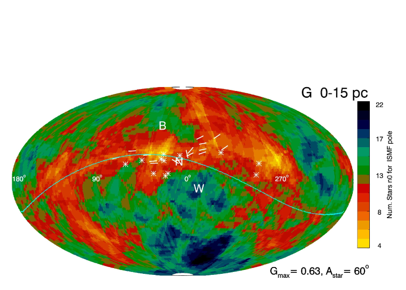
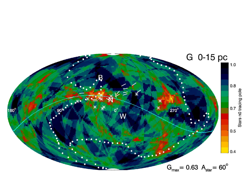
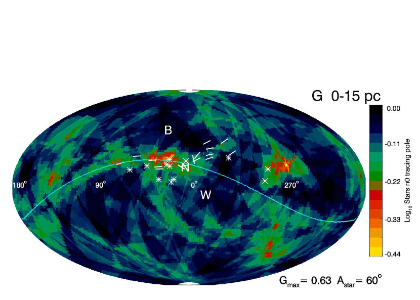
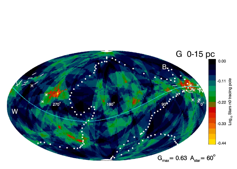
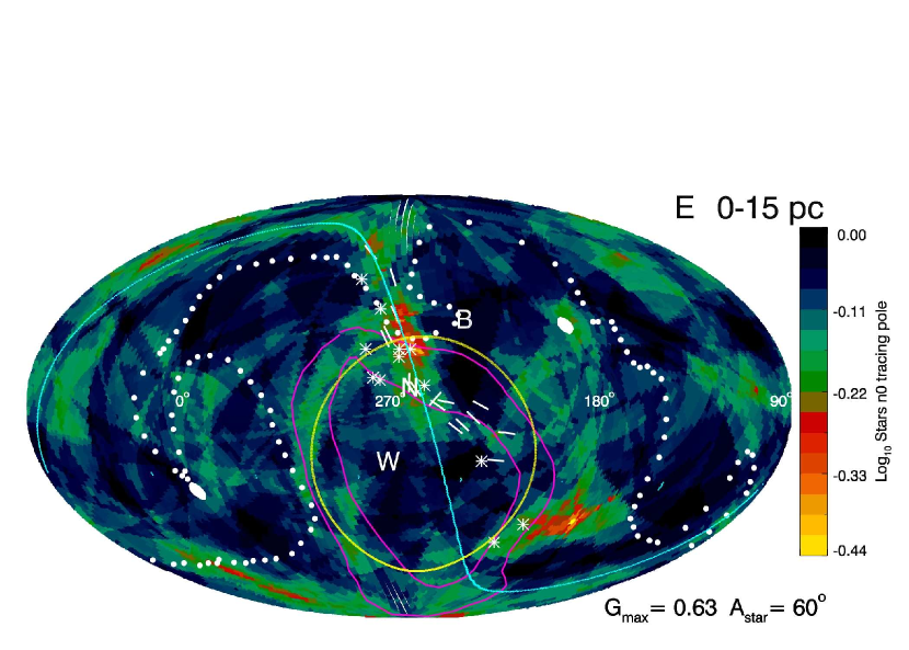
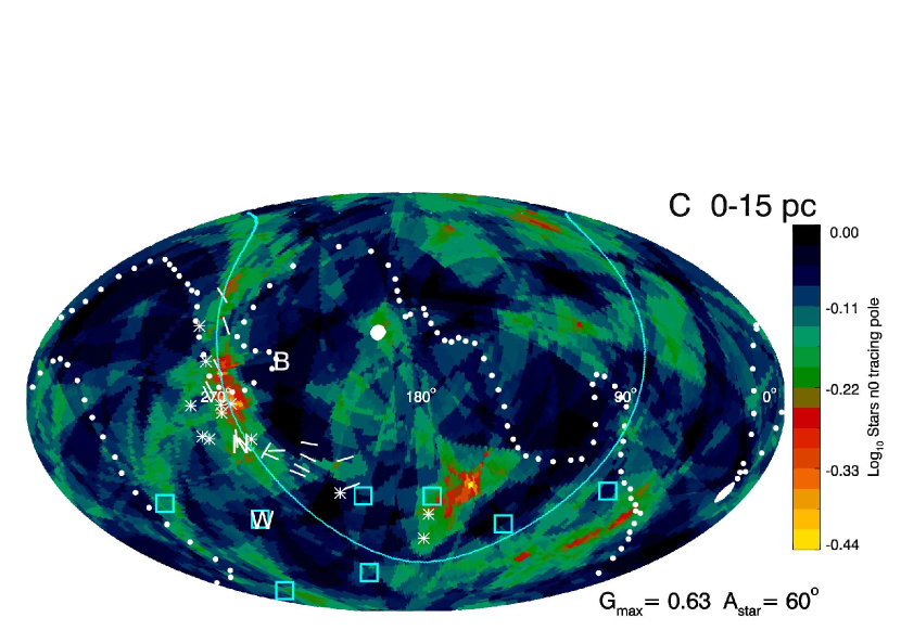
Figure 6: Maps of unnormalized (top left) and normalized counts (other figures) of data where $\Gamma$(L_rot,B_rot)$<$$\Gamma_{\mathrm{max}}$=0.63 that are within 60^∘ of each plotted location $L_{\mathrm{rot}}$, $B_{\mathrm{rot}}$, using data with Pol/$dP$$\geq 1.9$. Counts are normalized by the number of points within $\alpha_{\mathrm{max}}$=60^∘ of each point. The bottom four maps display results with a logarithmic color scale (base 10), for projections in the galactic, ecliptic, and equatorial coordinate systems (‘G”, “E”, and “C”). Supplementary data plotted include the kHz emissions discovered by Voyagers 1 and 2 (asterisks) and the filament star polarizations (bars). Concentric contours outline the Loop I shell. The white ring in the nose-centered ecliptic projection (lower left) shows the approximate region of high plasma pressures discovered by IBEX (centered near $\lambda$=249^∘, $\beta$=–20^∘). The gap in the polarization band corresponds to both the center of Loop I and the heliosheath high-pressure plasma region. Galactic cosmic ray small excess regions (IC59) are shown in the lower right figure (cyan-colored squares, §6.9).

Figure 6 shows the importance of normalization on the plotted magnetic structure and varies the data display to show the influence of the color scale on perceived magnetic structure. The unnormalized top left figure in Figure 6 has extended reddish regions with star counts of 10 or below. Variations in the total number of data points available at each location for the geometric criteria set by $\alpha_{\mathrm{max}}$ indicate that the more useful number of normalized statistically qualifying data points (top right, Figure 6) should be used. The top left figure counts about eight stars in the heliosphere nose region that statistically qualify to be counted as for the condition $\Gamma$(L_rot,B_rot)$<0.63$, which corresponds to a field orientation with respect to the sightline of $\theta_{\mathrm{rot}}$ larger than $>19$^∘ (Appendix A, the exact angle limit depends on $P$/$dP$). The top right figure shows that roughly 60% of the geometrically qualifying data points have $\Gamma$(L_rot,B_rot)$<$0.63, and the remaining 40% of the data trace an ISMF in the heliosphere nose region with $\theta_{\mathrm{rot}}$$<19$^∘, and field lines quasi-parallel to sightlines. Normalization of the number of stars meeting the statistical constraint by the total number of stars meeting the geometric constraint therefore yields a more accurate description of magnetic structure by avoiding map patterns dominated by the distribution of the stars. Counts of stars in the data base that are within 60^∘ of each position $L_{\mathrm{rot}}$, $B_{\mathrm{rot}}$, for data with $P$/$dP$$>1.9$, are shown in Appendix D. There is no relation between the derived magnetic structure in this paper and the spatial distribution of the stars.

Color contrasts differ if a logarithmic color scale (to base 10) is used, as seen in the middle and lower images of Figure 6. These figures also display supplementary data for phenomena that are sensitive to local interstellar or heliosphere magnetic field structure, overlaid on galactic, ecliptic and equatorial projections. The normalized figures displayed with a logarithmic color scale give different color contrasts that emphasize different physical structures in the data.

Loop I is plotted with concentric lines in Figure 6. An elongated green polarization filamentary feature is present on the east side of the southern part of Loop I, extending between $\ell$,$b$$\sim 30^{\circ},0^{\circ}$ to $\ell$,$b$$\sim 0^{\circ},-35^{\circ}$ (east of the heliosphere nose for the plot in ecliptic coordinates). This polarization filament extends to within 15 pc of the heliosphere and could alternatively be associated with an extension of the Loop I superbubble to the solar location. Interior to Loop I magnetic field orientations that are quasi-parallel to the sightlines are avoided (Figure 6, middle left).

An alternative picture places this same green filament on the east side of the region of highest heliosheath pressure found by IBEX (McComas & Schwadron, 2014). The green circle in the lower right panel in Figure 6 is centered south of the ecliptic nose at ecliptic coordinates $\lambda$=249^∘, $\beta$=–20^∘, with a radius of 47^∘, corresponding to the central regions of highest heliosheath pressures. The interior of Loop I and the region of highest heliosheath pressure can not be distinguished geometrically in the plane of the sky, most likely because Loop I has expanded to the solar location, dominates the CLIC configuration, and dominates the CLIC and LIC kinematics (see reviews FRS11, Frisch & Dwarkadas, 2018).

Maps are displayed in galactic, equatorial, and ecliptic coordinate systems to allow comparison with other data sets.

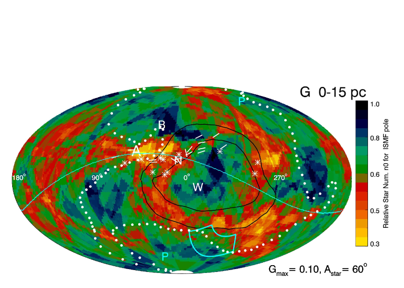
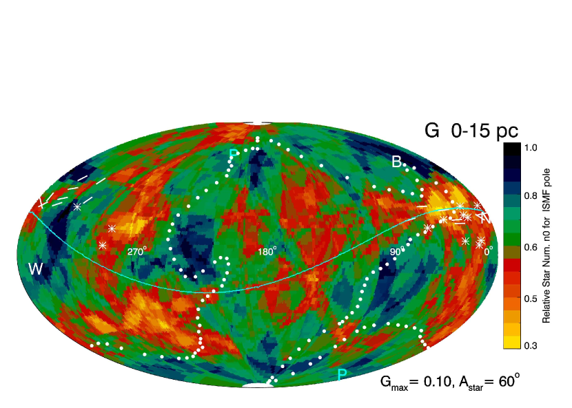
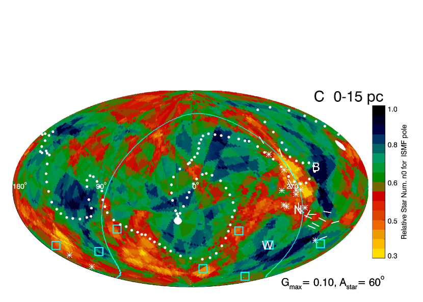
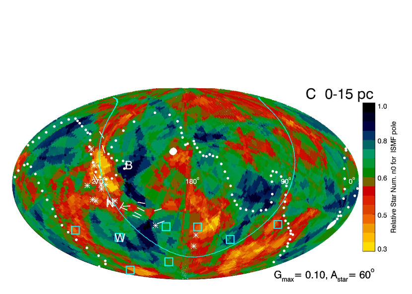
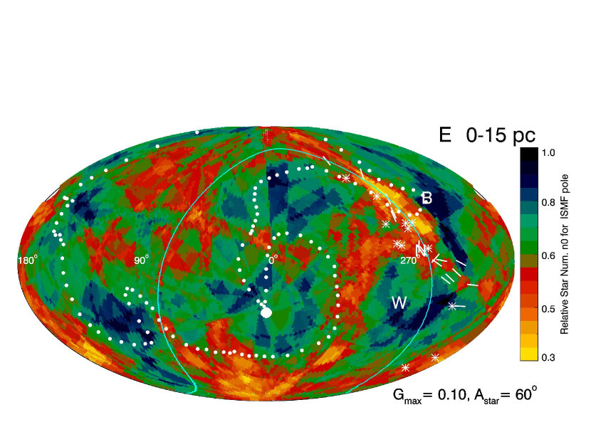
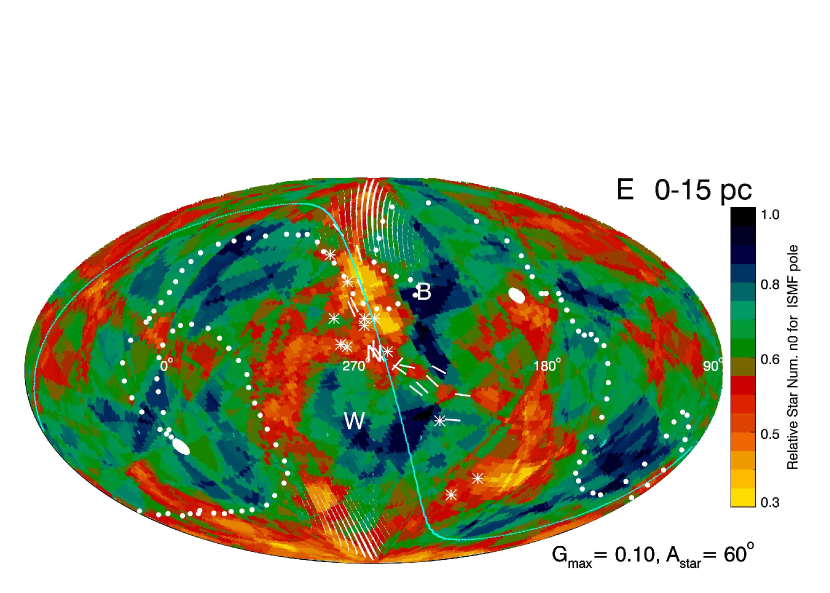
Figure 7: The three figure pairs show magnetic structure for statistical constraints $\Gamma$(L_rot,B_rot)$<$$\Gamma_{\mathrm{max}}$=0.10 and angular sampling over intervals $\pm 60^{\circ}$ ($\alpha_{\mathrm{max}}$=60^∘) around each grid point. Numbers of statistically qualifying data points are normalized by the numbers of geometrically qualifying data points at each location. Other features in figures are explained in Figure 6.

Several external data sets that are sensitive to local magnetic phenomena are plotted in Figures 6–8 and discussed in Section 6. These data include the contours that outline the Loop I configuration defined by polarization data (Santos et al., 2011), low frequency radio emissions measured by by Voyager 1 and Voyager 2 that originate as plasma emissions in the interstellar gas upwind of the heliopause (Kurth & Gurnett, 2003; Gurnett et al., 2013), the polarizations of a dust filament around the heliosphere (Frisch et al., 2015a), and the ICECUBE59 cosmic ray point sources.

3.3.2 Emphasizing Fields Quasi-Parallel to Sightlines

Broad regions are found in nearby space where magnetic fields tend to be oriented closer to the sightlines than to the plane of the sky. A consistent picture is obtained for the polarization band magnetic structure in the first two Galactic quadrants, $\ell$=0^∘–180^∘, based on the maps with lower limits imposed on $\Gamma_{\mathrm{min}}$, $\Gamma$(L_rot,B_rot)$>$$\Gamma_{\mathrm{min}}$ (Figures 4, 5). The polarization band is a semi-continuous feature in these maps. The more restrictive constraint of $\Gamma$(L_rot,B_rot)$<$$\Gamma_{\mathrm{min}}$=0.1 in Figure 7 ($\alpha_{\mathrm{max}}$=60^∘) and Figure 8 ($\alpha_{\mathrm{max}}$=45^∘) selects out the stars for plotting that have $\theta_{\mathrm{rot}}$$>37^{\circ}$ so the position angles are not aligned with the sightline. The result is a patchy magnetic structure that discriminates between data points on the shoulders of the probability distributions (Appendix A) along the great circle of the polarization band. In Figure 7 the polarization band great circle is visible as reddish regions (small counts of $\Gamma$(L_rot,B_rot)$<$0.1 and $\theta_{\mathrm{rot}}$$>$37^∘data points) in Galactic intervals 0^∘–90^∘, and as the border of greenish regions in galactic intervals 180^∘–270^∘. The difference between maps made with $\Gamma$(L_rot,B_rot)$<$$\Gamma_{\mathrm{max}}$=0.63 (Figure 6) and maps made with $\Gamma$(L_rot,B_rot)$<$$\Gamma_{\mathrm{max}}$=0.1 (Figures 7, 8) is that the $\Gamma$(L_rot,B_rot)$<$$\Gamma_{\mathrm{max}}$=0.1 constraint counts stars with $\theta_{\mathrm{rot}}$$\sim 19^{\circ}--37^{\circ}$ that are not included in the $\Gamma$(L_rot,B_rot)$<$$\Gamma_{\mathrm{max}}$=0.63 counts (again with details sensitive to values of$P$/$dP$). Regions where there are few or no stars with $\Gamma$(L_rot,B_rot)$<0.1$ (reddish regions of low counts in Figure 7) will be highlighting sightlines where the ISMF makes angles typically less than $\sim 37^{\circ}$ with respect to the sightline. For maps constructed with $\Gamma$(L_rot,B_rot)$<0.63$ the reddish regions correspond typically to stars with $\theta_{\mathrm{rot}}$ within $\sim 19^{\circ}$ of the sightline. These general characteristics of the statistical distributions suggest that the differences between mapped values in Figures 6 and 7 may be attributed to magnetic field orientations with respect to the sightline of $\theta_{\mathrm{rot}}$$\sim$19^∘–37^∘, which are counted in Figure 6, but not counted for $\Gamma_{\mathrm{max}}$=0.1 (Figure 7) Evidently the magnetic field along the polarization band has a tendency to rotate roughly 20^∘–40^∘ away from the sightline in parts of the second Galactic quadrant. This result is consistent with the mean polarization position angles plotted in §5.

4 Least-squares Analysis of the Best-fitting Magnetic Pole

Mapping overlapping polarization position angle swaths gives qualitative but not quantitative results on the direction of the magnetic field. An important symmetry of the polarization band data will be given by the direction of the dipole component of the magnetic field. The best-fitting magnetic pole to a set of position angle data can be found by performing a least-squares fit to sine($\theta_{\mathrm{PA}}$). We find below that the dominant dipole component of the magnetic fields for two well-defined subsets of these polarization data, the polarization band (§4.1) and the filament stars (§4.2), reflect the geometry of the heliosphere rather than the local interstellar gas.

A two-parameter least-squares fit is performed on position angles for subsets of the data in order to determine the most probable location for the magnetic pole sampled by these data. The dipole component of the magnetic field, toward $\ell_{\mathrm{pole}}$,$b_{\mathrm{pole}}$, can be found by minimizing the sum of the weighted values of sin($\theta_{\mathrm{PA}}$) for the stars. Data points are weighted using values of $P$/$dP$, rather than values of ($P$/$dP$)², in order to minimize biases introduced by the heterogeneous underlying data sample where $P$/$dP$ varies systematically between sets of data. In addition, $P$/$dP$ is capped at $P$/$dP$$<$6 to minimize biases from possible unrecognized intrinsic stellar polarizations.

The expected value for the sine of each polarization position angle $PA_{\mathrm{i}}$  is zero so the chi-squared variance ($var_{\mathrm{i}}$) of each measurement i is sin($PA_{\mathrm{i}}$ ) for N data points. The least-squares estimate of the sky position of the magnetic field will be at the location $\ell_{\mathrm{pole}}$, $b_{\mathrm{pole}}$ given by the minimum of the variance of the data points:

$$S_{\ell,b}=\frac{N}{N-2}{\Sigma_{\mathrm{i}}}\frac{w_{\mathrm{i}}(sin(PA_{\mathrm{i,obs}})-sin(PA_{\mathrm{i,\ell,b}}))^{2}}{w_{\mathrm{i}}}.$$ (1)

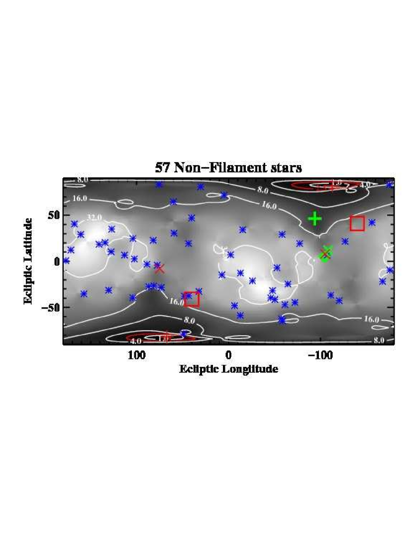
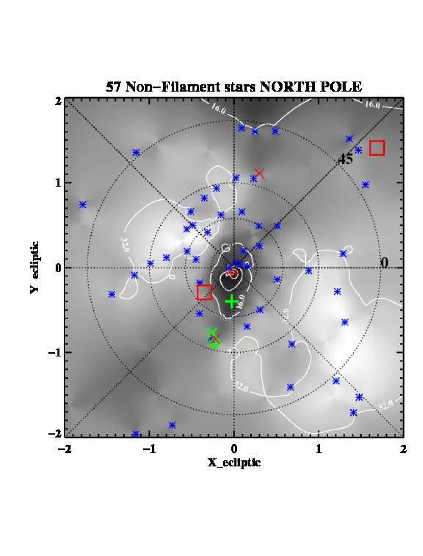
Figure 9: Gray-scale image showing the $\chi^{2}~{}$probabilities that the best 57 stars creating the polarization band will trace a magnetic field at each location in the ecliptic, for a linear (left) and a stereographic projection centered on the north ecliptic pole (right). The magnetic field direction traced by the polarization band (red “X”) overlaps the north ecliptic pole (Table 1). Blue asterisks show the locations of the 57 stars, tracing magnetic field directions within 10^∘ of the polarization band, used in this analysis. Red squares show the opposite poles of the IBEX ribbon magnetic field. Red plus symbols indicate locations of the poles of the dipole component of the magnetic field direction that is traced by the polarization band stars. Red “Xs” show the heliosphere nose and it’s opposite direction. The locations of the stars used to obtain these results are plotted with blue asterisks. The green diamonds, “X” and cross show the heliosphere nose location as defined by the interstellar He^∘ wind, the warm breeze flowing into the heliosphere, and the ISMF direction found from polarization data in Frisch et al. (2012). The red boxes indicates the ISMF direction from the IBEX ribbon and its opposite.

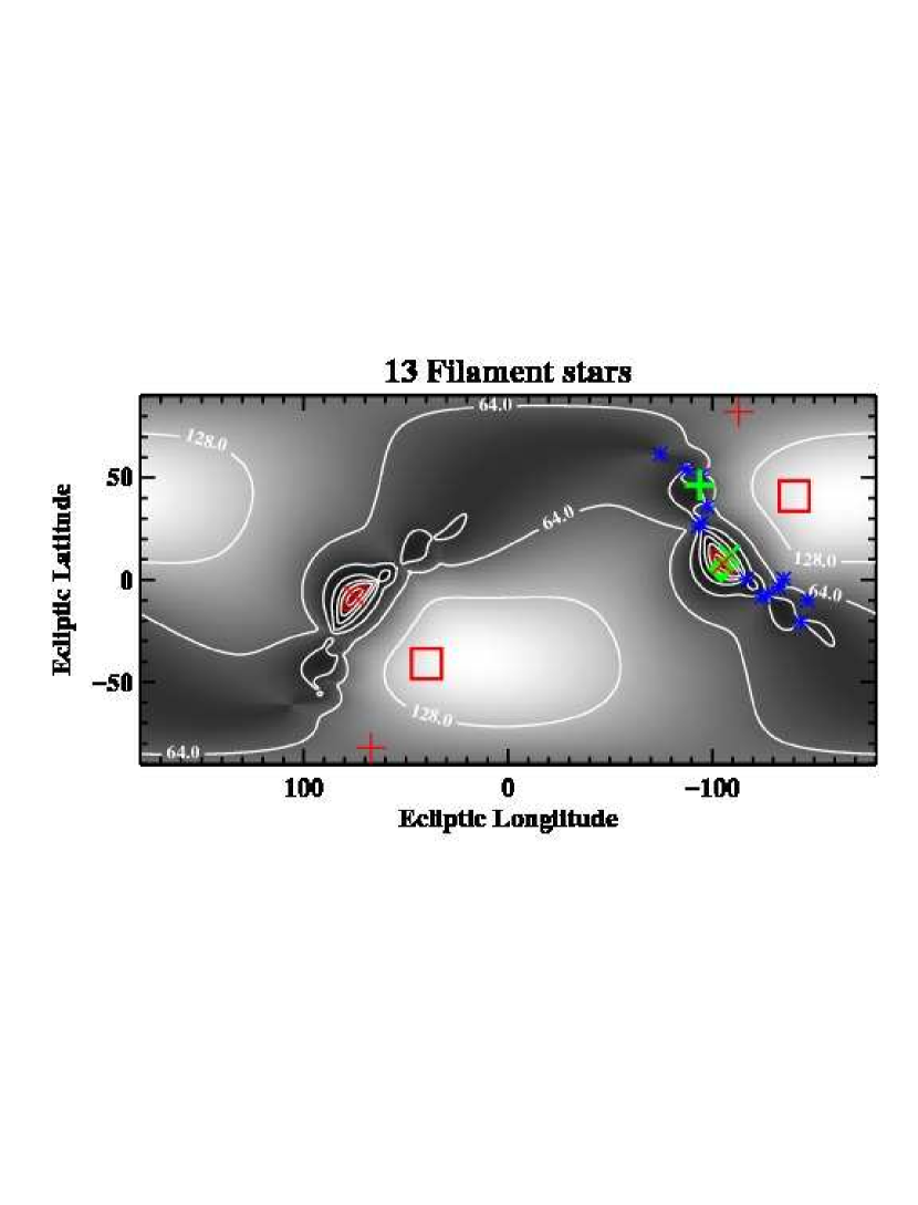
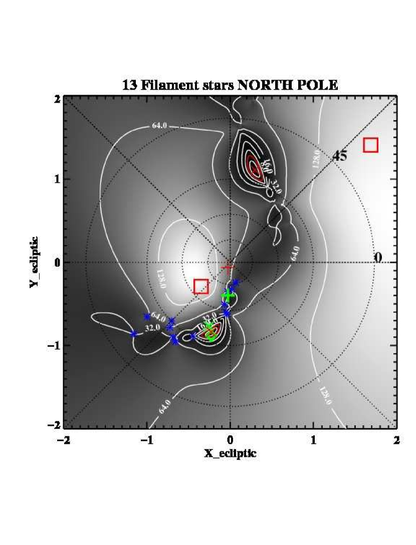
Figure 10: Results of a $\chi^{2}~{}$analysis of the best-fitting magnetic pole to the 13 filament stars are plotted in a gray scale with contour values showing $\Delta\chi^{2}$. The red contour shows $\chi^{2}~{}$=2.3, within which the magnetic pole has a 68% of being located. The Figures are plotted in ecliptic coordinates centered on $\lambda$,$\beta$=0^∘,0^∘ for a linear projection (left), and for a stereo projection centered on the north pole (right). The low probability zones outlined by $\chi^{2}~{}$=128.0, where filament stars show no evidence of tracing a magnetic field, are located approximately downwind of the heliosphere nose. The red “X” symbols shows the opposite locations of the two magnetic poles for the filament stars. See Figure 9 for explanation of other symbols.

The location $\ell_{\mathrm{pole}}$, $b_{\mathrm{pole}}$ of the minimum in $S_{\ell,b}$ is determined by constructing a grid on the sky of 360x180 points (the $L_{\mathrm{rot}}$, $B_{\mathrm{rot}}$ grid) and evaluating $S_{\ell,b}$ at each location on the grid. Contours of $\chi^{2}~{}$are evaluated and plotted for the polarization band stars (§4.1) and the filament stars (§4.2), using a red contour to indicate standard uncertainties that are 68.3% probable where $\chi^{2}=$ 2.30 (Figures 9 and 10).

4.1 Quantitative Analysis of the Polarization Band

The polarization band feature shown in Figures 4 and 5 arises from a locus of points in the sky where the interstellar magnetic field has a relatively high probability of being parallel to the sightlines. A subset of data that best traces the polarization band feature is selected to include stars with probabilities $\Gamma$(L_rot,B_rot)$>1.5$ for tracing an interstellar magnetic field orientation that is within 10^∘ of the polarization band (i.e. as given by the equator of a sphere with a pole located at the axis of the polarization band, §3.1, Table 1). Stars that trace the filament of polarizing dust grains around the heliosphere (Frisch et al., 2015a) are excluded from this subset since those polarization position angles are expected to have a different origin than that of the polarization band. Fifty-seven non-filament stars are found to have probabilities $\Gamma$(L_rot,B_rot)$>1.5$ for tracing a magnetic field pole within 10^∘ of the polarization band equator. Note that the filament stars were not excluded when the polarization band feature was first identified in Figure 4, but are excluded here where the origin of the polarization band is tested. The data for these 57 stars include polarization data collected during the 20th century (25 stars) and data collected in the 21st century. The diversity of data sources indicates that instrumental biases are unlikely to dominate the properties of the polarization band. The polarization band defined by these 57 stars then provides the basis for a least-squares analysis to determine the best-fitting magnetic field orientation to the polarization band.

A two-parameter least-squares fit was performed to the polarization position angles of these 57 stars to determine the most probable values of the interstellar magnetic pole sampled by these data. The location of the minimum in $S_{\ell,b}$ (equation 1) is at ecliptic coordinates $\ell,\beta=247^{\circ},~{}82.2^{\circ}(\pm 4.5^{\circ})$, for the $\chi^{2}=$ 2.3 fit (red contours, Figure 9), indicating that the best-fitting magnetic pole to the 57-star polarization band is within 7.8^∘ of the ecliptic poles (Table 1 gives values for galactic and equatorial coordinate systems). Figure 9 shows the $\chi^{2}~{}$contours of likelihood that a magnetic pole is found at each location for the 57 stars, in a linear (left) and a stereographic projection that is centered on the north ecliptic pole (right). The equator of the polarization band feature, with respect to the axis of the polarization band (Table 1), is based on a larger sample of stars that includes the filament stars and is 17.6^∘ away from the ecliptic poles at the position of closest approach. The polar location of the best-fitting magnetic pole to the 57-star sample of the polarization band suggests strongly that the dust grains are aligned with respect to the ISMF that is distorted by interactions with the heliosphere.

4.2 Quantitative Fit to Filament Stars

A quantitative least-squares fit was performed to the polarization position angles of the 13 filament stars originally identified in Frisch et al. (2015b). The best-fitting magnetic field orientation found from the least-squares analysis of these filament stars is toward $\ell$$=5.9^{\circ}\pm 8.2^{\circ}$, $b$$=17.0^{\circ}\pm 3.5^{\circ}$, a result consistent with the earlier value (Frisch et al., 2015a). Table 1 gives the filament magnetic pole in ecliptic coordinates. Figure 10 shows the $\chi^{2}~{}$contours for the filament stars in ecliptic coordinates, centered on the ecliptic nose (left) and in a stereographic projection centered on the north ecliptic pole (right). The red contour shows the $\chi^{2}=$ 68.3% probability contour.

5 Mapping Magnetic Field Mean Position Angles

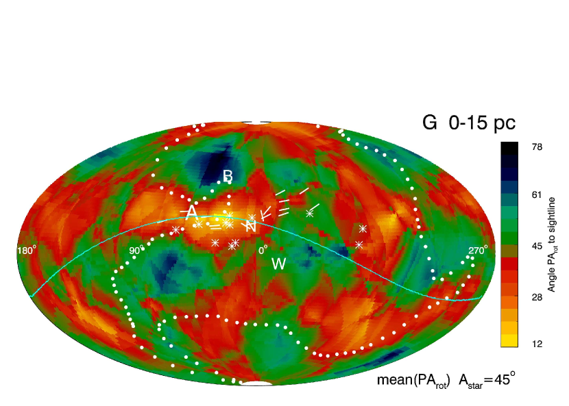
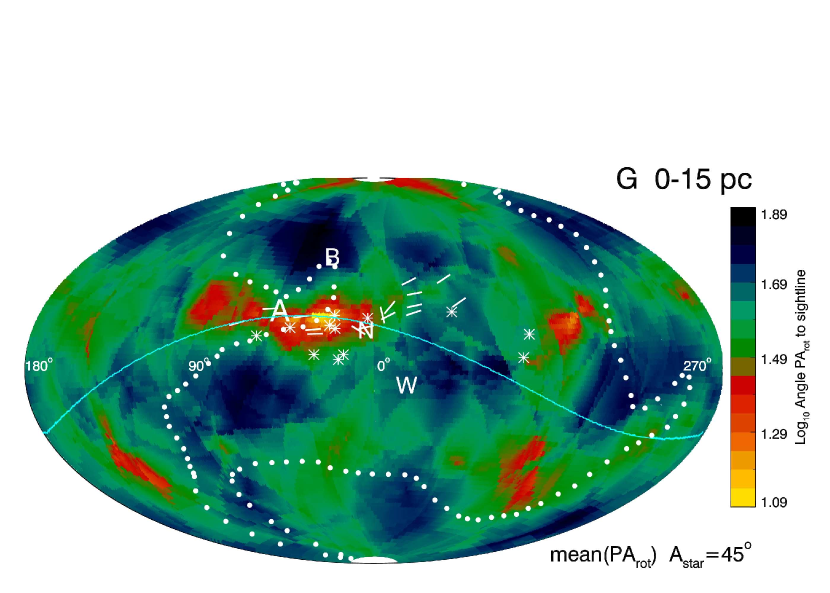
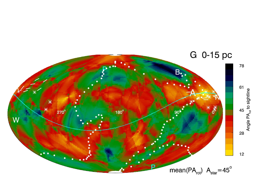
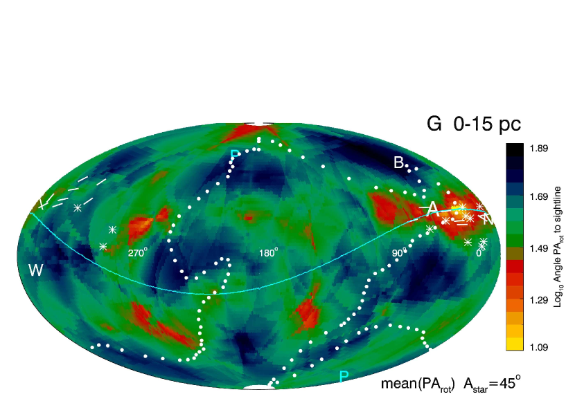
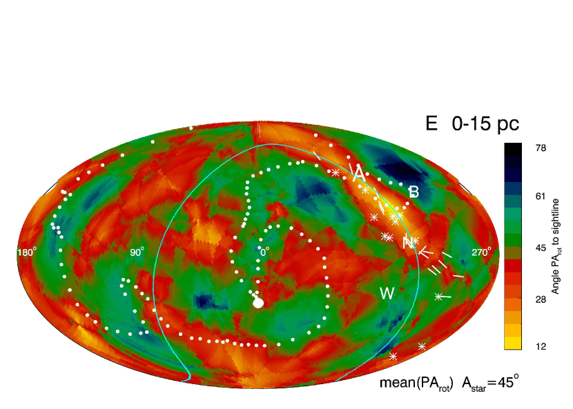
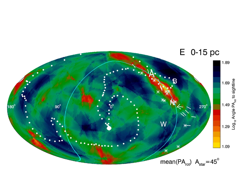
Figure 11: Mean values of $\theta_{\mathrm{rot}}$ at at each grid location $L_{\mathrm{rot}}$, $B_{\mathrm{rot}}$ are color-coded and plotted based on smoothing radius of 45^∘ ($\alpha_{\mathrm{max}}$=45^∘). Figures in the left column are plotted on a linear color scale and figures on the right column are plotted on a logarithmic color scale (base 10). Maps are displayed in galactic coordinates centered on the galactic center (top), anti-center (middle), and in ecliptic coordinates centered on 0^∘ (bottom). See Figure 12 for additional projections.

The methodology described in §3 is analogous to mapping values of $\theta_{\mathrm{rot}}$ according to preset probability bins. An alternate display of magnetic field structure relies on plotting mean values of $\theta_{\mathrm{rot}}$ at each location $L_{\mathrm{rot}}$, $B_{\mathrm{rot}}$ without imposing constraints on the probability $\Gamma$(L_rot,B_rot). Direct mapping of $\theta_{\mathrm{rot}}$ is useful only if the mapped data are required to have measurable polarization signal so data are also required to have $P$/$dP$$>1.9$ for inclusion in figures mapping $\theta_{\mathrm{rot}}$. Figures 11 and 12 show the mean values of $\theta_{\mathrm{rot}}$ for each location for a sampling radius of $\pm$45^∘. Maps are displayed in linear (left columns) and logarithmic (base 10, right columns) color scales. Figure 11, top right, where mean position angles are plotted on a logarithmic color scale, shows that the heliosphere nose region and the polarization band in the first galactic quadrant are dominated by $\theta_{\mathrm{rot}}$$\sim 25^{\circ}-30^{\circ}$ or less. The high-pressure region south of the ecliptic nose is seen in Figure 12 to be dominated by mean polarization position angles of $\theta_{\mathrm{rot}}$$>$50^∘. The large values for $\theta_{\mathrm{rot}}$ in this region are expected if these polarizations are influenced by the draping of the interstellar magnetic field over the heliosphere, since this is the region of maximum magnetic pressure according to models of the heliosphere (Pogorelov et al., 2011) and where the IBEX ENA ribbon forms (Zirnstein et al., 2016). The direction of the interstellar magnetic field traced by the IBEX ribbon, marked by the “B”, is in a region where $\theta_{\mathrm{rot}}$ varies spatially and tends to be $\theta_{\mathrm{rot}}$$>$50^∘. However the smoothing radius for these figures is $\pm 45^{\circ}$ so the plotted mean $\theta_{\mathrm{rot}}$ should not be expected to aligned directly with the magnetic field direction if the field orientation spatially varies as expected during the interaction with the heliosphere. The heliosphere nose region clearly stands out as a region where the magnetic field is quasi-parallel to sightlines.

6 Discussion

The patterns of the interstellar magnetic field found for stars within 15 pc show strong geometric symmetries related to the interaction between dust-bearing interstellar magnetic fields and the heliosphere, and extended patterns of field directions with angles larger or smaller than $\sim 19^{\circ}-37^{\circ}$ with respect to sightlines (depending on probability selection criteria). These extended patterns may trace either purely interstellar field directions or the interaction between the interstellar magnetic field and the heliosphere.

6.1 Polarization Band

The most unexpected feature in this study is the polarization band created by the overlapping position angle swaths (Figures 1, 4). The band was identified in an unbiased plot of all data that had probabilities larger than $\Gamma_{\mathrm{min}}$=1.5 for tracing an ISMF direction toward the $L_{\mathrm{rot}}$,$B_{\mathrm{rot}}$ locations. Selection of data for mapping with the statistical condition $\Gamma$(L_rot,B_rot)$>$$\Gamma_{\mathrm{min}}$=1.5 restricts plotted data to tracing magnetic field directions that are nearly parallel to the sightlines and only stars with relatively large values of $P$/$dP$  would qualify for plotting under this condition.

The band is tilted by 23^∘ with respect to the galactic plane and has a geometry that follows a great circle with an axis at $\ell$=214^∘, $b$=67^∘. The band was discovered and plotted using the statistical constraint $\Gamma$(L_rot,B_rot)$>1.5$ that counts values of $\theta_{\mathrm{rot}}$ close to sightlines. The best visual rendition of the polarization band is obtained for the logarithmic color scale for $\Gamma$(L_rot,B_rot)$<$$\Gamma_{\mathrm{max}}$=0.63 and $\alpha_{\mathrm{max}}$=60^∘ in Figure 6, where the statistical constraint corresponds to the counting of position angles with $\theta_{\mathrm{rot}}$ larger than about 19^∘ with respect to sightlines $L_{\mathrm{rot}}$, $B_{\mathrm{rot}}$. Color-coding in this map plots non-compliant data ($\theta_{\mathrm{rot}}$ less than about 19^∘) as reddish regions. Figure 6 is dominated by regions with high counts of data that comply with this constraint (blue-green regions, $\theta_{\mathrm{rot}}$$>19^{\circ}$), including green filamentary structures where roughly one-third of the data do not comply with the statistical constraint and have $\theta_{\mathrm{rot}}$ values oriented quasi-parallel to sightlines. The band is most prominent in the galactic interval $\ell=0^{\circ}-180^{\circ}$, corresponding to regions in the ecliptic north of the heliosphere nose.

In Figure 6 the polarization band is visible as a feature with lower fractions of statistically compliant data for all intervals along the great circle except for a gap centered in the third galactic quadrant (or equivalently south of the ecliptic nose). The origin of the gap is ambiguous because it corresponds spatially to both galactic features and heliospheric features. In a galactic context, the polarization band gap is centered on the center of the Loop I superbubble, which models and data indicate has expanded to the solar vicinity (Frisch & Dwarkadas, 2018). In the heliospheric context the band gap is centered on the regions south of the heliosphere nose where IBEX ENA data show that plasma pressures are highest (McComas & Schwadron, 2014), and MHD heliosphere models find that both plasma and magnetic pressures are highest, with the larger magnetic pressures centered somewhat south of the maximum thermal pressure (Pogorelov et al., 2011).

Mean polarization position angles are determined using a smoothing radius of $\alpha_{\mathrm{max}}$=45^∘ in Figures 11 and 12. The nose-centered ecliptic projection shows that the ISMF has angles larger than 40^∘ with respect to the sightline in the region of the IBEX ENA pressure bulge. This same region overlaps the location of the IBEX ribbon (McComas et al., 2009) that is predicted to originate with magnetic field lines draping over the heliosphere so that they are perpendicular to sightlines (Schwadron et al., 2009). Throughout the ecliptic north section of the band, the ISMF is within about 30^∘ of the sightline.

The band symmetry is not likely to be related to galactic phenomena. The small offset of the Sun above the galactic plane ($\sim 15^{\circ}$, Cohen, 1995) should not influence small scale structure in the nearby interstellar material or magnetic field. The inter-arm interstellar magnetic field in the solar neighborhood of the Galaxy toward $\ell$=$82.8^{\circ}\pm 4.1^{\circ}$ (Heiles, 1996) has a direction that differs significantly from the interstellar field orientation shaping the heliosphere based on the IBEX ribbon center (Table 1).

A possible explanation for the low inclination of the polarization band feature with respect to the galactic plane is that the solar rotational and the ecliptic poles make small angles with respect to the galactic plane. The poles of the ecliptic are tilted by 30^∘ with respect to the galactic plane and the northern pole of the solar rotational axis is located at $\ell$=94^∘, $b$=23^∘. The Cassini belt of 5.2–55 keV ENAs also follows the configuration of the galactic plane but does not align with the polarization band (Appendix C).

The dipole component of the magnetic field traced by the 57 stars that trace the polarization band (Table 1) is within $7.8^{\circ}\pm 4.5^{\circ}$ of the ecliptic poles. The polarization band great circle passes within $5.0^{\circ}\pm 1.4^{\circ}$ of the heliosphere nose, within 0.9^∘ of the warm breeze direction, and within 17.6^∘ of the ecliptic poles at the locations of closest approach. The geometric relation between the polarization band symmetries and heliosphere features suggest that the polarization band is related to the interaction of the heliosphere with dust-bearing interstellar magnetic field lines.

The polarization band divides the upwind heliosphere between the port and starboard sides of the heliosphere, and is disrupted in the regions of high plasma pressure south of the heliosphere nose. Magnetic turbulence in these high plasma pressure regions may disrupt the magnetic field south of the heliosphere nose so the polarization band is no longer a distinct magnetic feature. An alternate possibility is that the field lines are quasi-parallel to the heliopause in the gap and therefore lack a component that is parallel to sightlines for this region. This is a configuration that MHD heliosphere models predict (e.g., Zirnstein et al., 2016)

The magnetic pole of the polarization band from least-squares fitting (§4.1) is located 96^∘ away from the central portion of the region of highest ion pressures found by IBEX. The polarization band also has a gap that coincides with this high-pressure region. IBEX skymaps of ENA distributions allow direct comparison between the heliosheath regions and the magnetic field traced by the polarizing dust grains. ENA maps can be separated into two principal components, a globally distributed ENA flux and the excess ENA fluxes of the IBEX ribbon (Schwadron et al., 2014b). Globally distributed ENAs arise in the inner heliosheath regions. An extended asymmetrical region of maximum plasma pressure was found in the globally distributed ENAs (McComas & Schwadron, 2014). The high pressure region is centered near $\lambda$=255^∘, $\beta$=–14^∘, south of the heliosphere nose (Figure 6). MHD models of heliosheath pressures predict a maximum for magnetic pressure south of the heliosphere nose and south of maximum thermal pressure region (Pogorelov et al., 2011).

These geometrical properties suggest the polarization band is a heliospheric feature, but interstellar origins are not ruled out. We have searched for possible interstellar features that spatially coincide with the axis of the polarization band great circle, located at $\ell$=214^∘, $b$=67^∘. The first test was to search for a correspondence between the location of the axis of the polarization band and either the LSR velocity vectors (Frisch & Schwadron, 2014), or the heliocentric velocity vectors of clouds in the 15-cloud model (Redfield & Linsky, 2008a). If the band arose from an interaction between an interstellar cloud and the heliosphere, then the heliocentric velocity (measured in the inertial frame of the Sun) would be relevant, while if the band is a purely interstellar phenomena the LSR velocity would be relevant. However, neither the heliocentric nor LSR velocities of the 15 clouds match the direction of the axis of the polarization band.

The next possibility is to search for a geometric coincidence between the polarization band axis and the location of one of the 15 clouds. This comparison is more successful and the band axis is found to be directed close to the Leo cloud as defined in the 15-cloud model. Both polarization data and hydrogen column density data are available for the star $\alpha$ Leo (HD 87901, 24 pc). Two interstellar components are in front of $\alpha$ Leo. Gry & Jenkins (2017, GJ17) assign one of these components to the LIC. Redfield & Linsky (2008a) place this same Leo component in a different cloud but allow the LIC as a possible assignment. The total interstellar hydrogen column density toward $\alpha$ Leo is N(H^o)+N(H⁺)= $2.83~{}(+1.18,-0.69)\times 10^{18}$ cm^-2. The polarization of $\alpha$ Leo has also been measured, with $P$=36.7 ppm although a contribution from rotational flattening of the star is possible (Bailey et al., 2010; Marshall et al., 2016; Cotton et al., 2016, 2017a, 2017a).

Utilizing the standard relations between hydrogen column densities and polarization strengths(footnote 1), the polarization strength of $\alpha$ Leo predicts column densities of N(H^o)+N(H⁺)= $2.4\times 10^{18})$ cm^-2 that are close to the measured values. It is therefore plausible that the LIC cloud, which contains roughly 70% of interstellar gas in the $\alpha$ Leo sightline for the Gry Jenkins model, is associated with an interstellar disturbance that creates the polarization band.

A puzzling and probably coincidental geometry is that the polarization band great circle passes through the direction of the solar apex motion, to within $1.4^{\circ}\pm 3.6^{\circ}$. The motion of the Sun through the LSR toward the apex of solar motion could affect the polarization band configuration if it forms where the interactions between the solar and interstellar magnetic fields (as first modeled by Yu, 1974) are distorted by the solar apex motion.

6.2 Magnetic Field Direction and IBEX Ribbon

The mean magnetic field directions displayed in Figures 11 and 12 provide an opportunity to directly compare the magnetic structure of the IBEX ribbon and the interstellar field lines traced by the polarization data. Two ribbon regions are notable in the IBEX 2.2 keV map showing seven years of data (Figure 23 in McComas et al., 2017). The first ribbon segment is located at ecliptic coordinates $\lambda$=210 ^∘– 240^∘, $\beta$$\sim-30$^∘. The second ribbon segment is located at $\lambda$=0^∘–315^∘, $\beta$=30^∘– 60^∘. Mean polarization position angles are shown for these regions in the nose-centered ecliptic projection in Figure 12, upper left. Both of these two IBEX ribbon regions correspond to locations where the mean polarization position angles are inclined to the sightlines by over $\sim 60^{\circ}$. Future higher spatial resolution studies of the magnetic field may provide confirmation that the IBEX ribbon is found in sightlines where the magnetic field is perpendicular to the sightlines.

6.3 Polarization Band and B_chm–V${}_{\mathrm{chm}}~{}$Plane Symmetry of the Heliosphere

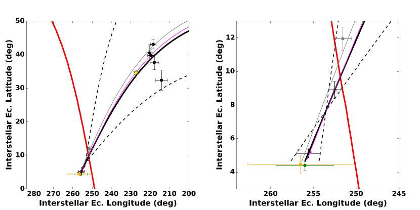
Figure 13: The interstellar magnetic field direction B_ism and the interstellar He^∘ velocity V_ism are offset from each other by 40^∘ and define the B_chm–V${}_{\mathrm{chm}}~{}$plane that characterizes the observed offsets between primary neutral interstellar populations and those that include secondary neutrals created by charge-exchange between magnetically deflected ions and interstellar neutrals. The thick red line shows the polarization band. The B_chm–V${}_{\mathrm{chm}}~{}$plane is shown for IBEX (thick black line and dashed lines) and Ulysses (pink line) He^∘ velocities, and for the ISMF direction (star) obtained from MHD models of the ribbon (Zirnstein et al., 2016). The energy-dependent centers of the IBEX ribbon (Funsten et al., 2013) are shown with the set of five cross symbols, with lowest/highest ENA energies correspond to the ribbon centers at the highest/lowest latitudes. The polarization band (thick red line) is approximately parallel to the elongated configuration of the IBEX energy-dependent ribbon centers. The warm secondary He^∘ breeze (gray dot) and mixed primary and secondary H^o population (from SOHO/SWAN data, open gray box) are offset along the B_chm–V${}_{\mathrm{chm}}~{}$plane, and away from the primary populations that anchor the B_chm–V${}_{\mathrm{chm}}~{}$plane at the lowest latitudes. The upwind directions of He^∘ from IBEX (black circle) and Ulysses(pink dot), and IBEX results for the interstellar O^o wind (orange and green dots) define the B_chm–V${}_{\mathrm{chm}}~{}$band at the lowest latitudes. The right figure is a zoomed version of the left figure. This figure is adapted from Schwadron et al. (2015b) and Schwadron & McComas (2017).

The 40^∘ angle between the heliocentric CHM velocity of interstellar neutrals (V_ism) and interstellar magnetic field direction (B_ism) leads to differences between the propagation of interstellar neutrals and charged particles through the outer heliosheath due to Lorentz forces. A warm breeze of secondary interstellar He^∘ atoms, originating mainly with interstellar helium ions displaced by Lorentz forces, was discovered by IBEX and confirmed by Ulysses (Kubiak et al., 2014; Schwadron et al., 2015a, 2016; Kubiak et al., 2016; Bzowski et al., 2017; Wood et al., 2017). The spatial offsets between the directions of primary and secondary neutrals are aligned with the B_chm–V${}_{\mathrm{chm}}~{}$plane (Figure 13, adapted from Schwadron et al., 2015b; Schwadron & McComas, 2017), The magnetic field direction in Figure 13 (star) is given by MHD models of the IBEX ribbon (Zirnstein et al., 2016). Primary He^∘ and O^o populations define the inflow direction of undeflected interstellar neutral. Secondary He^∘ neutrals (the warm breeze) are shifted along the B_chm–V${}_{\mathrm{chm}}~{}$plane due to the Lorentz deflection of parent ions (Kubiak et al., 2016; Bzowski et al., 2017; Wood et al., 2017). The H^o population is a mix of of primary and secondary atoms and is shifted along the B_chm–V${}_{\mathrm{chm}}~{}$plane (Lallement et al., 2010).

The great circle of the polarization band (red line) passes through the heliosphere nose (making an angle of $5.0^{\circ}\pm 6.7^{\circ}$ with respect to the upwind He^∘ directions). The polarization band also overlaps the direction of the warm breeze of secondary He^∘ atoms and the filament ISMF locations.

The polarization band is canted toward a different direction than the B-V plane but appears to have a similar slope as the locus of the energy-dependent centers of the IBEX ribbon (Funsten et al., 2013, five black crosses in Figure 13). The lowest energy ribbon data point (at 0.7 keV, see Schwadron et al., 2015b) deviates slightly from the alignment of the ribbon points (Figure 13).

The dipole component of the magnetic field of the filament of polarized dust grains (§4.2) is not plotted in Figure 13 but it coincides with the He^∘ warm breeze direction (the angle between the two directions is $5.2^{\circ}\pm 11.8^{\circ}$) so that the dust filament also traces the B-V plane. The B_chm–V${}_{\mathrm{chm}}~{}$plane appears to have an influence on the polarization band because they cross near the nose and warm breeze directions, but they trace different Lorentz forces because their slopes differ.

The deflection of interstellar dust grains by heliosheath magnetic fields is well established both observationally and theoretically, including a prediction of dust plumes around the heliosheath (Frisch et al., 1999; Landgraf, 2000a; Landgraf et al., 2000; Mann & Czechowski, 2004; Mann, 2010; Slavin et al., 2012; Krüger et al., 2015; Sterken et al., 2015; Alexashov et al., 2016).

6.4 Filament of Polarizing Dust

The filament polarizations (§4.2, Frisch et al., 2015b, a) and the warm breeze of deflected interstellar neutrals (Kubiak et al., 2014; Bzowski et al., 2015; Kubiak et al., 2016; Schwadron et al., 2016; Wood et al., 2017; Bzowski et al., 2017) trace the same interstellar upwind direction at the heliosphere nose (Table 1). The alignment of these two directions suggests that the parent interstellar ions of the secondary neutral atoms, and the charged interstellar dust grains, are trapped in the same interstellar magnetic field lines that are interacting with the heliosphere. Both populations would be guided through the outer heliosheath by mass-independent interactions with the draped interstellar magnetic field.

Warm breeze atoms survive to the inner heliosheath where they are measured by IBEX. Interstellar dust grains are also measured in the inner heliosphere so that it is possible some filament dust grains reach the inner heliosphere, where they would comprise the lower end of the interstellar dust mass spectrum detected in situ, and have been predicted by models of the entry and propagation of interstellar dust through the heliosphere (Frisch et al., 1999; Landgraf, 2000b; Mann & Czechowski, 2004; Slavin & Frisch, 2008; Slavin et al., 2012; Sterken et al., 2013; Ma et al., 2013; Krüger et al., 2015).

The filament polarizations possibly arise in the grains trapped in the laminar interstellar magnetic field observed in the outer heliosheath where Voyager 1 is approaching the interstellar medium (Burlaga et al., 2018), 30^∘ north of the heliosphere nose and in a sightline adjacent to the polarization band. Weak Kolmogorov turbulence observed by Voyager 1 is consistent with an outer scale corresponding to a cloud boundary at 0.01 pc. These low levels of magnetic turbulence in the outer heliosheath would minimize the disruption of grain alignment.

MHD models of dust propagation in the heliosphere predict deflected dust grains in these same locations (Slavin et al., 2012). Filament star polarizations are plotted in Figures 7 and 8. Five filament stars in the ecliptic-north of the heliosphere nose are also located toward the polarization band. Eight stars below the heliosphere nose (in ecliptic projection) have polarizations that veer northwards of the polarization band.

Interstellar magnetic field lines interacting with the heliosphere have different possible effects on dust grain polarizations. Twisted magnetic field lines and unorganized depolarization screens would have different effects on linearly polarized starlight. Thick foreground screens of randomly oriented dust grains will act to depolarize light. A twisted magnetic field in a thin low density region will also twist polarization position angles without disrupting the attachment of the grains to the magnetic field lines because of the long collisional timescales required for the grain to sweep up enough gas mass to disrupt the grain alignment. The low levels of magnetic turbulence found in the outer heliosheath by Voyager 1 (Burlaga et al., 2018) would minimize disruption of grain alignment.

Polarization strengths can arise from the photon path through interstellar clouds before reaching the heliosphere, but grains must stay tightly coupled to the ISMF interacting with the heliosphere to explain the polarization filament. The polarization strengths for nearby stars tend to be comparable to strengths expected from standard ratios between interstellar N(H^o), E(B-V), polarization strengths (footnote 1), however neither interstellar ions nor radiative torques are included in these standard relations (Frisch et al., 2015b).

6.5 Polarizations and the Voyager Low-frequency Plasma Emissions

During the years 1992–1994 the plasma wave instruments on the Voyager 1 and 2 spacecraft detected 12 sources of low-frequency radio emissions formed beyond the heliopause (see Kurth & Gurnett, 2003). Triangulation of source directions gave the locations of the emitting regions, which were found to be at 113–139 AU for the primary solutions, placing the events beyond the heliopause in the upwind regions of the heliosphere. The plasma oscillation frequency is consistent with electron plasma oscillations that originate from interstellar gas with density 0.08 cm^-3 (Gurnett et al., 2013, in agreement with models of the interstellar electron density at the heliosphere boundary, Slavin & Frisch 2008). The emissions arise from Langmuir waves initiated by the effects of the impact of plasma from a solar storm on the outer heliosheath region. A magnetic field direction that is not in the plane of the sky permits the propagation of Langmuir waves upstream of the heliopause (Mitchell et al., 2004). Kurth & Gurnett (2003) pointed out that the source regions of the low-frequency emissions were roughly aligned along the galactic plane. (The locations of the $\approx 3$kHz emissions are shown on the figures with asterisks). Most of these emission events (75%) are located close is to the equator of the polarization band, and on the port side of the heliosphere nose. The emissions on the starboard side of the heliosphere are located above the polarization band by ten degrees or more. The low frequency plasma emissions avoid tracing interstellar magnetic field directions near the plane of the sky for the $\Gamma$(L_rot,B_rot)$<0.63$ statistical criteria of Figures 7 and 8. The distance interval over which the radio emissions were detected (Kurth & Gurnett, 2003) is comparable to the distances predicted by 3D MHD heliosphere models of interstellar grains deflected around the heliosphere (Slavin et al., 2012). The geometric coincidence between the polarization band feature and most of the low frequency plasma emission events suggest they are affected by magnetic fields that are located in the same region of the outer heliosphere beyond the heliopause.

The heliosphere nose region clearly stands out as a region where values of $\theta_{\mathrm{rot}}$ are very small so that the interstellar magnetic field is quasi-parallel to the sightlines.

6.6 Impact of Loop I on Local Interstellar Magnetic Field

The encroachment of an expanding superbubble on the solar neighborhood, as indicated by both models and data describing Loop I (Frisch & Dwarkadas, 2018, FD18), should affect the ISMF within 15 pc. The interstellar magnetic field configuration in the tangential regions of the Loop I shell is well determined from polarized starlight that indicate the Loop I perimeter is a magnetically defined feature (Santos et al., 2011), which approaches to within 40 pc of the Sun near $\ell\sim 25^{\circ}$ if it is spherically symmetric (FD18]. The concentric circular lines in Figures 7 and 8 outline the X-ray feature in the sky that has been proposed as an interaction ring between Loop I and the Local Bubble (Egger & Aschenbach, 1995). The smallest angular sampling used here is $\pm 45^{\circ}$ (for $\Gamma$(L_rot,B_rot)$<0.10$, Figure 8) and shows that nearby regions interior to the innermost shell contour have preferred interstellar field orientations that are dominated by magnetic field angles larger than $\sim 37^{\circ}$ with respect to the sightlines (dark blue). The $\Gamma$(L_rot,B_rot)$<$$\Gamma_{\mathrm{max}}$=0.63 (Figure 6) indicates that the dominant blue regions inside of Loop I shell are within 40^∘ of the plane of the sky. The interior of Loop I and the location of highest heliosheath plasma pressures extend over similar regions of the sky.

Figure 6 shows maps of magnetic structure for $\Gamma$(L_rot,B_rot)$<0.63$ plotted with a logarithmic color scale. Those maps show that an elongated organized green polarization filament is found within 15 pc that corresponds to the eastern side of the southern part of Loop I, south of the galactic plane for figures in galactic coordinates. Equivalently this filament is east of the heliosphere nose for plots in ecliptic coordinates. The alignment of the local filament with the Loop I superbubble shell suggests strongly that Loop I has expanded to the solar location. Previous work has also shown that polarization strengths rise steadily with distance in this region (Bailey et al., 2010).

6.7 Magnetic Structure and Local Interstellar Medium

The role that magnetic fields play in the configuration of local interstellar clouds is not known. Striations or filaments that align with the direction of the interstellar magnetic field are common in high-latitude diffuse interstellar regions (Clark et al., 2016). Interstellar gas within 15 parsecs fills less than 20% of space, and is asymmetrically distributed around the heliosphere so that filamentary structures are allowed by the data. The closest interstellar cloud is the Local Interstellar Cloud (LIC, see footnote 2), which is observed mainly towards stars in the galactic anti-center hemisphere (Figures 7, 8). The LSR velocities of the gas and dust flowing through the heliosphere yield an upwind direction in the direction of the center of the Loop I superbubble (FRS11, Schwadron et al., 2014a). The angle between the heliocentric velocities of the CHM (Schwadron et al., 2015a)) and the LIC (Redfield & Linsky, 2008a) is $4.3^{\circ}\pm 2.6^{\circ}$. The absence of kinematical components at the LIC velocity toward the nearest star $\alpha$ Cen and toward 36 Oph, 7 pc beyond the heliosphere nose (Wood et al., 2000), has several possible explanations, including that the Sun is at the edge of the LIC for the nose direction of the heliosphere, that the CHM is not part of the LIC, or that rapid speed of the LIC through the LSR ($17.2\pm 1.9$ ${\rm km~{}s}^{-1}$) and the long collisional time scales (millions of years) decouple LIC neutrals from the LIC ions, which couple tightly to the magnetic field.

Note that the LIC border extends to the location of the IBEX interstellar magnetic field location, shown by the “B”, on maps with the highest spatial resolution of 45^∘ (Figure 8) and other maps. A transition to magnetic field orientations that are dominated primarily by angles within $\sim 37^{\circ}$ of the radial sightlines (low counts of data with $\Gamma$(L_rot,B_rot)$<$0.1) is found over most of the interior of the LIC above galactic latitudes of –60^∘. Figure 8 shows that the LIC does not extend to sightlines in front of the interior of the Loop I shell, which is dominated by high counts of data meeting the statistical condition $\Gamma$(L_rot,B_rot)$<0.10$ (green/blue regions). Results based on maps with $\Gamma$(L_rot,B_rot)$<0.63$ are consistent with those based on $\Gamma$(L_rot,B_rot)$<0.10$.

If the CHM belongs to the LIC then IBEX data show that the LIC and the interstellar magnetic field are perpendicular (§1). The interstellar magnetic field in the upwind direction of the LIC LSR motion should therefore be dominated by magnetic field directions that are quasi-parallel to the plane of the sky since the apex direction is 31^∘ from the ISMF defined by the IBEX ribbon. These results on the magnetic field orientation support such a configuration. IBEX data show that the interstellar magnetic field and LSR velocity vector of the CHM are perpendicular, with an upwind direction toward the center of the Loop I superbubble. LSR velocities of interstellar absorption lines in nearby stars indicate an upwind direction of the CLIC toward the Loop I superbubble (FRS11). The favored local ISMF direction toward the interior of the Loop I superbubble shell is quasi-parallel to the plane of the sky (Figures 6–8), which is consistent with the perpendicular relation between velocity and magnetic field direction directly observed by IBEX and favored for LIC and CLIC by the field directions displayed here.

6.8 Magnetic Field in BICEP2 Region

The spatial region searched by the BICEP2 experiment for evidence of B-mode polarizations of the cosmic microwave background signal (Ade & the BICEP2 team, 2014), is outlined with cyan-colored contours in Figures 7 and 8. The nearest 15 pc of the BICEP2 region contains a high percentage of polarization position angles with angles larger than 37^∘ with respect to the sightlines, according to the statistical criteria $\Gamma$(L_rot,B_rot)$<0.1$. Such a magnetic configuration would favor the detection of synchrotron emissions should they arise in this local region and would inhibit the detectability of Faraday rotations of background sources.

6.9 Small-Scale Structure in Cosmic Ray Data

IceCube IC59 maps of cosmic rays in the TeV–PeV energy range at declinations less than –30^∘ identified regions showing excesses of cosmic rays over small angular scales, 10^∘ or less (Abbassi & IceCube Collaboration, 2012; Aartsen & IceCube Collaboration, 2016). Figures 7, 8 show that the IC59 events arrived from directions that are outside of the LIC and where magnetic field directions with angles larger than $\sim$37^∘ with respect to sightlines dominate. The lack of IC59 sources inside of the LIC suggests that the LIC impedes the propagation of galactic cosmic rays to the heliosphere. It is not possible to make a clear-cut statement about the magnetic field orientation in the LIC using Figure 8, with an angular resolution of $\pm 45^{\circ}$, since a range of field directions are found inside of the cloud. Global properties of the magnetic field orientation outside of the LIC show extended regions where the magnetic field orientation is quasi-parallel to the plane of the sky. If the IceCube IC59 tiny structures originate in the interstellar medium then possible reconnection between magnetic fields may allow the inward-directing cosmic rays. The IC59 source angular widths of 10^∘ or smaller are not resolved by the maps in this paper.

The structure of the magnetic field surrounding the heliosphere impacts the propagation of PeV cosmic rays into the heliosphere. The interstellar magnetic field around the heliosphere will be frozen into the partially ionized CHM (n_e$\sim 0.08$ cm^-3, magnetic field strengths $\sim 3$ $\mu$G, FRS11). The 15-cloud model lacks interstellar absorption components at the LIC velocity towards nearby stars over most of the galactic center hemisphere. If the CHM is part of the LIC this indicates a distance to the LIC edge, 0.1 pc, that is comparable to the gyroradius of 2.5 PeV cosmic rays. The magnetic structure traced by the local polarization data will influence trajectories of cosmic rays with energies up to 250 PeV or more.

7 Summary and Conclusions

We have used new data from eight observatories in both hemispheres and data in the literature on linearly polarized starlight to map the structure of the local interstellar magnetic field within 15 pc. Magnetic structure is evaluated two ways, by evaluating sightlines where multiple stars predict the magnetic fields with the same orientation using statistical considerations, and with a least-squares-fit that finds the most probable magnetic field orientation for subsets of the data. Magnetic features have been discovered that can be attributed to the local interstellar medium and to the interaction between interstellar dust and the heliosphere. Magnetic structure maps are presented in three coordinate systems, galactic, ecliptic, and equatorial, to facilitate comparison with other sets of data.

The initial expectation for this study was that the interstellar polarizations of nearby star would reveal the structure of the ISMF in the interstellar medium within $\sim 15$ pc. This expectation proved to be incorrect and instead the most recognizable structures in these data are related to the heliosphere.

The primary results of this study are:

(1) A prominent polarization feature is found that consists of a polarization band (PB) that extends throughout much of the sky and displays magnetic field orientations that are quasi-perpendicular to the plane of the sky. The PB is more prominent in the first two Galactic quadrants and has a gap in the fourth galactic quadrant, corresponding to south of the ecliptic nose. The PB configuration can be described with a great circle that has an axis toward $\ell$=214^∘, $b$=67^∘, and is tilted by 23^∘ with respect to the galactic plane. A least squares fit to the best data tracing the polarization band yields the dipole component of the magnetic field aligned with $\lambda$= $247.0^{\circ},$ $\beta$=$82.2^{\circ}~{}(\pm 4.5^{\circ})$, which is close to the ecliptic poles. The PB also passes close to the heliosphere nose, to the dipole component of a magnetic field traced by a dusty filament, and to the direction of the warm breeze of secondary interstellar neutrals discovered by IBEX. Plots of the mean magnetic field direction along the polarization band show values within $\sim 30^{\circ}$ of the sightlines in the ecliptic north of the heliosphere nose.

(2) Seventy-five percent of the low-frequency kHz radio emissions discovered beyond the heliopause by the Voyager spacecraft follow the alignment of the polarization band. By coincidence the polarization band is close to the direction of Voyager I, and close to the direction of the solar apex motion.

(3) The geometrical relation between the polarization band and structure of the heliosphere strongly suggests that the polarization band represents a magnetic symmetry of the heliosphere that is traced by interstellar dust grains entrained in the ISMF interacting with and draping over the heliosphere. The PB separates the flow of dust between the port and starboard heliosphere flanks. Similar results for dust interacting with the heliosphere have been predicted by several theoretical studies.

(4) The nose region of the heliosphere stands out clearly as a region where the magnetic field direction, as traced by rotated polarization position angles, is quasi-parallel to sightlines. Mean polarization position angles in this region are within $\sim 30^{\circ}$ of sightlines

(5) Two regions selected from the IBEX ribbon configuration show magnetic field orientations that are inclined by more than $\sim 60^{\circ}$ with respect to sightlines.

(6) The magnetic structure of the LIC is not yet clear, but the boundaries of the LIC tend to correspond to regions where the ISMF is quasi-parallel to the plane of the sky, i.e. oriented more than 37^∘ from the sightlines. Maps with smaller sampling angles than the smallest values of $\pm 45^{\circ}$ in this paper are needed for more detailed comparisons between the LIC and magnetic structure.

(7) Filamentary magnetic structures that overlap the Loop I shell are found within 15 pc of the Sun. The interior of Loop I is dominated by magnetic field directions with angles larger than 37^∘ with respect to the sightlines. The Loop I interior also coincides with the region of highest heliosheath pressures identified by IBEX.

(8) Both the heliosphere nose region and a second region near $\ell$$\sim 280^{\circ}$, $b$$\sim 15^{\circ}$ stand out on the magnetic structure maps as regions that display predominantly interstellar magnetic field directions that are within about 19^∘ of the sightlines.

(9) The Ice Cube small scale cosmic ray sources (IC59) are located outside of the LIC and are found in locations where the dominant ISMF directions tend to have angles greater than 37^∘ with respect to the sightline. These cosmic ray sources also tend to be found in the region of highest heliosheath pressure. Maps with angular smoothing smaller than the smallest resolution, $\pm 45^{\circ}$, used in this study are needed to identify local magnetic field directions more precisely.

(10) The axis of the polarization band is directed toward the Leo cloud. A possibility for an interstellar origin of the polarization band is that the band geometry corresponds to the geometry of the kinematically defined Cetus Ripple found by Gry & Jenkins (2014a). However, the LSR velocity of the Cetus Ripple heliocentric velocity indicates that it flows away from the Aurigae cloud and is unrelated to the LIC.

(11) The polarization band does not appear to be related to the Cassini ENA belt, which has a tilt angle of about 30^∘ with respect to the galactic plane and does not follow a great circle.

The polarization band discovered here establishes that the interaction between the heliosphere and the interstellar medium creates an ordered magnetic structure that may cause a weak foreground contamination of astrophysical data that are sensitive to a magnetized and/or dusty plasma.

We have shown that our statistical filtering of the magnetic field directions traced by multiple polarization position angles is also capable of yielding quantitative information about the orientations of the local interstellar magnetic field. We have not yet mapped the extent of the ISMF that shapes the heliosphere. Sorting interstellar from the unexpected heliospheric contributions to the observed polarizations of nearby stars is required before the interstellar component of these weak polarizations are fully understood. Future studies will expand the general picture of ISMF orientations given in this paper and provide quantitative on the orientations of magnetic field directions on the sky as traced by polarization position angles.

Appendix A Statistical Probability Distribution

The merit function used to determine the probabilities that a polarization position angle measurement traces a magnetic field in a “true” direction is from Naghizadeh-Khouei & Clarke (1993):

$$G_{\mathrm{n}}(\theta_{\rm{obs}};~{}\theta_{\rm{o}},P_{\rm{o}})~{}=~{}\frac{1}{\sqrt{\pi}}~{}\{\frac{1}{\sqrt{\pi}}+\eta_{\rm{o}}~{}\rm{exp}(\eta^{2}_{\rm{o}})~{}[1+\rm{erf}(\eta_{\rm{o}})]\}\rm{exp}({-\frac{P^{2}_{\rm{o}}}{2}})$$ (A1)

The observed position angle is $\theta_{\rm{obs}}$, the “true” position angle is $\theta_{\rm{o}}$, and $P_{\mathrm{o}}=\frac{P_{\mathrm{true}}}{\sigma}$, mean error $\sigma$=dP, $\eta_{\mathrm{o}}~{}=~{}\frac{P_{\mathrm{o}}}{\sqrt{2}}~{}\mathrm{cos}~{}[2(\theta_{\mathrm{obs}}-\theta_{\mathrm{o}})]$, and the Gaussian error function $erf(Z)~{}=~{}\frac{2}{\sqrt{\pi}}\int_{0}^{Z}{exp}({-t^{2}})~{}dt$. Polarizations and position angles are derived from the Stokes parameters Q and U. The probability distribution function is non-Gaussian because of the bivariate nature of the position angle and the fact that polarizations are always positive while the underlying Stokes parameters can be positive or negative. The probability distribution function reverts to a Gaussian at large probabilities ($>6$).

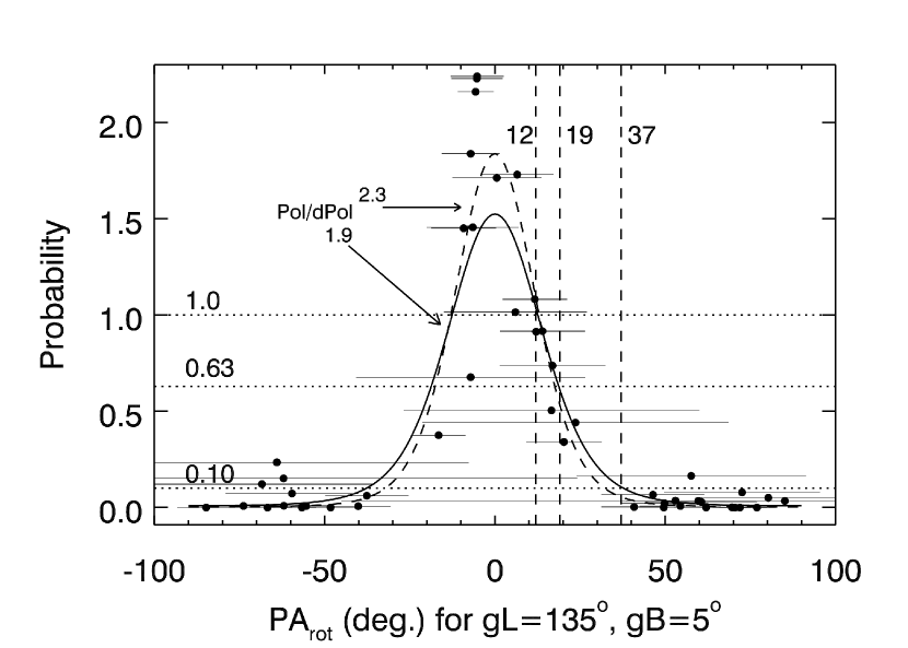
Figure 14: The probabilities $\Gamma$(L_rot,B_rot) that stars within 90^∘ of the location $L_{\mathrm{rot}}$=135^∘, $B_{\mathrm{rot}}$=5^∘ ($\lambda$,$\beta$=63^∘,46^∘, RA,DEC=42^∘,65^∘) trace an ISMF toward that location (ordinate) are plotted against polarization position angles rotated to that location, $\theta_{\mathrm{rot}}$ (abscissa). Values of $\theta_{\mathrm{rot}}$ for this set of stars are shown as dots. The solid (dashed) curves show the theoretical probability distributions for $P$/$dP$=1.9 (2.3) based on eqn. A1. Probability values 0.10, 0.63, and 1.0 are plotted with dotted horizontal lines as an illustration of the effect of $\Gamma_{\mathrm{min}}$ (or $\Gamma_{\mathrm{max}}$) on the selection of plotted data. The vertical dashed lines show the intersections of these probability values with the probability distributions. For example, stars with $\Gamma$(L_rot,B_rot)$>$$\Gamma_{\mathrm{min}}$=0.63 would tend to trace magnetic field directions that are within 19^∘ of the sightline, although the detailed cutoff angle depends on $P$/$dP$. Stars with $\Gamma$(L_rot,B_rot)$<$$\Gamma_{\mathrm{max}}$=0.1 will tend to trace magnetic field directions with angles that are larger than 37^∘ with respect to the sightlines, or alternatively within 53^∘ of the plane of the sky.

Theoretical probability distributions (eqn. A1) for $P$/$dP$=1.9 and $P$/$dP$=2.3 are shown in Figure 14, left, together with the rotated polarization position angles, $\theta_{\mathrm{rot}}$, for stars located within 60^∘ of the heliosphere nose (Table 1) corresponding to the statistical conditions used to construct Figure 7. The relative absence of data points with probabilities $\Gamma$(L_rot,B_rot)$>0.63$ for tracing an ISMF direction toward the nose of the heliosphere (Figure 14 may indicate the presence of a depolarizing screen covering the heliosphere nose region. Figure 14 also suggests that the statistical conditions $\Gamma$(L_rot,B_rot)$>$$\Gamma_{\mathrm{min}}$=1.0 and $\Gamma$(L_rot,B_rot)$>$1.5 used for Figure 4 to define directions near the magnetic field orientation (in green) yield values of $\theta_{\mathrm{rot}}$ that are within 10^∘–20^∘ of the sightlines. The detailed angle between the magnetic field orientation and the sightline depends on the $P$/$dP$ of individual stars and will be studied in more detail in a future study. The statistical conditions $\Gamma$(L_rot,B_rot)$<$$\Gamma_{\mathrm{max}}$=0.1 used in Figures 7–8 corresponds roughly to rotated polarization position angles $\theta_{\mathrm{rot}}$ at each grid point that have angles that are larger than 37^∘ with respect to the sightlines.

Examples of the probability distributions for $\theta_{\mathrm{rot}}$ are shown for sightlines toward the nose of the heliosphere and the LSR upwind direction for the CLIC in Figure 14. These distributions only include stars within 15 pc.

Appendix B Display of Supplementary Data

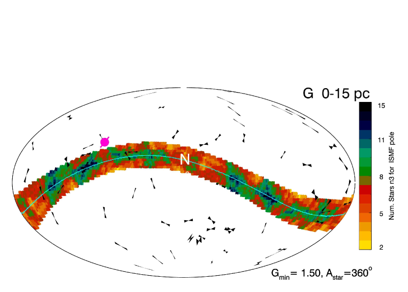
Figure 15: The subset of the overlapping polarization position angle swaths that fall within $\pm 10^{\circ}$ of the polarization band great circle (§3.1) are plotted. The polarization band was defined by the great circle that is 90^∘ from an axis located at $\ell$=214^∘, $b$=67^∘ (§3.1) and is created by enhanced numbers of overlapping polarization position angle swaths compared to adjacent regions. The triangular symbols show the locations and polarizations of all stars with polarization position angles that trace a magnetic field location within 10^∘ of the polarization band great circle. The highest quality subset of data that trace the polarization band are used for the least-square fits to the magnetic dipole component (§4.1). The pink dot shows the location of this best-fitting magnetic field direction, which is located close to the north ecliptic pole.

The polarization band was identified using the entire data set subject to the probability constraints, inclusive of the filament stars that trace interstellar dust grains interacting with the heliosphere (Frisch et al., 2015a). In an effort to understand the origin of the polarization band, the filament stars were omitted from the least-squares fitting process in §4.1. The great circle describing the polarization band was obtained from the entire data set used in this study, without omitting the filament stars. The dipole component of the magnetic pole obtained from the least-squares fit to the best stars tracing the polarization band (§4.1, Table 1) is $17.6^{\circ}\pm 6.6^{\circ}$ from the polarization band at the location of closest approach ($\ell$=83.4^∘, $b$=15.5^∘). The exclusion of the filament stars from the least-squares solution for the dipole component of the polarization band means that the polarization band and fitted dipole component are based on slightly different subsets of the data that will have slightly different geometries. There is no prior reason to predict that the axis of the polarization band defined by the polarization position angle swaths should correspond to the location of the dipolar magnetic field, especially since the overlapping position angle swaths that create the band do not intersect the polarization band at right angles (Figure 15). The position angle data that trace the polarization band are selected as those stars tracing an interstellar magnetic field falling within 10^∘ of the polarization band great circle. The polarization band is discovered in this study and has not been predicted, so that these results can not be compared to any formation model.

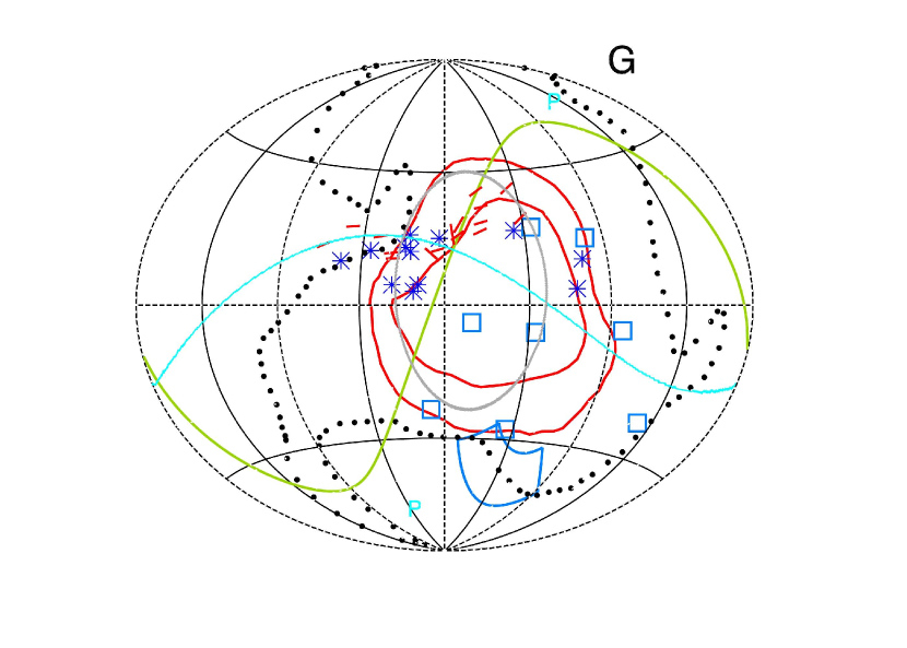
Figure 16: The supplementary data discussed in the main text are plotted in galactic coordinates and centered on the center of the galaxy. Phenomena displayed in this figure include the region of high heliosheath pressure found by IBEX (approximated with a gray circle, based on McComas & Schwadron, 2014), the LIC (dotted line), polarization band (cyan-colored curved line), ecliptic plane (curved green line), BICEP2 region (compact structure with blue curved lines), and outlines of the more distant regions of the Loop I shell (semi-concentric red lines, from Santos et al., 2011). Blue squares show locations of IC59 small scale cosmic ray sources. The blue asterisks show locations of the Voyager 1, 2 low frequency emission events. The red bars show the polarizations of a filament of interstellar dust grains draped over the heliosphere. See the text for more information.

These auxiliary data that trace structure in the heliosphere are discussed in the text and plotted on many figures. Here we show the auxiliary data alone, without data on magnetic structure. Figure 16 shows the auxiliary data plotted in galactic coordinates, and centered on the center of the galaxy. Shown on this figure are the LIC (irregular dotted line, Redfield & Linsky, 2008b), the two semi-concentric outlines of Loop I identified by Egger & Aschenbach (1995) and carefully mapped in polarization data by Santos et al. (2011, semi-circular red concentric lines), the outline of the low opacity BICEP2 region that has served as a probe of the cosmic microwave background emission (blue closed curved lines, Ade & the BICEP2 team, 2014), and the IceCube IC59 measurements of small scale structure in the TeV cosmic ray data (blue squares, Abbassi & IceCube Collaboration, 2012; Aartsen & IceCube Collaboration, 2016). The low frequency kHz emissions detected by Voyager 1 and Voyager 2 are plotted as blue asterisks. The three-dimensional positions of these emissions were found to most likely be located upstream of the heliopause, according to triangulation arguments applied to the measurements made with the two spacecraft in different locations (Gurnett et al., 1993; Kurth & Gurnett, 2003). The red bars show polarization data that have been identified as arising from a dusty magnetic filament that is interacting with the heliosphere (Frisch et al., 2015b, a). Some of the stars tracing this magnetic filament are located beyond the 15 pc scope of this paper. The curved cyan-colored line shows the polarization band and the green curved line shows the location of the ecliptic plane on this galactic projection.

Appendix C Configuration of Cassini ENA Belt vs. Polarization Band

Cassini mapped global ENAs in the energy range 5.2–55 keV and found a “belt” configuration that is parallel to the galactic plane (Dialynas et al., 2017). The belt forms beyond the heliopause and consists of ENAs created by charge-exchange between interstellar neutral hydrogen atoms and the inner heliosheath 28–53 keV ion population measured by Voyager 1 and Voyager 2. Krimigis et al. (2009) and Dialynas et al. (2013) discuss the belt as a great circle, tilted by about 30^∘ with respect to the galactic plane and centered near ecliptic coordinates of $\lambda$=190^∘, $\beta$=15^∘ ($\ell$=310^∘, 72^∘ in galactic coordinates). The Cassini ENA belt is thick and irregular, and disappears at the lowest ecliptic latitudes (Dialynas et al., 2017) where the mean polarization position angles tends to be parallel to sightlines (Figure 12. The Cassini belt also roughly follows a circle of 77^∘ radius, with an axis at $\ell$,$b$=$110^{\circ},-67^{\circ}$ (ecliptic coordinates $\lambda$= 185^∘, $\beta$=–7^∘). The axes of these two different descriptions of the Cassini belt are consistent to within 10^∘. It is clear that the polarization band and the Cassini belt do not share the same geometry because of their different tilts compared to the galactic plane (23^∘ and 30^∘ respectively).

Surprisingly, the axis of the Cassini belt is within 6.2^∘ of the heliocentric velocity of the Cetus Ripple disturbance identified by (Gry & Jenkins, 2014a). Heliocentric velocities are suitable for describing physical interactions that take place in the inertial frame of the solar system. The fact that the Cassini belt has an axis near the Cetus Ripple heliocentric velocity vector allows the possibility that the shock proposed by Gry and Jenkins to explain the Cetus Ripple could also be influencing the heliosphere.

Appendix D Distribution of Stars within 15 pc

The results reported here on the orientations of the interstellar magnetic field are not the result of the distribution of the stars from which these conclusions are drawn. Figure 17 shows the number of stars that are within 60^∘ of each location $L_{\mathrm{rot}}$, $B_{\mathrm{rot}}$ and that have $P$/$dP$$>1.9$. The figure is in equatorial coordinates. The north/south pattern of the distribution of stars is partly a reflection of the different times of the year for good observing conditions in the northern versus southern hemisphere, and is unrelated to the magnetic structure traced by these linear polarization data.

Table 1: Summary of Interstellar Directions

Observable	Direction	Direction	Direction	Ref.
	$\ell$,$b$ (deg)	$\lambda,\beta$ (deg)	RA,DEC (deg)
Axis of polarization band	214, 67	158, 17	167, 24	1
Polarization band dipole component	$87.9,32.6(\pm 4.5)$	247.0, 82.2 $(\pm 4.5)$	264.0, 59.2 ($\pm 4.5)$	1
Filament direction	$5.9\pm 8.2$, $17.0\pm 3.5$	$255.0\pm 7.0$, $7.9\pm 8.5$	348.4, 17.9 $(\pm 8.9)$	1
IBEX Ribbon ISMF	$26.0\pm 0.7$, $50.1\pm 0.6$	227.3, 34.6 ($\pm 0.9$)	234.4, 16.3	2
IBEX interstellar He∘nose	$3.7\pm 0.9$, $15.1\pm 1.3$	$254.9\pm 1.5$, $5.12\pm 0.27$	$254.9\pm 1.5$, $-17.6\pm 0.4$	3
IBEX Warm He∘ breeze	8.0, 21.8 $(\pm 7.8)$	251, 12.0 $(\pm 7.8)$	251.7,–10.3 $(\pm 7.8)$	4
Heliosphere Maximum Pressure	347, 6	255, –14	252, –36	5
Upwind CHM HC direction	$3.7\pm 0.9$, $15.1\pm 1.3$	$255.6\pm 1.4$, $5.1\pm 0.27$	$254.9\pm 1.5$, $17.6\pm 0.4$	6
Upwind CLIC LSR direction	$335.6\pm 13.4$, $-7.0\pm 9.0$	260.3, -30.1 ($\pm 16.1$)	255.9, –53.0 ($\pm 16.1$	7

.

Figure 17: The distributions of stars used in this study are shown in equatorial coordinates, with zero degrees RA at the figure right. The figure shows counts of the number of stars within 60^∘ of each grid point $L_{\mathrm{rot}}$, $B_{\mathrm{rot}}$ for stars with $P$/$dP$$>$1.9. The target star grouping shows that the magnetic structure identified in this paper is unrelated to the spatial distribution of the target stars.

References

- Aartsen & IceCube Collaboration (2016) Aartsen, R. & IceCube Collaboration. 2016, ApJ, 826, 220
- Abbassi & IceCube Collaboration (2012) Abbassi, R. & IceCube Collaboration. 2012, ApJ, 746, 33
- Ade & the BICEP2 team (2014) Ade, P. A. R. & the BICEP2 team. 2014, Physical Review Letters, 112, 241101
- Alexashov et al. (2016) Alexashov, D. B., Katushkina, O. A., Izmodenov, V. V., & Akaev, P. S. 2016, MNRAS, 458, 2553
- Altobelli et al. (2016) Altobelli, N., Postberg, F., & et al. 2016, Science, 352, 312
- Andersson et al. (2015) Andersson, B.-G., Lazarian, A., & Vaillancourt, J. E. 2015, ARA&A, 53, 501
- Bailey et al. (2017) Bailey, J., Cotton, D. V., & Kedziora-Chudczer, L. 2017, MNRAS, 465, 1601
- Bailey et al. (2015) Bailey, J., Kedziora-Chudczer, L., Cotton, D. V., Bott, K., Hough, J. H., & Lucas, P. W. 2015, MNRAS, 449, 3064
- Bailey et al. (2010) Bailey, J., Lucas, P. W., & Hough, J. H. 2010, MNRAS, 405, 2570
- Berdyugin et al. (2014) Berdyugin, A., Piirola, V., & Teerikorpi, P. 2014, A&A, 561, A24
- Bohlin et al. (1978) Bohlin, R. C., Savage, B. D., & Drake, J. F. 1978, ApJ, 224, 132
- Burlaga et al. (2018) Burlaga, L. F., Florinski, V., & Ness, N. F. 2018, ApJ, 854, 20
- Burlaga & Ness (2014) Burlaga, L. F. & Ness, N. F. 2014, ApJ, 784, 146
- Burlaga & Ness (2016) —. 2016, ApJ, 829, 136
- Bzowski et al. (2017) Bzowski, M., Kubiak, M. A., Czechowski, A., & Grygorczuk, J. 2017, ApJ, 845, 15
- Bzowski et al. (2015) Bzowski, M., Swaczyna, P., Kubiak, M. A., Sokół, J. M., Fuselier, S. A., Galli, A., Heirtzler, D., Kucharek, H., Leonard, T. W., McComas, D. J., Möbius, E., Schwadron, N. A., & Wurz, P. 2015, ApJS, 220, 28
- Clark et al. (2016) Clark, S. E., Peek, J. E. G., Hill, J. C., & Putman, M. E. 2016, in IAU Symposium, Vol. 315, From Interstellar Clouds to Star-Forming Galaxies: Universal Processes?, ed. P. Jablonka, P. André, & F. van der Tak, E13
- Cohen (1995) Cohen, M. 1995, ApJ, 444, 874
- Cotton et al. (2017a) Cotton, D. V., Bailey, J., Howarth, I.-D., Bott, K., Kedziora-Chudczer, L., Lucas, P. W., & Hough, J. H. 2017a, Nature Astronomy, 1, 690
- Cotton et al. (2016) Cotton, D. V., Bailey, J., Kedziora-Chudczer, L., Bott, K., Lucas, P. W., Hough, J. H., & Marshall, J. P. 2016, MNRAS, 455, 1607
- Cotton et al. (2017b) Cotton, D. V., Marshall, J. P., Bailey, J., Kedziora-Chudczer, L., Bott, K., Marsden, S. C., & Carter, B. D. 2017b, MNRAS, 467, 873
- Dialynas et al. (2017) Dialynas, K., Krimigis, S. M., Mitchell, D. G., Decker, R. B., & Roelof, E. C. 2017, Nature Astronomy, 1, 0115
- Dialynas et al. (2013) Dialynas, K., Krimigis, S. M., Mitchell, D. G., Roelof, E. C., & Decker, R. B. 2013, ApJ, 778, 40
- Egger & Aschenbach (1995) Egger, R. J. & Aschenbach, B. 1995, A&A, 294, L25
- Fosalba et al. (2002) Fosalba, P., Lazarian, A., Prunet, S., & Tauber, J. A. 2002, ApJ, 564, 762
- Frisch & Dwarkadas (2018) Frisch, P. & Dwarkadas, V. V. 2018, ArXiv e-prints
- Frisch et al. (2005) Frisch, P., Grün, E., & Hoppe, P. 2005, Interstellar and Presolar Grains in the Galaxy and in the Solar System (The Solar System and Beyond: Ten Years of ISSI: Eds. J. Geiss and B. Hultqvist, ESTEC), 193–196
- Frisch et al. (2012) Frisch, P. C., Andersson, B.-G., Berdyugin, A., Piirola, V., DeMajistre, R., Funsten, H. O., Magalhaes, A. M., Seriacopi, D. B., McComas, D. J., Schwadron, N. A., Slavin, J. D., & Wiktorowicz, S. J. 2012, ApJ, 760, 106
- Frisch et al. (2015a) Frisch, P. C., Andersson, B.-G., Berdyugin, A., Piirola, V., Funsten, H. O., Magalhaes, A. M., Seriacopi, D. B., McComas, D. J., Schwadron, N. A., Slavin, J. D., & Wiktorowicz, S. J. 2015a, ApJ, 805, 60(8pp)
- Frisch et al. (2015b) Frisch, P. C., Berdyugin, A., Piirola, V., Magalhaes, A. M., Seriacopi, D. B., Wiktorowicz, S. J., Andersson, B., Funsten, H. O., McComas, D. J., Schwadron, N. A., Slavin, J. D., Hanson, A. J., & Fu, C.-W. 2015b, ApJ, 814, 112
- Frisch et al. (2016) Frisch, P. C., Berdyugin, A. B., Piirola, V., Magalhaes, A. M., Seriacopi, D. B., Ferrari, T., Santos, F. P., Schwadron, N. A., Funsten, H. O., McComas, D. J., & Heiles, C. E. 2016, in Journal of Physics Conference Series, Vol. 767, Journal of Physics Conference Series, 012010
- Frisch et al. (1999) Frisch, P. C., Dorschner, J. M., Geiss, J., Greenberg, J. M., Grün, E., Landgraf, M., Hoppe, P., Jones, A. P., Krätschmer, W., Linde, T. J., Morfill, G. E., Reach, W., Slavin, J. D., Svestka, J., Witt, A. N., & Zank, G. P. 1999, ApJ, 525, 492
- Frisch et al. (2011) Frisch, P. C., Redfield, S., & Slavin, J. 2011, ARA&A, 49
- Frisch & Schwadron (2014) Frisch, P. C. & Schwadron, N. A. 2014, in Astronomical Society of the Pacific Conference Series, Vol. 484, Outstanding Problems in Heliophysics: From Coronal Heating to the Edge of the Heliosphere, ed. Q. Hu & G. P. Zank, 42
- Frisch & Slavin (2006) Frisch, P. C. & Slavin, J. D. 2006, Short Term Variations in the Galactic Environment of the Sun, in Solar Journey: The Significance of Our Galactic Environment for the Heliosphere and Earth, ed. P. C. Frisch (Springer), 133–193
- Funsten et al. (2009) Funsten, H. O., Allegrini, F., Crew, G. B., DeMajistre, R., Frisch, P. C., Fuselier, S. A., Gruntman, M., Janzen, P., McComas, D. J., Möbius, E., Randol, B., Reisenfeld, D. B., Roelof, E. C., & Schwadron, N. A. 2009, Science, 326, 964
- Funsten et al. (2013) Funsten, H. O., DeMajistre, R., Frisch, P. C., Heerikhuijsen, J., Higdon, D. M., Janzen, P., Larsen, B., Livadiotis, G., McComas, D. J., Möbius, E., Reese, C., Reisenfeld, D. B., Schwadron, N. A., & Zirnstein, E. J. 2013, ApJ, 776, 30
- Fuselier et al. (2009) Fuselier, S. A., Allegrini, F., Funsten, H. O., Ghielmetti, A. G., Heirtzler, D., Kucharek, H., Lennartsson, O. W., McComas, D. J., Möbius, E., Moore, T. E., Petrinec, S. M., Saul, L. A., Scheer, J. A., Schwadron, N., & Wurz, P. 2009, Science, 326, 962
- Gayley et al. (1997) Gayley, K. G., Zank, G. P., Pauls, H. L., Frisch, P. C., & Welty, D. E. 1997, ApJ, 487, 259
- Gry & Jenkins (2014a) Gry, C. & Jenkins, E. B. 2014a, ArXiv e-prints
- Gry & Jenkins (2014b) —. 2014b, A&A, 567, A58
- Gry & Jenkins (2017) —. 2017, A&A, 598, A31
- Gurnett et al. (1993) Gurnett, D. A., Kurth, W. S., Allendorf, S. C., & Poynter, R. L. 1993, Science, 262, 199
- Gurnett et al. (2013) Gurnett, D. A., Kurth, W. S., Burlaga, L. F., & Ness, N. F. 2013, Science, 341, 1489
- Heger (1919) Heger, M. L. 1919, PASP, 31, 304
- Heiles (1996) Heiles, C. 1996, ApJ, 462, 316
- Heiles (2000) —. 2000, AJ, 119, 923
- Hoang & Lazarian (2016) Hoang, T. & Lazarian, A. 2016, ApJ, 831, 159
- Kimura et al. (2003) Kimura, H., Mann, I., & Jessberger, E. K. 2003, ApJ, 582, 846
- Krimigis et al. (2009) Krimigis, S. M., Mitchell, D. G., Roelof, E. C., Hsieh, K. C., & McComas, D. J. 2009, Science, 326, 971
- Krüger et al. (2015) Krüger, H., Strub, P., Gruen, E., & Sterken, V. J. 2015, ApJ, 812
- Kubiak et al. (2014) Kubiak, M. A., Bzowski, M., Sokół, J. M., Swaczyna, P., Grzedzielski, S., Alexashov, D. B., Izmodenov, V. V., Moebius, E., Leonard, T., Fuselier, S. A., Wurz, P., & McComas, D. J. 2014, ArXiv e-prints
- Kubiak et al. (2016) Kubiak, M. A., Swaczyna, P., Bzowski, M., Sokół, J. M., Fuselier, S. A., Galli, A., Heirtzler, D., Kucharek, H., Leonard, T. W., McComas, D. J., Möbius, E., Park, J., Schwadron, N. A., & Wurz, P. 2016, ApJS, 223, 25
- Kurth & Gurnett (2003) Kurth, W. S. & Gurnett, D. A. 2003, J. Geophys. Res., 108, 2
- Lallement et al. (1995) Lallement, R., Ferlet, R., Lagrange, A. M., Lemoine, M., & Vidal-Madjar, A. 1995, A&A, 304, 461
- Lallement et al. (2010) Lallement, R., Quémerais, E., Koutroumpa, D., Bertaux, J., Ferron, S., Schmidt, W., & Lamy, P. 2010, Twelfth International Solar Wind Conference, 1216, 555
- Landgraf (2000a) Landgraf, M. 2000a, J. Geophys. Res., 105, 10303
- Landgraf (2000b) —. 2000b, J. Geophys. Res., 105, 10303
- Landgraf et al. (1999) Landgraf, M., Augustsson, K., Grün, E., & Gustafson, B. Å. S. 1999, Science, 286, 2319
- Landgraf et al. (2000) Landgraf, M., Baggaley, W. J., Grün, E., Krüger, H., & Linkert, G. 2000, J. Geophys. Res., 105, 10343
- Lazarian (2007) Lazarian, A. 2007, J. Quant. Spec. Radiat. Transf., 106, 225
- Leroy (1993) Leroy, J. L. 1993, A&AS, 101, 551
- Ma et al. (2013) Ma, Q., Matthews, L. S., Land, V., & Hyde, T. W. 2013, ApJ, 763, 77
- Magalhaes et al. (1996) Magalhaes, A. M., Rodrigues, C. V., Margoniner, V. E., Pereyra, A., & Heathcote, S. 1996, in Astronomical Society of the Pacific Conference Series, Vol. 97, Polarimetry of the Interstellar Medium, ed. W. G. Roberge & D. C. B. Whittet, 118–+
- Mann (2010) Mann, I. 2010, ARA&A, 48, 173
- Mann & Czechowski (2004) Mann, I. & Czechowski, A. 2004, in AIP Conf. Proc. 719: Physics of the Outer Heliosphere, 53–58
- Marshall et al. (2016) Marshall, J. P., Cotton, D. V., Bott, K., Ertel, S., Kennedy, G. M., Wyatt, M. C., del Burgo, C., Absil, O., Bailey, J., & Kedziora-Chudczer, L. 2016, ApJ, 825, 124
- Mathewson & Ford (1970) Mathewson, D. S. & Ford, V. L. 1970, MmRAS, 74, 139
- McComas et al. (2009) McComas, D. J., Allegrini, F., Bochsler, P., Bzowski, M., Christian, E. R., Crew, G. B., DeMajistre, R., Fahr, H., Fichtner, H., Frisch, P. C., Funsten, H. O., Fuselier, S. A., Gloeckler, G., Gruntman, M., Heerikhuisen, J., Izmodenov, V., Janzen, P., Knappenberger, P., Krimigis, S., Kucharek, H., Lee, M., Livadiotis, G., Livi, S., MacDowall, R. J., Mitchell, D., Möbius, E., Moore, T., Pogorelov, N. V., Reisenfeld, D., Roelof, E., Saul, L., Schwadron, N. A., Valek, P. W., Vanderspek, R., Wurz, P., & Zank, G. P. 2009, Science, 326, 959
- McComas & Schwadron (2014) McComas, D. J. & Schwadron, N. A. 2014, ApJ, 795, L17
- McComas et al. (2017) McComas, D. J., Zirnstein, E. J., Bzowski, M., Dayeh, M. A., Funsten, H. O., Fuselier, S. A., Janzen, P. H., Kubiak, M. A., Kucharek, H., Möbius, E., Reisenfeld, D. B., Schwadron, N. A., Sokół, J. M., Szalay, J. R., & Tokumaru, M. 2017, ApJS, 229, 41
- Mitchell et al. (2004) Mitchell, J. J., Cairns, I. H., & Robinson, P. A. 2004, Journal of Geophysical Research (Space Physics), 109, 6108
- Naghizadeh-Khouei & Clarke (1993) Naghizadeh-Khouei, J. & Clarke, D. 1993, A&A, 274, 968
- Pereyra & Magalhães (2007) Pereyra, A. & Magalhães, A. M. 2007, ApJ, 662, 1014
- Perryman (1997) Perryman, M. A. C. 1997, A&A, 323, L49
- Piirola (1973) Piirola, V. 1973, A&A, 27, 383
- Piirola (1977) —. 1977, A&AS, 30, 213
- Piirola et al. (2014) Piirola, V., Berdyugin, A., & Berdyugina, S. 2014, in Society of Photo-Optical Instrumentation Engineers (SPIE) Conference Series, Vol. 9147, Society of Photo-Optical Instrumentation Engineers (SPIE) Conference Series, 8
- Plaszczynski et al. (2014) Plaszczynski, S., Montier, L., Levrier, F., & Tristram, M. 2014, MNRAS, 462, 4048=4056
- Pogorelov et al. (2011) Pogorelov, N. V., Heerikhuisen, J., Zank, G. P., Borovikov, S. N., Frisch, P. C., & McComas, D. J. 2011, ApJ, 742, 104
- Redfield & Linsky (2008a) Redfield, S. & Linsky, J. L. 2008a, ApJ, 673, 283
- Redfield & Linsky (2008b) —. 2008b, ApJ, 673, 283
- Santos et al. (2011) Santos, F. P., Corradi, W., & Reis, W. 2011, ApJ, 728, 104
- Schwadron et al. (2014a) Schwadron, N. A., Adams, F. C., Christian, E. R., Desiati, P., Frisch, P., Funsten, H. O., Jokipii, J. R., McComas, D. J., Moebius, E., & Zank, G. P. 2014a, Science, 343, 988
- Schwadron et al. (2009) Schwadron, N. A., Bzowski, M., Crew, G. B., Gruntman, M., Fahr, H., Fichtner, H., Frisch, P. C., Funsten, H. O., Fuselier, S., Heerikhuisen, J., Izmodenov, V., Kucharek, H., Lee, M., Livadiotis, G., McComas, D. J., Moebius, E., Moore, T., Mukherjee, J., Pogorelov, N. V., Prested, C., Reisenfeld, D., Roelof, E., & Zank, G. P. 2009, Science, 326, 966
- Schwadron & McComas (2017) Schwadron, N. A. & McComas, D. J. 2017, ApJ, 135, 135
- Schwadron et al. (2016) Schwadron, N. A., Möbius, E., McComas, D. J., Bochsler, P., Bzowski, M., Fuselier, S. A., Livadiotis, G., Frisch, P., Müller, H.-R., Heirtzler, D., Kucharek, H., & Lee, M. A. 2016, ApJ, 828, 81
- Schwadron et al. (2014b) Schwadron, N. A., Moebius, E., & Fuselier, S. A. e. a. 2014b, ApJ, in press
- Schwadron et al. (2015a) Schwadron, N. A., Moebius, E., Leonard, T., Fuselier, S. A., McComas, D. J., Heirtzler, D., Kucharek, H., Rahmanifard, F., Bzowski, M., Kubiak, M. A., Sokol, J., Swaczyna, P., & Frisch, P. 2015a, ApJS, 220, 25
- Schwadron et al. (2015b) Schwadron, N. A., Richardson, J. D., Burlaga, L. F., McComas, D. J., & Moebius, E. 2015b, ApJ, 813, L20
- Serkowski et al. (1975) Serkowski, K., Mathewson, D. S., & Ford, V. L. 1975, ApJ, 196, 261
- Slavin & Frisch (2008) Slavin, J. D. & Frisch, P. C. 2008, A&A, 491, 53
- Slavin et al. (2012) Slavin, J. D., Frisch, P. C., Müller, H.-R., Heerikhuisen, J., Pogorelov, N. V., Reach, W. T., & Zank, G. 2012, ApJ, 760, 46
- Sterken et al. (2013) Sterken, V. J., Altobelli, N., Kempf, S., Krüger, H., Srama, R., Strub, P., & Grün, E. 2013, A&A, 552, A130
- Sterken et al. (2015) Sterken, V. J., Strub, P., Krüger, H., von Steiger, R., & Frisch, P. 2015, ApJ, 812
- Stone & Cummings (2013) Stone, E. C. & Cummings, A. C. e. a. 2013, Science, 341, 150
- Tinbergen (1982) Tinbergen, J. 1982, A&A, 105, 53
- Wiktorowicz & Matthews (2008) Wiktorowicz, S. J. & Matthews, K. 2008, PASP, 120, 1282
- Wiktorowicz & Nofi (2015) Wiktorowicz, S. J. & Nofi, L. A. 2015, ApJ, 800, L1
- Wood et al. (2000) Wood, B. E., Linsky, J. L., & Zank, G. P. 2000, ApJ, 537, 304
- Wood et al. (2017) Wood, B. E., Müller, H.-R., & Witte, M. 2017, ApJ, 851, 35
- Wood et al. (2005) Wood, B. E., Redfield, S., Linsky, J. L., Müller, H.-R., & Zank, G. P. 2005, ApJS, 159, 118
- Yu (1974) Yu, G. 1974, ApJ, 194, 187
- Zirnstein et al. (2016) Zirnstein, E. J., Heerikhuisen, J., Funsten, H. O., Livadiotis, G., McComas, D. J., & Pogorelov, N. V. 2016, ApJ, 818, L18