Deformed Fokker-Planck equation: inhomogeneous medium with a position-dependent mass

Abstract

We present the Fokker-Planck equation (FPE) for an inhomogeneous medium with a position-dependent mass particle by making use of the Langevin equation, in the context of a generalized deformed derivative for an arbitrary deformation space where the linear (nonlinear) character of the FPE is associated with the employed deformed linear (nonlinear) derivative. The FPE for an inhomogeneous medium with a position-dependent diffusion coefficient is equivalent to a deformed FPE within a deformed space, described by generalized derivatives, and constant diffusion coefficient. The deformed FPE is consistent with the diffusion equation for inhomogeneous media when the temperature and the mobility have the same position-dependent functional form as well as with the nonlinear Langevin approach. The deformed version of the $H$-theorem permits to express the Boltzmann-Gibbs entropic functional as a sum of two contributions, one from the particles and the other from the inhomogeneous medium. The formalism is illustrated with the infinite square well and the confining potential with linear drift coefficient. Connections between superstatistics and position-dependent Langevin equations are also discussed.

I Introduction

Diffusion is understood as the thermal motion of particles, which is macroscopically translated into a net flux from one region to another. The standard way to quantify this phenomenon is to consider that the particles are subjected to drag (properly of the fluid) and random (Brownian motion) forces, which gives place to the Langevin equation Langevin-1908 . To link this classical description with a probabilistic characterization, the usual strategy is to rewrite the Langevin equation in terms of the probability density function (PDF), thus obtaining the Fokker-Planck equation (FPE) Risken . The FPE has been widely investigated in the literature, mainly applied to the study of different types of diffusion, including the normal and anomalous ones (associated to linear and nonlinear FPE) Scher-Montroll-1975 ; Plastino-Plastino-1995 ; Tsallis-Bukmann-1996 ; Borland-PRE-1998 ; Borland-PLA-1998 ; DeVoe-2009 . Subsequent applications in multiple kinds of phenomena have displayed the relevance of the FPE in the field of statistical physics Frank-2005 ; Muskat ; Klemm-Muller-Kimmich-1997 ; Barrozo-Moreira-Aguiar-AndradeJr-2009 ; Tsallis-1988 ; Tsallis-2009 ; Andrade-Silva-Moreira-Nobre-Curado-2010 . In particular, the FPE in a specific medium have presented an increasing interest since it allows to characterize electron diffusion Hizanidis-1989 , photoinduction in nonequilibrium processes Jang-2016 , rarefied gases and heterogeneous media Suciu-Radu-Attinger-Schuler-Knabner-2015 ; Collyer-Connaughton-Lockerbyco-2016 , interfaces-membranes Grassi-Raudino-2014 , multiple diffusion from fractional kernel operators Maike-2018 , superfast diffusion in porous media Xu-2019 , among others.

In addition, theoretical investigations have shown an intimate connection between generalized FPE, $H$-theorem, master equations and entropic forms, highlighting the role played by the nonextensive statistics Frank-2001 ; Schwammle-Curado-Nobre-2007 ; Ribeiro-Nobre-Curado-2011 ; Sicuro-Rapcan-Tsallis-2016 . Along to this progresses, the mathematical structure inherited by nonextensive statistics turned out to be a useful tool to generalize concepts of statistical mechanics. Some mathematical structures have been presented Nivanen-Mehaute-Wang-2003 ; Borges-2004 ; Tsallis-1994 ; Lobao-Cardoso-Pinho-Borges-2009 ; Tempesta-2011 , referred to as generalized algebras.

Parallel to this developments, the research on systems with a position-dependent effective mass emerged for describing transport phenomena in semiconductors heterostructures Bastard-1975 ; vonRoos-1983 provided with a position-dependent chemical composition. The starting point of this approach was the Wannier-Slater theorem for the wave function of the conduction band in homogeneous semiconductors, from which its extension to an inhomogeneous one led to several ways for defining the kinetic energy operator vonRoos-1983 . This ambiguity, called the ordering problem, was unified together with the requirement of hermiticity by von Roos vonRoos-1983 . Recently, from a particular case of the von Roos kinetic energy operator, a deformed Schrödinger equation for position-dependent mass has been studied CostaFilho-Almeida-Farias-AndradeJr-2011 ; CostaFilho-Alencar-Skagerstam-AndradeJr-2013 ; Barbagiovanni-2014 ; Costa-Borges-2014 ; Costa-Borges-2018 ; Costa-Gomez-2018 ; Nascimento-Ferreira-Aguiar-Guedes-CostaFilho-2018 ; Costa-Gomez-Santos-2020 and linked with a generalized translation operator inherited by the generalized $q$-algebra Nivanen-Mehaute-Wang-2003 ; Borges-2004 ; Tsallis-1994 ; Lobao-Cardoso-Pinho-Borges-2009 ; Tempesta-2011 . Position-dependent mass systems have been proven to be a useful theoretical tool in multiple areas and fairly fitting to experimental data: density functional theory Bencheikh-2004 , supersymmetric quantum mechanics Ioffe-2016 , nuclear physics Alimohammadi-2017 , nonlinear optics Li-2017 , Landau quantization Mustafa-2020 , among others.

The goal of this paper is to present the FPE for an inhomogeneous medium with a variable diffusion coefficient within the position-dependent mass scenario CostaFilho-Almeida-Farias-AndradeJr-2011 ; CostaFilho-Alencar-Skagerstam-AndradeJr-2013 ; Costa-Borges-2014 ; Costa-Borges-2018 ; Costa-Gomez-2018 , by means of a generalized deformed derivative, where the deformation of the space univocally determines the mass as well as the dumping and the diffusion coefficients. As a consequence, we find an equivalence between the FPE in an inhomogeneous medium and a deformed FPE with constant mass and constant diffusion coefficient. In particular, we analyze the deformed FPE that results from the $q$-algebra Nivanen-Mehaute-Wang-2003 ; Borges-2004 , controlled by a real and continuous dimensionless parameter $q$. The solutions exhibit an asymmetric spatial distribution that physically corresponds to the inhomogeneity of the medium. We present a generalized version of the $H$-theorem in which the total entropy is the sum of the Boltzmann entropy with an additional term associated to the inhomogeneity of the medium. The deformed FPE results compatible with the van Kampen’s approach for inhomogeneous diffusion vanKampen-87 ; vanKampen-book ; Landauer , when the temperature and the mobility have the same position-dependent functional form, with the superstatistics version of the Langevin equation vanderStraeten ; superstatistics and also with the nonlinear Langevin equation vanKampen-book .

The work is structured as follows. In Section II we review the FPE construction from Langevin equation along with diffusion in inhomogeneous media vanKampen-87 ; vanKampen-book and the $q$-algebra.

Section III is devoted to generalize the FPE for an inhomogeneous medium (the deformed FPE) from its corresponding Langevin equation, by employing a generalized derivative operator determined by the position-dependent mass function and the properties of the medium. Given an arbitrary deformation space, we begin by defining a deformed linear derivative and its associated nonlinear dual derivative, and then we establish a link between the linearity (nonlinearity) of the equation expressed by the deformed space and the deformed linear derivative (dual nonlinear derivative) used. We also present a generalized version of the $H$-theorem for the FPE in a general deformed position space, and the equivalence of the deformed FPE with the nonlinear Langevin approach vanKampen-book .

In Section IV we specialize for the case of the $q$-algebra inspired by nonextensive statistics, and we obtain its associated $q$-deformed FPE, as well as an analytical expression for the general solution within the deformed space.

Next, in Section V we illustrate the formalism presented for two potentials: the infinite square well and the confining potential with linear drift coefficient.

Section VI is devoted to discuss the deformed FPE in some diffusive contexts: the van Kampen’s diffusion for inhomogeneous media vanKampen-87 ; vanKampen-book , the superstatistics of the Langevin equation vanderStraeten ; superstatistics and the anomalous diffusion in optical lattices Lutz ; Beck-entropy . The van Kampen’s diffusion equation can be expressed in terms of the deformed FPE when the temperature and the mobility of the particle have the same position-dependent functional form. There is a connection between superstatistics and position-dependent mass Langevin equations. We indicate two possible fluctuation theorems linked with position-dependent mass systems. In the context of optical lattices, for the anomalous diffusion regime we express the stationary Rayleigh equation of the Wigner distribution as a deformed FPE.

Finally, in Section VII some conclusions and perspectives are outlined.

II Preliminaries

We present a review of the Langevin and the Fokker-Planck equations, the van Kampen’s and superstatistics inhomogeneous diffusion along with the $q$-calculus.

II.1 Langevin and Fokker-Planck equations

A single particle of mass $m_{0}$ in a fluid of viscosity coefficient $\lambda_{0}$ subjected to an external potential $V(x)$ (i.e., an external force $F(x)=-dV(x)/dx$) and a random force $R(t)$ has an equation of motion that can be obtained from the Lagrangian

$$\mathcal{L}(x,\dot{x},t)=\frac{1}{2}m_{0}\dot{x}^{2}-U(x,t)$$ (1)

and using the Euler-Lagrange equation

$$\frac{d}{dt}\left(\frac{\partial\mathcal{L}}{\partial\dot{x}}\right)-\frac{\partial\mathcal{L}}{\partial x}+\frac{\partial Q}{\partial\dot{x}}=0,$$ (2)

where $Q=\frac{1}{2}m_{0}\lambda_{0}\dot{x}^{2}$ is a Rayleigh dissipation function, and $U(x,t)=V(x)-xR(t)$ is the potential due to conservative and random forces. Thus, the corresponding Langevin equation is

$$\ddot{x}=-\lambda_{0}\dot{x}+f(x)+\xi(t),$$ (3)

with $f(x)=F(x)/m_{0}$ and $\xi(t)=R(t)/m_{0}$.

Generally, the Langevin equation for $N$ stochastic variables $\vec{y}=\{y_{1},...,y_{N}\}$ with $M$ white Gaussian noises $\vec{\xi}=\{\xi_{1},...,\xi_{M}\}$ and a diffusion coefficient $D_{0}$ (i.e., $\langle\xi_{j}(t)\rangle=0$ and $\langle\xi_{j}(t)\xi_{l}(t^{\prime})\rangle=2D_{0}\delta_{jl}\delta(t^{\prime}-t)$ $\forall j,l=1,\ldots,M$ and $\forall t$) is

$$\frac{dy_{i}}{dt}=A_{i}(\vec{y},t)+\sum_{j}B_{ij}(\vec{y},t)\xi_{j}(t),\quad(i=1,...,N),$$ (4)

from which the diffusion equation results Risken

$$\frac{\partial P}{\partial t} = -\sum_{i}\frac{\partial}{\partial y_{i}}\left\{\left[A_{i}(\vec{y},t)+\frac{\Gamma}{2}\sum_{jl}B_{jl}(\vec{y},t)\frac{\partial B_{il}}{\partial y_{j}}\right]P\right\}$$ (5)

$$+D_{0}\sum_{ij}\frac{\partial^{2}}{\partial y_{i}\partial y_{j}}\left\{\left[\sum_{l}B_{il}(\vec{y},t)B_{jl}(\vec{y},t)\right]P\right\}.$$

In the overdamped limit of the Langevin equation (i.e. $\lambda_{0}\gg\tau^{-1}$ with $\tau$ a coarse-grained time scale), the inertia term $\ddot{x}$ is negligible compared with $\lambda_{0}\dot{x}$, so $dx/dt=[f(x)+{\xi}(t)]/\lambda_{0}$. Substituting $y=x$, $A(x)=f(x)/\lambda_{0}$ and $B=1/\lambda_{0}$ in Eq. (5) we obtain the unidimensional FPE

$$\frac{\partial P}{\partial t}=-\frac{\partial}{\partial x}\left[A(x)P(x,t)\right]+\frac{\Gamma}{2}\frac{\partial^{2}P}{\partial x^{2}},$$ (6)

with $A(x)$ the confining potential and $\Gamma/2=D_{0}/\lambda_{0}^{2}$ a parameter related to the diffusion mechanism. The general solution of Eq. (6) depends on the confining potential and the initial conditions. For long times ($t\rightarrow\infty$), the solution of the FPE tends to the stationary distribution

$$P^{(\textrm{st})}(x)=C\exp\left[\frac{2}{\Gamma}\int^{x}A(x^{\prime})dx^{\prime}\right],$$ (7)

where $C$ is the normalization constant. Analytical solutions are obtained for a few instances. We briefly review two typical cases Risken . In absence of external forces $A(x)=0$ (free particle case) with the initial condition $P(x,t=0)=\delta(x)$, the probability distribution is a Gaussian

$$P(x,t)=\frac{1}{\sqrt{2\pi\Gamma t}}e^{-x^{2}/(2\Gamma t)},$$ (8)

corresponding to normal diffusion. For a linear potential $A(x)=-\alpha x$ with the same initial condition $P(x,t=0)=\delta(x)$ and the boundary conditions $P(x,t)|_{x\rightarrow\pm\infty}=\partial P(x,t)/\partial x|_{x\rightarrow\pm\infty}=[A(x)P(x,t)]|_{x\rightarrow\pm\infty}=0$ $\forall t$, the solution is

$$P(x,t)=\sqrt{\frac{\alpha}{\pi\Gamma(1-e^{-2\alpha t})}}\exp\left[{-\frac{\alpha x^{2}}{\Gamma(1-e^{-2\alpha t})}}\right],$$ (9)

which tends asymptotically for $t\rightarrow\infty$ to the Gaussian stationary solution

$$P^{(\textrm{st})}(x)={\sqrt{\frac{\alpha}{\pi\Gamma}}}e^{-\alpha x^{2}/\Gamma}.$$ (10)

II.2 Diffusion in inhomogeneous media: van Kampen’s approach and Superstatistics

The diffusion equation for a single particle immersed in an inhomogeneous medium with Brownian motion and position-dependent mobility $\mu(x)$ and temperature $T(x)$, whose phase space distribution obeys Kramers’ equation provided with a potential $V(x)$ that causes a drift velocity $\mu(x)V^{\prime}(x)$, is given by (denoted by $\rho(x,t)$ in vanKampen-87 )

$$\frac{\partial P}{\partial t} = \frac{\partial}{\partial x}[\mu(x)V^{\prime}(x)P(x,t)]+$$ (11)

$$\frac{\partial}{\partial x}\left\{\mu(x)\frac{\partial}{\partial x}[T(x)P(x,t)]\right\}.$$

Its stationary solution is (equation (6) of vanKampen-87 )

$$P^{(\textrm{st})}(x)=\frac{C}{T(x)}\exp\left[-\int^{x}\frac{V^{\prime}(x^{\prime})}{T(x^{\prime})}dx^{\prime}\right].$$ (12)

Complementarily, superstatistics has proven to be a useful tool for describing nonequilibrium steady-state of inhomogeneous systems with spatial-temporal fluctuations of temperature (or, more generally, fluctuations of any intensive quantity) superstatistics . The system is conceived as composed of small elementary cells in equilibrium in a small spatial-temporal scale whose spatial correlation length is of the order of their sizes, and the relaxation time is much smaller than their characteristic times, thus their volumes are sufficiently large for statistical mechanics to be locally valid and canonical ensemble applies. In order to generalize the Langevin equation in the context of superstatistics, in vanderStraeten is assumed the set of equations

$$\frac{dv}{dt}=-\gamma v+\frac{F(x)}{m_{0}}+\sqrt{\frac{2\gamma}{m_{0}\beta(x)}}\xi(t),$$ (13a)

$$\frac{dx}{dt}=v.$$ (13b)

$\beta(x)$ is the inverse of the temperature, a position-dependent variable within this context, with $\gamma$ the constant $\lambda_{0}$ and $\xi(t)$ now has a variance normalized. In the overdamped limit of (13a) the associated Fokker-Planck equation for the stationary distribution $P^{(\textrm{st})}$ results

$$0=-\frac{\partial}{\partial x}[F(x)P^{(\textrm{st})}(x)]+\frac{\partial^{2}}{\partial x^{2}}\left[\frac{P^{(\textrm{st})}(x)}{\beta(x)}\right]$$ (14)

which constitutes a particular case of van Kampen’s equation (11) for $\mu(x)=\mu_{0}=\textrm{constant}$ and $\beta(x)=\frac{1}{T(x)}$, and whose stationary solutions are (equation (10) of vanderStraeten )

$$P^{(\textrm{st})}(x)=Z^{-1}\beta(x)\exp\left(\int^{x}F(x^{\prime})\beta(x^{\prime})dx^{\prime}\right).$$ (15)

In Section VI we will return to the van Kampen’s approach and superstatistics’ Langevin equation (13a) in order to show the consistency and connections with the position-dependent mass Langevin equation (46).

II.3 $q$-Deformed calculus

Inspired by nonextensive statistics, the deformed $q$-exponential and $q$-logarithm functions defined by Tsallis-1994

$$\exp_{q}(u)\equiv[1+(1-q)u]_{+}^{1/(1-q)},$$ (16)

and

$$\ln_{q}(u)\equiv\frac{u^{1-q}-1}{1-q}\quad(u>0)$$ (17)

have an associated nondistributive algebraic structure Borges-2004 ; Nivanen-Mehaute-Wang-2003 (called $q$-algebra): the $q$-sum $a\oplus_{q}b=a+b+(1-q)ab$, the $q$-difference $a\ominus_{q}b=\frac{a-b}{1+(1-q)b}$ ($b\neq\frac{1}{q-1}$), the $q$-product $a\otimes_{q}b=[a^{1-q}+b^{1-q}-1]_{+}^{\frac{1}{1-q}}$ ($a,b>0$), and the $q$-ratio $a\oslash_{q}b=[a^{1-q}-b^{1-q}+1]_{+}^{\frac{1}{1-q}}$ ($a,b>0$) (with $[\cdot]_{+}\equiv\max(\cdot,0)$). From the $q$-difference a deformed derivative $\mathcal{D}_{q}$ is defined as follows Borges-2004

$$d_{q}u=\lim_{u^{\prime}\to u}u^{\prime}\ominus_{q}u=\frac{du}{1+(1-q)u},$$ (18)

$$\mathcal{D}_{q}f(u) = \frac{df(u)}{d_{q}u}$$ (19)

$$= \lim_{u^{\prime}\to u}\frac{f(u^{\prime})-f(u)}{u^{\prime}\ominus_{q}u}$$

$$= [1+(1-q)u]\frac{df}{du},$$

along with its dual derivative,

$$\displaystyle\widetilde{\mathcal{D}}_{q}f(u) = \frac{d_{q}f(u)}{du}$$ (20)

$$= \lim_{u^{\prime}\to u}\frac{f(u^{\prime})\ominus_{q}f(u)}{u^{\prime}-u}$$

$$= \frac{1}{[1+(1-q)f(u)]}\frac{df}{du},$$

where $d_{q}$ stands for a deformed differential. In order to emphasize their features, from now on the deformed derivative and its dual will be indistinctly called as linear deformed derivative and nonlinear deformed derivative, respectively. The $q$-deformed calculus allows to recover the usual one for $q\rightarrow 1$. One of its applications concerns a generalization of the Schrödinger equation for position-dependent mass systems CostaFilho-Almeida-Farias-AndradeJr-2011 ; CostaFilho-Alencar-Skagerstam-AndradeJr-2013 ; Barbagiovanni-2014 ; Costa-Borges-2014 ; Costa-Borges-2018 ; Costa-Gomez-2018 ; Nascimento-Ferreira-Aguiar-Guedes-CostaFilho-2018 ; Costa-Gomez-Santos-2020 . In fact, a $q$-deformed linear Schrödinger equation is employed to describe systems with position-dependent mass consistent with the von Roos kinetic energy operator vonRoos-1983

$$i\hbar\frac{\partial\Psi_{q}(x,t)}{\partial t} = -\frac{\hbar^{2}}{2m(x)}\frac{\partial^{2}\Psi_{q}(x,t)}{\partial x^{2}}$$ (21)

$$-\frac{\hbar^{2}}{4}\frac{d}{dx}\left(\frac{1}{m(x)}\right)\frac{\partial\Psi_{q}(x,t)}{\partial x}$$

$$+V(x)\Psi_{q}(x,t)$$

with

$$m(x)=\frac{m_{0}}{(1+\gamma_{q}x)^{2}},$$ (22)

where $\Psi_{q}(x,t)=\Psi(x,t)\sqrt{1+\gamma_{q}x}$ represents a deformation of the wave function solution $\Psi(x,t)$ and the parameter $\gamma_{q}\equiv(1-q)/l_{0}$ controls the variation of the mass in relation to the position and $l_{0}$ is a characteristic length. In terms of the linear deformed derivative $\mathcal{D}_{q}=(1+\gamma_{q}x)\partial_{x}$, Eq. (21) becomes CostaFilho-Almeida-Farias-AndradeJr-2011

$$i\hbar\frac{\partial\Psi_{q}(x,t)}{\partial t}=-\frac{\hbar^{2}}{2m_{0}}\mathcal{D}_{q}^{2}\Psi_{q}(x,t)+V(x)\Psi_{q}(x,t).$$ (23)

The position-dependent mass, Eq. (22), is the one that allows (21) to be rewritten in terms of the deformed derivative $\mathcal{D}_{q}$ and a constant mass $m_{0}$, as in (23). Parallel to the quantum case, the classical equation of motion is compactly written by means a deformed Newton’s law, in terms of the dual nonlinear derivative (20), as $m_{0}\widetilde{\mathcal{D}}_{q}^{2}x(t)=F(x)$ with $\widetilde{\mathcal{D}}_{q}x(t)=\frac{1}{1+\gamma_{q}x}\frac{dx}{dt}$ (see Costa-Borges-2018 ). Other possible functions $m(x)$ can lead to different deformed derivatives. The theoretical approach for the deformed Schrödinger equation (23) have been applied in the context of anharmonic potentials CostaFilho-Alencar-Skagerstam-AndradeJr-2013 ; Costa-Borges-2018 , Si and Ge quantum wells Barbagiovanni-2014 , information theory Costa-Gomez-2018 ; Nascimento-Ferreira-Aguiar-Guedes-CostaFilho-2018 , and quasi-periodic potentials Costa-Gomez-Santos-2020 .

A different generalized nonlinear derivative, formulated by Nobre et al. Nobre-RegoMonteiro-Tsallis-2011 , has also been used to describe position-dependent mass systems. We represent it by $\widetilde{\mathfrak{D}}_{q}$:

$$\widetilde{\mathfrak{D}}_{q}f(u)=[f(u)]^{1-q}\frac{df(u)}{du}.$$ (24)

It is possible to define its dual linear deformed derivative, as

$$\mathfrak{D}_{q}f(u)=\frac{1}{u^{1-q}}\frac{df(u)}{du}.$$ (25)

The linear and nonlinear deformed derivatives $\mathcal{\mathcal{D}}_{q}$ and $\widetilde{\mathfrak{D}}_{q}$ satisfy $\mathcal{D}_{q}\exp_{q}(u)=\widetilde{\mathfrak{D}}_{q}\exp_{q}(u)=\exp_{q}(u)$, — Eq. (19) is the linear eigenfunction of the $q$-exponential function, and Eq. (24) is the nonlinear eigenfunction of the $q$-exponential function —, and the generalized nonlinear and linear derivatives (20) and (25) satisfy $\widetilde{\mathcal{D}}_{q}\ln_{q}(u)=\mathfrak{D}_{q}\ln_{q}(u)=1/u$. The deformed derivatives (24) and (25) constitute conformable derivative operators in fractional calculus Rosa-2018 .

The second derivative of the deformed linear versions follow the usual derivatives rules:

$$\!\!\!\mathcal{D}_{q}^{2}f(u) = \mathcal{D}_{q}[\mathcal{D}_{q}f(u)]$$ (26)

$$= [1+(1-q)u]\frac{d}{du}\left\{[1+(1-q)u]\frac{df(u)}{du}\right\}$$

and

$$\mathfrak{D}_{q}^{2}f(u) = \mathfrak{D}_{q}[\mathfrak{D}_{q}f(u)]$$ (27)

$$= \frac{1}{u^{1-q}}\frac{d}{du}\left[\frac{1}{u^{1-q}}\frac{df(u)}{du}\right].$$

The second derivative of the deformed nonlinear versions, differently, must obey the definitions:

$$\widetilde{\mathcal{D}}_{q}^{2}f(u)\equiv\frac{1}{1+(1-q)f(u)}\frac{d}{du}\left[\frac{1}{1+(1-q)f(u)}\frac{df(u)}{du}\right]$$ (28)

and

$$\widetilde{\mathfrak{D}}_{q}^{2}f(u)\equiv[f(u)]^{1-q}\frac{d}{du}\left\{[f(u)]^{1-q}\frac{df(u)}{du}\right\},$$ (29)

i.e., $\widetilde{\mathcal{D}}_{q}^{2}f(u)\neq\widetilde{\mathcal{D}}_{q}[\widetilde{\mathcal{D}}_{q}f(u)]$ and $\widetilde{\mathfrak{D}}_{q}^{2}f(u)\neq\widetilde{\mathfrak{D}}_{q}[\widetilde{\mathfrak{D}}_{q}f(u)].$ Higher order derivatives are found analogously.

The nonlinear deformed derivative (24) can be used to formulate the nonlinear Fokker-Planck equation proposed in Plastino-Plastino-1995 . The deformed PDF satisfies the equation

$$\frac{\partial P_{q}(x,t)}{\partial t}=-\frac{\partial}{\partial x}[A(x)P_{q}(x,t)]+\frac{\Gamma}{2}\frac{\partial^{2}}{\partial x^{2}}\left[P_{q}(x,t)\right]^{2-q},$$ (30)

which is equivalent to

$$\widetilde{\mathfrak{D}}_{q,t}P_{q}(x,t)=-\widetilde{\mathfrak{D}}_{q,x}[A(x)P_{q}(x,t)]+\frac{\Gamma_{q}}{2}\widetilde{\mathfrak{D}}_{q,x}^{2}P_{q}(x,t),$$ (31)

where $\Gamma_{q}=(2-q)\Gamma$, and $q<2$, as it is considered in Ref. Plastino-Plastino-1995 . The use of a linear confining potential $A(x)$ leads to a $q$-Gaussian distribution Plastino-Plastino-1995 ; Tsallis-Bukmann-1996 ; Borland-PRE-1998 . The nonlinear Fokker-Planck equation (31) has been useful in the description of some experiments, e.g.,: single ions in radio frequency traps interacting with a classical buffer gas DeVoe-2009 , momentum distribution of cold atoms in dissipative optical lattices Lutz .

By last, a nonlinear generalization of the Schrödinger equation, i.e., the $q$-deformed nonlinear version given by Nobre-RegoMonteiro-Tsallis-2011

$$\frac{\partial\Phi_{q}(x,t)}{\partial t}=-\frac{1}{2-q}\frac{\hbar^{2}}{2m_{0}}\frac{\partial^{2}\Phi_{q}^{2-q}(x,t)}{\partial x^{2}}+V(x){\Phi}_{q}^{q}(x,t),$$ (32)

where $\Phi_{q}(x,t)$ is a deformation of the solution $\Phi(x,t)$ (corresponding to $q\rightarrow 1$), can be recast by means of the dual (nonlinear) derivative $\widetilde{\mathfrak{D}}_{q}$ as

$$i\hbar\widetilde{\mathfrak{D}}_{q,t}\Phi_{q}(x,t)=-\frac{\hbar^{2}}{2m_{0}}\widetilde{\mathfrak{D}}_{q,x}^{2}\Phi_{q}(x,t)+V(x)\Phi_{q}(x,t),$$ (33)

with $\widetilde{\mathfrak{D}}_{q,t}$ and $\widetilde{\mathfrak{D}}_{q,x}$ standing for the nonlinear derivatives with respect to time and position variables $t$ and $x$, respectively. The nonlinear Schrödinger equation (32) has attracted the attention of theoretical physicists due to some of its features. In particular, solutions of (32) have a solitary-wave behavior (see, for instance, RegoMonteiro-PLA-2020 and references therein), a typical phenomenon in several areas of physics, such as nonlinear optics, plasma physics and superconductivity.

II.4 Linear and nonlinear deformed operators

Motivated by the deformed derivatives $\mathcal{D}_{q}$ and $\mathfrak{D}_{q}$ and their duals, we define more general operators for an arbitrary deformation $h(u)$. Without loss of generality, $h(u)$ is assumed to be an infinitely differentiable function. In this context, a linear deformed derivative is defined as

$$\mathcal{D}_{[h]}f(u)=\frac{1}{h(u)}\frac{df}{du}$$ (34)

and its dual nonlinear derivative,

$$\widetilde{\mathcal{D}}_{[h]}f(u)=h(f)\frac{df(u)}{du}.$$ (35)

The function $h(u)$ specifies the deformation. The infinitesimal element $du_{[h]}\equiv h(u)du$ implies $u_{[h]}(u)=\int^{u}h(u^{\prime})du^{\prime},$ that may be considered as a deformed independent variable, leading to the equivalence

$$du_{[h]}=d_{[h]}u,$$ (36)

i.e., the differential of the deformed variable $u_{[h]}$ is equal to the deformed differential of the ordinary variable $u$. The deformed derivative operator $\mathcal{D}_{[h]}f(u)$ is regarded as the rate of variation of the function $f(u)$ with respect to the variation of the deformed variable $u_{[h]}$, or, equivalently, the rate of variation of the function $f(u)$ with respect to a deformed variation of the variable $u$, denoted by $d_{[h]}u$:

$$\mathcal{D}_{[h]}f(u)=\frac{df(u)}{du_{[h]}}=\frac{df(u)}{d_{[h]}u}.$$ (37)

This operator is linear regarding the dependent variable $f$. Analogously, the deformed derivative operator $\widetilde{\mathcal{D}}_{[h]}f(u)$ may be viewed as the rate of a generalized variation of the function $f(u)$ with respect to the ordinary variation of the independent variable $u$, and Eq. (35) becomes

$$\widetilde{\mathcal{D}}_{[h]}f(u)=\frac{d_{[h]}f(u)}{du}.$$ (38)

This derivative is nonlinear regarding the dependent variable $f$. It is straightforwardly verified that $\mathcal{D}_{[h]}f=1/\widetilde{\mathcal{D}}_{[h]}f^{-1}$, expressing the duality between them. Thus, the $q$-deformed derivatives $\mathcal{D}_{q}$ and $\mathfrak{D}_{q}$ (Eqs. (19) and (25)) are obtained as special cases of (38) for $h(u)=\frac{1}{1+(1-q)u}$ and $h(u)=u^{1-q}$ respectively. Similarly, $\widetilde{\mathcal{D}}_{q}$ and $\widetilde{\mathfrak{D}}_{q}$ (Eqs. (20) and (24)) are special cases of Eq. (38) for $h(f)=\frac{1}{1+(1-q)f}$ and $h(f)=f^{1-q}$, respectively.

Second (and higher) derivatives of these generalized operators follow the same corresponding rules,

$$\mathcal{D}_{[h]}^{2}f(u)=\frac{1}{h(u)}\frac{d}{du}\left[\frac{1}{h(u)}\frac{df(u)}{du}\right]$$ (39)

and

$$\widetilde{\mathcal{D}}_{[h]}^{2}f(u)=h(f)\frac{d}{du}\left[h(f)\frac{df(u)}{du}\right],$$ (40)

i.e., $\mathcal{D}_{[h]}^{2}f(u)=\mathcal{D}_{[h]}[\mathcal{D}_{[h]}f(u)]$, but $\widetilde{\mathcal{D}}_{[h]}^{2}f(u)\neq\widetilde{\mathcal{D}}_{[h]}[\widetilde{\mathcal{D}}_{[h]}f(u)]$.

III Diffusion processes in inhomogeneous media from position-dependent mass

We revisit the path outlined in Section II provided with a position-dependent effective mass $m(x)$ in an inhomogeneous medium, and express the FPE as a homogeneous one by means of the deformed derivative associated with the $q$-algebra. We provide a version of the $H$-theorem along with a discussion about the nonlinear FPE within the context of the deformed derivative.

III.1 Nonlinear Langevin equation

The nonlinear Langevin equation is (vanKampen-book , equation (4.3))

$$\dot{x}=A(x)+L(t)$$ (41)

with $A(x)$ being a generic force and $L(t)=\xi(t)/\lambda_{0}$ the unpredictable term whose stochastic properties are $\langle L(t)\rangle=0$ and $\langle L(t)L(t^{\prime})\rangle=\Gamma\delta(t-t^{\prime})$ (fast variation due to individual molecule collisions). The fully nonlinear Langevin equation

$$\dot{x}=A(x)+C(x)L(t)$$ (42)

results equivalent to (41) by means of the change of variable

$$\overline{x}=\int\frac{dx}{C(x)},\quad\frac{A(x)}{C(x)}=\overline{A}(\overline{x}),\quad\overline{P}(\overline{x})=P(x)C(x)$$ (43)

with the coefficient $C(x)$ representing the heterogeneities of the medium. Thus, the nonlinear Langevin equations (41) and (42) have their equivalent Fokker-Planck equations, given by (equations (4.7) and (4.8) of vanKampen-book )

$$\frac{\partial\overline{P}(\overline{x},t)}{\partial t} = -\frac{\partial}{\partial x}[\overline{A}(\overline{x})\overline{P}(\overline{x},t)]+\frac{\Gamma}{2}\frac{\partial^{2}\overline{P}(\overline{x},t)}{\partial\overline{x}^{2}}$$ (44a)

$$\frac{\partial P(x,t)}{\partial t} = -\frac{\partial}{\partial x}[A(x)P(x,t)]$$ (44b)

$$+\frac{\Gamma}{2}\left\{\frac{\partial}{\partial x}C(x)\left[\frac{\partial}{\partial x}C(x)P(x,t)\right]\right\}.$$

The coefficient $C(x)$ can be identified with the variable temperature $T(x)$, if $T(x)/\mu(x)$ is constant, according to the van Kampen diffusion FPE (11).

III.2 Generalized Fokker-Planck equation for inhomogeneous media

The Lagrangian for a position-dependent mass system is

$$\mathcal{L}(x,\dot{x},t)=\frac{1}{2}m(x)\dot{x}^{2}-U(x,t).$$ (45)

The Langevin equation for a position-dependent damping coefficient $\lambda(x)$ and $Q=\frac{1}{2}m(x)\lambda(x)\dot{x}^{2}$ follows from the Euler-Lagrange equation (2):

$$m(x)\ddot{x}+\frac{1}{2}m^{\prime}(x)\dot{x}^{2}=-m(x){\lambda}(x)\dot{x}+F(x)+R(t)$$ (46)

where now we have a new kinetic term $\frac{1}{2}m^{\prime}(x)\dot{x}^{2}$ due to the position-dependent mass $m(x)$. We see the standard Langevin equation (3) follows for $m(x)=m_{0}$ and $\lambda(x)=\lambda_{0}$. In the overdamped limit ($\lambda(x)\gg\tau^{-1}$) the left-hand side of (46) vanishes, so we obtain

$$\frac{dx}{dt}=\frac{1}{m(x){\lambda}(x)}[F(x)+R(t)]$$ (47)

or, alternatively,

$$\widetilde{\mathcal{D}}_{[\kappa]}x(t)=\frac{1}{\lambda_{0}}[f(x)+{\xi}(t)],$$ (48)

a deformed Langevin equation with the dimensionless deformation parameter $\kappa(x)=\frac{\lambda(x)}{\lambda_{0}}\frac{m(x)}{m_{0}}$.

Inhomogeneous diffusion can be alternatively described by the Caldeira-Leggett’s model Caldeira-Leggett-1983 in terms of a system interacting with an inhomogeneous environment composed by a large number $N$ of harmonic oscillators having equilibrium positions $\mathcal{Q}_{n}(x,t)$. For the special case $\mathcal{Q}_{n}(x,t)=\mathcal{Q}(x)$ for all $n=1,\ldots,N$, the overdamped Caldeira-Leggett’s Langevin equation (equation (27) of Illuminati-94 ) and the overdamped PDM Langevin equation (47) (or equivalently (48)) are the same subjected to the conditions $-V^{\prime}(x)/\mathcal{Q}^{\prime}(x)^{2}=F(x)/\kappa(x)$ and $\kappa(x)=\mathcal{Q}^{\prime}(x)$ with $-V^{\prime}(x)/\mathcal{Q}^{\prime}(x)$ an effective force, thus showing a connection between the Caldeira-Leggett’s model and the position-dependent mass systems.

The FPE for an inhomogeneous medium of mass $m(x)$ and dumping coefficient $\lambda(x)$ follows from Eq. (5):

$$\frac{\partial P}{\partial t} = -\frac{\partial}{\partial x}\left[\frac{A(x)}{\kappa(x)}P(x,t)\right]$$ (49)

$$+\frac{D_{0}}{\lambda_{0}^{2}}\frac{\partial}{\partial x}\left\{\left[-\frac{\kappa^{\prime}(x)}{\kappa^{3}(x)}+\frac{1}{{\kappa^{2}(x)}}\frac{\partial}{\partial x}\right]P(x,t)\right\}$$

$$= -\frac{\partial}{\partial x}\left[\frac{A(x)}{{\kappa}(x)}P(x,t)\right]$$

$$+\frac{\Gamma}{2}\frac{\partial}{\partial x}\left\{\frac{1}{{\kappa}(x)}\frac{\partial}{\partial x}\left[\frac{1}{{\kappa}(x)}P(x,t)\right]\right\}.$$

The van Kampen’s FPE (11) and the inhomogeneous FPE (49) differ from each other if the temperature and mobility are not inversely proportional to the deformed parameter $\kappa(x)$ (we address to this point later, see equation (107)). If we define

$$D(x)\equiv D_{0}/\kappa^{2}(x)\geq 0$$ (50)

as the position-dependent diffusion coefficient, then we can recast the Fokker-Planck equation for an inhomogeneous medium (49) as

$$\!\!\!\!\!\frac{\partial P}{\partial t} = -\frac{\partial}{\partial x}\left[\sqrt{\frac{D(x)}{D_{0}}}A(x)P(x,t)\right]$$ (51)

$$+\frac{D_{0}}{\lambda_{0}^{2}}\frac{\partial}{\partial x}\left\{\sqrt{\frac{D(x)}{D_{0}}}\frac{\partial}{\partial x}\left[\sqrt{\frac{D(x)}{D_{0}}}P(x,t)\right]\right\}.$$

Eq. (49) (or (51)) obeys the probability conservation law $\partial P/\partial t=-\partial J/\partial x$ with the current of probability

$$J(x,t) = E(x)P(x,t)-\frac{\Gamma}{2}\frac{1}{\kappa^{2}(x)}\frac{\partial P}{\partial x}$$ (52)

$$= E(x)P(x,t)-\frac{D(x)}{\lambda_{0}^{2}}\frac{\partial P}{\partial x},$$

and the drift coefficient

$$E(x) = \frac{A(x)}{\kappa(x)}-\frac{\Gamma}{2}\frac{\kappa^{\prime}(x)}{\kappa^{3}(x)}$$ (53)

$$= \sqrt{\frac{D(x)}{D_{0}}}A(x)+\frac{D^{\prime}(x)}{2\lambda_{0}^{2}},$$

where the first term is associated with the confining potential and the second term is proportional to the derivative of the diffusion coefficient. Notice that $D(x)$ has contributions of the viscosity and of the mass of the particles, where the latter may be position-dependent due to the non-isotropy of the space. Other formulations for the FPE in inhomogeneous media have been reported. For instance in Ref. Sicuro-Rapcan-Tsallis-2016 a current of probability (52), whose second term depends on the power law of the PDF, has been considered. In the present work, we restrict our analysis to linear current densities in inhomogeneous media.

The stationary solution for reflecting boundary conditions ($\lim_{x\rightarrow\pm\infty}J(x,t)=0$) may be expressed by the integral form

$$P^{(\textrm{st})}(x) =C\kappa(x)\exp\left[\frac{2}{\Gamma}\int^{x}A(x^{\prime})\kappa(x^{\prime})dx^{\prime}\right]$$

$$=\frac{C}{\sqrt{D(x)/D_{0}}}\exp\left[\frac{2}{\Gamma}\int^{x}\frac{A(x^{\prime})}{\sqrt{D(x^{\prime})/D_{0}}}dx^{\prime}\right].$$ (54)

The FPE for an inhomogeneous medium (49) can be formally rewritten for a homogeneous medium, and the inhomogeneity is encompassed by an appropriate deformation of the derivative, according to Eq. (34) (written as a partial derivative) with $h(x)\equiv\kappa(x)$, and the transformation

$$\mathcal{P}_{[\kappa]}(x,t)=\frac{P(x,t)}{\kappa(x)},$$ (55)

so,

$$\frac{\partial\mathcal{P}_{[\kappa]}(x,t)}{\partial t}=-\mathcal{D}_{[\kappa]}\left[A(x)\mathcal{P}_{[\kappa]}(x,t)\right]+\frac{\Gamma}{2}\mathcal{D}_{[\kappa]}^{2}\mathcal{P}_{[\kappa]}(x,t).$$ (56)

The deformed PDF $\mathcal{P}_{[\kappa]}(x,t)$ satisfies a generalized version of the normalization condition,

$$\int\mathcal{P}_{[\kappa]}(x,t)d_{[\kappa]}x=1.$$ (57)

As a consequence of $dx_{[\kappa]}=d_{[\kappa]}x$ (Eq. (36) with $h=\kappa$), $\mathcal{P}_{[\kappa]}(x,t)$ is normalized in the deformed space $x_{[\kappa]}$. The stationary solution of Eq. (56) is

$$\mathcal{P}_{[\kappa]}^{(\textrm{st})}(x)=C\exp\left[\frac{2}{\Gamma}\int^{x}A(x^{\prime})d_{[\kappa]}x^{\prime}\right],$$ (58)

which is entirely written as an integral with a deformed differential $d_{[\kappa]}x^{\prime}$. In the limit of absence of deformation ($\kappa\rightarrow 1$) we recover the standard stationary solution (7).

It shall be imposed $\kappa(x)=\sqrt{\frac{m(x)}{m_{0}}}$ on Eq. (56), thereby

$$\lambda(x)=\displaystyle\frac{\lambda_{0}}{\kappa(x)},$$ (59a)

$$D(x)=\displaystyle D_{0}\left(\frac{\lambda(x)}{\lambda_{0}}\right)^{2},$$ (59b)

i.e., the deformation of the space $\kappa(x)$ (or equivalently, the mass $m(x)$) univocally determines the dumping and diffusion coefficients that are compatible with the deformed linear Fokker-Planck equation (56).

The equivalence between the position-dependent Langevin equation (47) and the fully nonlinear one (42) is established by identifying $C(x)$ with $1/\kappa(x)$, $A(x)$ with $f(x)/(\lambda_{0}\kappa(x))$ and $L(t)$ with $\xi(t)/\lambda_{0}$ and recalling that $F(x)=m_{0}f(x)$ and $R(t)=m_{0}\xi(t)$. Moreover, $C(x)\frac{\partial}{\partial x}=\mathcal{D}_{[\kappa]}$ and $C(x)P=\mathcal{P}_{\kappa}$ and multiplying both sides of (44b) by $C(x)$ the equivalence between the deformed FPE (56) and (44b) also follows.

III.3 $H$-Theorem for inhomogeneous FPE: entropy of the medium

Applying the strategy employed in Schwammle-Curado-Nobre-2007 for the generalized free energy functional

$$\mathcal{F}[\mathcal{P}_{[\kappa]}]=\int\Phi_{[\kappa]}[x,\mathcal{P}_{[\kappa]}(x,t)]d_{[\kappa]}x=\mathcal{U}-\theta\mathcal{S},$$ (60)

(with $\theta$ an inverse of the Lagrange multiplier), it is possible to establish a generalized version of the $H$-theorem for the inhomogeneous FPE (56). The first term is

$$\mathcal{U}[\mathcal{P}_{[\kappa]}]=\int\vartheta_{[\kappa]}(x)\mathcal{P}_{[\kappa]}(x,t)d_{[\kappa]}x,$$ (61)

where $\vartheta_{[\kappa]}(x)$ corresponds to an auxiliary potential, while the second term of (60) is a deformed entropy functional

$$\mathcal{S}[\mathcal{P}_{[\kappa]}]=\int s_{[\kappa]}[\mathcal{P}_{[\kappa]}(x,t)]d_{[\kappa]}x,$$ (62)

with the usual convex conditions $s_{[\kappa]}[0]=s_{[\kappa]}[1]=0$ and $d^{2}s_{[\kappa]}/d\mathcal{P}_{[\kappa]}^{2}\leq 0$. The time derivative of (60) is

$$\frac{d\mathcal{F}}{dt} = \int\left[\vartheta_{[\kappa]}(x)-\theta\frac{ds_{[\kappa]}}{d\mathcal{P}_{[\kappa]}}\right]\frac{\partial\mathcal{P}_{[\kappa]}}{\partial t}d_{[\kappa]}x$$ (63)

$$= \int\left[\vartheta_{[{\kappa}]}(x)-\theta\frac{ds_{[\kappa]}}{d\mathcal{P}_{[\kappa]}}\right]$$

$$\qquad\times\mathcal{D}_{[\kappa]}\left[-A(x)\mathcal{P}_{[\kappa]}+\frac{\Gamma}{2}\mathcal{D}_{[\kappa]}\mathcal{P}_{[\kappa]}\right]d_{[\kappa]}x$$

$$= -\int\mathcal{P}_{[\kappa]}\left[\mathcal{D}_{[\kappa]}\vartheta_{[{\kappa}]}(x)-\theta\frac{d^{2}s_{[\kappa]}}{d\mathcal{P}_{[\kappa]}^{2}}\mathcal{D}_{[\kappa]}\mathcal{P}_{[\kappa]}\right]$$

$$\qquad\times\left[-A(x)+\frac{\Gamma}{2}\frac{\mathcal{D}_{[\kappa]}\mathcal{P}_{[\kappa]}}{\mathcal{P}_{[\kappa]}}\right]d_{[\kappa]}x.$$

The definition of $\theta=\frac{\Gamma}{2},$ $\mathcal{D}_{[\kappa]}\vartheta_{[\kappa]}(x)=-A(x)$, and $d^{2}s_{[\kappa]}/d\mathcal{P}_{[\kappa]}^{2}=-1/\mathcal{P}_{[\kappa]}$ imply

$$\frac{d\mathcal{F}}{dt}\leq 0,\qquad\forall t\geq 0.$$ (64)

The Boltzmann-Gibbs entropy density for a deformed probability space is $s_{[\kappa]}[\mathcal{P}_{[\kappa]}]=-\mathcal{P}_{[\kappa]}\ln\mathcal{P}_{[\kappa]}$, with $\vartheta_{[\kappa]}(x)=-\int A(x)d_{[\kappa]}x$. The general entropy of the system is given by the integral

$$\mathcal{S}=-\int\mathcal{P}_{[\kappa]}(x,t)\ln\mathcal{P}_{[\kappa]}(x,t)d_{[\kappa]}x.$$ (65)

The meaning of $\mathcal{S}$ can be examined by transforming back the variables with (55):

$$\mathcal{S} = -\int P(x,t)\ln[P(x,t)/\kappa(x)]dx$$ (66)

$$= S_{\text{BG}}+\langle\ln[\kappa(x)]\rangle.$$

The general entropy $\mathcal{S}$ for an inhomogeneous medium is the sum of two terms: the Boltzmann-Gibbs entropy $S_{\text{BG}}=-\int P(x,t)\ln P(x,t)dx$ associated with the distribution of particles, and a residual contribution resulting from the inhomogeneity of the medium $S_{\text{medium}}=\int P(x,t)\ln[\kappa(x)]dx$. The quantity $\mathcal{S}$ in (66) looks like the Kullback-Leibler divergence, or relative entropy Kullback-Leibler-1951 $S_{\text{KL}}(P,P_{0})=-\int P(x,t)\ln\left[P(x,t)/P_{0}(x,t)\right]dx$, with the reference distribution $P_{0}(x,t)$ replaced by $\kappa(x)$.

IV $q$-Deformed Fokker-Planck equation

In this Section we focus on a particular generalization of the FPE associated to the $q$-derivative given by Eq. (19). As previously mentioned, the $q$-derivative originates from the $q$-sum of the $q$-algebra $a\oplus b=a+b+(1-q)ab$ and it is related to the quantum approach of the generalized displacement operator CostaFilho-Almeida-Farias-AndradeJr-2011 ; CostaFilho-Alencar-Skagerstam-AndradeJr-2013 $\mathcal{T}_{q}(a)|x\rangle=|x+a+\gamma_{q}xa\rangle$ ($\gamma_{q}=(1-q)/\xi$, $\xi$ a characteristic length), thus giving place to a $q$-deformed Schrödinger equation in terms of the linear $q$-derivative (20) $\mathcal{D}_{q}$ and with a position-dependent mass inherited by the $q$-algebra. As we shall see in Sub-section VI B, the linear $q$-deformed derivative provides a simple choice for the $q$-deformation, or equivalently for the variable temperature profile in the van Kampen’s sense, that allows to obtain the inverse Gamma distribution for the superstatistical probability density $f(\beta)$ in the overdamped limit, employed in vanderStraeten to model wind velocity fluctuations. For this purpose, we consider a medium with a diffusion coefficient depending on the position $x$ of the form

$$D(x)=D_{0}(1+\gamma_{q}x)^{2}$$ (67)

which corresponds, according to Eq. (59a), to a deformation

$$\kappa(x)=\frac{1}{1+\gamma_{q}x}$$ (68)

and a dumping coefficient $\lambda(x)=\lambda_{0}(1+\gamma_{q}x)$. Using the deformed PDF (55) and the $q$-derivative (19), the $q$-deformed Fokker-Planck equation (56) can be recast as

$$\frac{\partial\mathcal{P}_{q}(x,t)}{\partial t}=-\mathcal{D}_{q}[A(x)\mathcal{P}_{q}(x,t)]+\frac{\Gamma}{2}\mathcal{D}_{q}^{2}\mathcal{P}_{q}(x,t)$$ (69)

provided the deformed normalization condition $\int\mathcal{P}_{q}(x,t)d_{q}x=1.$ It is clear that the $q$-deformed FPE is simply the standard one (compare with Eq. (6)) but replacing the usual derivative $d/dx$ and the PDF $P(x,t)$ by their $q$-deformed versions $\mathcal{D}_{q}$ and $\mathcal{P}_{q}(x,t)$. This remark indicates that, when the diffusion coefficient depends on the position, it is possible to express the inhomogeneous FPE as the standard one having a constant diffusion coefficient, with the inhomogeneity contained in the deformed derivatives. In the next Sub-Sections we analyze the effect of the deformation on the solutions of Eq. (69) and their physical consequences on the diffusion processes.

IV.1 Stationary solution

In order to obtain the stationary solution of the $q$-deformed FPE (69), we rewrite it as

$$\frac{\partial\mathcal{P}_{q}}{\partial t}=-\mathcal{D}_{q}\mathcal{J}_{q}(x,t),$$ (70)

where $\mathcal{J}_{q}(x,t)$ is a $q$-deformed probability current density

$$\mathcal{J}_{q}(x,t)=A(x)\mathcal{P}_{q}(x,t)-\frac{\Gamma}{2}\mathcal{D}_{q}\mathcal{P}_{q}(x,t).$$ (71)

Using the $q$-deformed integral (see Borges-2004 ),

$$\frac{\partial}{\partial t}\int_{x_{i}}^{x_{f}}\mathcal{P}_{q}(x,t)d_{q}x=\mathcal{J}_{q}(x_{f},t)-\mathcal{J}_{q}(x_{i},t).$$ (72)

According to the deformed $q$-normalization condition, the conservation of the total deformed probability is guaranteed only if $\mathcal{J}_{q}(x_{f},t)=\mathcal{J}_{q}(x_{i},t)$. The stationary solution ($\partial\mathcal{P}_{q}^{(\text{st})}/\partial t=0$), with reflecting boundary conditions ($\mathcal{J}_{q}(x,t)=0,\ \forall x$), satisfies

$$A(x)\mathcal{P}_{q}^{(\text{st})}(x)=\frac{\Gamma}{2}\mathcal{D}_{q}\mathcal{P}_{q}^{(\text{st})}(x),$$ (73)

leading to

$$\mathcal{P}_{q}^{(\text{st})}(x)=C_{q}\exp\left[\frac{2}{\Gamma}\int_{0}^{x}A(x^{\prime})d_{q}x^{\prime}\right],$$ (74)

where $C_{q}$ is a normalization constant.

IV.2 General solution

The general solution for the $q$-deformed FPE can be obtained by the method of separation of variables Araujo-2012 . In this direction, let us consider the $q$-deformed FPE (69) expressed as

$$\frac{\partial\mathcal{P}_{q}(x,t)}{\partial t}=\hat{\mathcal{L}}_{q}\mathcal{P}_{q}(x,t)$$ (75)

where $\hat{\mathcal{L}}_{q}$ is a deformed Fokker-Planck operator whose action over a function $f(x)$ is $\hat{\mathcal{L}}_{q}f(x)=-\mathcal{D}_{q}[A(x)f(x)]+\frac{1}{2}\Gamma\mathcal{D}_{q}^{2}f(x).$ The general solution of the $q$-deformed FPE can be expanded in a power series of the eigenfunctions $\phi_{q,n}(x)$ with the coefficients $c_{n}$ and the eigenvalues $\Lambda_{n}$ of $\hat{\mathcal{L}}_{q}$, i.e.,

$$\mathcal{P}_{q}(x,t)=\sum_{n}c_{n}\phi_{q,n}(x)e^{t\Lambda_{n}t}.$$ (76)

By the boundary conditions in $x=x_{i}$ and $x=x_{f}$, it follows

$$\int_{x_{i}}^{x_{f}}\hat{\mathcal{L}}_{q}\phi_{q,n}(x)d_{q}x=\Lambda_{n}\int_{x_{i}}^{x_{f}}\phi_{q,n}(x)d_{q}x=0,$$ (77)

with $x_{i},x_{f}\in(-1/\gamma_{q},\infty)$. Next step is to employ an associated Schrödinger equation for obtaining the explicit formula of the general solution of the $q$-deformed FPE. To accomplish this, we use the operator $\hat{\mathcal{K}}_{q}$ defined by

$$\hat{\mathcal{K}}_{q}\psi_{q,n}(x)=\frac{\hat{\mathcal{L}}_{q}[\psi_{q,0}(x)\phi_{q,n}(x)]}{\psi_{q,0}(x)},$$ (78)

where $\psi_{q,n}(x)=\phi_{q,n}(x)/\psi_{q,0}(x)$ with $\psi_{q,0}(x)=\sqrt{\mathcal{P}_{q}^{(\textrm{st})}(x)}$. It is straightforward to show that $\hat{\mathcal{K}}_{q}\psi_{q,n}(x)=\Lambda_{n}\psi_{q,n}(x)$, and then, from the relation $\mathcal{D}_{q}[\ln\psi_{q,0}(x)]=A(x)/\Gamma$ and using the operator $\hat{\mathcal{L}}_{q}$, we obtain

$$\hat{\mathcal{K}}_{q}\psi_{q}(x)=\frac{\Gamma}{2}\mathcal{D}_{q}^{2}\psi_{q}(x)-\frac{1}{2}\left\{\frac{1}{\Gamma}[A(x)]^{2}+\mathcal{D}_{q}A(x)\right\}\psi_{q}(x).$$ (79)

The operator ($-\hat{\mathcal{K}}_{q}$) is the $q$-deformed Hamiltonian operator CostaFilho-Almeida-Farias-AndradeJr-2011

$$\hat{H}_{q}=-\frac{\hbar^{2}}{2m_{0}}\mathcal{D}_{q}^{2}+V_{\textrm{ef}}(\hat{x}),$$ (80)

which is associated to a quantum system having a position-dependent mass given by Eq. (22) and subjected to an effective potential of the form

$$V_{\textrm{ef}}(x)=\frac{1}{2}\left\{\frac{1}{\Gamma}[A(x)]^{2}+\mathcal{D}_{q}A(x)\right\}.$$ (81)

Hence, by comparison with the solutions of (80), the general solution of the $q$-deformed FPE results

$$\mathcal{P}_{q}(x,t)=\psi_{q,0}(x)\sum_{n}c_{n}\psi_{q,n}(x)e^{t\Lambda_{n}}.$$ (82)

V Applications of the $q$-deformed Fokker-Planck equation

We illustrate the $q$-deformed FPE with two examples of potentials: the infinite square well and the confining potential with linear drift coefficient.

V.1 Infinite square well potential

Consider the $q$-deformed FPE for an infinite square well potential, where $A(x)=0$ for $|x|\leq L/2$ and $A(x)=\infty$ otherwise. Using (74) we obtain $\mathcal{P}_{q}^{(\textrm{st})}(x)=C_{q}$ for the stationary solution and from the normalization $1/C_{q}=\int_{-L/2}^{L/2}d_{q}x$ we have

$$\mathcal{P}_{q}^{(\text{st})}(x)=\frac{\gamma_{q}}{\ln\left(\frac{1+\gamma_{q}L/2}{1-\gamma_{q}L/2}\right)}=\frac{1}{L_{q}},$$ (83)

where $L_{q}$ is a deformed characteristic length. The eigenfunctions of the associated FPE operator satisfy

$$\mathcal{D}_{q}^{2}\phi(x)=-k^{2}\phi(x),$$ (84)

with $k^{2}=-2\Lambda/\Gamma$. The confinement of the particle imposes $J(\pm\frac{L}{2})=0$, so $\mathcal{D}_{q}\phi(\pm L/2)=0$, and thus, the solution of (84) is

$$\phi_{q,n}(x)=\frac{1}{L_{q}}\cos\left[\frac{k_{q,n}}{\gamma_{q}}\ln\left(\frac{1+\gamma_{q}x}{1+\frac{1}{2}\gamma_{q}L}\right)\right],$$ (85)

where $k_{q,n}=n\pi/L_{q}$, $n$ is a positive integer, and the constant $1/L_{q}$ has been chosen such that $\phi_{0}(x)=\mathcal{P}_{q}^{(\text{st})}(x)$. The general solution for $t=0$ is

$$\mathcal{P}_{q}(x,0)=\sum_{n}c_{n}\cos\left[\frac{k_{q,n}}{\gamma_{q}}\ln\left(\frac{1+\gamma_{q}x}{1+\frac{1}{2}\gamma_{q}L}\right)\right].$$ (86)

The coefficients of the above expansion are obtained from the following $q$-integrals

$$c_{0} = \int_{-L/2}^{L/2}\mathcal{P}_{q}(x,0)d_{q}x,$$ (87)

$$c_{n} = 2\int_{-L/2}^{L/2}\mathcal{P}_{q}(x,0)\phi_{n}(x)d_{q}x,\qquad(n\neq 0).$$ (88)

As usual, assuming a delta function for the initial condition $P(x,0)=\mathcal{P}_{q}(x,0)/(1+\gamma_{q}x)=\delta(x)$, we obtain $c_{0}=1/L_{q}$ and $c_{n}=2/L_{q}\cos[k_{q,n}\gamma_{q}^{-1}\ln(1+\gamma_{q}L/2)]$ for $n\neq 0$. Thus, we have

$$\mathcal{P}_{q}(x,t) = \frac{1}{L_{q}}\Biggl{\{}1+2\sum_{n=1}^{\infty}\left(\cos\left[\frac{k_{q,n}}{\gamma_{q}}\ln\left(1+\frac{\gamma_{q}L}{2}\right)\right]\times\right.$$ (89)

$$\left.\cos\left[\frac{k_{q,n}}{\gamma_{q}}\ln\left(\frac{1+\gamma_{q}x}{1+\frac{1}{2}\gamma_{q}L}\right)\right]e^{-t\Gamma k_{q,n}^{2}/2}\right)\Biggr{\}},$$

with $x>-1/\gamma_{q}$ (here we are assuming $1+\gamma_{q}L/2>0$). Consistently, when $\gamma_{q}\rightarrow 0$ the standard case is recovered:

$$P(x,t)=\frac{1}{L}\left[1+2\sum_{n=1}^{\infty}e^{-t\Gamma k_{n}^{2}/2}\cos(k_{n}x)\right],$$ (90)

with $k_{n}=k_{1,n}=n\pi/L$. In the limit of a large well, $L\rightarrow\infty$, the general solution (89) takes the form

$$\mathcal{P}_{q}(x,t) = \frac{2}{\pi}\lim_{L\rightarrow\infty}\int_{0}^{\infty}\left\{\cos\left[\frac{k}{\gamma_{q}}\ln\left(1+\frac{\gamma_{q}L}{2}\right)\right]\times\right.$$ (91)

$$\qquad\qquad\left.\cos\left[\frac{k}{\gamma_{q}}\ln\left(\frac{1+\gamma_{q}x}{1+\frac{1}{2}\gamma_{q}L}\right)\right]e^{-\Gamma k^{2}t/2}\right\}dk$$

$$= \frac{1}{\sqrt{2\pi\Gamma t}}\Biggl{\{}\exp\left[-\frac{\ln^{2}(1+\gamma_{q}x)}{(2\Gamma t)\gamma_{q}^{2}}\right]$$

$$+\lim_{L\rightarrow\infty}\exp\left[-\frac{1}{(2\Gamma t)\gamma_{q}^{2}}\ln^{2}\left(\frac{1+\gamma_{q}x}{1+\frac{\gamma_{q}L}{2}}\right)\right]\Biggr{\}}.$$

The second term vanishes, then

$$\mathcal{P}_{q}(x,t)=\frac{1}{\sqrt{2\pi\Gamma t}}\exp\left[-\frac{\ln^{2}(1+\gamma_{q}x)}{(2\Gamma t)\gamma_{q}^{2}}\right].$$ (92)

Recalling the deformed space

$$x_{q}(x)=\frac{\ln(1+\gamma_{q}x)}{\gamma_{q}},$$ (93)

and $\sigma^{2}(t)=\Gamma t$, Eq. (92) can be recast as

$$\mathcal{P}_{q}(x,t)=\frac{1}{\sqrt{2\pi\sigma^{2}(t)}}\exp\left[-\frac{x_{q}^{2}(x)}{2\sigma^{2}(t)}\right],$$ (94)

that corresponds to a $q$-deformed solution of the free particle case. The standard stationary solution (10) is recovered at $q\to 1$. Figures 1 and 2 illustrate the solution (92) for some representative values of the dimensionless parameter $\gamma_{q}l_{0}$. As a consequence of the particular form of $m(x)$ (22), the diffusion is asymmetrical and the PDF is concentrated in a zone near to the mass asymptote $x_{\textrm{d}}=-1/\gamma_{q}$, where the particle tends to have an infinite mass. By contrast, in the region $x\geq-x_{\textrm{d}}$ the PDF rapidly tends to zero as time evolves. Moreover, as $\gamma_{q}l_{0}$ increase, the particle becomes more localized at $x=0$ because the region where the PDF can diffuse becomes small, as shown in Fig. 2.

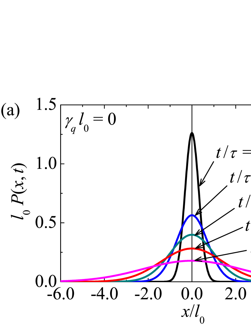
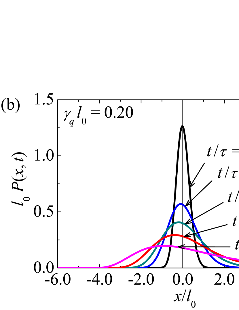
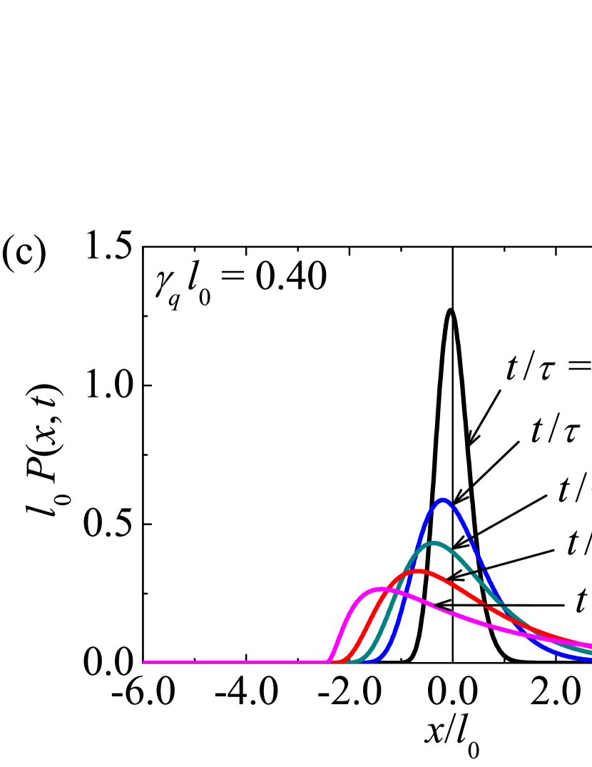
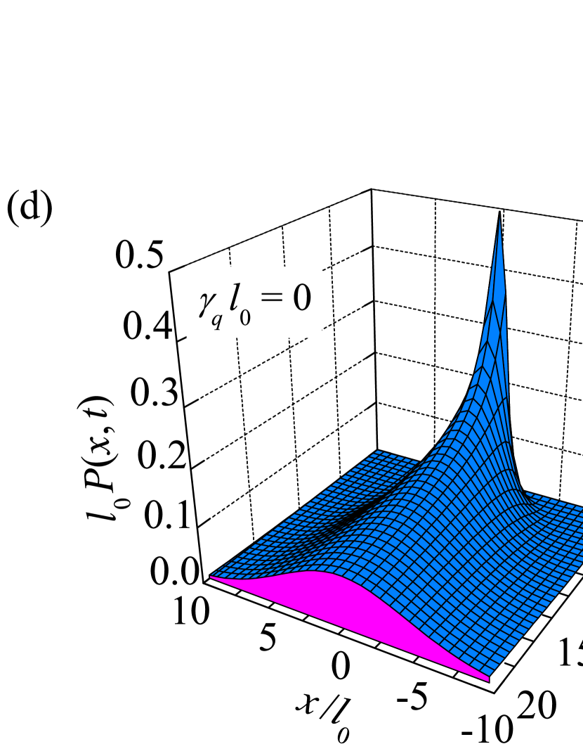
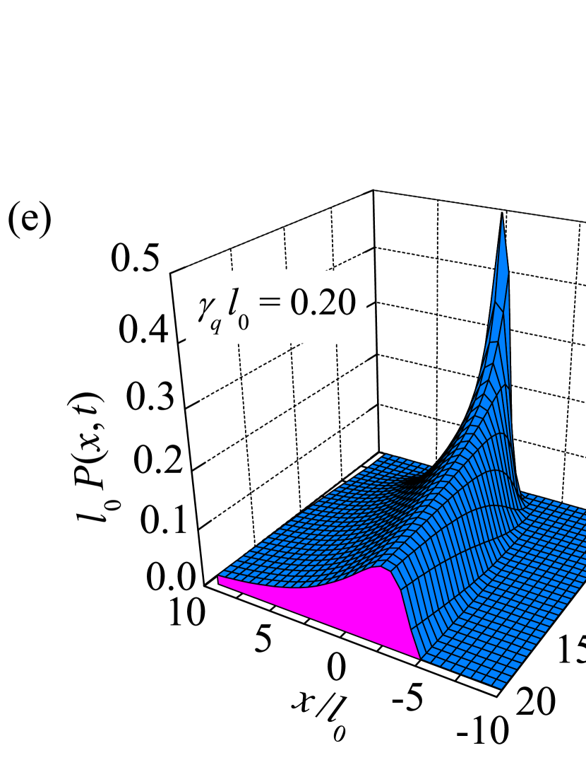
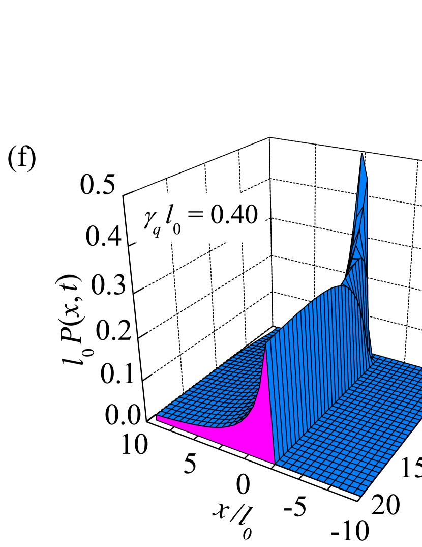
Figure 1: 2D (upper line) and 3D (bottom line) representations of the solutions $P(x,t)$ of the inhomogeneous FPE for free particle with parameters $\gamma_{q}l_{0}=0$ (usual case), $0.2$ and $0.4$. An asymmetry with respect to $x=0$ increases with $\gamma_{q}l_{0}$. The divergence of Eq. (22) for $x\rightarrow x_{\textrm{d}}=-1/\gamma_{q}$ implies a diffusion limited to the interval $x<x_{\textrm{d}}$. Notice that the space and time axis of the 3D plots are inverted (increase from right to left), for a better visualization.

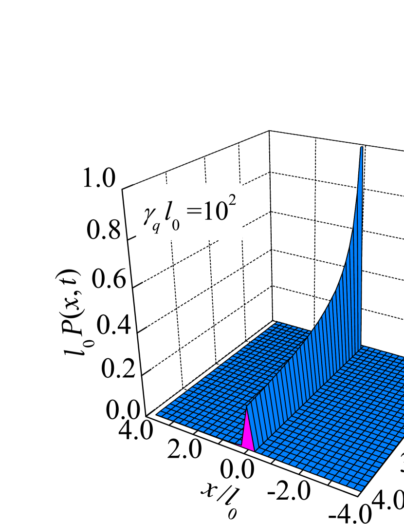
Figure 2: 3D representation of $P(x,t)$ for $\gamma_{q}l_{0}=10^{2}$ showing that diffusion is stopped at $x=0$ for sufficiently high values of $\gamma_{q}l_{0}$ (illustrated with $x_{\textrm{d}}=-10^{-2})$ for a better visualization.

The transformation $x\rightarrow x_{q}$ in equation (92) leads the $n$-th moment of the distribution

$$\langle x^{n}(t)\rangle=\int_{-\infty}^{\infty}x^{n}P(x,t)dx=\int_{-\infty}^{\infty}x^{n}\mathcal{P}_{q}(x,t)d_{q}x$$ (95)

into

$$\langle x^{n}(t)\rangle = \int_{-\infty}^{\infty}\frac{1}{\sqrt{2\pi\Gamma t}}\frac{x^{n}}{1+\gamma_{q}x}\exp\left[-\frac{\ln^{2}(1+\gamma_{q}x)}{(2\Gamma t)\gamma_{q}^{2}}\right]dx$$

$$= \int_{-\infty}^{\infty}\frac{1}{\sqrt{2\pi\Gamma t}}\left(\frac{e^{\gamma_{q}x_{q}}-1}{\gamma_{q}}\right)^{n}e^{-{x}_{q}^{2}/(2\Gamma t)}dx_{q}.$$

The first and second moments are

$$\langle x(t)\rangle = \frac{e^{(\Gamma t)\gamma_{q}^{2}/2}-1}{\gamma_{q}},$$ (96a)

$$\langle x^{2}(t)\rangle = \frac{e^{2(\Gamma t)\gamma_{q}^{2}}-2e^{(\Gamma t)\gamma_{q}^{2}/2}+1}{\gamma_{q}^{2}}.$$ (96b)

Figure 3 shows $\langle(\Delta x)^{2}(t)\rangle$ as a function of time for some values of $\gamma_{q}l_{0}$. The spreading is hyperdiffusive, i.e., faster than the superballistic power-law diffusion, and exponentially increases for $t/\tau\gg 1$, with a characteristic time $\tau=1/(\gamma_{q}^{2}\Gamma)$. The normal diffusion is recovered for $\gamma_{q}\rightarrow 0$, corresponding to an infinite characteristic time $\tau$.

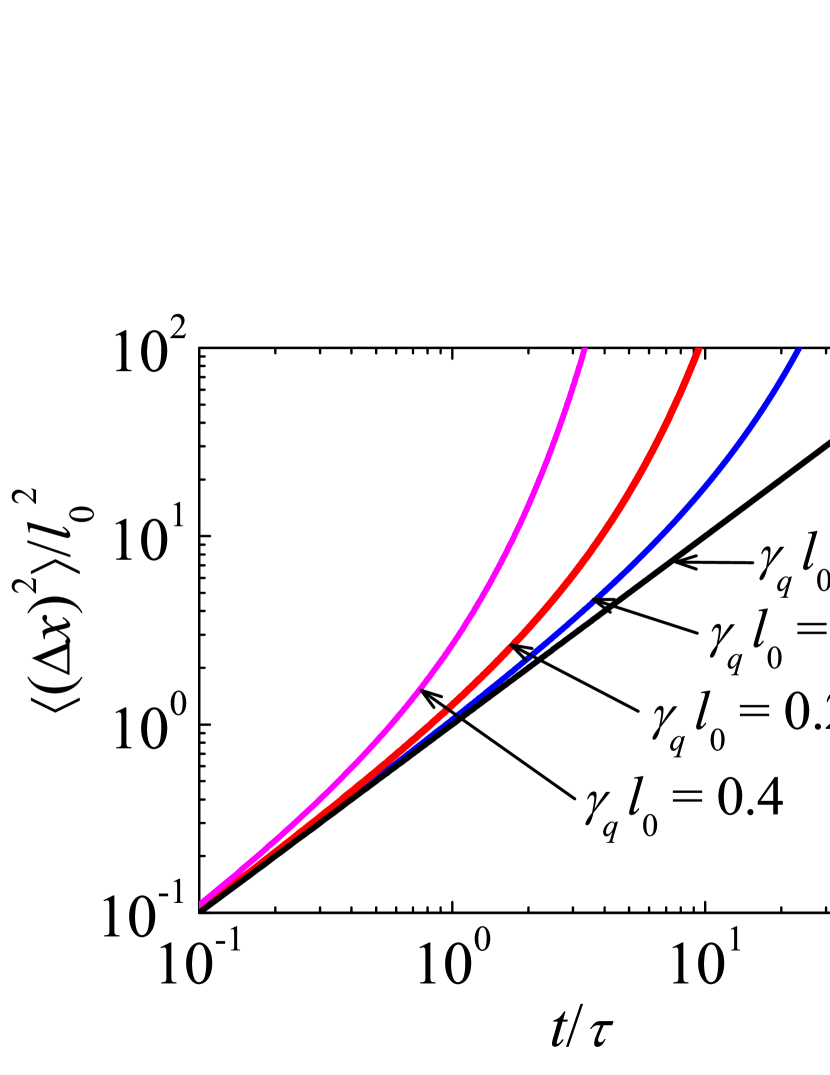
Figure 3: Plot of $\langle(\Delta x)^{2}(t)\rangle=\langle x^{2}(t)\rangle-\langle x(t)\rangle^{2}$ as a function of time for a free particle. Normal diffusion behavior, $\langle(\Delta x)^{2}\rangle\approx\Gamma t$, is observed for $t/\tau\ll 1$, $\forall\gamma_{q}l_{0}$, and exponential hyperdiffusion, $\langle(\Delta x)^{2}\rangle\propto e^{2t/\tau}$, for $t/\tau\gg 1$.

V.2 Confining potential with linear drift coefficient

The $q$-deformed FPE for $A(x)=-\alpha x$ is

$$\frac{\partial\mathcal{P}_{q}(x,t)}{\partial t}=\alpha\mathcal{D}_{q}[x\mathcal{P}_{q}(x,t)]+\frac{\Gamma}{2}\mathcal{D}_{q}^{2}{\mathcal{P}_{q}(x,t)}.$$ (97)

In this case the associated effective potential (81) is given by

$$V_{\textrm{ef}}(x)=\frac{\alpha^{2}}{2\Gamma}x^{2}-\frac{\alpha\gamma_{q}}{2}x-\frac{\alpha}{2}.$$ (98)

The eigenfunctions $\psi_{q}(x)$ for the operator $\hat{\mathcal{K}}_{q}$ (see equation (79)) can be obtained from a comparison with the solutions of the $q$-deformed time-independent Schrödinger equation for a harmonic oscillator with frequency $\omega_{0}$ (for the usual case $q=1$) and electric charge $e$ in a uniform electric field $\vec{\mathcal{E}}=\mathcal{E}\hat{x}$ Nascimento-Ferreira-Aguiar-Guedes-CostaFilho-2018 :

$$-\frac{\hbar^{2}}{2m_{0}}\mathcal{D}_{q}^{2}\psi_{q}+\left(\frac{1}{2}m_{0}\omega_{0}^{2}x^{2}-e\mathcal{E}x+V_{0}\right)\psi_{q}(x)=E\psi_{q}(x),$$ (99)

where $V_{0}$ is a constant. The solutions of equation (99) in absence of an electric field has been studied CostaFilho-Alencar-Skagerstam-AndradeJr-2013 ; Costa-Borges-2018 , the eigenfunctions and energies are obtained by means of a canonical point transformation that maps the system into a Morse oscillator. A similar transformation can be used for $\vec{\mathcal{E}}\neq 0$. From the change of variables $\chi(s)=\psi_{q}(x(s))$ with $s(x)=\gamma_{q}^{-1}\ln[(1+\gamma_{q}x)/(1+\gamma_{q}x_{0})]$ and $x_{0}=e\mathcal{E}/(m_{0}\omega_{0}^{2})$, it follows

$$-\frac{\hbar^{2}}{2m_{0}}\frac{d^{2}{\chi}(s)}{ds^{2}}+\frac{m_{0}\Omega_{q}^{2}}{2\gamma_{q}^{2}}(e^{\gamma_{q}s}-1)^{2}\chi(s)=\widetilde{E}\chi(s).$$ (100)

This equation corresponds to a quantum Morse oscillator with frequency of small oscillations $\Omega_{q}=\omega_{0}(1+\gamma_{q}x_{0})$ around the equilibrium position and energy $\widetilde{E}=E-V_{0}+e^{2}\mathcal{E}^{2}/(2m_{0}\omega_{0}^{2})$. Consequently, the eigenfunctions of equation (99) are

$$\psi_{q,n}(x)=\chi_{n}(s(x))=A_{n}e^{-z(x)/2}[z(x)]^{\nu/2}L_{n}^{(\nu)}(z(x)),$$ (101)

where $z(x)=2d(1+\gamma_{q}x)$, $d=m_{0}\omega_{0}/(\hbar\gamma_{q}^{2})$, $\nu=2d(1+\gamma_{q}x_{0})-1-2n>0$, $A_{n}^{2}=\nu\gamma_{q}n!/(\nu+n)!$, and $L_{n}^{(\nu)}(z)$ are the associated Laguerre polynomials. The energy eigenvalues of the equation (99) are

$$E_{n} = V_{0}-\frac{e^{2}\mathcal{E}^{2}}{2m_{0}\omega_{0}^{2}}+\hbar\omega_{0}\left(1+\frac{\gamma_{q}e\mathcal{E}}{m_{0}\omega_{0}^{2}}\right)\left(n+\frac{1}{2}\right)$$ (102)

$$-\frac{\hbar^{2}\gamma_{q}^{2}}{2m_{0}}\left(n+\frac{1}{2}\right)^{2}.$$

The number of bound states of the deformed oscillator is $N_{b}=\lfloor d(1+\gamma_{q}x_{0})-1/2\rfloor$, $\lfloor u\rfloor$ denoting the floor function, which tends to increase (decrease) for $\gamma_{q}x_{0}>0$ ($\gamma_{q}x_{0}<0$) in the presence of an external electric field. The relations $\hbar^{2}/m_{0}=\Gamma$, $m_{0}\omega_{0}^{2}=\alpha^{2}/\Gamma$, $e\mathcal{E}=\alpha\gamma_{q}/2$, and $V_{0}=-\alpha/2$, lead to

$$\psi_{q,n}(x) = A_{n}e^{-\eta(1+\gamma_{q}x)}\left[2\eta(1+\gamma_{q}x)\right]^{\eta-n}$$ (103)

$$\times L_{n}^{(2\eta-2n)}(2\eta(1+\gamma_{q}x)),$$

where $\eta=\alpha/(\Gamma\gamma_{q}^{2})$ and $A_{n}^{2}=2(\eta-n)\gamma_{q}n!/(2\eta-n)!$. The eigenvalues of $\hat{\mathcal{K}}_{q}$ are

$$\Lambda_{n} = -E_{n}=-\alpha n\left(1-\frac{\Gamma\gamma_{q}^{2}}{2\alpha}n\right),$$ (104)

with $\Lambda_{n}<0$ for all $n\in\mathbb{N}$, except $\Lambda_{0}=0$. The eigenfunctions of (103) are orthogonalized through the deformed inner product $\int_{-\infty}^{+\infty}\psi_{q,n}(x)\psi_{q,n}(x)d_{q}x=\delta_{n,m}$. The coefficients $c_{n}$ of (82) with the initial condition $P(x,0)=\mathcal{P}_{q}(x,0)/(1+\gamma_{q}x)=\delta(x)$ are $c_{n}=\psi_{q,n}(0)/\psi_{q,0}(0)$, so the general solution of equation (97) results

$$\mathcal{P}_{q}(x,t)=\frac{\psi_{q,0}(x)}{\psi_{q,0}(0)}\sum_{n}\psi_{q,n}(x)\psi_{q,n}(0)e^{-t\Lambda_{n}}.$$ (105)

The summation in equation (105) has the form of a quantum propagator for the Morse oscillator Toutounji-2017 , from which we obtain its stationary solution

$$\mathcal{P}_{q}^{(\text{st})}(x)=\frac{\gamma_{q}\left[\frac{1}{\sigma_{0}^{2}{\gamma}_{q}^{2}}(1+\gamma_{q}x)e^{-(1+\gamma_{q}x)}\right]^{\frac{1}{\sigma_{0}^{2}{\gamma}_{q}^{2}}}}{\left(\frac{1}{\sigma_{0}^{2}{\gamma}_{q}^{2}}\right)!},$$ (106)

with $\Gamma/(2\alpha)=\sigma_{0}^{2}$. The transformations $\gamma_{q}\rightarrow-\gamma_{q}$, $x\rightarrow-x$, and $x_{\textrm{d}}\rightarrow-x_{\textrm{d}}$ are equivalent, due to the asymmetry of the diffusion (see Fig. 1), which tends to concentrate the probability density around $x=x_{\textrm{d}}$. Alternatively, the stationary solution can be obtained from (74) using $A(x)=-\alpha x$.

Figure 4(a) shows some plots of the stationary solution $P^{(\text{st})}(x)=\mathcal{P}_{q}^{(\text{st})}(x)/(1+\gamma_{q}x)$ for some values of $\sigma_{0}\gamma_{q}$. For $|\gamma_{q}|\rightarrow 1$ the PDF (106) diverges at $x_{\textrm{d}}=-1/\gamma_{q}$. Figure 4(b) shows the deformed entropy (66) as a function of $\gamma_{q}$ for the stationary PDF along with the entropic contributions of the particles and the medium, obtained by numerical integration. Localization of particles at $x_{\textrm{d}}$ for $\gamma_{q}\sigma_{0}\to 1$ implies $S_{\text{BG}}=-\int P\ln(\bar{\sigma}P)dx\to 0$ with $\bar{\sigma}=e=\text{constant}$. The greater the value of the parameter $\gamma_{q}$, the greater (smaller) is the entropic contribution of the medium (particles) on the total entropy.

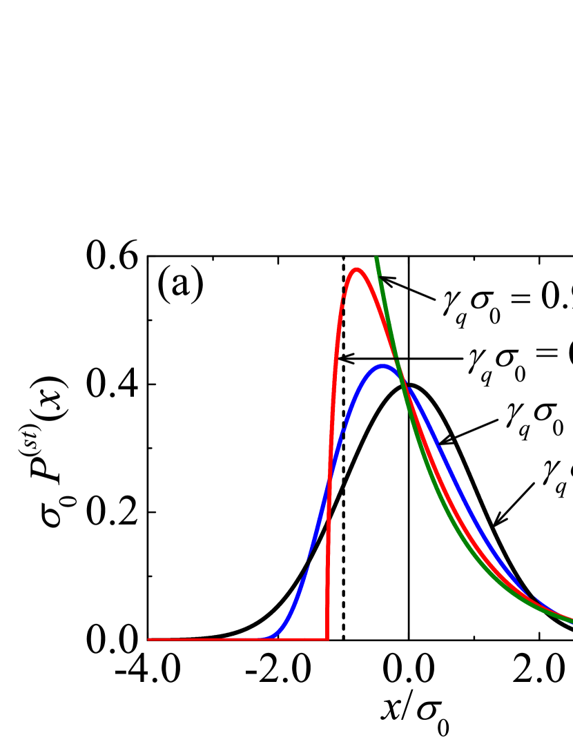
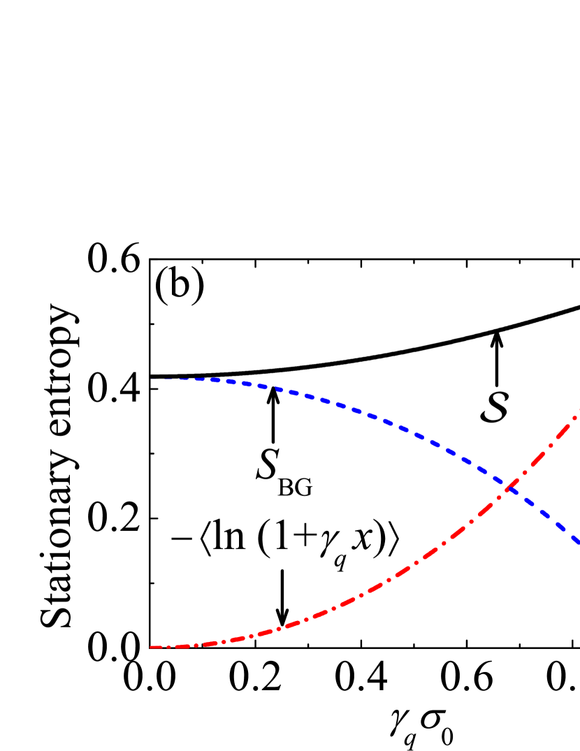
Figure 4: FPE for an inhomogeneous media with a linear potential. (a) Stationary solution for different values of $\sigma_{0}\gamma_{q}$. Similarly to the free particle (see Fig. 1), asymmetry in the PDF is observed. (b) Entropy $\mathcal{S}$ of the system (black line), the contribution of the entropy of the particles $S_{\text{BG}}$ (blue dashed line), and the contribution of the medium, $-\langle\ln(1+\gamma_{q}x)\rangle$, (red dash-dot line), (see Eq. (66)), as a function of the inhomogeneity of the medium, controlled by $\gamma_{q}\sigma_{0}$.

VI Discussion and comparison with the literature

Here follows a discussion of the formalism presented in the light of some literature of inhomogeneous diffusion: the van Kampen’s approach Landauer ; vanKampen-87 ; vanKampen-book and the superstatistics superstatistics ; vanderStraeten . Also, we include two possible fluctuation theorems along with an application of the deformed FPE to anomalous diffusion in optical lattices Lutz ; Beck-entropy .

VI.1 Consistency with van Kampen’s approach

Our aim is to show that the van Kampen’s description of Sub-Section II.2 can be expressed in terms of the deformed Fokker-Planck equation (56) by means of a suitable choice of the deformation $\kappa(x)$ for case in which the functional form of the temperature $T$ and the mobility of the particle $\mu$ are the same:

$$\frac{T(x)}{T_{0}}=\frac{\mu(x)}{\mu_{0}}=\frac{1}{\kappa(x)}$$ (107)

with $T_{0}$ and $\mu_{0}$ their corresponding values in the case of constant temperature and mobility. By simple inspection between the equations (55), (56) and (11), and the deformation $\kappa(x)\equiv h(u)$ in (34) $\mathcal{D}_{[\kappa]}=\frac{1}{\kappa(x)}\frac{d}{dx}$, equation (11) can be rewritten as

$$\frac{\partial\mathcal{P}_{[\kappa]}(x,t)}{\partial t}=\mathcal{D}_{[\kappa]}[\mu_{0}V^{\prime}(x)\mathcal{P}_{[\kappa]}(x,t)]+\mu_{0}T_{0}\mathcal{D}_{[\kappa]}^{2}\mathcal{P}_{[\kappa]}(x,t)$$ (108)

that is the deformed FPE (56) with the identification of the potential drift $A(x)$ and the constant $\Gamma$ as

$$A(x) = -\mu_{0}V^{\prime}(x)$$

$$\Gamma/2 = \mu_{0}T_{0}.$$ (109)

We remark some consequences regarding the connection between the van Kampen’s diffusion equation (11) and the deformed FPE (56). The first one is that the choice (107) implies

$$\beta(x)=\frac{1}{k_{B}T(x)}=\beta_{0}\sqrt{\frac{m(x)}{m_{0}}}.$$ (110)

with $\beta(x)=\beta_{0}$ corresponding to the constant temperature case, thus linking the inverse of the temperature with the position-dependent mass.

Second remark, the entropic density $s_{[\kappa]}(P)=-\frac{P}{\kappa}\ln\left(\frac{P}{\kappa}\right)$ satisfies $\frac{d^{2}s_{[\kappa]}}{dP^{2}}=-\frac{1}{\kappa P}<0$ and since the deformed stationary solution $\mathcal{P}^{(\textrm{st})}(x)=\kappa(x)P^{(\textrm{st})}(x)$ maximizes $\mathcal{S}$ then $P^{(\textrm{st})}(x)$ (Section V.2) also maximizes

$$\mathcal{S}=S_{\textrm{BG}}-\langle\ln[T(x)/T_{0}]\rangle$$ (111)

The expression (111) represents an entropy functional for the existence of the deformed $H$-theorem (Sub-Section III.3) in an inhomogeneous medium with a position-dependent temperature $T(x)$. The first term of Equation (111) has a microscopic nature (the probability density function), while its second term depends on a macroscopic variable. This would be considered as an inconsistency within the usual statistical mechanics framework, but within the superstatistics context, the second term is an average over a continuous of canonical ensembles of temperatures $T(x)$. The confining potential with linear drift of Sub-Section V.2 exemplifies this point. In the context of the van Kampen’s equation (11) this case corresponds to an inhomogeneous media with a linear temperature profile given by equations (68) and (107) and a external force $-V^{\prime}(x)=-\frac{\alpha}{\mu_{0}}x$ ($A(x)=-\alpha x$) with $\alpha,\mu_{0}\geq 0$. Figure 4(b) shows the increase of the entropy $\mathcal{S}$ with the growth rate of the temperature $\frac{1}{T_{0}}\frac{dT}{dx}=\gamma_{q}$, $S_{\textrm{BG}}$, decreases, but the contribution of the medium sufficiently compensates, and $\mathcal{S}$ increases with the inhomogeneity of the temperature.

Finally, if $T(x)/\mu(x)\neq\textrm{constant}$, equation (11) can be expressed by means of deformed derivatives. In fact, using that $\mathcal{P}_{[1/\mu]}(x,t)=P(x,t)\mu(x)/\mu_{0}$, $\mathcal{P}_{[1/T]}(x,t)=P(x,t)T(x)/T_{0}$ and $\mathcal{D}_{[1/\mu]}=\frac{\mu(x)}{\mu_{0}}\frac{d}{dx}$, $\mathcal{D}_{[1/T]}=\frac{T(x)}{T_{0}}\frac{d}{dx}$, the van Kampen’s diffusion equation (11) is written as

$$\frac{\partial\mathcal{P}_{[1/\mu]}(x,t)}{\partial t} = \mathcal{D}_{[1/\mu]}[\mu_{0}V^{\prime}(x)\mathcal{P}_{[1/\mu]}(x,t)]$$ (112)

$$+\mu_{0}T_{0}\mathcal{D}_{[1/\mu]}^{2}[\mathcal{P}_{[1/T]}(x,t)].$$

The general solution of this equation is beyond the scope of the this work.

VI.2 Superstatistics and position-dependent mass Langevin equations

A deep connection between the position-dependent Langevin equation (46) and the superstatistics version (13a) can be given by considering $\lambda(x)=\lambda_{0}$ and multiply the left and right sides of (46) by $\dot{x}$, then we obtain

$$\frac{d}{dt}\left(\frac{1}{2}m(x)\dot{x}^{2}\right)=-m(x)\lambda_{0}\dot{x}^{2}+(F(x)+R(t))\dot{x}.$$ (113)

By means of the change of variable

$$x_{[\kappa]}(x)=\int^{x}\sqrt{\frac{m(x^{\prime})}{m_{0}}}dx^{\prime}$$ (114)

the equation (113) can be rewritten as

$$\frac{d{v}_{[\kappa]}}{dt}=-\lambda_{0}v_{[\kappa]}+\frac{\overline{F}(x_{[\kappa]})}{m_{0}}+\sqrt{\frac{2\lambda_{0}}{m_{0}\beta(x_{[\kappa]})}}\overline{\xi}(t),$$ (115a)

$$\frac{dx_{[{\kappa}]}}{dt}=v_{[{\kappa}]}$$ (115b)

with

$$\overline{F}(x_{[\kappa]})=F(x(x_{[\kappa]}))\sqrt{\frac{m_{0}}{m(x(x_{[\kappa]}))}}=-\frac{dV(x(x_{[\kappa]}))}{dx_{[\kappa]}},$$ (116a)

$$\beta(x_{[\kappa]})=\beta_{0}\frac{m(x(x_{[\kappa]}))}{m_{0}}=\beta_{0}\kappa^{2}(x(x_{[\kappa]})),$$ (116b)

$$\overline{\xi}(t)=\sqrt{\frac{m_{0}\beta_{0}}{2\lambda_{0}}}R(t)$$ (116c)

where $\beta_{0}$ denotes the standard case $\beta(x_{[\kappa]})=\textrm{constant}$. The set of equations (115a) is formally identical to (13a), thus giving a demonstration by first principles of the superstatistics Langevin equation in terms of a position-dependent mass particle.

The stationary solutions of the superstatistics (15) and of the deformed FPE (III.2) along with the relationship $\beta(x)=1/\kappa(x)$ from (110) indicate they are the same distribution. Moreover, from the deformed stationary solution of the confining potential (106), the equation (55) and by the same procedure for obtaining the velocity distribution (vanderStraeten , equation (16)) in the overdamped limit, we obtain the distribution $f(\beta_{q})$ for the $q$-deformation $\beta_{q}(x)=\frac{1}{1+\gamma_{q}x}$

$$f({\beta}_{q})=\frac{\beta_{q}^{-\alpha-1}}{\Gamma(\alpha)}\exp\left(-\frac{\theta}{\beta_{q}}\right),\quad\alpha=\theta=\frac{1}{\sigma_{0}^{2}\gamma_{q}^{2}},$$ (117)

which is the inverse Gamma distribution of the example $\beta(x)=\frac{1}{|x|+a}$ of vanderStraeten in the limit $a\rightarrow 0$. Also, from $\beta_{q}(x)$ other candidate for the force $\frac{2}{\Gamma}A(x)$ can be obtained by means of equation (18) of vanderStraeten .

Position-dependent mass and superstatistical Langevin equations (in $x$ and $y$ spaces respectively) (46) and (115a), are equivalent, maintaining the position and the velocity at the same status level, from which results the overdamped PDM Langevin equation (47) (or equivalently (48)), in $x$ for $\lambda(x)\gg\tau^{-1}$. Analogously, the van Kampen’s FPE (11) is not equivalent to the superstatistical Langevin equation (13a), since the overdamped limit has not been taken in the latter.

VI.3 Work fluctuation theorems for position-dependent mass particle

We outline two possible fluctuation theorems (FT) Kubo-1966 ; FDT-Beck in a position-dependent mass scenario by reviewing some works on fluctuation theorems for a dragged Brownian particle FT-Wang ; FT-Cohen . For simplicity we restrict our discussion to the deformation (68). In order to apply the FT theorem FT-Cohen and inspired by the experiment of Wang, we consider a one-dimensional Brownian particle of constant mass $m_{0}$ in a medium of friction $\lambda_{0}$ and temperature $T_{0}$ in the deformed frame $x_{q}$ (93), and subjected to a force $F(x_{q},{x}^{*}_{q}(t))=-k(x_{q}-{x}^{*}_{q}(t))$ with an arbitrary time-dependent position $x^{*}(t)$. Let us denote $W_{\tau}$ and $\overline{W}_{\tau}$ the works done on the system during a time $\tau$, with $\tau$ the time scale of the fluctuations in the spaces $x$ and $x_{q}$ respectively. By means of the transformation (93) it is immediate to show that the overdamped position-dependent mass Langevin equation (47) is equivalent to

$$\dot{x}_{q}=-\frac{x_{q}-{x}^{*}_{q}(t)}{\tau_{r}}+\xi(t)$$ (118)

with $\tau_{r}=\lambda_{0}/k$ the relaxation time, $\langle\xi(t)\rangle=0$ and $\langle\xi(t)\xi(t^{\prime})\rangle=2k_{B}T_{0}\lambda_{0}\delta(t-t^{\prime})$ and a force $F(x,x^{*}(t))=(1/\gamma_{q})\ln((1+\gamma_{q}x)/(1+\gamma_{q}x^{*}(t)))$. Under these conditions, from (118) the work FT of the equation (31) of FT-Cohen in the space $x_{q}$ follows

$$\frac{P(\overline{W}_{\tau})}{P(-\overline{W}_{\tau})}=e^{\overline{W}_{\tau}},$$ (119)

with $P(\overline{W}_{\tau})$ the probability distribution of $\overline{W}_{\tau}$, constructed by measuring $\overline{W}_{\tau}$ over time intervals $\tau$ FT-Wang . By the definition of equation (5) of FT-Cohen ,

$$\overline{W}_{\tau} = \beta_{0}\int_{0}^{\tau}dt\;{v}_{q}^{*}(t)\;[-k(x_{q}(t)-x_{q}^{*}(t))]$$ (120)

$$= \beta_{0}\int_{0}^{\tau}dt\;\frac{v^{*}(t)}{1+\gamma_{q}x^{*}(t)}\;F(x(t),x^{*}(t))$$

$$= \langle W_{\tau}\rangle_{q},$$

with ${v}_{q}=v/(1+\gamma_{q}x)$. The probability of the work done must be the same on both spaces $x$ and $x_{q}$, so $P(W_{\tau})dW_{\tau}=P(\overline{W}_{\tau})d\overline{W}_{\tau}$, from which follows $P(\overline{W}_{\tau})/P(-\overline{W}_{\tau})=P(W_{\tau})/P(-W_{\tau})$. Then, from (120) we recast the work FT (119) in standard space $x$,

$$\frac{P(W_{\tau})}{P(-W_{\tau})}=e^{\langle W_{\tau}\rangle_{q}},$$ (121)

that constitutes a first version of the work FT FT-Cohen with $W_{\tau}$ averaged by the deformation (68). We can provide a second (stationary state) version of the work FT, now by measuring the ratio $P(W_{\tau})/P(-W_{\tau})$ over single trajectories in a stationary state of the type (15), that is, by dividing a stationary trajectory of total time $t$ in a sequence of $M\gg 1$ time intervals with duration $\tau$ ($t_{i+1}-t_{i}=\tau$) and initial times $t_{1},\ldots,t_{M}$ FT-Cohen . This corresponds to the stationary state fluctuation theorem (SSFT) FT-Cohen , as a case of the FT in the long term regime $t\gg\tau$. For the constant velocity case, $v^{*}(t)=v_{0}$ of $x^{*}(t)$ FT-Wang ; FT-Cohen , it follows the time scale $\tau_{L}=1/(\gamma_{q}v_{0})$, during which the deformation (68) varies. The time scales ordering $\tau<\tau_{L}\ll t$ implies the factor $1/(1+\gamma_{q}x^{*}(t))$ in (120) is approximately constant, so from (121) we obtain

$$\frac{P(W_{\tau})}{P(-W_{\tau})}=e^{\beta(x^{*}(t_{0}))W_{\tau}}$$ (122a)

$$\beta(x^{*}(t_{0}))=\beta_{0}/(1+\gamma_{q}x^{*}(t_{0}))$$ (122b)

with $t_{0}\in(0,\tau)$, that can be considered a manifestation of the superstatistics work FT of FDT-Beck linked with position-dependent mass systems, where we have used the identification (110). Employing (122) we can derive an expression for the expectation of the ratio $P(W_{\tau})/P(-W_{\tau})$ for the inverse Gamma distribution (117) of the confining potential case. Over a stationary trajectory in the long term regime, by averaging (122) with (117) we obtain

$$\left\langle\frac{P(-W_{\tau})}{P(W_{\tau})}\right\rangle=\frac{2}{\Gamma(\alpha)}(\alpha W_{\tau})^{\alpha/2}K_{\alpha}(2\sqrt{\alpha W_{\tau}}),$$ (123)

with $\alpha=1/(\sigma_{0}^{2}\gamma_{q}^{2})$ and $K_{\nu}(x)$ is the modified Bessel function of the second kind. The average of the probability ratio (123) asymptotically decays as a power law $W_{\tau}^{-\alpha/2}$ for small values of $W_{\tau}$, while for large $W_{\tau}$, it decays exponentially as if there were no $\beta$ fluctuations. We could extrapolate the validity of the FT for a Morse potential force, that is, by making the substitution $-(1/\gamma_{q})[\exp(\gamma_{q}(x_{q}-x_{q}^{*}))-1]$ $\rightarrow$ $(x_{q}-x_{q}^{*})$ in (118) with a relaxation time $\tau_{r}=\lambda_{0}\gamma_{q}/D$ and $D$ the dissociation constant of the Morse potential. In the long term regime, the confining potential decays as a power law or as an exponential, for small or large $W_{\tau}$, respectively. This behavior follows from (123), along the same steps that lead to (122). A possible test for equation (123) is the experiment referred to in Ref. FT-Wang in the long term regime with temperature and mobility profiles given by equations (68) and (107), together with the condition $\tau_{L}=1/(\gamma_{q}v_{0})>\tau$.

VI.4 Anomalous diffusion in optical lattices

Other important case of inhomogeneous diffusion has been investigated in optical lattices Lutz , whose relevance against others counterparts lies in the fact that its optical periodic potential is completely known, thus allowing to control it in a precise way. In this regard, an intermediate atomic transport regime can be identified, between diffusive motion and ballistic motion, in which anomalous diffusion occurs and the dynamics is adequately described by nonextensive statistics Lutz ; Beck-entropy . In this regime, the atom–laser interaction in the optical lattice is governed by a quantum master equation whose spatial averaging gives the Rayleigh equation for the Wigner function $W(p,t)$,

$$\frac{\partial W(p,t)}{\partial t}=-\frac{\partial}{\partial p}[K(p)W(p,t)]+\frac{\partial}{\partial p}\left[D(p)\frac{\partial W(p,t)}{\partial p}\right],$$ (124)

where the functions $K(p)$ and $D(p)$ are the drift (cooling force, the Sisyphus effect) and diffusion (stochastic momentum fluctuations of $p$) coefficients. Our purpose is to show that Rayleigh equation (124) can also be expressed as a particular deformed FPE (56) for the stationary case $\frac{\partial W(p,t)}{\partial t}=0$. Noticing that the diffusion coefficient $D(p)$ defines the deformed derivative (see (34) with $h(u)\equiv 1/D(p)$) $\mathcal{D}_{1/D}=\frac{D(p)}{D_{0}}\frac{\partial}{\partial p}$ (with $D_{0}$ corresponding to fluctuations of photon emissions Lutz ) and by making $W(p,t)=\overline{W}(x,p)D(p)$, then $W(p,t)$ can be interpreted as a deformed version of $\overline{W}(x,p)$, i.e., $W(p,t)=\mathcal{\overline{W}}_{[1/D]}(x,p)$ (according to (55)). Thus, we recast (124) for the stationary case as

$$0=-\mathcal{D}_{[1/D]}[K(p)\mathcal{\overline{W}}_{[1/D]}(p)]+D_{0}\mathcal{D}_{[1/D]}^{2}\mathcal{\overline{W}}_{[1/D]}(p),$$ (125)

which is entirely expressed in the deformed space $d_{[1/D]}p=\frac{D_{0}}{D(p)}dp$ with constant diffusion coefficient $D_{0}$. Moreover, it follows from (58) its stationary solution,

$$W^{(\textrm{st})}(p) = \mathcal{\overline{W}}_{[1/D]}^{(\textrm{st})}(p)$$ (126)

$$= C\exp\left(\frac{1}{D_{0}}\int^{p}K(p^{\prime})d_{[1/D]}p^{\prime}\right)$$

$$= C\left[1-\beta(1-q)p^{2}\right]^{1/(1-q)},$$

which is the Tsallis distribution (equation (5) of Lutz ), with $K(p)/D(p)=\frac{2\beta p}{1-\beta(1-q)(p)^{2}}$.

VII Conclusions

Table 1: Linear and nonlinear deformed Fokker-Planck and Schrödinger equations.

	deformed derivative	deformed Fokker-Planck equation	deformed Schrödinger equation
Linear	$\displaystyle\mathcal{D}_{q}f(u)=[1+(1-q)u]\frac{df}{du}$	$\displaystyle\begin{array}[]{rcl}\displaystyle\frac{\partial\mathcal{P}_{q}(x,t)}{\partial t}&=&-\mathcal{D}_{q,x}[A(x)\mathcal{P}_{q}(x,t)]\\ &&\displaystyle+\frac{\Gamma}{2}\mathcal{D}_{q,x}^{2}\mathcal{P}_{q}(x,t)\end{array}$	$\begin{array}[]{rcl}\displaystyle i\hbar\frac{\partial\Psi_{q}(x,t)}{\partial t}&=&\displaystyle-\frac{\hbar^{2}}{2m_{0}}\mathcal{D}_{q,x}^{2}\Psi_{q}(x,t)\\ &&+V(x)\Psi_{q}(x,t)\end{array}$
	(Eq. (19))	(Eq. (69), proposed in this work)	(Eq. (23), proposed in CostaFilho-Almeida-Farias-AndradeJr-2011 )
Nonlinear	$\displaystyle\widetilde{\mathfrak{D}}_{q}f(u)=[f(u)]^{1-q}\frac{df}{du}$	$\displaystyle\begin{array}[]{rcl}\displaystyle\widetilde{{\mathfrak{D}}}_{q,t}P_{q}(x,t)&=&-\widetilde{{\mathfrak{D}}}_{q,x}[A(x)P_{q}(x,t)]\\ &&\displaystyle+\frac{\Gamma}{2}\widetilde{{\mathfrak{D}}}_{q,x}^{2}P_{q}(x,t)\end{array}$	$\begin{array}[]{rcl}\displaystyle i\hbar\widetilde{{\mathfrak{D}}}_{q,t}\Phi_{q}(x,t)&=&\displaystyle-\frac{\hbar^{2}}{2m_{0}}\widetilde{{\mathfrak{D}}}_{q,x}^{2}\Phi_{q}(x,t)\\ &&+V(x)\Phi_{q}(x,t)\end{array}$
	(Eq. (24))	(Eq. (31), proposed in Plastino-Plastino-1995 )	(Eq. (33), proposed in Nobre-RegoMonteiro-Tsallis-2011 )

Quantum and classical formalisms properly deformed to account for systems with position-dependent effective mass recently addressed in the literature CostaFilho-Almeida-Farias-AndradeJr-2011 ; CostaFilho-Alencar-Skagerstam-AndradeJr-2013 ; Costa-Borges-2014 ; Costa-Borges-2018 ; Costa-Gomez-2018 ; Nascimento-Ferreira-Aguiar-Guedes-CostaFilho-2018 have been studied for which derivative operators are replaced by their deformed forms. Table I displays the whole picture, exhibiting deformed versions of Fokker-Planck and Schrödinger equations, and the gap fulfilled by the present work. The linearity and the nonlinearity of the equations are rephrased by linear and nonlinear versions of deformed derivatives. We summarize our contributions as follows.

(i) Two deformed derivatives have been generalized into a unified framework within an arbitrary deformation space $h(x)$, Eqs. (34) and (35). This scenario allows to obtain a linear deformed Fokker-Planck equation that is equivalent to the corresponding FPE in an inhomogeneous media with a position-dependent mass along with dumping and diffusion coefficients as a function of the employed deformation.

(ii) The deformation carries pieces of information about the inhomogeneity of the medium, as a consequence of the equivalence between the FPE in an inhomogeneous medium with position-dependent mass and a deformed FPE in a homogeneous medium with constant mass.

(iii) There is a connection between the molecular and the macroscopic (diffusion) deformed descriptions, given by the Langevin (48) and the Fokker-Planck (69) equations, respectively. Within the macroscopical approach, the diffusion equation (FPE) is written in terms of a deformed linear derivative, while the microscopical approach, the equations of motion (Langevin), uses the corresponding dual deformed nonlinear derivative. This is in complete analogy with the interplay, reported previously in Costa-Borges-2014 ; Costa-Borges-2018 , between the deformed versions of the Schrödinger equation and of the Newton’s law obtained in the classical limit.

(iv) The deformed FPE (56) and the position-dependent mass Langevin equation (47) result equivalent to the nonlinear Langevin equation (44b), thus guaranteeing the existence of a well-defined stationary solution, which satisfies the deformed $H$-theorem of Section V.2, and showing a connection between the standard inhomogeneous diffusion and the one that emerges from a position-dependent mass system.

(v) The entropy of the system (66) is written as the sum of contributions, one from the particles and one from the medium, with the latter increasing with deformation, as illustrated for the case of the confining potential (Figure 4). In the context of the van Kampen’s diffusion equation (11) the entropy contribution of the medium is given in terms of the position-dependent temperature (equation (111)). For the case of the confining potential and the deformation (68), the temperature results linear and with the same inverse Gamma distribution for $f(\beta)$ as in vanderStraeten .

(vi) The solution of the deformed linear FPE for a confining potential can be obtained from an analogy with the corresponding deformed linear Schrödinger equation (Section IV.2).

(vii) Exponential hyper-diffusion is found for times longer than the characteristic time, according to the position-dependent mass, and, consequently, to the deformation parameter, Eq. (96b).

(viii) Instances addressed in Section VI point out the potential use of the deformed FPE in different contexts. Consistency with the van Kampen’s inhomogenous diffusion has been established for the case in which the temperature and the mobility are proportional, while the position-dependent Langevin equation (46) in a deformed space and the superstatistics version of the Langevin equation (13a) are equivalent. Two possible realizations of the work fluctuation theorem has been linked with the diffusion of a position-dependent mass particle, one of them by averaging the work with the deformation (68) while the other was obtained in terms of the superstatistics approach in the long term regime. For the latter we have proposed a modification of the experiment of Wang by suggesting to employ a temperature and mobility profiles $T(x)/T_{0}=\mu(x)/\mu_{0}=(1+\gamma_{q}x)$, in order test power law and exponential decays in the expectation value of the probability work ratio (123) for small and large values of the work $W_{\tau}$ respectively. In the general case the van Kampen’s equation (11) can be expressed by (112) in terms of a mixture of deformations given by the temperature and the mobility. The van Kampen’s FPE along with the superstatistics FPE and the deformed FPE have the same stationary solution and satisfy the relationships given by the Table II.

Table 2: Structure of the inhomogeneous diffusion of the van Kampen’s approach, the superstatistics FPE and the deformed FPE in the position-dependent mass context.

deformed FPE (56) with (107)	$\leftrightarrow$	van Kampen FPE (11)
PDM Langevin equation (46) in $y(x)$ (114)	$\leftrightarrow$	superstatistics Langevin Eq. (13a) in $y(x)$ (114)
deformed FPE (56)	$\nleftrightarrow$	superstatistics FPE (14)
superstatistics FPE (14) with $T(x)=1/\beta(x)$ and $\mu(x)=\mu_{0}$	$\leftrightarrow$	van Kampen FPE (11)

Regarding the anomalous diffusion in optical lattices, the Rayleigh equation for the stationary Wigner function Lutz can be expressed as a deformed FPE in a deformed momentum space $p_{[1/D]}$, with $D(p)$ the diffusion coefficient.

There is an equivalence between the deformed space of the position-dependent mass system, the heterogeneity of the environment and the superstatistics, which could potentially be used to study problems in these areas.

Table I uses the two deformed derivatives (one linear and one nonlinear) for which the $q$-exponential is the eigenfunction. In order to complete the scheme, it is still missing the development of deformed versions of FPE and Schödinger equation using their dual derivatives, i.e., those whose the deformed derivative of the $q$-logarithm of $u$ is $1/u$: $\widetilde{\mathcal{D}}_{q}f(u)$ (Eq. (20)) and $\mathfrak{D}_{q}f(u)$, (Eq. (25)).

The linear deformation of the FPE addressed in this paper does not formally departs from Boltzmann-Gibbs statistical mechanics, within the deformed space (see Eqs. (65), (66)). It is interesting to explore the consequences of nonlinear deformations to identify which case leads to a nonextensive statistical mechanics scenario described by $S_{q}$ entropy. Besides, other deformed algebras could be employed, for instance within the context of relativistic statistical mechanics Kaniadakis-2002 as well as those from entropic information generalizations Beck-entropy ; Rodriguez-2019 , thus leading to different deformations of the FPE.

- (1) P. Langevin, C. R. Acad. Sci. Paris. 146, 530 (1908).
- (2) H. Risken, The Fokker-Planck Equation: Methods of Solution and Applications (Springer, Berlin, 1989).
- (3) H. Scher and E. W. Montroll, Phys. Rev. B 12, 2455 (1975).
- (4) A. R. Plastino and A. Plastino, Physica A 222, 347 (1995).
- (5) C. Tsallis and D. J. Bukman, Phys. Rev. E 54, R2197 (1996).
- (6) L. Borland, Phys. Rev. E 57, 6634 (1998).
- (7) L. Borland, Phys. Lett. A 245, 67-72 (1998).
- (8) R. G. DeVoe, Phys. Rev. Lett. 102, 063001 (2009).
- (9) T. D. Frank, Nonlinear Fokker-Planck Equations: Fundamentals and Applications (Springer, Berlin, 2005).
- (10) M. Muskat, The Flow of Homogeneous Fluids Through Porous Media (McGraw-Hill, New York, 1937).
- (11) A. Klemm, H.-P. Müller, and R. Kimmich, Phys. Rev. E 55, 4413 (1997).
- (12) P. Barrozo, A. A. Moreira, J. A. Aguiar, and J. S. Andrade, Jr., Phys. Rev. B 80, 104513 (2009).
- (13) C. Tsallis, J. Stat. Phys. 52, 479 (1988).
- (14) C. Tsallis, Introduction to Nonextensive Statistical Mechanics (Springer, New York, 2009).
- (15) J. S. Andrade, Jr., G. F. T. da Silva, A. A. Moreira, F. D. Nobre, and E. M. F. Curado, Phys. Rev. Lett. 105, 260601 (2010).
- (16) K. Hizanidis, Phys. Fluids B 1, 675 (1989).
- (17) S. Jang, J. Chem. Phys. 144, 214102 (2016).
- (18) N. Suciu, F. A. Radu, S. Attinger, L. Schüler, and P. Knabner, J. Comput. Appl. Math. 289, 241 (2015).
- (19) B. S. Collyer, C. Connaughton, and D. A. Lockerby, J. Comp. Phys. 325, 116 (2016).
- (20) A. Grassi and A. Raudino, Physica A 395, 171 (2014).
- (21) M. A. F. dos Santos and I. S. Gomez, J. Stat. Mech. 12, 123205 (2018).
- (22) W. Xu et al., Int. J. Heat Mass Tra. 139, 39 (2019).
- (23) T. D. Frank and A. Daffertshofer, Physica A 295, 455 (2001).
- (24) V. Schwammle, E. M. F. Curado, and F. D. Nobre, Eur. Phys. J. B 70, 107 (2009).
- (25) M. S. Ribeiro, F. D. Nobre, and E. M. F. Curado, Entropy 13, 1928 (2011).
- (26) G. Sicuro, P. Rapčan and C. Tsallis, Phys. Rev. E 94, 062117 (2016).
- (27) L. Nivanen, A. Le Méhauté, and Q. A. Wang, Rep. Math. Phys 52, 437 (2003).
- (28) E. P. Borges, Physica A 340, 95 (2004).
- (29) C. Tsallis, Quimica Nova 17, 468 (1994).
- (30) T. C. P. Lobao, P. G. S. Cardoso, S. T. R. Pinho, and E. P. Borges, Braz. J. Phys. 39, 402 (2009).
- (31) P. Tempesta, Phys. Rev. E 84, 021121 (2011).
- (32) G. Bastard, J. K. Furdyna and J. Mycielsky, Phys. Rev. B 12, 4356 (1975).
- (33) O. von Roos, Phys. Rev. B 27, 7547 (1983).
- (34) R. N. Costa Filho, M. P. Almeida, G. A. Farias, and J. S. Andrade Jr., Phys. Rev. A 84, 050102(R) (2011).
- (35) R. N. Costa Filho, G. Alencar, B.-S. Skagerstam, and J. S. Andrade Jr., Europhys. Lett. 101, 10009 (2013).
- (36) E. G. Barbagiovanni and R. N. Costa Filho, Physica E 63, 14 (2014).
- (37) B. G. da Costa and E. P. Borges, J. Math. Phys. 55, 062105 (2014).
- (38) B. G. da Costa and E. P. Borges, J. Math. Phys. 59, 042101 (2018).
- (39) B. G. da Costa and I. S. Gomez, Phys. Lett. A 382, 2605 (2018).
- (40) J. P. G. Nascimento, F. A. P. Ferreira, V. Aguiar, I. Guedes, and R. N. Costa Filho, Physica A 499, 250 (2018).
- (41) B. G. da Costa, I. S. Gomez and M. A. F. dos Santos, EPL 129, 10003 (2020).
- (42) K. Bencheikh, K. Berkane and S. Bouizane, J. Phys. A: Math. Gen. 37 (45), 10719 (2004).
- (43) M.V. Ioffe, E.V. Kolevatova and D.N. Nishnianidze, Phys. Lett. A 380, 3349 (2016).
- (44) M. Alimohammadi, H. Hassanabadi and S. Zare, Nucl. Phys. A 960, 78 (2017).
- (45) K. Li, K. Guo, X. Jiang and M. Hu, Optik 132, 375 (2017).
- (46) Z. Algadhi and O. Mustafa, Ann. Phys. 418, 168185 (2020).
- (47) N. G. van Kampen, Z. Phys. B Condensed Matter 68, 135 (1987).
- (48) N. G. van Kampen, Stochastic Processes in Physics and Chemistry (Elsevier, North Holland, 2007).
- (49) R. Landauer, Phys. Rev. A 12, 636 (1975).
- (50) C. Beck and E. G. D. Cohen, Physica A 322, 267 (2003).
- (51) E. van Der Straeten and C. Beck, Chin. Sci. Bull. 56, 3633 (2011).
- (52) C. Beck, Contemporary Physics 50, 495 (2009).
- (53) E. Lutz, Phys. Rev. A 67, 051402(R) (2003).
- (54) F. D. Nobre, M. A. Rego-Monteiro, and C. Tsallis, Phys. Rev. Lett. 106, 140601 (2011).
- (55) W. Rosa and J. Weberszpil, Chaos, Solitons & Fractals 117, 137 (2018).
- (56) M. A. Rego-Monteiro, Phys. Lett. A 384, (6), 126132 (2020).
- (57) A. O. Caldeira and A. J. Leggett, Physica 121 A, 587 (1983).
- (58) F. Illuminati, M. Patriarca and P. Sodano, Physica A 211, 449 (1994).
- (59) S. Kullback and R. A. Leibler, Ann. Math. Stat. 22, 79 (1951).
- (60) M. T. Araujo and E. Drigo Filho, J. Stat. Phys. 146, 610 (2012).
- (61) M. Toutounji, Ann. Phys. 377, 210 (2017).
- (62) R. Kubo, Rep. Prog. Phys. 29, 255 (1966).
- (63) C. Beck and E. G. D. Cohen, Physica A 344, 393-402 (2004).
- (64) G. M. Wang, E. M. Sevick, E. Mittag, D. J. Searles, and D. J. Evans, Phys. Rev. Lett. 89(5), 050601 (2002).
- (65) R. van Zon and E. G. D. Cohen, Phys. Rev. E 67, 046102 (2003).
- (66) G. Kaniadakis, Phys. Rev. E 66, 056125 (2002).
- (67) M. Rodriguez, A. Romaniega and P. Tempesta, Proc. R. Soc. A 475, 20180633 (2019).