Performance of Hierarchical Sparse Detectors for Massive MTC

Abstract

Recently, a new class of so-called hierarchical thresholding algorithms was introduced to optimally exploit the sparsity structure in joint user activity and channel detection problems. In this paper, we take a closer look at the user detection performance of such algorithms under noise and relate its performance to the classical block correlation detector with orthogonal signatures. More specifically, we derive a lower bound for the diversity order which, under suitable choice of the signatures, equals that of the block correlation detector. Surprisingly, in specific parameter settings non-orthogonal pilots, i.e. pilots where (cyclically) shifted versions interfere with each other, outperform the block correlation detector. Altogether, we show that, in wide parameter regimes, the hierarchical thresholding detectors behave like the classical correlator with improved detection performance but operate with much less required pilot subcarriers. We provide mathematically rigorous and easy to handle formulas for numerical evaluations and system design. Finally, we evaluate our findings with numerical examples and show that, in a practical parameter setting, a classical pilot channel can accommodate up to three advanced pilot channels with the same performance.

I Introduction

Compressed Sensing (CS) is a mathematical field with applications in many engineering disciplines involving big data processing. One of the recent intriguing fields of applications is 5G & Beyond wireless communication, particularly the so-called massive Machine-type Communications (mMTC) scenario [1]. In mMTC, CS is used as an advanced nonlinear multiuser detector (in uplink) which takes advantage of the sparse user activity as well as the sparse channel profiles. Thereby, it can resolve overload situations and identify the active user set ’en passant’, in clear contrast to the classical detectors.

Meanwhile, there is a large body of literature on such detection problems, often termed compressive random access [1]. Initial references are [2, 3], followed up by major work of Bockelmann et al. [4, 5] and recently by Choi [6, 7]. A one (or single) shot approach has been proposed in [8, 9, 10, 11] where both data and pilot channels are overloaded within the same OFDM symbol. A comprehensive overview of competitive approaches within 5G (Rel. 16 upwards) can be found in [12, 13, 14].

While each of the approaches take specific properties into account, there is a fairly general signal model. Most common is the block structure (users) and within-block structure (channel taps) but surprisingly a custom-tailored provably converging detector has not been known until very recently with the invention of the Hierarchical Hard Thresholding Pursuit (HiHTP) algorithm in Ref. [15]. The key observation of HiHTP is that sporadic user activity and sparse channel profiles give rise to a hierarchically sparse structured vector consisting of all estimated channel coefficients. Motivated by this observation, HiHTP can efficiently reconstruct hierarchically sparse signals from only a small number of linear measurements. In Ref. [15] recovery guarantees are derived for HiHTP (Theorem 1) and its performance is compared to other algorithms, e.g. the HiLasso-Algorithm [16]. Recently, we were also informed that in [17] (and follow up work) a hierarchical version of the Orthogonal Matching Pursuit (OMP) algorithm was invented in the same context but without providing a proof of convergence. Notably, an even simpler variant of HiHTP is the related Hierarchical Iterative Hard Thresholding (HiIHT) algorithm. This was introduced and analyzed in our recent paper [18] which studies an application featuring multiple levels in the hierarchy arising from considering multiple antennas and multiple measurements.

In this paper, we take a closer look at the user detection performance of such hierarchical detectors under noise. We relate its performance to the classical block correlation detector with orthogonal signatures [19]. More specifically:

• We derive a lower bound for the diversity order of HiHTP/HiIHT algorithms which, under suitable choice of the signatures, equals that of the block correlation detector (Theorem 2). Naturally, a notion of diversity order only makes sense if there are sufficiently many compressive measurements so that the ‘outage probability’ of HiHTP/HiIHT becomes negligible in noise. Our first result is that non-orthogonal pilots, i.e. pilots with mutually interfering shifted versions, outperform orthogonal pilots in regimes characterized by a large user set/delay spread and a sublinear growth of user activity/diversity, respectively (Theorem 3). To underline this fact: this holds true even when all received samples were available for the detection as it is for the block correlation detector. This is a clear discrepancy to the non-sparse situation where the block correlation detector is optimal.

• Motivated by numerical evidence we show that user detection performance of HiHTP/HiIHT is actually independent of user activity for a wide range of parameter settings (but strongly depends on the channel profile of course). We carry out an extended analysis heavily relying on concentration of measure inequalities and prove that the number of sufficient compressive measurements is at worst only slightly penalized for this to hold (Theorem 4). Consequently, HiHTP/HiIHT essentially behaves like the classical correlator with improved detection performance and with much less required pilot subcarriers. The bottomline here is that user capacity is drastically increased since the remaining subcarriers can implement further pilot channels. In the simulation section, we validate this for practical settings.

The remainder of the paper is structured as follows: After introducing the system model in Sec. II and the algorithms in Sec. III, we make our statements mathematically rigorous and provide explicit and easy to handle formulas for numerical evaluations and system design in Sec. IV. Finally, we verify our findings with simulations and evaluations and conclude.

Notations. Let $\lVert x\rVert_{\ell_{q}}=(\sum_{i}|x_{i}|^{q})^{1/q}$, $q>0$, be the $\ell_{q}$-norms and $\lVert x\rVert:=\lVert x\rVert_{\ell_{2}}$. We use the short hand notation $[N]$ for the set $\left\{0,1,\ldots,N-1\right\}$ and denote for any set $\mathcal{A}$ its cardinality by $|\mathcal{A}|$. The elements of a vector/sequence $x$ are referred to as $(x)_{i}$ or simply $x_{i}$ if it clear from the context. The vector $x_{\mathcal{A}}\in\mathbb{C}^{|\mathcal{A}|}$ (matrix $X_{\mathcal{A}}$) is the projection of elements (rows) of the vector $x\in\mathbb{C}^{n}$ (matrix $X$) onto the subspace indexed by $\mathcal{A}\subset[n]$. Depending on the context we also denote by $x_{\mathcal{A}}$ the vector that coincides with $x$ for the elements indexed by $\mathcal{A}$ and is zero otherwise. $I_{n}$ is the $n\times n$ identity matrix and $\operatorname{diag}(x)$ is the diagonal matrix with the vector $x\in\mathbb{C}^{n}$ on its diagonal. For a matrix $A$, $A^{H/T}$ is its adjoint/transpose. The multivariate complex Gaussian distribution of zero mean and covariance matrix $\sigma^{2}I_{n}$ is denoted by $\mathcal{CN}\left(0,\sigma^{2}I_{n}\right)$. A vector $x\in\mathbb{C}^{N}$ is called $s$-sparse if it consists of at most $s$ non-zero elements. The set of non-zero elements (support) of $x\in\mathbb{C}^{N}$ is denoted as $\text{supp}(x)$. The imaginary unit is $\imath=\sqrt{-1}$.

II System Model

Joint detection problems of mMTC, say in 5G uplink, can typically be casted as follows: We allow for a fixed maximum set of $u$ users in a system with a signal space of total dimension $n$, which can possibly be very large, e.g. $2^{14}$ [9]. The (time domain) signature $p_{i}\in\mathbb{C}^{n}$ of the $i$-th user is taken from a possibly large set $\mathcal{P}\subset\mathbb{C}^{n}$. Let $h_{i}\in\mathbb{C}^{s}$ denote the sampled channel impulse response (CIR) of the $i$-th user, where $s\ll n$ is the length of the cyclic prefix. While active users have a non-vanishing CIR, inactive users are modeled by $h_{i}=0$. Furthermore, we define the matrix $\text{circ}^{(s)}(p_{i})\in\mathbb{C}^{n\times s}$ to be the circulant matrix with $p_{i}$ in its first column and $s-1$ shifted versions in the remaining columns. Stacking the CIRs into a single column vector $h=[h_{1}^{T}\ h_{2}^{T}\ldots h_{u}^{T}]^{T}$, the signal received by the base station is given by

$$y=D(p)h+e,$$

where $D(p)\coloneqq[\operatorname{circ}^{(s)}(p_{1}),\dots,\operatorname{circ}^{(s)}(p_{u})]\in\mathbb{C}^{n\times us}$ depends on the stacked signatures $p\coloneqq[p_{1}^{T}\ p_{2}^{T}\ldots p_{u}^{T}]^{T}$. In addition, $e\in\mathbb{C}^{n}$ is assumed to be additive white Gaussian noise, i.e. $e\sim\mathcal{CN}(0,\sigma^{2}I_{n})$.

A key idea in compressive random access is that the user identification and channel estimation task needs to be accomplished within a much smaller subspace, compared to the signal space, so that the remaining dimensions can be exploited. The measurements in this subspace are of the form:

$$y_{\mathcal{B}}=\Phi_{\mathcal{B}}y=\Phi_{\mathcal{B}}D(p)h+\Phi_{\mathcal{B}}e,$$ (1)

where we denote the restriction of some measurement matrix to a set of rows with indices in $\mathcal{B}\subset[n]$ by $\Phi_{\mathcal{B}}$. In practice, randomized (normalized) FFT measurements, $\Phi_{\mathcal{B}}=W_{\mathcal{B}},(W)_{ij}:=n^{-\frac{1}{2}}e^{-\imath 2\pi ij/n}$ for $k,l=0\dots n-1$, are typically implemented.

All performance indicators of the scheme strongly depend on the size of the control window $\mathcal{B}$ and its complement $\mathcal{B}^{C}$ where $\mathcal{B}\cup\mathcal{B}^{C}=[n]$. It is desired to keep the size of the observation window $m\leq|\mathcal{B}|$ as small as possible to reduce the control overhead $m/n$. The unused subcarriers in $\mathcal{B}^{C}$ can then be used to implement further parallel control channels for, say, user activity detection. We call the ratio $n/m$% the user capacity gain. In other words if for the same detection performance only $m<n$ subcarriers are required then $n/m$% more users can be detected.

The task of user identification amounts to the inverse problem of estimating the non-vanishing blocks of $h$. The number of subcarriers in $\mathcal{B}$ required for solving this inverse problem depends on the structure of the measurement map $\Phi_{\mathcal{B}}D(p)$ and the structure of $h$. In the remainder of this section, we discuss properties of the measurement map in an important special case and the sparsity structure of $h$.

II-A Proxy measurement model

In general, the measurement map is difficult to analyze since $D(p)$ in eq. (1) depends on the specific design of the signatures $p_{i}$. Assuming that $n\geq us$, we can define the signature set $\mathcal{P}$ in the following way: We choose $p_{0}$ to be a sequence with unit power in frequency domain such that

$$|\left(\hat{p}_{0}\right)_{i}|=\left\{\begin{array}[c]{cc}\sqrt{\frac{n}{m}}&i\in\mathcal{B}\\ 0&\text{else}\end{array}\right.,$$ (2)

where $\hat{p}_{0}:=Wp_{0}$ denotes the FFT transform of $p_{0}$. Since $n\geq us$, the matrix $D(p)$ can be completely composed of cyclical shifts of the sequence $p_{0}$, i.e.:

$$p_{1}=p_{0},\quad p_{2}=p_{1}^{\left(s\right)},\quad p_{3}=p_{2}^{\left(s\right)},\quad\ldots\ ,$$

where $p^{\left(i\right)}$ is the $i$ times cyclically shifted $p$. Hence, $D(p)$ is a single circulant matrix. Clearly, $D(p)=W^{H}$diag$\left(\sqrt{n}\hat{p}_{0}\right)W$ and we can write

$$y_{\mathcal{B}} =\Phi_{\mathcal{B}}D(p)h+\Phi_{\mathcal{B}}e$$

$$=\Phi_{\mathcal{B}}W^{H}\text{diag}\left(\sqrt{n}\hat{p}_{0}\right)Wh+\Phi_{\mathcal{B}}e$$

$$=\text{diag}\left(\sqrt{n}\hat{p}_{\mathcal{B}}\right)Wh+\Phi_{\mathcal{B}}e$$

$$\Longleftrightarrow y_{\mathcal{B}}^{\prime}=Ah+z,$$ (3)

where $A$ can be regarded as a randomized subsampled FFT, which is normalized by an additional factor of $\sqrt{n/m}$. Under the assumption that the additive noise $e$ is Gaussian with variance $\sigma^{2}$, we find that $z\sim\mathcal{CN}\left(0,\frac{\sigma^{2}}{n}I_{m}\right)$.

Observation 1.

We emphasize here that by such choice of signatures the sequences are no longer (circular) shift-orthogonal. This situation is different from the LTE standard, where Frank-Zadoff-Chu shift-orthogonal sequences are used. However, we will see, that due to the structure of $h$ this choice does not induce performance losses and is even better in certain parameter regimes compared to the shift-orthogonal case.

We shall use a second model which turns out to be quite convenient in the extended analysis. Here, we set $us=n$ possibly by appending zeros to vector $h$. Clearly, we are loosing some denoising performance which is negligible though. Eventually, since $A$ is a sub-sampled FFT matrix, it is clear that we can write the system also in the following form:

$$y_{\mathcal{B}} =Ah+z$$

$$=A\left(h+z^{\prime}\right)$$

$$\Longleftrightarrow y_{\mathcal{B}}^{\prime\prime}=A\left(h+z^{\prime}\right),$$ (4)

where now $z^{\prime}\sim\mathcal{CN}\left(0,\frac{\sigma^{2}m}{n^{2}}I_{n}\right)$ by the properties of $A$, i.e. the noise per signal dimension and its expectation is highly damped.

II-B Sparse priors

The possibility to reconstruct $h$ from only a small control window $\mathcal{B}$ relies on two structural assumptions [1]: In mMTC we expect to have a large number of users having only sporadic traffic. In effect, at a given time, only a small number of users $k_{u}\ll u$ is active. Therefore $h$ has only $k_{u}$ non-vanishing blocks. At the same time the CIRs are observed to be sparse indicating that the blocks of $h$ have at most $k_{s}$ non-vanishing entries. This leads to the following model for $h$:

• The non-zero complex-valued channel coefficients are independent normal distributed with power $\mathbb{E}|(h_{i})_{j}|^{2}=\sigma_{h}^{2}$.

• The support of $h_{i}$ is bounded with high probability such that we can assume that $h_{i}\in\mathbb{C}^{s}$ with $s\ll n$ (typically, we have $s\in\{300,\ldots,3000\}$).

• The blocks $h_{i}$ are sparse, i.e. $|\operatorname{supp}(h_{i})|\leq k_{s}$ (typically, we have $k_{s}\leq 6$). Of course, practically this means that only most of the energy is concentrated in $k_{s}$ paths, typically 95%. This is in accordance with current channel profiles, see e.g. [20] for a discussion of this assumption. There it is reported that e.g. for a (rural) 6MHz bandwidth channel the assumptions indeed hold for not to large delay spread, say below $6\mu s$. Furthermore, we point out that in particular in our second model, in eq. (4), the remaining energy can be simply subsumed in the noise.

• The support of the channels is uniformly distributed within $n$, i.e. any subset has probability $\binom{s}{k_{s}}^{-1}$.

• The user activity is sparse, i.e. $k_{u}$ users out of $u$ are actually active (typically, we have $k_{u}\leq 10$ out of $100$).

• The set of active users is uniformly distributed within $n$, i.e. any combination of users has probability $\binom{u}{k_{u}}^{-1}$ to be active.

The vector $h$ containing all CIRs has at most $k_{u}\cdot k_{s}$ non-vanishing entries in total. But the hierarchical structure of the non-vanishing entries of $h$ is even more restrictive. We give the following formal definition:

Definition 1 (Hierarchical sparsity).

A compound vector $h\in\mathbb{C}^{u\cdot s}$ consisting of $u$ blocks of size $s$ is hierarchically $(k_{u},k_{s})$-sparse if at most $k_{u}$ blocks have non-vanishing entries and each of these blocks is $k_{s}$-sparse.

For convenience, we will call a hierarchically $(k_{u},k_{s})$-sparse vector simply $(k_{u},k_{s})$-sparse. Our signal model, thus, implies that $h$ is $(k_{u},k_{s})$-sparse. The support set of a $(k_{u},k_{s})$-sparse vector is also called $(k_{u},k_{s})$-sparse. Let the actual set of active users and active paths be $\mathcal{A}=\operatorname{supp}(h)$. We shall denote the set of the active user indices by $\mathcal{A}^{B}$ and the non-vanishing path locations of the $i$-th user by $\mathcal{A}_{i}$.

Note that we assume from now on, if not otherwise explicitly stated, that the channel energy is equally distributed within the coefficients, which however does not affect the generality of the results. In fact, all the results can be formulated within the general framework, only the expressions become more complicated. Hence, we shall set without loss of generality $\sigma_{h}^{2}=1$ so that the Signal-to-Noise Ratio ($\operatorname{SNR}$) becomes

$$\operatorname{SNR}:=\mathbb{E}|h_{0}|^{2}/\sigma^{2}=1/\sigma^{2}.$$

Note, that $\operatorname{SNR}$ does not reflect the true receive $\operatorname{SNR}$ in the system, which is $k_{s}/\sigma^{2}$.

In the next section, we discuss related algorithms HiHTP and HiIHT which take advantage of the hierarchical sparsity.

III Detection algorithms

III-A Block correlator

Before we derive results for the new detection scheme, let us recapture the approach of a simple block correlation detector. To this end, we define the thresholding operator $L_{\xi}^{B}$. To a given compound vector $h\in\mathbb{C}^{us}$, the operator $L_{\xi}^{B}$ assigns the subset $L_{\xi}^{B}(h)\subset[u]$ of indices of the blocks that exceed a threshold $\sqrt{\xi}$ in $\ell_{2}$-norm, i.e.

$$i\in L_{\xi}^{B}(h)\Longleftrightarrow\lVert h_{\mathcal{A}_{i}}\rVert\geq\sqrt{\xi}.$$ (5)

Now, the $i$-th user is detected by the block correlation detector that received a vector $y$ if

$$\sum_{j=0}^{s-1}|\langle y,p_{i}^{\left(j\right)}\rangle|^{2}\geq\xi.$$ (6)

Hence, the detection scheme is equivalent to defining the set of identified active users as $L_{\xi}^{B}(D(p)^{H}y)$. In other words, the detector chooses the users with energy collected over all shifts within the delay spread exceeding a threshold. This method crucially relies on the orthogonality of signatures excluding cross-talk from other signatures.

III-B HiHTP/HiIHT algorithm

Motivated by the application in mMTC, the recovery of $(k_{u},k_{s})$-sparse signals from linear measurements was studied in Ref. [15] following the outline of model-based compressed sensing [21]. Therein an efficient algorithm, HiHTP, was proposed and a recovery guarantee based on generalised restricted isometry property (RIP) constants was proven. The main ingredient to the algorithm is the $\ell_{2}$-norm projection onto hierarchical sparse vectors. For a vector $x$ we denote the thresholding operator that gives the support of the best $(k_{u},k_{s})$-sparse approximation to $x$ by

$$L_{k_{u},k_{s}}(x):=\operatorname{supp}\underset{\text{$(k_{u},k_{s})$-sparse $y$}}{\operatorname*{arg}\min}\|{x-y}\|.$$ (7)

This operator can be efficiently calculated by selecting the $k_{s}$ absolutely largest entries in each block and subsequently the $k_{u}$ blocks that are largest in $\ell_{2}$-norm. The strategy of the HiHTP algorithm is to use the thresholding operator $L_{k_{u},k_{s}}$ to iteratively estimate the support of $h$ and subsequently solve the inverse problem restricted to the support estimate, see Algorithm 1.

Algorithm 1 HiHTP with user detection

0:  measurement matrix $A$, measurement vector $y_{\mathcal{B}}$, sparsity $\left(k_{u},k_{s}\right)$, energy threshold $\xi$

1:  $h^{\left(t\right)}=0$

2:  repeat

3:     $\mathcal{A}^{\left(t+1\right)}=L_{k_{u},k_{s}}\left(h^{\left(t\right)}+A^{H}\left(y_{\mathcal{B}}-Ah^{\left(t\right)}\right)\right)$

4:     $h^{\left(t+1\right)}=\arg\min{}_{z\in\mathbb{C}^{n},\operatorname{supp}(z)\subseteq\mathcal{A}^{\left(t+1\right)}}\left\{\|y_{\mathcal{B}}-Az\|\right\}$

5:     $t:=t+1$

6:  until stopping criterion is met at $t=t^{\ast}$

7:  $h^{\ast}=h^{\left(t^{\ast}\right)}$

8:  $\mathcal{A}^{\ast}_{B}=L_{\xi}^{B}(h^{\ast})$

8:  $(k_{u},k_{s})$-sparse vector $h^{\ast}$ and active user set $\mathcal{A}^{\ast}_{B}$.

The HiHTP has a compagnion algorithm called HiIHT which is an even simpler variant and given as Algorithm 2. The main difference is the gradient step which involves a least squares minimization step for HiHTP but is omitted for HiIHT. We note that the performance analysis carries over verbatim to the HiIHT algorithm, see [18].

Algorithm 2 HiIHT with user detection

0:  measurement matrix $A$, measurement vector $y_{\mathcal{B}}$, sparsity $\left(k_{u},k_{s}\right)$, energy threshold $\xi$

1:  $h^{\left(t\right)}=0$

2:  repeat

3:     $\mathcal{A}^{\left(t+1\right)}=L_{k_{u},k_{s}}\left(h^{\left(t\right)}+A^{H}\left(y_{\mathcal{B}}-Ah^{\left(t\right)}\right)\right)$

4:     $h^{\left(t+1\right)}=\left[h^{\left(t\right)}+A^{H}\left(y_{\mathcal{B}}-Ah^{\left(t\right)}\right)\right]_{\mathcal{A}^{\left(t+1\right)}}$

5:     $t:=t+1$

6:  until stopping criterion is met at $t=t^{\ast}$

7:  $h^{\ast}=h^{\left(t^{\ast}\right)}$

8:  $\mathcal{A}^{\ast}_{B}=L_{\xi}^{B}(h^{\ast})$

8:  $(k_{u},k_{s})$-sparse vector $h^{\ast}$ and active user set $\mathcal{A}^{\ast}_{B}$.

HiHTP/HiIHT algorithms come with a guarantee for stable and robust recovery provided that the measurement matrix $A$ has the so-called hierarchical RIP property custom tailored to the set of $(k_{u},k_{s})$-sparse vectors (for details, please see [15]). To date hierarchical RIP was not shown for FFT measurements so that only the standard results apply. Needless to say, there is also no RIP analysis for the more general situation where the measurement matrix $\Phi_{\mathcal{B}}D(P)$ has a more complicated dependency on the signature design. A hierarchical RIP bound for a measurement matrix with i.i.d. Gaussian entries was derived in Ref. [15, Theorem 1]. The result can be stated as the following theorem.

Theorem 1.

Given an $(k_{u},k_{s})$-sparse vector $h\in\mathbb{C}^{us}$ and measurements of the form $y_{\mathcal{B}}=Ah+e$, where $A$ is a $m\times us$ matrix with real i.i.d. Gaussian entries, the output $h^{\ast}$ of HiHTP/HiIHT, Algorithm 1, fullfils:

$$\mathbb{P}(\|h^{\ast}-h\|>\epsilon)\leq\mathbb{P}_{\overline{\text{RIP}}}+\mathbb{P}(\tau\|e\|>\epsilon).$$

The probability that $A$ does not have the required hierarchical RIP property $\mathbb{P}_{\overline{\text{RIP}}}$ is bounded by

$$\mathbb{P}_{\overline{\text{RIP}}}\leq C\left(\frac{es}{k_{s}}\right)^{k_{s}}\left(\frac{eu}{k_{u}}\right)^{k_{u}}e^{-cm}$$

with $C$ and $c$ independent numerical finite constants and $\tau=\tau(m)<\infty$.

The parameter $\tau\left(m\right)$ is a noise enhancement which depends crucially on the number of measurements. Typically, theoretical estimates for $\tau\left(m\right)$ are too coarse compared to the actual performance in numerical tests. Theorem 1 can be equivalently stated as the requirement

$$m\gtrsim k_{u}\log({u}/{k}_{u})+k_{u}k_{s}\log({s}/k_{s})$$

on the asymptotic scaling of the number of samples $m$ to guarantee recovery of $h$ up to noise. Hence, the vector of all CIRs is correctly reconstructed up to a noise induced error provided that the control window $\mathcal{B}$ has a sufficient size of $m$. Note that HiHTP/HiIHT is concerned with the reconstruction of all CIRs. Obviously, from the reconstructed CIRs the set of active user can be determined in a final second step. We define the set of active users identified by HiHTP/HiIHT as $\mathcal{A}^{\ast}_{B}:=L_{\xi}^{B}(h^{\ast})$, where $h^{\ast}$ is the output and $L_{\xi}^{B}$ is defined in eq. (5).

We now turn to the main part of the paper which contains a discussion of relevant metrics and the respective performance analysis.

IV Performance analysis

IV-A Figures of merit

Theorem 1 provides a full characterization of HiHTP/HiIHT for the joint recovery of the channels of all users. Intuitively, the benefit of the algorithm becomes obvious if the performance per block is considered. To this end, we denote the probability that a user is not correctly detected as active or inactive by $P_{\text{be}}(\xi)$. Since all blocks of $h$ are statistically equivalent and a user is active with probability $k_{u}/u$, one concludes that for some user with index $i$

$$\mathbb{P}\left(\|h^{\ast}_{i}-h_{i}\|>\epsilon\right)\leq P_{\text{be}}(\xi)+\frac{k_{u}}{u}\left(\mathbb{P}_{\overline{\text{RIP}}}+\mathbb{P}(\tau\|e\|>\epsilon)\right),$$

where correspondingly $h^{\ast}_{i}$ denotes the $i$-th block of $h^{\ast}$. The bound suggest that the performance is dominated by the second term for realistic $\operatorname{SNR}$, which yields a $k_{u}/u$ gain over Theorem 1 in the task of channel estimation. However, it is dominated by the first term $P_{\text{be}}(\xi)$ for large but realistic SNR, which describes the interplay of the noise and the channel energy, assuming that the error floor induced $\mathbb{P}_{\overline{\text{RIP}}}$ is negligible.

In order to bound $P_{\text{be}}(\xi)$, we define the probability that a certain active user is missed by the user identification scheme by $P_{\text{md}}(\xi)$. Note that by symmetry the probability of a missed detection is identical for all active users and depends on the energy threshold $\xi$. Correspondingly, the overall probability that any active user is misdetected is bounded by $k_{u}P_{\text{md}}(\xi)$. But due to the complicated interdependencies, this bound is not tight. The events are neither mutually exclusive nor do they contain each other. The missed detection probability per user $P_{\text{md}}\left(\xi\right)$ is a key metric for the system [19]. Eventually, we define the probability that (overall) some inactive user is falsely detected as active by $P_{\text{fa}}\left(\xi\right)$ so that finally

$$P_{\text{be}}(\xi)\leq k_{u}P_{\text{md}}(\xi)+P_{\text{fa}}\left(\xi\right).$$

As in [19], our analysis concentrates on $P_{\text{md}}$ in the following since our tools can be easily applied to bound $P_{\text{fa}}\left(\xi\right)$ as well. To this end note that we have the upper bound $P_{\text{fa}}\left(\xi\right)\leq\mathbb{P}\left(\tau^{2}\|e\|^{2}>\xi\right)$. Using $e\sim\mathcal{CN}\left(0,\sigma^{2}I_{m}\right)$ and the concentration inequalities (18) – (21) in the appendix the false alarm probability of HiHTP/HiIHT can be bounded from above as

$$P_{\text{fa}}\left(\xi\right) \leq e^{-\left(\frac{n\xi}{\tau^{2}m\sigma^{2}}-1\right)^{2}\frac{m}{2}}$$

$$=e^{-\left(\frac{\operatorname{SNR}n\xi}{\tau^{2}m}-1\right)^{2}\frac{m}{2}}.$$

The bound is not tight but still sufficent to adjust the threshold $\xi$. Once we have correctly detected the active users, we can evaluate for each active user $i$ the unnormalized frequency domain Mean Squared Error (MSE):

$$\text{MSE}_{i}:=\mathbb{E}\left\|\sqrt{n}W\left(h^{\ast}_{i}-h_{i}\right)\right\|^{2}.$$ (8)

From the Theorem 1 we have the upper bound $\text{MSE}_{i}\leq\tau^{2}m\sigma^{2}/n$. Moreover, eventually, we can invoke Theorem 2 in [9] to get an estimate of the achievable average subcarrier rate $R_{i}$ (i.e. for those subcarriers in $\mathcal{B}^{C}$) based on the MSE bound as

$$R_{i} \geq\mathbb{E}\left[\log\left(1+k_{s}\operatorname{SNR}\right)\right]-\log\left(1+\text{MSE}_{i}\right)$$

$$\geq\mathbb{E}\left[\log\left(1+k_{s}\operatorname{SNR}\right)\right]-\log\left(1+\tau^{2}m\sigma^{2}/n\right),$$

provided the user is detected (which happens with probability $P_{\text{md}}$). Since all terms are known except $P_{\text{md}}$, we shall now concentrate on $P_{\text{md}}$.

IV-B Baseline: The classical correlation detector

In the end, we want to compare our final result with an exemplary result of the recent literature [19]. In [19] an algorithm was presented which exploits the constant amplitude zero auto correlation property of Zadoff-Chu sequences for signature identification. The algorithm finds the maximal cross-correlation between the received signals and the shifted sequences. Moreover, an exact analysis of the probability of identification failure was derived for $\xi=0$ and the high SNR regime

$$\log P_{\text{md}}\left(\xi\right)|_{\xi=0}$$

$$\leq k_{s}\log\left(\frac{1}{n\sigma^{2}}\right)+\sum_{i=0}^{k_{s}}\log\left(n\left(n\sigma_{h}^{2}+\sigma^{2}\right)\right)+\log B_{0}$$

$$=-k_{s}\log\left(1+n\operatorname{SNR}\right)+\log B_{0}\left(s,u,k_{s}\right),$$ (9)

where $B_{0}$ is a constant that does only depend on the parameters $s$ and $u$ and is given by

$$B_{0}\left(s,u,k_{s}\right) = \frac{1}{\Gamma\left(k_{s}\right)}\sum_{i=1}^{u-1}\left(-1\right)^{i+1}\binom{u-1}{i}$$

$$\times \>\sum_{j_{1}=1}^{s-1}\cdots\sum_{j_{i}=1}^{s-1}\frac{\Gamma\left(\sum_{k=1}^{i}j_{k}+k_{s}\right)}{\prod_{k=1}^{i}\Gamma\left(j_{k}+1\right)}s^{-\sum_{k=1}^{i}j_{k}-k_{s}}.$$

We use this result as a baseline for comparison. We call the pre-log factor the diversity order of the detection scheme. Note that the term $B_{0}(s,u,k_{s})$ is quite difficult to evaluate. We provide simpler expressions in the following section.

IV-C Missed detection rate of HiHTP

Our bound for the missed detection probability of HiHTP/HiIHT is summarized in the following theorem. Here, $F(\xi):=\mathbb{P}(\|h_{i}\|^{2}\leq\xi)$ is the cumulative distribution function of the norm of each of the blocks (which is independent of $i$).

Theorem 2.

It holds that

$$P_{\text{md}}\left(\xi\right) \leq\mathbb{P}_{\overline{\text{RIP}}}$$

$$+F\left(4\xi\right)$$

$$+(4\tau^{2})^{k_{s}}n^{-k_{s}}\operatorname{SNR}^{-k_{s}}B_{1}\left(m,k_{s}\right),$$

where

$$B_{1}\left(m,k_{s}\right):=\sum_{j=0}^{m-1}\frac{\Gamma\left(k_{s}+j\right)}{\Gamma\left(k_{s}\right)j!}.$$ (10)

The proof is deferred to the Appendix. Obviously, both, block correlation and the HiHTP/HiIHT detector, achieve diversity order of $k_{s}$ but differ in the “shifts” $B_{0}$ and $B_{1}$. Note that a numerical evaluation of the expression (10) for $B_{1}$ is much more tractable than the expression (IV-B) of $B_{0}$. Moreover, it can be readily shown that an explicit formula is given by [11]

$$\sum_{j=0}^{m-1}\frac{\Gamma\left(k_{s}+j\right)}{\Gamma\left(k_{s}\right)j!}=\frac{m}{k_{s}}\binom{m+k_{s}-1}{k_{s}-1}.$$

Notably, $F(\xi)$ can be numerically evaluted. But since $\xi$ is small, we can as well use the approximations in the appendix, so that

$$F(\xi)\leq\int_{0}^{\xi}f_{X}\left(x\right)dx=\frac{\xi^{k_{s}}}{k_{s}\Gamma\left(k_{s}\right)}+o\left(\xi^{k_{s}}\right).$$

Hence, consequently, we may roughly select $\xi\in O\left(\operatorname{SNR}^{-1}\right)$ to be negligible with respect to the diversity term.

Comparison of the asymptotics

We can now compare the asymptotics of $B_{0}\left(s,u\right)$ and $B_{1}\left(m,k_{s}\right)$ where $m=m\left(s,u,k_{s},k_{u}\right)$. To this end, we fix $k_{u}$ and $k_{s}$ and let either $u$ or $s$ or both grow. For the classical correlator in (6), a misdetection event occurs if the collected noise energy is larger than the collected channel path energy within the support of the cyclic shifts of some fixed active user signature. Define $e_{j}^{\left(c\right)}\sim\mathcal{CN}\left(0,\sigma^{2}I_{s}\right)$, where $e^{\left(c\right)}$ is of size $s$, and assume orthogonal signatures, i.e. $D\left(h\right)$ is a unitary matrix. Since the $s$ noise terms are incoherently added whereas each channel path scales with the signature’s energy, we get from the results in [19, eqn. (18)] that the missed detection $P_{\text{md}}$ for $\xi=0$ is given by

$$\mathbb{P}\left(\left\{\max\nolimits_{0\leq j<u-1,,j\neq i}\|e_{j}^{\left(c\right)}\sqrt{n}\|^{2}>\|nh_{i}+e_{i}^{\left(c\right)}\sqrt{n}\|^{2}\right\}\right)$$

$$\geq\mathbb{P}\left(\left\{\max\nolimits_{0\leq j<u-1}\|e_{j}^{\left(c\right)}\sqrt{n}\|^{2}>\left\|nh_{i}\right\|^{2}\right\}\right)$$

$$\geq n^{-k_{s}}\operatorname{SNR}^{-k_{s}}B_{1}\left(s,k_{s}\right),$$

where the third step holds for large enough SNR. On the other hand, we have from the proof of Theorem 2 the upper bound

$$\mathbb{P}\left(\left\{\frac{4\tau^{2}}{n}\lVert e\rVert^{2}\geq\left\|h_{i}\right\|^{2}\right\}\right)$$

$$\leq n^{-k_{s}}\operatorname{SNR}^{-k_{s}}(4\tau^{2})^{k_{s}}B_{1}\left(m,k_{s}\right),$$

again for large SNR. Here, $m$ is of the order $k_{u}\log({u}/{k}_{u})+k_{u}k_{s}\log({s}/k_{s})$ implying $\mathbb{P}_{\overline{\text{RIP}}}\rightarrow 0$ and some finite noise enhancement $\tau<\infty$ for large $s$, see Theorem1. In particular, $m$ grows only logarithmically and not linear in $s$. Therefore, in the limit of large $s$ and fixed $u$, which implies large $n$, the scaling of the bound is exponentially slower for HiHTP/HiIHT compared to the classical block correlation detector. Thus, in this regime of large system designs HiHTP/HiIHT is expected to outperform the classical block correlation detector. We observe that the same finding is true for any sub-linear scaling of $k_{s}$.

A similar comparison to the classical block correlation detector can be made if $u$ grows while $s$ is constant. Since (IV-B) is too complicated to be directly analyzed, we apply the union bound in Prop. 1, which is given in appendix, and find that

$$\mathbb{P}\left(\left\{\max\nolimits_{0<j<u-1}\|e_{j}^{\left(c\right)}\sqrt{n}\|>\|nh_{i}+e_{i}^{\left(c\right)}\sqrt{n}\|\right\}\right)$$ (11)

$$\geq\mathbb{P}\left(\left\{\max\nolimits_{0<j<u-1}\|e_{j}^{\left(c\right)}\sqrt{n}\|>\|nh_{i}\|\right\}\right)$$

$$\geq n^{-k_{s}}\operatorname{SNR}^{-k_{s}}\left(u-1\right)B_{1}\left(s,k_{s}\right)+o\left(\operatorname{SNR}^{-k_{s}}\right).$$

Hence, again, since $m$ and $B_{1}\left(m,k_{s}\right)$ grows only logarithmically and not linear in $u$, and since $B_{1}\left(m,k_{s}\right)\simeq\frac{m}{k_{s}}\left(\frac{e\left(m+k_{s}-1\right)}{k_{s}-1}\right)^{k_{s}-1}$, in the limit of large $u$ and sub-linear scaling of $k_{u}$, the scaling of the bound is exponentially slower for HiHTP/HiIHT. Altogether, we conclude:

Theorem 3.

Under the signatures’ choice of (2), the hierarchical thresholding detector outperforms the classical block correlator with respect to $P_{\text{md}}$ in the regime of large $n=us$ and only sub-linear scaling (in $n$) of $k_{u}k_{s}$.

While these asymptotics justify the application of HiHTP/HiIHT in the sparse setting there is some very unsatisfying properties of our upper bound. Clearly, the upper bound depends on the noise enhancement parameter of HiHTP/HiIHT $\tau$. In the proofs the noise enhancement typically is conservatively estimated. Hence, a validation of bounds can only be done on qualitative level. Another main problem is that, as we will see in the simulations, it does not reflect the fact that user detection is actually independent of $k_{u}$ as long as there is a sufficient number of measurements. This leads us to an alternative approach in the next section.

IV-D Improved user detection analysis

Another approach to bound the missed detection probability focuses on the first linear estimation step of the support in the HiHTP/HiIHT algorithm. Let $\Psi=A^{H}$ be the linear estimator used by HiHTP/HiIHT and consider the noiseless case. Furthermore, we assume that the signal strength of each block is bounded by $h_{\text{min}}\ \leq\|h_{i}\|^{2}\leq h_{\text{max}}$. Let us introduce $v_{1},\ldots,v_{k_{s}}$ as $k_{s}$ vectors of the sparsifying basis in $\mathbb{C}^{us}$. With the help of this basis we can write

$$\left\|h_{i}\right\|^{2}=\sum_{j\in\mathcal{A}_{i}}\left|\left\langle h,v_{j}\right\rangle\right|^{2}.$$

By assumption, if the user is active, i.e. $i\in\mathcal{A}^{B}$ we have

$$\sum_{j\in\mathcal{A}_{i}}\left|\left\langle h,v_{j}\right\rangle\right|^{2}\geq h_{\text{min}},$$

while if the user is inactive, i.e. $i\in\overline{\mathcal{A}^{B}}$, it is

$$\sum_{j\in\mathcal{A}_{i}^{\ast}}\left|\left\langle h,v_{j}\right\rangle\right|^{2}=0.$$

Suppose the energy threshold $\xi$ is chosen as $0<\xi<h_{\min}$ and define $\epsilon\coloneqq\min\left\{\xi,h_{\min}-\xi\right\}$. We denote the set of all possible index sets of cardinality $k_{s}$ and indices only in the $i$-th block by $\Omega_{i}$. The thresholding operator $L_{\xi}^{B}$ applied to the linear estimation $\Psi y$ does identify the correct set of users if the following condition holds:

$$\max_{i\in\left[u\right],\omega\in\Omega_{i}}\left|\sum_{j\in\omega}\left|\left\langle h,v_{j}\right\rangle\right|^{2}-\sum_{j\in\omega}\left|\left\langle\Psi y,v_{j}\right\rangle\right|^{2}\right|\leq\epsilon.$$ (12)

We denote the probability that this condition (12) does not hold for a given $h$ by $\mathbb{P}_{\overline{\text{sRIP}}}(\epsilon\mid h)$.

In fact, the condition (12) implies that for some estimated set $\mathcal{A}^{\ast}$ that the linear estimator identifies

$$\sum_{j\in\mathcal{A}^{\ast}_{i}}\left|\left\langle\Psi y,v_{j}\right\rangle\right|^{2}$$

$$\geq\sum_{j\in\mathcal{A}_{i}}\left|\left\langle\Psi y,v_{j}\right\rangle\right|^{2}$$

$$\geq\sum_{j\in\mathcal{A}_{i}}\left|\left\langle h,v_{j}\right\rangle\right|^{2}-\epsilon$$

$$>\xi,\;\text{if }i\in\mathcal{A}^{B}$$

and

$$\sum_{j\in{\mathcal{A}^{\ast}}_{i}}\left|\left\langle\Psi y,v_{j}\right\rangle\right|^{2}\leq\epsilon\leq\xi,\;\text{if }i\in\overline{\mathcal{A}^{B}}$$

since $\sum_{j\in\Omega_{i}}\left|\left\langle h,v_{j}\right\rangle\right|^{2}=0,$ if $i\in\overline{\mathcal{A}^{B}}$, so that the block is correctly detected (without noise).

In the following lemma we will show that the condition (12) holds with high probability for sufficiently large $m$ on average over all $h$. We will use the model (4) for the signals $h$ and incorporate the noise according to this model.

Lemma 1.

Let $\epsilon>0$. Then, the event (12) holds with probability

$$\mathbb{P}_{\overline{\text{sRIP}}}\left(\epsilon\right)$$

$$\leq 32u\left(\frac{es}{k_{s}}\right)^{k_{s}}k_{s}e^{-\frac{\epsilon^{2}m}{O\left(4k_{u}^{4}k_{s}^{5}\right)}}$$

$$+\frac{32k_{s}}{\sqrt{2}}\frac{\operatorname{SNR}^{-k_{u}k_{s}}}{n^{2k_{s}}}\left(\frac{k_{u}^{4}k_{s}^{5}}{n^{(1-3/k_{u})}}\right)^{k_{u}k_{s}}$$

$$+4e^{-\frac{k_{u}k_{s}}{2}}$$

for sufficiently large SNR, $k_{u}\geq 8,k_{s}\geq 3$.

Several remarks are in order:

• The result is asymptotic in nature such that it holds for large SNR and large $k_{u}k_{s}$ (with typically fixed $k_{s}$) and hence large $n\geq us$ which reflects the mMTC scenario. Specifically, we see that for any fixed $\epsilon>0$, $\mathbb{P}_{\overline{\text{sRIP}}}\left(\epsilon\right)\rightarrow 0$ provided that $m\geq m_{0}$ with

  $$m_{0}\in O\left(k_{u}^{4}k_{s}^{6}\log\left(n\right)\right)$$ (13)

  in the regime of large $n$ and any sub-linear scaling of $k_{u}k_{s}$ with respect to $n^{(1-3/k_{u})}$, i.e. $\frac{k_{u}^{4}k_{s}^{5}}{n^{(1-3/k_{u})}}\rightarrow 0$ for any $k_{u}k_{s},n\rightarrow\infty$. Within this parameter regime channel energies are approximately recovered with small error $\epsilon$. This will result in a $P_{\text{md}}(\xi)$ which is actually independent of $k_{u}$ (see Theorem 4) and is validated in the simulation section.

• It is important to note that we neglect the cases where HiHTP/HiIHT will move away in the iterations from an initially correct user detection (which very rarely happens in the simulations). This is reasonable because asymptotically for high SNR (which we target) this probability tends to zero anyway since HiHTP/HiIHT will clearly output the correct result provided the conditions of 1 are fulfilled as well.

• The required number of measurements is much less than $n$ which results in a considerable gain of user capacity since we may exploit the remaining unused subcarriers to implement further parallel pilot channels. Although this result is asymptotically in nature, the user capacity gain is also clearly apparent in the simulations.

• Parameter $\epsilon$ is to be selected such that $F\left(\epsilon\right)$ is sufficiently small and depends only on the channel statistics.

Let us now turn to the user detection where we set $F^{z}(\xi):=\mathbb{P}(\|(h_{i}+z_{i}^{\prime})_{\mathcal{A}_{i}}\|^{2}\leq\xi)$.

Theorem 4.

It holds that

$$P_{\text{md}}\left(\xi\right) \leq\mathbb{P}_{\overline{\text{sRIP}}}\left(\epsilon\right)$$

$$+2s\left(u-k_{u}\right)F^{z}(\xi+4\epsilon)$$

$$+n^{-k_{s}}\operatorname{SNR}^{-k_{s}}\left(\frac{us}{2k_{s}m}\right)^{-k_{s}}s\left(u-k_{u}\right).$$

We see that the diversity order is the same as in Theorem 2 although much less measurements are required. Note that, for this result to be meaningful, we need to establish that by virtue of eq. (13) the SNR scaling of Theorem 4 is worse than the SNR scaling in Lemma 1. We have

$$n^{-k_{s}}\operatorname{SNR}^{-k_{s}}\left(\frac{us}{2k_{s}m}\right)^{-k_{s}}s\left(u-k_{u}\right)$$

$$\geq n^{-2k_{s}}\operatorname{SNR}^{-k_{s}}\left(2k_{u}^{4}k_{s}^{7}\log\left(us\right)\right)^{k_{s}}s\left(u-k_{u}\right)$$

$$\geq n^{-2k_{s}}\operatorname{SNR}^{-k_{s}}k_{s}\left(u-k_{u}\right),$$

which is, technically for $u-k_{u}\geq 32/\sqrt{2}$, clearly much larger for any SNR point and also falls much slower in SNR than the SNR dependent term in Lemma 1 so that $P_{\text{md}}$ is indeed dominated by $n^{-k_{s}}\operatorname{SNR}^{-k_{s}}\left(\frac{us}{2k_{s}m}\right)^{-k_{s}}s\left(u-k_{u}\right)$.

We will validate now our results in the next section.

V Evaluations and Simulations

In the simulations we used HiIHT since it is faster. We tested the performance of HiIHT in numerical simulations using the system parameters $n=1024$, $1\leq u\leq 16$, $1\leq s\leq 256$. The size of the observation window was taken to be $1\leq m\leq 300$. For simplicity we assume that there is exactly an $(k_{u},k_{s})$-sparse multiuser channel so that we can set $\xi=0$ for the sake of exposition. All performance metrics are user-wise and clearly this performance does not depend on which users are actually active.

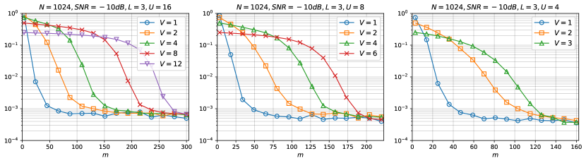
Figure 1: Average MSE_i for the active users dependent on the number of measurements $m$ for $n=1024$, SNR$=-10$dB, and $L=3$. The user number from left to right is $U=\{16,8,4\}$.

Our first simulation in Fig. 1 shows the dependence on $m$ where we depict the unnormalized frequency domain MSE_i per subcarrier for the active users averaged over the runs, see eq. (8). We see that the ’phase transitions’ occur for $m$ far less than $n$ as expected. From this simulation we obtain that $m=300$ is sufficient for the targeted parameter regime.

In Fig. 2 to Fig. 7 we simulated the user detection performance. Obviously, simulations and upper bounds coincide quite nicely and that in all cases the slope, i.e. diversity gain, is correctly represented justifying our approach for the analysis. Generally, the bounds qualitatively reflect the dependence on the system parameter in all cases provided $m$ is selected sufficiently large such that HiIHT operates far beyond the phase transition. This is clearly visible in Fig.’s 6, 7 where the performance is already worse for larger delay spread and even turns into an error floor for $k_{u}=12$ in Fig. 7. There is a small gap due to the union bound approach and the parameter $\epsilon$ which we never make explicit. Hence, generally, the parameter setting has to be carefully selected for the theorems to hold.

The user capacity gain is clearly visible in the simulation and is more than 300% since $m/n\leq 1/3$ which is a promising result. We have not incorporated the block correlator since it will operate in the order of our upper bounds as shown in [19]. This implies that we have not come close to the asymptotic regime where the hierarchical thresholding algorithm outperforms the block correlation detector.

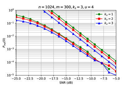
Figure 2: The Figure depicts $P_{\text{md}}$ over SNR for $n=1024,m=300,k_{s}=3,u=4.$

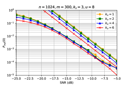
Figure 3: The Figure depicts $P_{\text{md}}$ over SNR for $n=1024,m=300,k_{s}=3,u=8.$

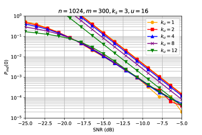
Figure 4: The Figure depicts $P_{\text{md}}$ over SNR for $n=1024,m=300,k_{s}=3,u=16.$

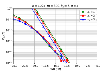
Figure 5: The Figure depicts $P_{\text{md}}$ over SNR for $n=1024,m=300,k_{s}=6,u=4.$

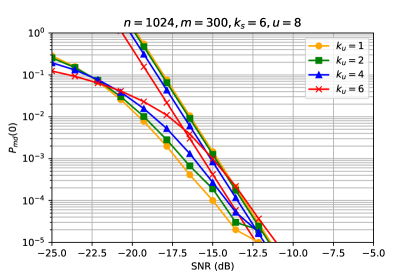
Figure 6: The Figure depicts $P_{\text{md}}$ over SNR for $n=1024,m=300,k_{s}=6,u=8.$

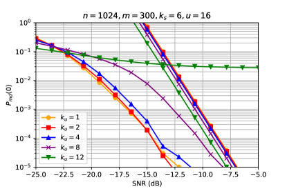
Figure 7: The Figure depicts $P_{\text{md}}$ over SNR for $n=1024,m=300,k_{s}=6,u=16.$

In Fig. 8 we evaluate finally the corresponding MSE performance. Also here we see that the performance of the detector is sufficient to obtain qualitatively good channel estimates in ’one shot’ random access scenarios.

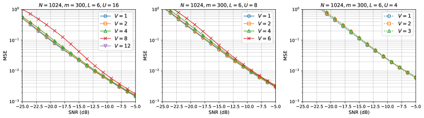
Figure 8: Average MSE_i dependent on the number of measurements $m$.

VI Conclusions and Outlook

In this paper, the performance of hierarchical thresholding algorithms under noise is studied for certain indicators, in particular, the block error and missed detection probability. We provide upper bounds on the missed detection probability in terms of the diversity order and relate them to the classical block correlation detector. Our findings are that in a certain sparse parameter regime the HiHTP detector can outperform the classical detection schemes. This parameter regime is expected to arise ubiquitously in mMTC scenarios.

Very recently, in a series of papers, mMTC system design is combined with massive MIMO which adds another design parameter (number of antennas) to the problem. In recent work [22], the Approximate Message Passing (AMP) algorithm is considered for the demanding setting where sparsity is growing linearly with the dimensions showing that detection probability can be driven to zero with large number of antennas. On the other hand frequency diversity is not considered in [22]. Another work can be found in [23] where approximative analysis is provided without considering multipath. Hence, it would be interesting to see the effect of multipath in our work in [18] where error rates tend to decrease with the same diversity order.

VII Acknowledgements

This work was carried out within DFG grants WU 598/7-1 and WU 598/8-1 (DFG Priority Program on Compressed Sensing). The research of IR and JE has been supported by the DFG project EI 519/9-1 (SPP1798 CoSIP), the Templeton Foundation, the EU (RAQUEL), the BMBF (Q.com), and the ERC (TAQ).

-A Proof of Theorem 2

We need the following proposition for any of the following theorems. The following proposition is the ’high SNR’ probability approximation of misdetection events which is used in Theorem 4 and Proposition 2.

Proposition 1.

Let $z_{0},\ldots,z_{u-1}\sim\mathcal{CN}\left(0,\sigma^{2}I_{m}\right)$ and $(h_{i})_{\mathcal{A}_{1}}\sim\mathcal{CN}\left(0,\operatorname{diag}\left(\sigma_{h,0}^{2},\sigma_{h,1}^{2},\ldots,\sigma_{h,k_{s}-1}^{2}\right)\right)$ with $\mathcal{A}\subset[s]$ some index set of size $|\mathcal{A}|=k_{s}<s$. Then

$$\mathbb{P}\left(\max\nolimits_{j\neq i}\|z_{j}\|^{2}\geq\|(h_{i})_{\mathcal{A}_{1}}\|^{2}\right)$$

$$=\frac{u\sigma^{2k_{s}}}{\prod_{i=0}^{k_{s}-1}\sigma_{h,i}^{2}}\sum_{j=0}^{m-1}\frac{\Gamma\left(k_{s}+j\right)}{\Gamma\left(k_{s}\right)j!}+o\left(\operatorname{SNR}^{k_{s}}\right).$$

Proof.

Fix $i=1$. Set $\|\left(h_{1}\right)_{\mathcal{A}}\|^{2}=:X$. Clearly, by the union bound

$$\mathbb{P}\left(\max\nolimits_{j>1}\|z_{j}\|^{2}>X\right)\leq\left(u-1\right)\mathbb{P}\left(\|z_{2}\|^{2}>X\right)$$

and conversely

$$\mathbb{P}\left(\max\nolimits_{j>1}\|z_{j}\|^{2}>X\right)$$

$$=1-\left(1-\mathbb{P}\left(\|z_{2}\|^{2}>X\right)\right)^{u-1}$$

$$=1-\exp\left(\left(u-1\right)\log\left(1-\mathbb{P}\left(\|z_{2}\|^{2}>X\right)\right)\right)$$

$$\geq 1-\exp\left(-\left(u-1\right)\mathbb{P}\left(\|z_{2}\|^{2}>X\right)\right)$$

$$\geq\left(u-1\right)\mathbb{P}\left(\|z_{2}\|^{2}>X\right)-{\textstyle\sum_{i=2}^{\infty}}\frac{u^{i}}{i!}\mathbb{P}^{i}\left(\|z_{2}\|^{2}>X\right)$$

$$\geq\left(u-1\right)\mathbb{P}\left(\|z_{2}\|^{2}>X\right)-\mathbb{P}^{2}\left(\|z_{2}\|^{2}>X\right){\textstyle\sum_{i=2}^{\infty}}\frac{u^{i}}{i!}$$

$$\geq\left(u-1\right)\mathbb{P}\left(\|z_{2}\|^{2}>X\right)-\mathbb{P}^{2}\left(\|z_{2}\|^{2}>X\right)e^{u}.$$

The first inequality follows from $\log\left(1-x\right)\leq-x$ and $\exp\left(x\right)$ is increasing over $\mathbb{R}$. The second inequality follows from expanding the exponential term. The third is due to $\mathbb{P}(\|z_{2}\|^{2}>X)<1$. Hence, for fixed $u$ we have the desired converse. To proceed, we denote the density of $X$ as $f_{X}$. We want to calculate

$$\mathbb{P}(\{\lVert z_{2}\rVert^{2}\geq X\})=\int\mathbb{P}(\lVert z_{2}\rVert^{2}\geq X|X=x)f_{X}(x)dx,.$$ (14)

The complementary cumulative distribution function for the squared norm of the complex Gaussian noise $z_{1}\sim\mathcal{CN}(0,\frac{\sigma^{2}}{n}I_{m})$ is given by [19]:

$$\mathbb{P}\left(\lVert z_{2}\rVert^{2}>x\right)=\sum_{j=0}^{m-1}\frac{x^{j}\exp\left(-\frac{x}{\sigma^{2}}\right)}{j!\sigma^{2j}}.$$ (15)

Moreover, it was shown in [24] and applied in [19], that the probability density function of $\gamma$ can be approximated around $\gamma=0$ in the high $\operatorname{SNR}$ regime by

$$f_{\gamma}\left(x\right)=\frac{\prod_{i=0}^{k_{s}-1}\sigma_{h,i}^{-2}}{\Gamma\left(k_{s}\right)}x^{k_{s}-1}+o\left(x^{k_{s}}\right).$$ (16)

Since the performance parameters depend only on the behaviour of the function near the origin, the part $o\left(x^{k_{s}}\right)$ can be neglected in the performance analysis for high $\operatorname{SNR}$ regimes. Plugging (16) and (15) into (14) yields:

$$\int\mathbb{P}(\lVert z_{2}\rVert^{2}\geq X\mid X=x)f_{X}(x)dx$$

$$=\frac{\prod_{i=0}^{k_{s}-1}\sigma_{h,i}^{-2}}{\Gamma\left(k_{s}\right)}\sum_{j=0}^{m-1}\frac{1}{j!\sigma^{2j}}\int\limits_{0}^{\infty}x^{k_{s}-1}x^{j}\exp\left(-\frac{x}{\sigma^{2}}\right)dx$$

$$=\frac{\prod_{i=0}^{k_{s}-1}\sigma_{h,i}^{-2}}{\Gamma\left(k_{s}\right)}\sum_{j=0}^{m-1}\frac{\Gamma\left(k_{s}+j\right)}{j!\sigma^{2j}}\left(\frac{1}{\sigma^{2}}\right)^{-k_{s}-j}$$

$$=\frac{\sigma^{2k_{s}}}{\prod_{i=0}^{k_{s}-1}\sigma_{i}^{2}}\sum_{j=0}^{m-1}\frac{\Gamma\left(k_{s}+j\right)}{\Gamma\left(k_{s}\right)j!}$$

where we used that

$$\int_{0}^{\infty}x^{k-1}e^{-Ax}dx=\Gamma\left(k\right)A^{-k}.$$ (17)

Observing that the result is independent of the actual support of $h_{i}$ completes the proof. ∎

We now provide a proof for the Theorem 2. For the proof it is sufficient to consider a single fixed user with index $i\in\mathcal{A}^{B}$ out of the atmost $k_{u}$ active users.

Proof of Theorem 2.

By the definition of the user detection scheme using HiHTP, the detection of a user requires two conditions to be met: First, the reconstructed block $h^{\ast}_{i}$ must be larger in $\ell_{2}$-norm than all blocks which were regarded as inactive. Second, the norm must exceed the energy threshold of $\sqrt{\xi}$. Thus, for the active $i$-th user to be missed at the same time at least one inactive user must be detected as active. In other words, the $\ell_{2}$-norm of the $i$-th block of $h^{\ast}$ is smaller than at least one block of $h^{\ast}$ with index in the complement $\overline{\mathcal{A}^{B}}$ of $\mathcal{A}^{B}$. Here, the complement is taken with respect to ${1,\ldots u}$. We therefore find that the event of “missed detection” of the $i$-th user is included as follows:

$$\left\{\text{missed detection of user }i\right\}$$

$$\subset\left\{\left\|h^{\ast}_{i}\right\|\leq\sqrt{\xi}\right\}\cup\left\{\max\nolimits_{j\in\overline{\mathcal{A}^{B}}}\left\|h^{\ast}_{j}\right\|\geq\left\|h^{\ast}_{i}\right\|\right\}.$$

Note that this inclusion is proper since the second event does not guarantee that the $i$-th user is not detected.

Let us abbreviate the difference between the recovered and the original signal by $d_{i}:=h^{\ast}_{i}-h_{i}$. The first event then implies the following conditions:

$$\left\{\left\|h^{\ast}_{i}\right\|\leq\sqrt{\xi}\right\}\equiv\left\{\left\|h^{\ast}_{i}-h_{i}+h_{i}\right\|\leq\sqrt{\xi}\right\}$$

$$\subseteq\left\{\left|\left\|d_{i}\right\|-\left\|h_{i}\right\|\right|\leq\sqrt{\xi}\right\}$$

$$\equiv\left\{-\sqrt{\xi}\leq\left\|d_{i}\right\|-\left\|h_{i}\right\|\leq\sqrt{\xi}\right\}$$

$$\subseteq\left\{\left\|h_{i}\right\|-\left\|d_{i}\right\|\leq\sqrt{\xi}\right\}\equiv\left\{\sqrt{\xi}+\left\|d_{i}\right\|\geq\left\|h_{i}\right\|\right\}$$

$$\subseteq\left\{\left\|d_{i}\right\|\geq\frac{1}{2}\left\|h_{i}\right\|\right\}\cup\left\{\sqrt{\xi}\geq\frac{1}{2}\left\|h_{i}\right\|\right\}$$

where $\mathbb{P}(\{\sqrt{\xi}\geq\frac{1}{2}\|h_{i}\|\})=F(4\xi)$. The second event requires that

$$\left\{\max\nolimits_{j\in\overline{\mathcal{A}^{B}}}\left\|h^{\ast}_{j}\right\|\geq\left\|h^{\ast}_{i}\right\|\right\}$$

$$\subseteq\left\{\max\nolimits_{j\in\overline{\mathcal{A}^{B}}}\left\|h^{\ast}_{j}-h_{j}\right\|\geq\left\|h^{\ast}_{i}-h_{i}+h_{i}\right\|\right\}$$

$$\subseteq\left\{\max\nolimits_{j\in[u]}\left\|d_{j}\right\|+\left\|d_{i}\right\|\geq\left\|h_{i}\right\|\right\}$$

$$\subseteq\left\{\left\|d\right\|\geq\frac{1}{2}\left\|h_{i}\right\|\right\}.$$

After squaring both sides, we can utilize Theorem 1 to show that

$$\mathbb{P}\left(\left\{4\left\|d\right\|^{2}\geq\left\|h_{i}\right\|^{2}\right\}\right)\leq\mathbb{P}_{\overline{\text{RIP}}}+\mathbb{P}\left(\left\{\frac{4\tau^{2}}{n}\lVert z\rVert^{2}\geq\left\|h_{i}\right\|^{2}\right\}\right).$$

Now we can invoke Prop. 1 to show that

$$\mathbb{P}\left(\left\{\frac{4\tau^{2}}{n}\lVert z\rVert^{2}\geq\left\|h_{i}\right\|^{2}\right\}\right)$$

$$\leq\left(\frac{4\tau^{2}\sigma^{2}}{n\sigma_{h}^{2}}\right)^{-k_{s}}B_{1}\left(m,k_{s}\right)$$

$$=\left(4\tau^{2}\right)^{k_{s}}n^{-k_{s}}\operatorname{SNR}^{-k_{s}}B_{1}(m,k_{s})$$

which concludes the proof. ∎

-B Proof of Lemma 1

The proof of Lemma 1 relies on concentration inequalities for the measurement map $A$ as well as the norm of the signal $h$ and the noise $z^{\prime}$ introduced as model (4).

Let us first introduce the norm concentration for a Gaussian linear mappings. Let $G\in\mathbb{C}^{m\times n}$ be a random matrix with i.i.d. Gaussian entries $\left(G\right)_{ki}\sim\mathcal{CN}(0,\frac{1}{m})$. The normalisation ensures that $\mathbb{E}\left\|Ax\right\|^{2}=\left\|x\right\|^{2}$ for any vector $x\in\mathbb{C}^{n}$. For a Gaussian random matrix, it holds that [25, Lemma 9.8]:

$$\mathbb{P}\left(\left|\left\|Ax\right\|^{2}-\left\|x\right\|^{2}\right|>\epsilon\left\|x\right\|^{2}\right)\leq 2e^{-\frac{\epsilon^{2}m}{2}}$$ (18)

for every $\epsilon\in(0,1)$.

This concentration inequality allows us to also derive a concentration bound for the the norm of a Gaussian random vector. To this end, we choose $m=n$ and the vector $x_{\sigma}\coloneqq(\sigma,\sigma,\ldots,\sigma)^{T}\in\mathbb{C}^{m}$. With this choice, we have that $x\coloneqq Ax_{\sigma}\sim\mathcal{CN}(0,\sigma^{2}I_{m})$ is a random vector with i.i.d. Gaussian entries of variance $\sigma^{2}$. From eq. (18) we conclude that

$$2e^{-\frac{\epsilon^{2}m}{2}} \geq\mathbb{P}\left(\left|\left\|Ax_{\sigma}\right\|^{2}-\left\|x_{\sigma}\right\|^{2}\right|>\epsilon\left\|x_{\sigma}\right\|^{2}\right)$$ (19)

$$\geq\mathbb{P}\left(\left\|x\right\|^{2}>\left(\epsilon+1\right)m\sigma^{2}\right)$$

$$+\mathbb{P}\left(\left\|x\right\|^{2}>\left(1-\epsilon\right)m\sigma^{2}\right)$$

and, thus,

$$\mathbb{P}\left(\left\|x\right\|^{2}>\epsilon\right)\leq 2e^{-\left(\frac{\epsilon}{m\sigma^{2}}-1\right)^{2}\frac{m}{2}.}$$ (20)

provided that $\epsilon/m\sigma^{2}>1$.

We will also need a concentration inequality for the measurement map $A$, that was argued to be a uniformly at random subsampled Fourier matrix. Unfortunately, random Fourier matrices to not directly fulfil a concentration inequality like (18) but only if we restrict $x$ to be sparse. Suppose $|\operatorname{supp}\left(x\right)|\leq k_{s}k_{u}$, then [25, Lemma 12.25] shows

$$\mathbb{P}\left(\left|\left\|Ax\right\|^{2}-\left\|x\right\|^{2}\right|>\left(\sqrt{\frac{k_{s}k_{u}}{m}}+\epsilon\right)\left\|x\right\|^{2}\right)$$

$$\leq 2e^{-\frac{\epsilon^{2}m}{2k_{s}k_{u}}\frac{1}{1+2\sqrt{k_{s}k_{u}/m}+\epsilon/3}}$$

$$\leq 2e^{-\frac{\epsilon^{2}m}{2\left(1+\epsilon\right)k_{s}k_{u}}}$$ (21)

for $m\gg k_{s}k_{u}$.

The assertion of Lemma 1 should hold for noisy signals of the form of (4). The model assumes that the signal is of the form $h^{z}\coloneqq h+z^{\prime}\in\mathbb{C}^{n}$, where the support of $h$ is a hierarchically $\left(k_{u},k_{s}\right)$-sparse set $\mathcal{A}$ drawn uniformly at random. The values of the entries are randomly chosen such that $(h^{z})_{\mathcal{A}}\sim\mathcal{CN}(0,(\sigma_{h}^{2}+m\sigma^{2}/n^{2})I_{k_{u}k_{s}})$ and $(h^{z})_{\mathcal{A}^{C}}\sim\mathcal{CN}(0,m\sigma^{2}/n^{2}I_{n-k_{u}k_{s}})$.

It is important to note that in this model the signal $h^{z}$ is not sparse due to the noise contribution. The following proposition will extend the concentration inequality for subsampled Fourier measurements to this signal model.

Proposition 2.

Let $A\in\mathbb{C}^{m\times n}$ be a randomly subsampled FFT and let $h,z^{\prime}$ obey the random model above. Then, it holds:

$$\mathbb{E}_{h}\mathbb{P}\left(\left|\left\|A\left(h+z^{\prime}\right)\right\|^{2}-\left\|h+z^{\prime}\right\|^{2}\right|>\epsilon\left\|h+z^{\prime}\right\|^{2}|h\right)$$

$$\leq 4e^{-\frac{\left(\epsilon-3t\right)^{2}m}{2\left(1+\epsilon-3t\right)k_{s}k_{u}}}+\frac{6\Gamma\left(k_{u}k_{s}/2\right)}{\Gamma\left(k_{u}k_{s}\right)}\left(\frac{t^{2}\operatorname{SNR}n}{2\left(1+\epsilon\right)}\right)^{-k_{s}k_{u}}$$

for sufficiently large SNR.

Proof.

In the proof we make use of the notation introduced as model (4). To this end, recall that $z=Az^{\prime}\in\mathbb{C}^{m}$ with $z\sim\mathcal{CN}\left(0,\frac{\sigma^{2}}{n}I_{m}\right),z^{\prime}\sim\mathcal{CN}\left(0,\frac{\sigma^{2}m}{n^{2}}I_{n}\right)$, and, hence, $\mathbb{E}\left\|z\right\|^{2}=\mathbb{E}\left\|z^{\prime}\right\|^{2}$. For the ease of notation, we set $\sigma_{m,n}^{2}\coloneqq\sigma^{2}m/n^{2}$ and $\sigma_{n}^{2}\coloneqq\sigma^{2}/n$. It holds that $\sigma_{n}^{2}m=\sigma_{m,n}^{2}n$.

Expanding $\left\|A\left(h+z^{\prime}\right)\right\|^{2}-\left\|h+z^{\prime}\right\|^{2}$ and adding zero yields

$$\left\|A\left(h+z^{\prime}\right)\right\|^{2}-\left\|h+z^{\prime}\right\|^{2}$$

$$=\left\|Ah\right\|^{2}+\left\|z\right\|^{2}-\mathbb{E}\left\|z\right\|^{2}+2\operatorname{Re}\left\langle\left(Ah\right),z\right\rangle$$

$$\quad\quad-\left\|h\right\|^{2}-\left\|z^{\prime}\right\|^{2}+\mathbb{E}\left\|z^{\prime}\right\|^{2}-2\operatorname{Re}\left\langle h,z^{\prime}\right\rangle.$$

Using the concentration of the norm of $z$ and $z^{\prime}$ as well as the measurement map, we can bound the individual terms of this expansion. Thus, for the first step we consider a constant $h$ and only view $z$, $z^{\prime}$ and $A$ as random variables. Let $s,t,o>0$ be small but fixed. Consider the event $\mathcal{C}_{1}$ defined by:

$$\left\{2\left|\operatorname{Re}\left\langle h,z^{\prime}\right\rangle\right|\leq s\sigma_{m,n}\left\|h\right\|\right\}$$

which, since $2\operatorname{Re}\left\langle\left(h\right),z^{\prime}\right\rangle$ is Gaussian, occurs with probability (at least ) $1-e^{-\frac{s^{2}}{2}}$ [25, Proposition 7.5, eq. (7.8)]. Similarly, the event $\mathcal{C}_{2}$ defined by:

$$\left\{2\left|\operatorname{Re}\left\langle Ah,z\right\rangle\right|\leq s\sigma_{n}\left\|Ah\right\|\right\}$$ (22)

$$\subseteq\left\{2\left|\operatorname{Re}\left\langle Ah,z\right\rangle\right|\leq s\sigma_{n}\left(1+2\epsilon\right)\left\|h\right\|\right\}$$

occurs at least with probability $1-e^{-\frac{s^{2}}{2}}+2e^{-\frac{\epsilon^{2}m}{2\left(1+\epsilon\right)k_{s}k_{u}}}$ for sufficiently large $m$ by eq. (21). Moreover, the events $\mathcal{C}_{3}$:

$$\left|\left\|z\right\|^{2}-\mathbb{E}\left\|z\right\|^{2}\right|\leq t\sigma_{n}^{2}m,$$

and $\mathcal{C}_{4}$:

$$\left|\left\|z^{\prime}\right\|^{2}-\mathbb{E}\left\|z^{\prime}\right\|^{2}\right|\leq t\sigma_{m,n}^{2}n$$

each occur with probabilities $1-2e^{-\frac{t^{2}m}{2}}$ and $1-2e^{-\frac{t^{2}n}{2}}$ by eq. (19), respectively. Eventually the event $\mathcal{C}_{5}$:

$$\left\|z^{\prime}\right\|^{2}<\left(1+o\right)n\sigma_{m,n}^{2}$$

occurs with probabilty of at least $1-2e^{-\frac{o^{2}n}{2}}$ by (20). Collect the joint event in ${\textstyle\bigcap_{i}}\mathcal{C}_{i}$. Define $\Lambda\left(h\right)\coloneqq|\left\|Ah\right\|^{2}-\left\|h\right\|^{2}|$. Conditioning on $h$, we get with $s_{\epsilon}\coloneqq s\left(1+2\epsilon\right)$ and $o_{1}\coloneqq 1+o$

$$\mathbb{P}\left(\left\{\left|\left\|A\left(h+z^{\prime}\right)\right\|^{2}-\left\|h+z^{\prime}\right\|^{2}\right|>\epsilon\left\|h+z^{\prime}\right\|^{2}\right\}\cap\mathcal{C}{\textstyle\bigcap_{i}}|h\right)$$

$$\leq\mathbb{P}\left(\left\{\Lambda\left(h\right)>\epsilon\left\|h+z^{\prime}\right\|^{2}-2s_{\epsilon}\sigma_{n}\left\|h\right\|-2t\sigma_{n}^{2}m\right\}\cap\mathcal{C}{\textstyle\bigcap_{i}}|h\right)$$

$$\leq\mathbb{P}\left(\left\{\Lambda\left(h\right)>\epsilon\left\|h\right\|^{2}-\left\|z^{\prime}\right\|^{2}-2s_{\epsilon}\sigma_{n}\left\|h\right\|-2t\sigma_{n}^{2}m\right\}\cap\mathcal{C}{\textstyle\bigcap_{i}}|h\right)$$

$$\leq\mathbb{P}\left(\left\{\frac{\Lambda\left(h\right)}{\left\|h\right\|^{2}}>\epsilon-\frac{2s_{\epsilon}\sigma_{n}}{\left\|h\right\|}-\frac{2t\sigma_{n}^{2}m}{\left\|h\right\|^{2}}-\frac{o_{1}n\sigma_{m,n}^{2}}{\left\|h\right\|^{2}}\right\}\cap\mathcal{C}{\textstyle\bigcap_{i}}|h\right).$$

Hence, we arrive at:

$$\mathbb{P}\left(\left|\left\|A\left(h+z^{\prime}\right)\right\|^{2}-\left\|h+z^{\prime}\right\|^{2}\right|>\epsilon\left\|h+z^{\prime}\right\|^{2}|h\right)$$

$$\leq 4e^{-\frac{\left(\epsilon-s^{\prime}+t^{\prime}+o^{\prime}\right)^{2}m}{2\left(1+\epsilon-s^{\prime}+t^{\prime}+o^{\prime}\right)k_{s}k_{u}}}$$ (23)

$$+2e^{-\frac{s^{\prime 2}\left\|h\right\|^{2}}{2\left(1+2\epsilon\right)^{2}\sigma_{n}^{2}}}+2e^{-\left(\frac{t^{\prime}\left\|h\right\|^{2}}{2m\sigma_{n}^{2}}\right)^{2}\frac{m}{2}}+2e^{-\left(\frac{o^{\prime}\left\|h\right\|^{2}}{n\sigma_{m,n}^{2}}-1\right)^{2}\frac{n}{2}}$$ (24)

where the term in eq. (23) is again due to (21) and $s^{\prime}:=\frac{2s_{\epsilon}\sigma_{n}}{\left\|h\right\|},t^{\prime}:=\frac{2t\sigma_{n}^{2}m}{\left\|h\right\|^{2}},o^{\prime}:=\frac{o_{1}n\sigma_{m,n}^{2}}{\left\|h\right\|^{2}}$ are the respective substitute variables. Note that we ‘shuffled’ the $\epsilon$-dependent exponential term from eq. (22) above into this first term as well. The terms in eq. (24) are due to bounding the probabilities of events $\mathcal{C}_{1}^{C}-\mathcal{C}_{5}^{C}$.

We shall now calculate the expectation value with respect to $h$. Since the expressions are exponentially decaying, it suffices to consider small $\left\|h\right\|^{2}$ with corresponding approximate pdf of eq. (16). This yields for the $s^{\prime}$-dependent term:

$$\frac{1}{\Gamma\left(k_{u}k_{s}\right)}\int_{0}^{\infty}e^{-\frac{s^{\prime 2}x}{2\left(1+\epsilon\right)\sigma_{n}^{2}}}x^{k_{s}k_{u}-1}dx$$

$$=\left(\frac{s^{\prime 2}\operatorname{SNR}n}{2\left(1+\epsilon\right)}\right)^{-k_{s}k_{u}}$$

using eq. (17). For the $t^{\prime}$-dependent and the $o^{\prime}$-dependent terms we get for some (even) $k_{u}$:

$$\frac{1}{\Gamma\left(k_{u}k_{s}\right)}\int_{0}^{\infty}e^{-\frac{t^{\prime 2}x^{2}}{2m\sigma_{n}^{4}}}x^{k_{s}k_{u}-1}dx$$

$$=\frac{1}{2\Gamma\left(k_{u}k_{s}\right)}\int_{0}^{\infty}e^{-\frac{t^{\prime 2}u}{2m\sigma_{n}^{4}}}u^{k_{s}k_{u}/2-1}du$$

$$=\frac{\Gamma\left(k_{u}k_{s}/2\right)}{2\Gamma\left(k_{u}k_{s}\right)}\left(\frac{t^{\prime 2}\operatorname{SNR}^{2}n^{4}}{2m^{3}}\right)^{-k_{s}k_{u}/2}.$$

The latter expression decays much faster than the first integral in the limit of $n\gg m\gg k_{s}k_{u}$. Altogether, we get for any small $\epsilon,t,\epsilon>3t$:

$$\mathbb{P}\left(\left|\left\|A\left(h+z^{\prime}\right)\right\|^{2}-\left\|h+z^{\prime}\right\|^{2}\right|>\epsilon\left\|h+z^{\prime}\right\|^{2}|h\right)$$

$$\leq 4e^{-\frac{\left(\epsilon-3t\right)^{2}m}{2\left(1+\epsilon-3t\right)k_{s}k_{u}}}+\frac{6\Gamma\left(k_{u}k_{s}/2\right)}{\Gamma\left(k_{u}k_{s}\right)}\left(\frac{t^{2}\operatorname{SNR}n}{2\left(1+\epsilon\right)}\right)^{-k_{s}k_{u}}$$ (25)

which holds for sufficiently large SNR. ∎

We turn back again to the proof of the lemma. We prove the result by using a linear estimator of the form $\Psi:=A^{H}$ which is essentially the first step of HiHTP and a subsequent energy detection per block.

Proof of Lemma 1.

Let $h^{z}=h+z^{\prime}$. We defined $\mathbb{P}_{\overline{\text{sRIP}}}$ as the probability of events of the form:

$$\left|\sum_{j\in\omega}\left|\left\langle h^{z},v_{j}\right\rangle\right|^{2}-\sum_{j\in\omega}\left|\left\langle\Psi y,v_{j}\right\rangle\right|^{2}\right|>\epsilon,$$

where $\omega\in\Omega_{i}$ for some $i\in[u]$ is some support set of cardinality $k_{s}$. Straightforward calculation gives

$$\left|\sum_{j\in\omega}\left(\left|\left\langle h^{z},v_{j}\right\rangle\right|^{2}-\left|\left\langle\Psi y,v_{j}\right\rangle\right|^{2}\right)\right|$$

$$=\left|\sum_{j\in\omega}\left(\left|\left\langle h^{z},v_{j}\right\rangle\right|+\left|\left\langle\Psi y,v_{j}\right\rangle\right|\right)\left(\left|\left\langle h^{z},v_{j}\right\rangle\right|-\left|\left\langle\Psi y,v_{j}\right\rangle\right|\right)\right|$$

$$\leq\max_{j\in\omega}\left|\left|\left\langle h^{z},v_{j}\right\rangle\right|-\left|\left\langle\Psi y,v_{j}\right\rangle\right|\right|(\sum_{j\in\omega}\left|\left\langle h^{z},v_{j}\right\rangle\right|+\sum_{j\in\omega}\left|\left\langle\Psi y,v_{j}\right\rangle\right|)$$

For the linear estimator under consideration $\Psi=A^{H}$, it holds that $\left\langle\Psi y,v_{j}\right\rangle=\left\langle A^{H}Ah^{z},v_{j}\right\rangle=\left\langle Ah^{z},Av_{j}\right\rangle$. The second term can hence be bounded by

$$\sum_{j\in\omega}\left|\left\langle h^{z},v_{j}\right\rangle\right|+\sum_{j\in\omega}\left|\left\langle\Psi y,v_{j}\right\rangle\right|$$

$$\leq\sqrt{|\omega|}(\sum_{j\in\omega}\left|h_{j}^{z}\right|^{2})^{1/2}+\sum_{j\in\omega}\left|\left\langle Ah^{z},Av_{j}\right\rangle\right|$$

$$\leq\sqrt{|\omega|}(\sum_{j\in\omega}\left|h_{j}^{z}\right|^{2})^{1/2}+\left\|Ah^{z}\right\|\sum_{j\in\omega}\left\|Av_{j}\right\|$$

$$\leq\sqrt{|\omega|}(\sum_{j\in\omega}\left|h_{j}^{z}\right|^{2})^{1/2}+\left(1+2\epsilon\right)\left\|h^{z}\right\|\sqrt{|\omega|}$$

$$\leq 2\left(1+2\epsilon\right)\sqrt{k_{s}}\left\|h^{z}\right\|.$$

with probability:

$$1-2e^{-\frac{\epsilon^{2}m}{2\left(1+\epsilon\right)k_{s}k_{u}}}$$ (26)

The complementary event can again be shuffled into the term in eq. (23).

Now, we turn to bound the first term. By using the reverse triangle inequality and the polarization identity:

$$\left\langle h^{z},v_{j}\right\rangle=\frac{1}{4}\sum_{k=0}^{3}\imath^{k}\left\|h^{z}+\imath^{k}v_{j}\right\|^{2},$$

we get:

$$\max_{j\in\omega}\left|\left|\left\langle h^{z},v_{j}\right\rangle\right|-\left|\left\langle Ah^{z},Av_{j}\right\rangle\right|\right|$$

$$\leq\max_{j\in\omega}\left|\left\langle h^{z},v_{j}\right\rangle-\left\langle Ah^{z},Av_{j}\right\rangle\right|$$

$$\leq\frac{1}{4}\max_{j\in\omega}\left|\sum_{k=0}^{3}\imath^{k}\left(\left\|h^{z}+\imath^{k}v_{j}\right\|^{2}-\left\|A\left(h^{z}+\imath^{k}v_{j}\right)\right\|^{2}\right)\right|$$

$$\leq\max_{j\in\omega,k\in[4]}\left|\left(\left\|h^{z}+\imath^{k}v_{j}\right\|^{2}-\left\|A\left(h^{z}+\imath^{k}v_{j}\right)\right\|^{2}\right)\right|.$$

We define $\xi_{j}^{k}\coloneqq h^{z}+\imath^{k}v_{j}$ and abbreviate the summation $\sum_{i,\omega,j,k}\coloneqq\sum_{i\in[u]}\sum_{\omega\in\Omega_{i}}\sum_{j\in\omega}\sum_{k\in[4]}$. Collecting all the terms and ‘averaging’ over $h$ yields

$$\mathbb{E}_{h}\Pr\left(\max_{i\in[u],\omega\in\Omega_{i}}\left|\sum_{j\in\omega}\left(\left|\left\langle h^{z},v_{j}\right\rangle\right|^{2}-\left|\left\langle\Psi y,v_{j}\right\rangle\right|^{2}\right)\right|>\epsilon|h\right)$$

$$\leq\sum_{i,\omega,j,k}\mathbb{E}_{h}\Pr\left(\left|\left\|\xi_{j}^{k}\right\|^{2}-\left\|A\xi_{j}^{k}\right\|^{2}\right|>\frac{\epsilon}{2\sqrt{k_{s}}\left\|h^{z}\right\|}|h\right)$$

$$=\sum_{i,\omega,j,k}\mathbb{E}_{h}\Pr\left(\left|\left\|\xi_{j}^{k}\right\|^{2}-\left\|A\xi_{j}^{k}\right\|^{2}\right|>\frac{\epsilon\left\|\xi_{j}^{k}\right\|^{2}}{2\sqrt{k_{s}}\left\|h^{z}\right\|\left\|\xi_{j}^{k}\right\|^{2}}|h\right),$$

where we used the union bound. For appropriately small constants $s,o>0$, we have

$$2\sqrt{k_{s}}\left\|h^{z}\right\|\left\|\xi_{j}^{k}\right\|^{2}$$

$$=O\left(2\sqrt{k_{s}}\left\|h\right\|^{3}\left(2+\sqrt{\left(s+1\right)n}\sigma_{m,n}\right)^{3}\right)$$

$$=O\left(2\sqrt{k_{s}}\left\|h\right\|^{3}\left(2+\sqrt{\left(s+1\right)\frac{m}{n}}\sigma\right)^{3}\right)$$

with probability of at least $1-2e^{-\frac{s^{2}n}{2}}$ by eq. (20) and provided $\left\|h\right\|^{2}\geq 1$; moreover, $\left(1-o\right)k_{u}k_{s}\leq\left\|h\right\|^{2}\leq\left(1+o\right)k_{u}k_{s}$ with probability $1-2e^{-\frac{o^{2}k_{u}k_{s}}{2}}$ by eq. (19). Hence, altogether, we arrive at

$$2\sqrt{k_{s}}\left\|h^{z}\right\|\left\|\xi_{j}^{k}\right\|^{2}$$

$$=O\left(2\sqrt{k_{s}}\left(\left(1+o\right)k_{u}k_{s}\right)^{\frac{3}{2}}\left(2+\sqrt{\left(s+1\right)\frac{m}{n}}\sigma\right)^{3}\right)$$

$$=O\left(k_{u}^{3/2}k_{s}^{2}\left(1+o\right)^{3/2}\left(1+s\right)^{3/2}\right).$$

with probability $1-2e^{-\frac{s^{2}n}{2}}-2e^{-\frac{o^{2}k_{u}k_{s}}{2}}$.

Except for the noise floor $z^{\prime}$ in $h^{z}$, the vectors $\xi_{j}^{k}=h^{z}+\imath^{k}v_{j}$ are $\left(k_{u}k_{s}+1\right)$-sparse. Fix some small $\epsilon>0,o=s=1$, and let $\epsilon^{\prime}\in O(\epsilon k_{u}^{-3/2}k_{s}^{-2})$. We can invoke Prop. 2 to give:

$$\sum_{i,\omega,j,k}\mathbb{E}_{h}\Pr\left(\left|\left\|\xi_{j}^{k}\right\|^{2}-\left\|A\xi_{j}^{k}\right\|^{2}\right|>\epsilon^{\prime}\left\|\xi_{j}^{k}\right\|^{2}|h\right)$$

$$\leq 32u\binom{s}{k_{s}}k_{s}\left[6e^{-\frac{\left(\epsilon^{\prime}-3t\right)^{2}m}{2\left(1+\epsilon^{\prime}-3t\right)\left(k_{u}k_{s}+1\right)}}\right.$$

$$\left.+\frac{6\Gamma\left(k_{u}k_{s}/2\right)}{\Gamma\left(k_{u}k_{s}\right)}\left(\frac{t^{2}\operatorname{SNR}n}{2\left(1+\epsilon^{\prime}\right)}\right)^{-k_{u}k_{s}}\right]+4e^{-\frac{k_{u}k_{s}}{2}}$$

for sufficiently large SNR.

Here, we included the term in (26) into the first exponential term in the second line. Assume $1\leq\left(1+\epsilon^{\prime}\right),\left(1+\epsilon^{\prime}-3t\right)<2$ with $\epsilon^{\prime}>3t$. Setting $t=k_{u}^{-2}k_{s}^{-2.5}$ yields $3t(\epsilon^{\prime})^{-1}=3t\epsilon^{-1}k_{u}^{3/2}k_{s}^{2}\rightarrow 0$ as required and hence:

$$\sum_{i,\omega,j,k}\mathbb{E}_{h}\Pr\left(\left|\left\|\xi_{j}^{k}\right\|^{2}-\left\|A\xi_{j}^{k}\right\|^{2}\right|>\epsilon^{\prime}\left\|\xi_{j}^{k}\right\|^{2}|h\right)$$

$$\leq 32u\binom{s}{k_{s}}k_{s}e^{-\frac{\epsilon^{\prime 2}\left(1-3t/\epsilon^{\prime}\right)^{2}m}{4k_{u}k_{s}}}$$

$$+\frac{32u\binom{s}{k_{s}}k_{s}\Gamma\left(k_{u}k_{s}/2\right)}{\Gamma\left(k_{u}k_{s}\right)}\left(\frac{t^{2}\operatorname{SNR}n}{4}\right)^{-k_{u}k_{s}}+4e^{\frac{-k_{u}k_{s}}{2}}$$

$$\leq 32u\binom{s}{k_{s}}k_{s}e^{-\frac{\epsilon^{2}m}{O\left(4k_{u}^{4}k_{s}^{5}\right)}}$$

$$+\frac{32u\binom{s}{k_{s}}k_{s}\Gamma\left(k_{u}k_{s}/2\right)}{\Gamma\left(k_{u}k_{s}\right)}\left(\frac{\operatorname{SNR}n}{4k_{u}^{4}k_{s}^{5}}\right)^{-k_{u}k_{s}}+4e^{\frac{-k_{u}k_{s}}{2}}$$

for sufficiently large $k_{u}k_{s}$ (and SNR). By the standard inequality $\binom{s}{k_{s}}\leq\left(\frac{es}{k_{s}}\right)^{k_{s}}$ for the binominal coefficient, the first term in the last line can be bounded as:

$$32u\binom{s}{k_{s}}k_{s}e^{-\frac{\epsilon^{2}m}{O\left(4k_{u}^{4}k_{s}^{5}\right)}}\leq 32u\left(\frac{es}{k_{s}}\right)^{k_{s}}k_{s}e^{-\frac{\epsilon^{2}m}{O\left(4k_{u}^{4}k_{s}^{5}\right)}}$$

while by Stirling’s approximation for the gamma functions $\Gamma(n)=(n-1)!$ for some positive integer $n>0$, we have for the second term:

$$\frac{32u\binom{s}{k_{s}}k_{s}\Gamma\left(k_{u}k_{s}/2\right)}{\Gamma\left(k_{u}k_{s}\right)}\left(\frac{\operatorname{SNR}n}{4k_{u}^{4}k_{s}^{5}}\right)^{-k_{u}k_{s}}$$

$$\leq\frac{32}{\sqrt{2}}\operatorname{SNR}^{-k_{u}k_{s}}n^{-2k_{s}}u\left(\frac{es}{k_{s}}\right)^{k_{s}}k_{s}$$

$$\cdot\left(\frac{e}{2}\right)^{k_{u}k_{s}/2}\left(k_{u}k_{s}\right)^{-k_{u}k_{s}/2}n^{-k_{u}k_{s}}n^{2k_{s}}\left(4k_{u}^{4}k_{s}^{5}\right)^{k_{u}k_{s}}$$

$$\leq\frac{32k_{s}}{\sqrt{2}}\operatorname{SNR}^{-k_{u}k_{s}}n^{-2k_{s}}\left(\frac{e}{k_{s}}\right)^{k_{s}}$$

$$\cdot\left(\frac{8e}{k_{u}k_{s}}\right)^{k_{u}k_{s}/2}\left(\frac{k_{u}^{4}k_{s}^{5}}{n^{(1-3/k_{u})}}\right)^{k_{u}k_{s}}$$

$$\leq\frac{32k_{s}}{\sqrt{2}}\frac{\operatorname{SNR}^{-k_{u}k_{s}}}{n^{2k_{s}}}\left(\frac{k_{u}^{4}k_{s}^{5}}{n^{(1-3/k_{u})}}\right)^{k_{u}k_{s}}$$

where the last term holds for $k_{u}\geq 8,k_{s}\geq 3$ which gives the final result. ∎

-C Proof of Theorem 4

The idea of the proof is to estimate $h^{z}=h+z^{\prime}$ directly instead of $h$. Thus, we consider some $h^{z}$ be fixed. For simplicity, let $h^{\ast}$ be again the estimator for $h^{z}$. Suppose user $i$ is active (and at most $k_{u}-1$ arbitrary other users). Denote again the true support of $h$ by $\mathcal{A}$. As discussed before, the estimation is equivalent:

$$y_{\mathcal{B}}=A\left(h+z^{\prime}\right)$$

where $z^{\prime}\sim\mathcal{CN}\left(0,\varkappa^{2}I_{m}\right)$ where $\varkappa^{2}=\frac{\sigma^{2}m}{nus}$.

Analogously, to the beginning of the proof of Theorem 2, we have

$$\left\{\text{missed detection of user }i\right\}$$

$$\subset\left\{\|(h^{\ast}_{i})_{\omega(h^{\ast}_{i})}\|\leq\sqrt{\xi}\right\}\cup\left\{\max_{j\in\overline{\mathcal{A}^{B}}}\|(h^{\ast}_{j})_{\omega(h^{\ast}_{j})}\|\geq\|(h^{\ast}_{i})_{\omega(h^{\ast}_{i})}\|\right\}$$

where $\omega(h^{\ast}_{i})$, $\omega(h^{\ast}_{j})$ are the support sets of the $k_{s}$ largest elements of $|h^{\ast}_{i}|$, $|h^{\ast}_{j}|$, respectively. By Lemma 1, HiHTP/HiIHT recovers $\|(h_{i}^{z})_{\omega}\|^{2}$ within $\epsilon$-vicinity with probability $\mathbb{P}_{\overline{\text{sRIP}}}\left(\epsilon\right)$ uniformly for all $i$ and all support sets $\omega$. Hence, we have for the first event:

$$\left\{\|(h^{\ast}_{i})_{\omega(h^{\ast}_{i})}\|^{2}\leq\xi\right\}$$

$$\subseteq\left\{\|(h^{\ast}_{i})_{\mathcal{A}_{i}}\|^{2}\leq\xi\right\}$$

$$\subseteq\left\{\|(h_{i}+z_{i}^{\prime})_{\mathcal{A}_{i}}\|^{2}\leq\xi+\epsilon\right\}.$$

Moreover, for the second event:

$$\left\{\max\nolimits_{j\in\overline{\mathcal{A}^{B}}}\|(h^{\ast}_{j})_{\omega(h^{\ast}_{j})}\|^{2}\geq\|(h^{\ast}_{i})_{\omega(h^{\ast}_{i})}\|\right\}$$

$$\subseteq\left\{\max\nolimits_{j\in\overline{\mathcal{A}^{B}}}\|(z_{j}^{\prime})_{\omega(z_{j}^{\prime})}\|^{2}+\epsilon\geq\|(h_{i}+z_{i}^{\prime})_{\mathcal{A}_{i}}\|^{2}-\epsilon\right\}$$

$$\subseteq{\textstyle\bigcup\limits_{j\in\overline{\mathcal{A}^{B}}}}\left\{\|(z_{j}^{\prime})_{\omega(z_{j}^{\prime})}\|^{2}+\epsilon\geq\|(h_{i}+z_{i}^{\prime})_{\mathcal{A}_{i}}\|^{2}-\epsilon\right\}$$

$$\subseteq{\textstyle\bigcup\limits_{j\in\overline{\mathcal{A}^{B}}}}\left\{k_{s}\max_{k}|(z_{j}^{\prime})_{k}|^{2}+\epsilon\geq\|(h_{i}+z_{i}^{\prime})_{\mathcal{A}_{i}}\|^{2}-\epsilon\right\}$$

$$\subseteq{\textstyle\bigcup\limits_{j\in\overline{\mathcal{A}^{B}}}}{\textstyle\bigcup\limits_{k\in\mathcal{A}_{j}}}\left\{|\sqrt{k_{s}}(z_{j}^{\prime})_{k}|^{2}+\epsilon\geq\|(h_{i}+z_{i}^{\prime})_{\mathcal{A}_{i}}\|^{2}-\epsilon\right\}$$

$$\subseteq{\textstyle\bigcup\limits_{j\in\overline{\mathcal{A}^{B}}}}{\textstyle\bigcup\limits_{k\in\mathcal{A}_{j}}}\left\{\left\{|\sqrt{2k_{s}}(z_{j}^{\prime})_{k}|^{2}\geq\|(h_{i}+z_{i}^{\prime})_{\mathcal{A}_{i}}\|^{2}\right\}\right.$$

$$\left.\cup\left\{4\epsilon\geq\|(h_{i}+z_{i}^{\prime})_{\mathcal{A}_{i}}\|^{2}\right\}\right\}.$$

The first term in the last line can be bounded by $n^{-k_{s}}\left(\frac{us}{2k_{s}m}\right)^{-k_{s}}\operatorname{SNR}^{-k_{s}}s\left(u-k_{u}\right)B_{1}\left(1,k_{s}\right)$ with using the result for the block correlator and since the noise in $z_{i}^{\prime}$ is damped with $\left(\frac{2m}{us}\right)$. Now, averaging over all $h$ gives the result. ∎

References

• [1] G. Wunder, H. Boche, T. Strohmer, and P. Jung, “Sparse Signal Processing Concepts for Efficient 5G System Design,” IEEE ACCESS, December 2015. [Online]. Available: http://arxiv.org/abs/1411.0435
• [2] L. Applebaum, W. Bajwa, M. F. Duarte, and R. Calderbank, “Asynchronous Code-Division Random Access Using Convex Optimization,” Physical Communication, vol. 5, no. 2, pp. 129–147, February 2012.
• [3] H. Zhu and G. Giannakis, “Exploiting Sparse User Activity in Multiuser Detection,” IEEE Transactions on Communications, vol. 59, no. 2, pp. 454–465, 2011.
• [4] C. Bockelmann, H. F. Schepker, and A. Dekorsy, “Compressive sensing based multi-user detection for machine-to-machine communication,” Transactions on Emerging Telecommunications Technologies, vol. 24, no. 4, pp. 389–400, 2013. [Online]. Available: http://dx.doi.org/10.1002/ett.2633
• [5] Y. Ji, C. Stefanovic, C. Bockelmann, A. Dekorsy, and P. Popovski, “Characterization of Coded Random Access with Compressive Sensing based Multi-User Detection,” in Proc. of IEEE Globecom 2014, Austin, TX, USA, Dec. 2014. [Online]. Available: www.arxiv.com/1404.2119
• [6] J. Choi, “Two-stage multiple access for many devices of unique identifications over frequency-selective fading channels,” IEEE Internet of Things Journal, vol. 4, no. 1, pp. 162–171, Feb 2017.
• [7] ——, “Compressive random access with coded sparse identification vectors for mtc,” IEEE Transactions on Communications, vol. 66, no. 2, pp. 819–829, February 2017.
• [8] G. Wunder, P. Jung, and C. Wang, “Compressive Random Access for Post-LTE Systems,” in IEEE International Conf. on Commun. (ICC’14) – Workshop MASSAP, Sydney, Australia, May 2014.
• [9] G. Wunder, P. Jung, and M. Ramadan, “Compressive Random Access Using A Common Overloaded Control Channel,” in IEEE Global Communications Conference (Globecom’14) – Workshop on 5G & Beyond, San Diego, USA, December 2015. [Online]. Available: www.arxiv.com/1504.05318
• [10] G. Wunder, C. Stefanovic, and P. Popovski, “Compressive Coded Random Access for Massive MTC Traffic in 5G Systems,” in 49th Annual Asilomar Conf. on Signals, Systems, Pacific Grove, USA, November 2015, invited paper.
• [11] G. Wunder, I. Roth, R. Fritschek, and J. Eisert, “Hihtp: A custom-tailored hierarchical sparse detector for massive mtc,” in 2017 51st Asilomar Conference on Signals, Systems, and Computers, Oct 2017, pp. 1929–1934.
• [12] C. Bockermann, N. Patras, G. Wunder, and et al, “Towards Massive Connectivity Support for Scalable mMTC Communications in 5G networks,” IEEE ACCESS, May 2018. [Online]. Available: https://arxiv.org/abs/1804.01701
• [13] C. Bockelmann, N. Pratas, H. Nikopour, K. Au, T. Svensson, C. Stefanovic, P. Popovski, and A. Dekorsy, “Massive machine-type communications in 5g: physical and mac-layer solutions,” IEEE Communications Magazine, vol. 54, no. 9, pp. 59–65, September 2016.
• [14] F. Schaich et al, “FANTASTIC-5G: Flexible Air Interface for Scalable Service Delivery within Wireless Communication Networks of the 5th Generation,” Transactions on Emerging Telecommunications Technologies, vol. 27, no. 9, pp. 1216–1224, June 2016.
• [15] I. Roth, M. Kliesch, J. Eisert, and G. Wunder, “Reliable recovery of hierarchically sparse signals and application in machine-type communications,” arXiv preprint arXiv:1612.07806, 2016.
• [16] P. Sprechmann, I. Ramirez, G. Sapiro, and Y. C. Eldar, “C-HiLasso: A collaborative hierarchical sparse modeling framework,” IEEE Trans. Sig. Proc., vol. 59, pp. 4183–4198, 2011.
• [17] C. B. Henning F. Schepker and A. Dekorsy, “Exploiting Sparsity in Channel and Data Estimation for Sporadic Multi-User Communication,” in International Symposium on Wireless Communication Systems (ISWCS), Ilmenau, Germany, Aug. 2013.
• [18] G. Wunder, S. Stefanatos, A. Flinth, I. Roth, and G. Caire, “Low-overhead hierarchically-sparse channel estimation for multiuser wideband massive mimo,” ArXiv e-prints, June 2018. [Online]. Available: http://arxiv.org/abs/1806.00815
• [19] K. Lee, J. Kim, J. Jung, and I. Lee, “Zadoff-chu sequence based signature identification for ofdm,” IEEE Transactions on Wireless Communications, vol. 12, no. 10, pp. 4932–4942, October 2013.
• [20] J. Ling, D. Chizhik, A. Tulino, and I. Esnaola, “Compressed sensing algorithms for ofdm channel estimation,” ArXiv e-prints, December 2016. [Online]. Available: https://arxiv.org/abs/1612.07761
• [21] R. G. Baraniuk, V. Cevher, M. F. Duarte, and C. Hegde, “Model-based compressive sensing,” IEEE Trans. Inf. Th., vol. 56, no. 4, pp. 1982–2001, April 2010.
• [22] L. Liu and W. Yu, “Massive connectivity with massive mimo-part ii: User detection,” ArXiv e-prints, Januar 2017. [Online]. Available: https://arxiv.org/pdf/1706.06433.pdf
• [23] E. de Carvalho, E. Björnson, J. H. Sorensen, E. G. Larsson, and P. Popovski, “Random pilot and data access in massive mimo for machine-type communications,” IEEE Transactions on Wireless Communications, Januar 2017.
• [24] Z. Wang and G. B. Giannakis, “A simple and general parameterization quantifying performance in fading channels,” IEEE Transactions on Communications, vol. 51, no. 8, pp. 1389–1398, Aug 2003.
• [25] S. Foucart and H. Rauhut, A mathematical introduction to Compressed Sensing.   Birkhäuser, 2013.