A stratified age-period-cohort model for spatial heterogeneity in all-cause mortality

Abstract

A common goal in modeling demographic rates is to compare two or more groups. For example comparing mortality rates between men and women or between geographic regions may reveal health inequalities. A popular class of models for all-cause mortality as well as incidence of specific diseases like cancer is the age-period-cohort (APC) model. Extending this model to the multivariate setting is not straightforward because the univariate APC model suffers from well-known identifiability problems. Often APC models are fit separately for each strata, and then comparisons are made post hoc. This paper introduces a stratified APC model to directly assess the sources of heterogeneity in mortality rates using a Bayesian hierarchical model with matrix-normal priors that share information on linear and nonlinear aspects of the APC effects across strata. Computing, model selection, and prior specification are addressed and the model is then applied to all-cause mortality data from the European Union.

Keywords: Bayesian age-period-cohort analysis, spatio-temporal models, human mortality database, demographic statistics

1 Introduction and Running Example

Age-period-cohort (APC) models are used to model demographic rates including all-cause mortality as well as incidence of specific diseases like cancer. APC analysis is conceptually attractive because the models capture the major time scales along which disease rates evolve where direct measurements of the disease generating processes at the population scale are difficult or impossible to gather. Age effects are a surrogate for cumulative wear and tear on the body, period (time of event) effects for short acting exposures or new treatments, and cohort (time of birth) effects for longer acting exposures such as smoking. APC models are used to smooth out time trends in disease, forecast future numbers of cases, and give clues for the most important etiological factors. However they suffer from a well known identifiability issue wherein the linear trends along these time scales cannot be disentangled without adding additional constraints.

A common goal in applications of APC models is to compare disease rates across groups such as sexes, disease subtypes, or regions. Often this is done by post-hoc comparisons of separate APC models. In a recent example, Wang et al. (2018) fit separate models to drowning rates for males and females in China using the APC web-tool from the US National Institutes of Health (Rosenberg et al., 2014) and then compared graphically. The dominant approach when multivariate APC analyses are done is based on multivariate Gaussian Markov random fields (GMRFs) (Riebler and Held, 2010; Riebler et al., 2012a; Papoila et al., 2014). Typical implementations of univariate GMRFs include linear constraints, which then mask identifiability issues in multivariate extensions.

We resolve these issues with a novel stratified APC model based on non-linear aspects of the age, period, and cohort effects that are identifiable. We previously considered this parameterization in a Bayesian context for univariate APC models in (Smith and Wakefield, 2016). A Bayesian hierarchical model with matrix-normal priors allows for pooling of information on these identifiable terms across strata, and we carefully consider the specification of cross-correlation structures and prior distributions. Practical issues such as computing with r-INLA and model selection are also discussed.

We apply this model to mortality rates in 25 European Union (EU) countries from the Human Mortality Database (HMD). The HMD contains raw data on births and deaths reported by the national statistics offices of 39 countries as well as computed mortality rates and life tables. While not directly shareable, the data are free to download after registration (http://www.mortality.org). Figure 1 shows the single age-year death rates on the log scale for 25 EU countries. Cyprus, Malta and Romania are not covered by the HMD. Several interesting features of this data are immediately apparent. First, the mortality series are of very different lengths. While some countries in northern and western Europe (e.g., Denmark or France) have very long series dating back even before 1900, a common start year for data from countries in eastern Europe is 1959, the year of the first Soviet Census after World War II (Schwartz, 1986). Some of the shorter series (e.g., Croatia or Ireland) are related to countries becoming independent or in the case of Germany, reunified.

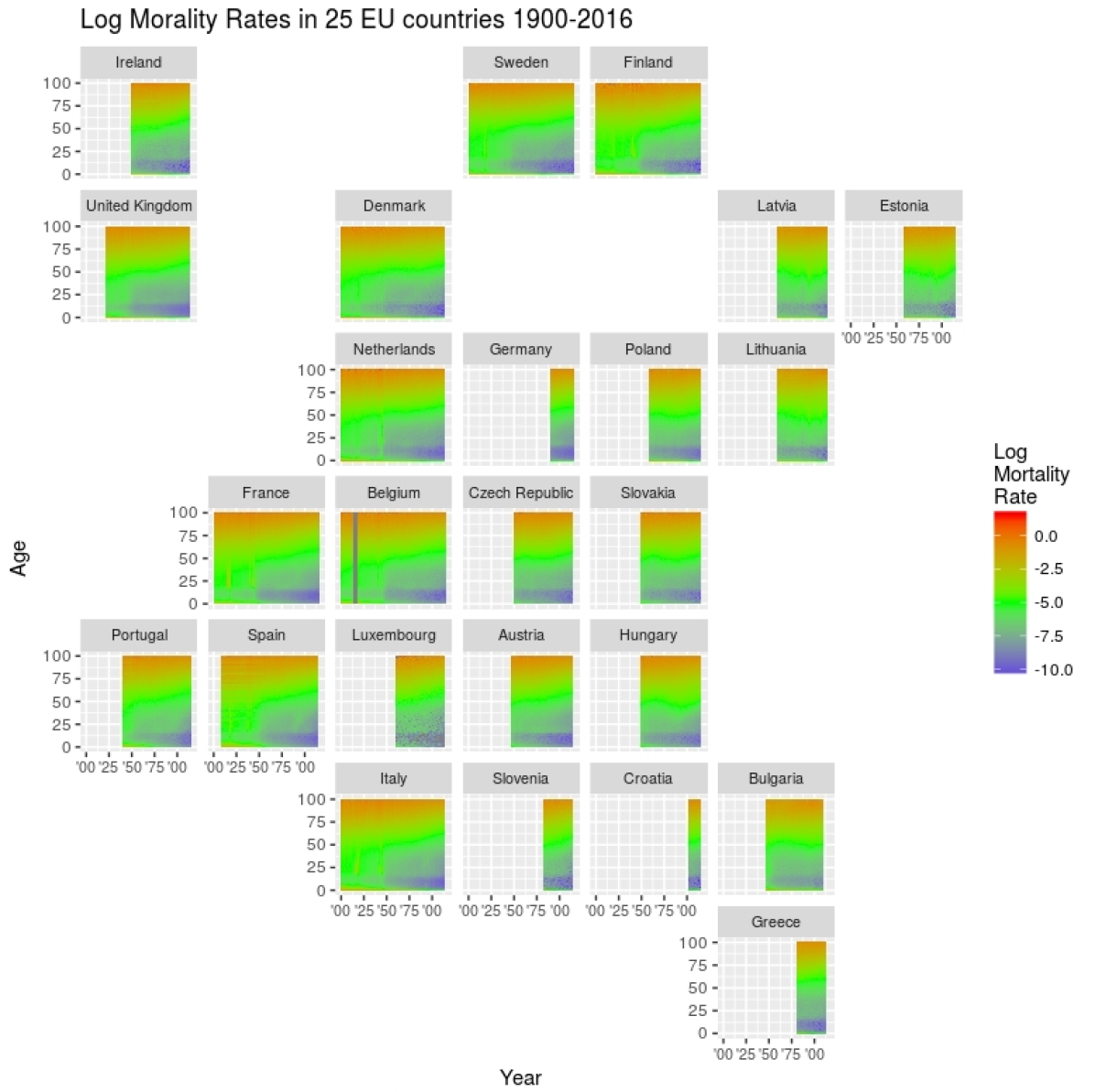
Figure 1: Single age-year log all cause mortality for 1900–2016, ages 0–100 in 25 EU member countries.

There are clear similarities in the mortality trends. Early childhood mortality rates are decreasing, and most countries show improvement in mortality rates for the middle aged. The toll of the two world wars is pronounced, with bright bands of higher mortality across all age groups in several countries. There is a general shift towards lower mortality in working years after WWII with wider understanding and usage of vaccines and antibiotics as well as further development of state-based public health initiatives. The changes in mortality rates also show some geographic patterns. For example, the bright green frontier of higher mortality shows a consistent change from ages 50 to 75 in northern, southern, and western Europe but is relatively flat in eastern Europe.

The remainder of this paper is as follows. In Section 2 we review the identification problem in univariate APC models and discuss stratified APC models based on multivariate GMRFs. The new stratified APC model is introduced in Section 3, with implementation details in Section 4. We conclude with the application to all-cause mortality in the EU in Section 5 and a discussion of other research directions.

2 Background

2.1 Univariate APC models

Let $\mathbf{Y}=\{y_{ij}:i=1,\dots,A;j=1,\dots,T\}$ be a matrix of the number of cases in each of $A$ age groups and $T$ periods, and let $\mathbf{N}=\{N_{ij},i=1,\dots,A;j=1,\dots,T\}$ be the number of person-years at risk in each age group and time period. The cohort index $k$ is a function of age and period. When the age scale and time scale are the same (e.g., 5 year age groups and 5 year time intervals), then $k=A-i+j$ so that $k\in\{1,\dots,A+T-1\}$. In this paper we assume $y_{ij}\sim\mathsf{Poi}(N_{ij}\exp\mu_{ij})$, but the methods described can easily be used for other likelihoods. For example, for country-level all-cause mortality it may be reasonable to assume a Gaussian likelihood directly on the log mortality rates. The basic APC model for the log rate is (Clayton and Schifflers, 1987)

$$\log\mathsf{E}\left[\frac{y_{ij}}{N_{ij}}\right] =\mu_{ij}=\delta+\alpha_{i}+\beta_{j}+\gamma_{k}.$$ (1)

It is well known that the parameters in (1) are not directly interpretable as log relative risks because the model is over parametrized. Kuang et al. (2008) and Nielsen and Nielsen (2014), following Carstensen (2007), define this identifiability issue from a group theoretic perspective. The overall mean, as given in (1), is invariant to a translation on each set of effects and the addition of a linear trend in the age, period, and cohort parameters. Let $\mathcal{G}=\{g:g\boldsymbol{\theta}=(g\delta,g\boldsymbol{\alpha},g\boldsymbol{\beta},g\boldsymbol{\gamma})\}$ be a group of transformations where

$$g\delta = \delta-a-b-c+(A-1)d$$ (2)

$$g\boldsymbol{\alpha} = \left\{\alpha_{i}+a+(i-1)d\right\}_{i=1}^{A}$$ (3)

$$g\boldsymbol{\beta} = \left\{\beta_{j}+b-(j-1)d\right\}_{j=1}^{T}$$ (4)

$$g\boldsymbol{\gamma} = \left\{\gamma_{k=A-i+j}+c+(A-i+j-1)d\right\}_{i=1,j=1}^{i=A,j=T}$$ (5)

for any real numbers $a,b,c,$ and $d$. An interpretation of these numbers is that $a$, $b$, and $c$ are the overall levels of the age, period, cohort effects, respectively, and $d$ is the linear trend. The log rates are invariant with respect to these transformations. That is, for any $g\in\mathcal{G}$, $\mu_{ij}(g\boldsymbol{\theta})=\mu_{ij}(g\delta,g\alpha_{i},g\beta_{j},g\gamma_{k})=\mu_{ij}(\delta,\alpha_{i},\beta_{j},\gamma_{k})=\mu_{ij}(\boldsymbol{\theta})$:

$$\mu_{ij}(g\delta,g\alpha_{i},g\beta_{j},g\gamma_{k}) =\left(\delta-a-b-c-(A-1)d\right)+\left(\alpha_{i}+a+(i-1)d\right)$$

$$\,+\left(\beta_{j}+b-(j-1)d\right)+\left(\gamma_{k}+c+(A-i+j-1)d\right)$$

$$=\delta+\alpha_{i}+\beta_{j}+\gamma_{k}$$

$$=\mu_{ij}(\delta,\alpha_{i},\beta_{j},\gamma_{k}).$$

Typically the distribution of the observed data only depends on the age, period, and cohort parameters through the log rates. Thus the likelihood itself is invariant with respect to $\mathcal{G}$, and the full set of age, period, and cohort effects is not identifiable. More specifically, the overall level and linear trend in each set of effects are unidentifiable.

The issue of overall levels can be resolved uncontroversially in the univariate case with sum-to-zero constraints on the $\boldsymbol{\alpha}$, $\boldsymbol{\beta}$ and $\boldsymbol{\gamma}$ terms or by setting one category from each of these terms as the reference category. The second form of non identifiability arises because of the linear dependence between the age, period, and cohort indices, and there is no genuine solution to this problem though many in the literature have proposed adding constraints based on expert knowledge or convenient mathematical criteria (Fienberg, 2013). However, seemingly innocuous differences in the choice of such constraints can yield contradictory estimates of $\boldsymbol{\alpha}$, $\boldsymbol{\beta}$, and $\boldsymbol{\gamma}$.

2.2 Existing stratified APC models

An important extension of the basic APC model is to incorporate time-independent factors (strata) such as gender, region, or disease subtype. Let $r,r=1,\dots,R$ represent the index for strata, then the most general stratified APC model is

$$\mu_{ijr}=\delta_{r}+\alpha_{ir}+\beta_{jr}+\gamma_{kr},$$

so that the full parameter space $\boldsymbol{\Theta}$ is an $R\times 2(A+T)$ matrix with rows $(\delta_{r},\boldsymbol{\alpha}_{r},\boldsymbol{\beta}_{r},\boldsymbol{\gamma}_{r})$, $r=1,\dots,R$. One can separately apply a stratum-specific $g\in\mathcal{G}$ with $(a_{r},b_{r},c_{r},d_{r})$ to each row of $\boldsymbol{\Theta}$ without changing the log rates. Hence, $4R$ constraints are required to produce identifiable age, period, and cohort effects.

In a stratified APC model, certain cross-strata relative risks are identifiable up to a multiplicative constant if one set of effects is shared across strata. Specifically, for the other two sets of non-shared effects, trends in relative risks within the same time index but between strata are identifiable. For example, suppose the age effects are shared across strata (that is $\alpha_{ir}=\alpha_{i}$ for all $i$), then the unidentifiable level of the age effects and the unidentifiable linear trend are common to all strata: $a_{r}=a$ and $d_{r}=d$. The relative risk between strata $r_{1}$ and $r_{2}$ in time period $1$ is $\exp(\beta_{1r_{1}}-\beta_{1r_{2}})$. For two transformations defined by $(a,b_{r_{1}},c_{r_{1}},d)$ and $(a,b_{r_{2}},c_{r_{2}},d)$ this becomes

$$g_{1}\beta_{jr_{1}}-g_{2}\beta_{jr_{2}} =\beta_{jr_{1}}-\beta_{jr_{2}}+(b_{r_{1}}-b_{r_{2}})$$

$$\left[\exp(g_{1}\beta_{jr_{1}}-g_{2}\beta_{jr_{2}})\right] =\exp(\beta_{jr_{1}}-\beta_{jr_{2}})\exp(b_{r_{1}}-b_{r_{2}}).$$

Thus, in a plot of $\exp(\beta_{jr_{1}}-\beta_{jr_{2}})$ against $j$, the y-axis scaling is ambiguous (i.e., can be multiplied by any positive number), but the overall shape–including the existence and direction of linear trends–can be ascertained. Note that all of the identifiability problems discussed in Section 2.1 still persist within each stratum.

In Riebler and Held (2010) and Riebler et al. (2012a), the age effects are assumed to be the same across regions; in Riebler et al. (2012b), period effects were shared, again across regions; and in Papoila et al. (2014), cohort effects are share by gender. For example, the model in Riebler et al. (2012a) is

$$\mu_{ijr}=\delta_{r}+\alpha_{i}+\beta_{jr}+\gamma_{kr}.$$

The authors fit these models in a Bayesian framework using correlated intrinsic Gaussian Markov random fields priors on each set of time effects. Specifically the prior on the age effects and the marginal prior on the period and cohort effects for a given region is a second order random walk (RW-2) prior, and the cross correlation between the effects of different regions is incorporated using a Kronecker-structured covariance.

With a single, univariate intrinsic GMRF prior, sum-to-zero constraints are typical because the precision matrix is not full rank (Rue and Held, 2005), and in the GMRF-based multivariate APC models, there are many sum-to-zero constraints. Thus these multivariate RW-2 models seem avoid the issue of multiplicative ambiguity in the cross-strata relative risks, when in fact they are only identifiable conditional on an implicit choice of $b_{r}$’s and $c_{r}$’s made by these constraints. While the sum-to-zero constraints were uncontroversial in the univariate APC model, they can give the misleading impression that these cross-strata relative risks are fully identifiable.

3 Methodology

Smith and Wakefield (2016) explored Bayesian inference for an APC parameterization based on non-linear aspects of the age, period, and cohort effects, and in this section we review this model and extend to the hierarchical setting using matrix-normal priors.

3.1 Canonical parameterisation

Kuang et al. (2008), Nielsen and Nielsen (2014), and Martínez Miranda et al. (2015) put forward a univariate APC model for data with equal-width age and time intervals in terms of three initial log rates and a full set of second differences in the age, period, and cohort effects. There exists a unique, full rank design matrix, $M$, such that the vector of log rates $\boldsymbol{\mu}$ can be expressed as

$$\boldsymbol{\mu}=M\boldsymbol{\xi},\,\xi=\{\mu_{{ijk}_{1}},\mu_{{ijk}_{2}},\mu_{{ijk}_{3}},\Delta^{2}\boldsymbol{\alpha},\Delta^{2}\boldsymbol{\beta},\Delta^{2}\boldsymbol{\gamma}\}.$$ (6)

Here $\boldsymbol{\xi}$ is a vector of length $2(A+T)-4$, which is exactly the number of parameters in (1) less the number of free constants defining the group $\mathcal{G}$.

The entries in $M$ are determined by the choice of coordinates for the base rates $\mu_{{ijk}_{1}},\mu_{{ijk}_{2}},\mu_{{ijk}_{3}}$. Kuang et al. (2008) and Nielsen and Nielsen (2014) chose three initial time points using age-cohort indices (i.e., $\mu_{ijk}=\mu_{ik}$), and Martínez Miranda et al. (2015) use age-period indexing (i.e., $\mu_{ijk}=\mu_{ij}$). The three pair of indices must be chosen so that they define a triangle rather than a line. So $\{\mu_{11},\mu_{12},\mu_{13}\}$ is not an acceptable choice, but $\{\mu_{11},\mu_{12},\mu_{21}\}$ is in either coordinate system. For simplicity, we assume this requirement is satisfied and use the more general notation $\{\mu_{{ijk}_{1}},\mu_{{ijk}_{2}},\mu_{{ijk}_{3}}\}=\{\mu_{0}^{1},\mu_{0}^{2},\mu_{0}^{3}\}$.

If we choose the largest or smallest values of $i$ and $j$ or $k$, the baseline rates are in the corners of the data array. For example, Martínez Miranda et al. (2015) use the earliest periods and the oldest age groups:

$$\{\mu_{0}^{1},\mu_{0}^{2},\mu_{0}^{3}\}=\{\mu_{A1},\mu_{A-1,1},\mu_{A2}\}.$$

Alternatively, we can choose values in the middle of the array. Suppose $A$ is odd and let $U=(A+1)/2$ be the middle age index. Nielsen (2015) suggests using

$$\{\mu_{0}^{1},\mu_{0}^{2},\mu_{0}^{3}\}=\{\mu_{UU},\mu_{U+1,U},\mu_{U,U+1}\}$$

in age-cohort coordinates. A further option is to parametrize in terms of one initial point and two differences:

$$\boldsymbol{\mu}=M^{\star}\boldsymbol{\xi}^{\star},\,\boldsymbol{\xi}^{\star}=\{\mu_{0}^{1},\mu_{0}^{2}-\mu_{0}^{1},\mu_{0}^{3}-\mu_{0}^{1},\Delta^{2}\boldsymbol{\alpha},\Delta^{2}\boldsymbol{\beta},\Delta^{2}\boldsymbol{\gamma}\},$$ (7)

where ‘$\star$’ emphasizes that the design matrix in 6 and 7 are different in the first three columns, but the estimates of the second differences are identical: $\boldsymbol{\xi}[4:(2(A+T)-4)]=\boldsymbol{\xi}^{\star}[4:(2(A+T)-4)]$. An example design matrix is in the Supplementary Materials.

The first three terms in this parametrization define a simple linear model for changes in disease (log) rates over time with an intercept ($\mu_{0}^{1}$) and two slopes ($\mu_{0}^{2}-\mu_{0}^{1}$ and $\mu_{0}^{3}-\mu_{0}^{1}$). The remaining terms then describe the non-linear deviations from this simple specification. For example, assuming $\{\mu_{0}^{1},\mu_{0}^{2},\mu_{0}^{3}\}=\{\mu_{UU},\mu_{U,U+1},\mu_{U+1,U}\}$, the log rates in age-cohort indices are

$$\mu_{ik}= \mu_{UU}+(i-U)(\mu_{U+1,U}-\mu_{UU})+(k-U)(\mu_{U,U+1}-\mu_{UU})$$ (8)

$$\qquad\qquad+M_{[,-(1:3)]}\boldsymbol{\xi}_{[-(1:3)]}.$$

This is similar to the models discussed in (Rosenberg and Anderson, 2011), which include an intercept, two slopes (net drift and either the longitudinal or cross-sectional age trend), and non linear terms. The curvature terms (second differences) can also be interpreted as accelerations in the trends along the three time scales (Clayton and Schifflers, 1987).

3.2 Matrix variate normal priors for multi-way data

Smith and Wakefield (2016) introduced a Bayesian hierarchical model based on the parameterization in Section 3.1 by incorporating uniform priors on the three initial points and Gaussian priors on the vectors of second differences. The main benefit of Bayesian inference in that paper was to shrink the curvature terms (in particular the cohort terms) that are not be well estimated by maximum likelihood. Here we extend this model by using matrix-normal priors, which will again provide some penalization but also allow for pooling of information across strata.

The matrix normal prior is a common tool for analyzing multi-way data including multivariate spatial data (Gelfand and Vounatsou, 2003; Knorr-Held, 2000; Smith et al., 2015) as well as mortality data (Fosdick and Hoff, 2014). Let $\mathbf{X}\sim\mathsf{MN}(\boldsymbol{\nu},\boldsymbol{\Sigma}_{C},\boldsymbol{\Sigma}_{R})$ denote the matrix normal distribution with separable covariance structure and mean $\boldsymbol{\nu}$ (Dawid, 1981). This means $\mathsf{vec}\left({\mathbf{X}}\right)\sim\mathsf{N}\left(\mathsf{vec}(\boldsymbol{\nu}),\boldsymbol{\Sigma}_{C}\otimes\boldsymbol{\Sigma}_{R}\right)$, where ‘$\mathsf{vec}(\cdot)$’ stacks the columns of a matrix into a single vector and ‘$\otimes$’ is the Kronecker product. Here $\boldsymbol{\Sigma}_{C}$ is the column covariance matrix describing correlation arising from the feature indexing the columns (e.g., the strata), and similarly the row covariance matrix $\boldsymbol{\Sigma}_{R}$ describes the correlation arising the feature indexing the rows. A mean of $\boldsymbol{\nu}=0$ is typical when using the matrix normal distribution as a prior for latent random effects.

The separable covariance structure in the matrix normal is computationally convenient because only the individual row and column covariance matrices and never the full covariance matrix appear in calculations. Suppose $n_{r}$ and $n_{c}$ are the row and column dimensions, then the probability density function for the matrix normal can be written as

$$\left(2\pi|\boldsymbol{\Sigma}_{C}\otimes\boldsymbol{\Sigma}_{R}|\right)^{-1/2}\exp\left\{-\mathsf{vec}(\mathbf{X}-\boldsymbol{\nu})^{\prime}(\boldsymbol{\Sigma}_{C}\otimes\boldsymbol{\Sigma}_{R})^{-1}\mathsf{vec}(\mathbf{X}-\boldsymbol{\nu})/2\right\}$$

$$=\left(2\pi|\boldsymbol{\Sigma}_{C}|^{n_{r}}|\boldsymbol{\Sigma}_{R}|^{n_{c}}\right)^{-1/2}\exp\left\{-\mathsf{tr}\left[\Sigma_{C}^{-1}(\mathbf{X}-\boldsymbol{\nu})^{\prime}\Sigma_{R}^{-1}(\mathbf{X}-\boldsymbol{\nu})\right]/2\right\}.$$

3.3 An identifiable stratified APC model

Let the vectors $\mathbf{y}_{r}$ and $\mathbf{N}_{r}$, $r=1,\dots R$ represent the numbers of deaths and population sizes for the $r^{\text{th}}$ stratum. We assume the counts follow a Poisson distribution with rates broken into the age, period, and cohort effects according to the identifiable parameterization in 3.1:

$$\mathbf{y}_{r} \sim\mathsf{Poi}(\mathbf{N}_{ijr}\exp(M\boldsymbol{\xi}_{r}))$$

$$\boldsymbol{\xi}_{r} =\{\mu_{0r}^{1},\mu_{0r}^{2},\mu_{0r}^{3},\Delta^{2}\boldsymbol{\alpha}_{r},\Delta^{2}\boldsymbol{\beta}_{r},\Delta^{2}\boldsymbol{\gamma}_{r}\}$$

$$\equiv\{\boldsymbol{\xi}_{0r},\boldsymbol{\xi}_{\alpha r},\boldsymbol{\xi}_{\beta r},\boldsymbol{\xi}_{\gamma r}\}$$

We organize the second differences and baseline rates into matrices. For example, we combine the $\boldsymbol{\xi}_{\alpha r}$’s to get an $(A-2)\times R$ matrix: $\boldsymbol{\Xi}_{\alpha}$ where

$$\boldsymbol{\Xi}_{\alpha[ir]}=\Delta^{2}\alpha_{i+2,r}$$

and similarly define $\boldsymbol{\Xi}_{0},\boldsymbol{\Xi}_{\beta},\boldsymbol{\Xi}_{\gamma}$. We use the matrix normal prior to allow for correlation between the accelerations across strata:

$$\boldsymbol{\Xi}_{\phi} \sim\mathsf{MN}\left(0;\tau^{-1}_{\phi}\mathcal{I},\Sigma_{s}(\rho_{\phi})\right),\quad\phi=\alpha,\beta,\gamma.$$

The first covariance matrix is the scaled identity matrix, meaning that, within a stratum, the second differences or log baseline rates are independent. The second variance matrix encodes the cross-strata correlation, the strength of which may be governed by a parameter $\rho$. Note that we cannot have a scale parameter for both covariance matrices because only the product of these two is identifiable. In this model, the separable covariance structure means assuming that the covariance in the curvatures factors into a purely between-strata portion and a purely between-time portion. For the baseline points, we still use a matrix normal prior but include the mean as a parameter instead of assuming a zero mean:

$$\boldsymbol{\Xi}_{0} \sim\mathsf{MN}\left(\boldsymbol{\nu}_{0};\tau^{-1}_{0}\mathcal{I},\Sigma_{s}(\rho_{0})\right).$$

Three possible choices for $\Sigma_{s}$ are considered here: independent, exchangeable, and spatial. The first two are straightforward. For independence we have $\Sigma_{s}=\mathcal{I}$ and for the exchangeable model

$$\Sigma_{s}[ij]=\begin{cases}1&i=j,\\ \rho&i\neq j\end{cases}\quad\rho\in\left(-\frac{1}{R-1},1\right).$$

Where the strata represent geographic regions, a covariance matrix encoding larger correlations for near-by areas and smaller correlations for areas far away from each other is of interest. A classical choice is to base this around the neighborhood structure of the regions via an adjacency matrix $W$:

$$W_{ij}=\begin{cases}1,&j\in\text{nbhd}(i)\\ 0,&j\not\in\text{nbhd}(i).\end{cases}$$

where $j\in\text{nbhd}(i)$ means areas $i$ and $j$ share a border. This forms the basis of the intrinsic conditional-autoregressive (ICAR) model with precision matrix $Q_{s}=D-W,$ where D is a diagonal matrix with entries equal to the row sums of W. Often independent random effects are used alongside spatial random effects to account for both structured and unstructured correlation.

Here we follow the recommendations of Riebler et al. (2016) and use the so-called BYM2 model where the random effect is the weighted sum of an independent and a spatial component, with the spatial component scaled by $\sigma^{2}_{\text{ref}}$, the geometric mean of the marginal variances under $Q_{s}$ as defined above. This scaling is important because the prior variance of the random effects depends on the neighborhood structure in the ICAR prior (Sørbye and Rue, 2014). Under the BYM2 model, the cross-stratum correlation matrix is

$$\Sigma_{s}(\rho)=(1-\rho)\mathcal{I}-\rho Q_{\star}^{-},\quad\rho\in(0,1)$$

where $Q_{\star}^{-}$ is the generalized inverse of $Q_{s}$, scaled by $\sigma^{2}_{\text{ref}}$. An alternative to this areal approach is to construct a spatial covariance matrix based on the distance between some measure of the center of each region, but we do not pursue this option here.

The stratified APC model proposed here has some similarities with the multivariate RW-2 models discussed in Section 2.2. We can re-write a second-order random walk for regular time intervals as

$$\boldsymbol{\alpha} \sim\text{RW-2}(\tau_{\alpha}=1)$$

$$\implies\alpha_{i}|\boldsymbol{\alpha}_{-i}\sim N\left(\frac{2}{3}(\alpha_{i-1}+\alpha_{i+1})-\frac{1}{6}(\alpha_{i-2}+\alpha_{i+2}),\frac{1}{6}\right),\,2<i<A-2$$

$$\implies\pi(\boldsymbol{\alpha})\propto\exp\left(\frac{-1}{2}\sum_{i=3}^{A}(\alpha_{i}-2\alpha_{i-1}+\alpha_{i-2})^{2}\right)$$

$$\implies\Delta^{2}\alpha_{i}\sim N(0,\mathcal{I}),\,i=3,\dots,A.$$

Hence the multivariate GMRF priors discussed earlier can also be viewed as matrix-normal priors on second differences (or first difference if the GMRF is a RW-1 model). There are also overlaps in the cross-strata correlations considered: the correlation in Riebler et al. (2012a) is the same as our exchangeable model.

The advantage of specifying the model only in terms of parameters that are identifiable (as we do here) is that we do not mistakenly report contrasts that are only identified based on implicit constraints. To investigate $\exp(\beta_{jr_{1}}-\beta_{jr_{2}})$ against $j$, we must specify $b_{r_{1}}$ and $b_{r_{2}}$, reminding us that the relative risk is only identifiable up to a multiplicative factor.

4 Implementation

4.1 Model selection

We consider modifications from the full stratified APC model by allowing some parameters to be shared across regions. We consider six models as summarized in Table 1. This is not an exhaustive list of all possible combinations of effects being shared or heterogeneous. Instead we prioritize sharing the baseline rates and age curvature with the rationale that age is a surrogate for biological processes that are less susceptible to environmental effects. We select a model using WAIC, which estimates the out of sample prediction error based on the log point-wise posterior predictive density of the observed data with a penalty to avoid over fitting (Gelman et al., 2014).

Table 1: Summary of models to be considered. A ✓means that parameter is constant across the strata. For example, in M5, $\boldsymbol{\xi}_{r0}=\boldsymbol{\xi}_{0}$, but all of the other effects are allowed to vary.

	M1	M2	M3	M4	M5	M6
$\boldsymbol{\xi}_{0}$	✓	✓	✓	✓	✓
$\boldsymbol{\xi}_{\alpha}$	✓	✓	✓	✓
$\boldsymbol{\xi}_{\beta}$	✓	✓
$\boldsymbol{\xi}_{\gamma}$	✓		✓

For each of the models where the parameters are allowed to vary across strata, we also have a choice of correlation structure as outline in Section 3.2. For simplicity we assume the same structure holds for each set of parameters, though we allow different hyper-parameter values. For each model in Table 1 (except M1), we consider three versions of the correlation structure: independent, exchangeable, and BYM2. Thus the total number of models to choose from is 16.

4.2 Software

We have chosen to fit the hierarchical APC model with integrated nested Laplace approximations (INLA) as implemented in the R-INLA package (Rue et al., 2009). INLA is a well-established method for fast and accurate approximations of the marginal posterior distributions for random effects and hyper-parameters when there are many latent Gaussian random effects, as is the case here.

Though we can view this model as a generalized linear mixed model with random slopes, there are some complications because we want to share the variance for certain blocks of the parameters. We handle this using by passing in the relevant rows of $M$ via the $A$ matrix option in control.predictor, where the $M$ matrix itself is constructed via the apc package (Nielsen, 2016). The Kronecker structured covariance is available using the group option. The full code for implementing all of the models considered in this paper is in the Supplementary Materials.

5 Application to the Human Mortality Database

We apply this model to mortality rates in 25 European Union (EU) countries from the Human Mortality Database introduced in Section 1. We fit our stratified APC models to these data from 1925-2015 and ages 0-80 aggregating by 5-year age and period groups for a total of 17 age groups, 18 periods, and 34 cohorts. For the BYM2 models, the concept of an adjacency is tricky because not all countries in Europe are covered in our example. We consider all countries that share a boundary to be adjacent but add in additional links along major rail, ferry, or road routes to create a single connected component. See the Supplementary Materials for a map of the study region with addition links. While it is not strictly necessary to create a single connected component, without these additional links we had four connected components, three of which only had two members (UK-Ireland, Sweden-Finland, Greece-Bulgaria). A priori the random effects for these disconnected pairs would not benefit from pooling of information across space, so we connected them to the remaining 19 areas.

5.1 Hyper-prior distributions

We follow the recommendations in Smith and Wakefield (2016) by specifying exponential priors on the precisions where the scale parameter is chosen based on a prior ‘confidence interval’ for predictions in the age, period, or cohort effects. If we believe that the residual for predicting for the next period effect under the prior ($\beta_{T+1}-\mathsf{E}[\beta_{T+1}\mid\beta_{1},\dots,\beta_{T}]$) to be no more than $\epsilon_{\beta}$ in absolute value $100\cdot(1-q)$% of time, then this implies the rate in the hyper-prior for $\tau_{\beta}$ should be $(\epsilon_{\beta}/t_{1-q/2,\text{df}=2})^{2}/2$. For the application in Section 5, we take $q=0.05$ and $\epsilon_{\alpha}=\log(1.2)=\epsilon_{\beta}=\log(1.1)$, $\epsilon_{\gamma}=\log(1.01)$. For M6 (where the baseline rates are allowed to vary), we use $\epsilon_{0}=\log(1.05)$. In this example, we have more time periods than in the examples considered by Smith and Wakefield (2016), so we expect less sensitivity to these priors. For the correlation parameters, we use $\log((1+\rho(25-1))/(1-\rho))\sim N(0,\sqrt{5})$ in the exchangeable case, and for the BYM2 model we use the penalized complexity prior from Riebler et al. (2016) assuming $Pr(\rho<0.5)=0.5$. These are the default settings for these models in R-INLA.

For $\boldsymbol{\xi}_{0}$, we use the baseline and two-slopes version from equation 8. In this case, $U=9$ so the intercept is the log all-cause mortality rate for 40-45 year olds in 1925-1930 and the two slopes are the log relative risk between this group and the same cohort when aged 45-50 as well as the same initial group compared to the next cohort at the same age. In the case of all-cause mortality, we have substantial prior knowledge of the base-line rates. Thus we depart from the recommendation of Smith and Wakefield (2016) and prefer to use an informative prior on $\boldsymbol{\nu}_{0}$, the population averaged baseline effects:

$$\boldsymbol{\nu}_{0}\sim N(v=\{\log(0.005),0.3,-0.1\},S=\text{diag}(1,0.1,0.1)).$$

This corresponds to a prior belief that the mortality of the baseline group is 5 per 1000 person years (95% prior interval 0.7 to 35.5), a 35% increase in risk for the age slope (27% decrease to 151% increase), and a 10% decrease in risk for the cohort slope (51% decrease to 68% increase). These values are loosely based on data from Switzerland, which is in the HMD but not included in this example because Switzerland is not in the EU. For Switzerland the observed values are $\hat{v}=\{\log(0.0065),0.256,-0.105\}$. In M6, $\boldsymbol{\nu}_{0}$ is a matrix with identical columns.

One may question why the prior variances for $\boldsymbol{\nu}_{0}$ are so small here. We followed the suggestions of Gabry et al. (2018) to assess the multivariate properties of the prior specification by checking that at least some simulations from the prior predictive distribution of $y$ were consistent with our expectations for real data. With wider priors on $\boldsymbol{\nu}_{0}$, the simulated data were orders of magnitude larger than is sensible (e.g., everyone in the population would have to die multiple times). Using the prior above, we did not have this issue, and there is still plenty of mass in the prior on extreme log rates. Under all 3 correlation structures, the maximum simulated count is greater than the observed maximum for the HMD data about 75% of the time, and the simulated minimum is less than the observed minimum about 60% of the time.

5.2 Results

We begin by fitting all 16 models from Section 4.1. The WAIC for each model is shown in Table 2. The four non-spatial models allowing the age, period, and cohort curvatures to differ by location are clearly superior. The best fitting model according to WAIC allows all of the parameter blocks to vary by location (M6) with some pooling of information via an exchangeable correlation structure.

Table 2: WAIC values for the 16 candidate models. A lower WAIC value indicates that a model has lower estimated out of sample prediction errors.

	IID	Exchangeable	BYM2
M1	5107697.20	–	–
M2	5456311.16	5455501.60	6344619.42
M3	4223834.56	4223592.08	6595823.26
M4	3908640.41	3907772.54	6335372.21
M5	2882880.75	2881512.50	6265486.50
M6	2760168.21	2758382.19	6239374.61

Table 3 show the posterior medians along with upper and lower limits of 95% credible intervals for the precisions (expressed as standard deviations), correlation parameters and mean baseline parameters ($\boldsymbol{\nu}_{0}$) for the top four models. The estimates across the four models are broadly consistent. The only major difference is the age slope $(\mu_{U+1,U}-\mu_{UU})$ is smaller when the baseline rate and slopes are allowed to vary. We also note that the width of the credible intervals is largest in M6-exchangeable model, which is expected given that this model has the largest number of hyper-parameters. Figure 2 shows the fitted (posterior medians) versus observed log rates for M6-exchangeable. There is some lack of fit in many countries for the smallest rates, and similar results were seen for the other three models.

Table 3: Parameter (posterior medians and with upper and lower limits of 95% credible intervals) for the top four models identified by WAIC.

	Independent		Exchangeable
	M5	M6	M5	M6
$\boldsymbol{\nu}_{0}[1]$	-4.95 (-4.96, -4.94)	-4.99 (-5.07, -4.91)	-4.95 (-4.96, -4.94)	-4.99 (-5.08, -4.91)
$\boldsymbol{\nu}_{0}[2]$	0.26 (0.26, 0.27)	0.31 (0.25, 0.36)	0.26 (0.26, 0.27)	0.31 (0.24, 0.38)
$\boldsymbol{\nu}_{0}[3]$	-0.089(-0.096,-0.083)	-0.091(-0.15,-0.034)	-0.088(-0.095,-0.081)	-0.088(-0.16,-0.018)
$\tau^{-1/2}_{\alpha}$	0.66 (0.62, 0.71)	0.66 (0.62, 0.71)	0.60 (0.45, 0.82)	0.60 (0.45, 0.82)
$\tau^{-1/2}_{\beta}$	0.095 (0.088, 0.1)	0.091 (0.084, 0.098)	0.10 (0.09, 0.12)	0.10 (0.086, 0.12)
$\tau^{-1/2}_{\gamma}$	0.064 (0.060, 0.068)	0.060 (0.057, 0.064)	0.064 (0.060, 0.069)	0.061 (0.056, 0.066)
$\tau^{-1/2}_{0}$		0.12 (0.10, 0.15)		0.12 (0.096, 0.14)
$\rho_{\alpha}$			0.97 (0.94, 0.98)	0.97 (0.95, 0.99)
$\rho_{\beta}$			0.47 (0.32, 0.65)	0.51 (0.36, 0.68)
$\rho_{\gamma}$			0.20 (0.12, 0.31)	0.22 (0.14, 0.34)
$\rho_{0}$				-0.024 (-0.041, 0.15)

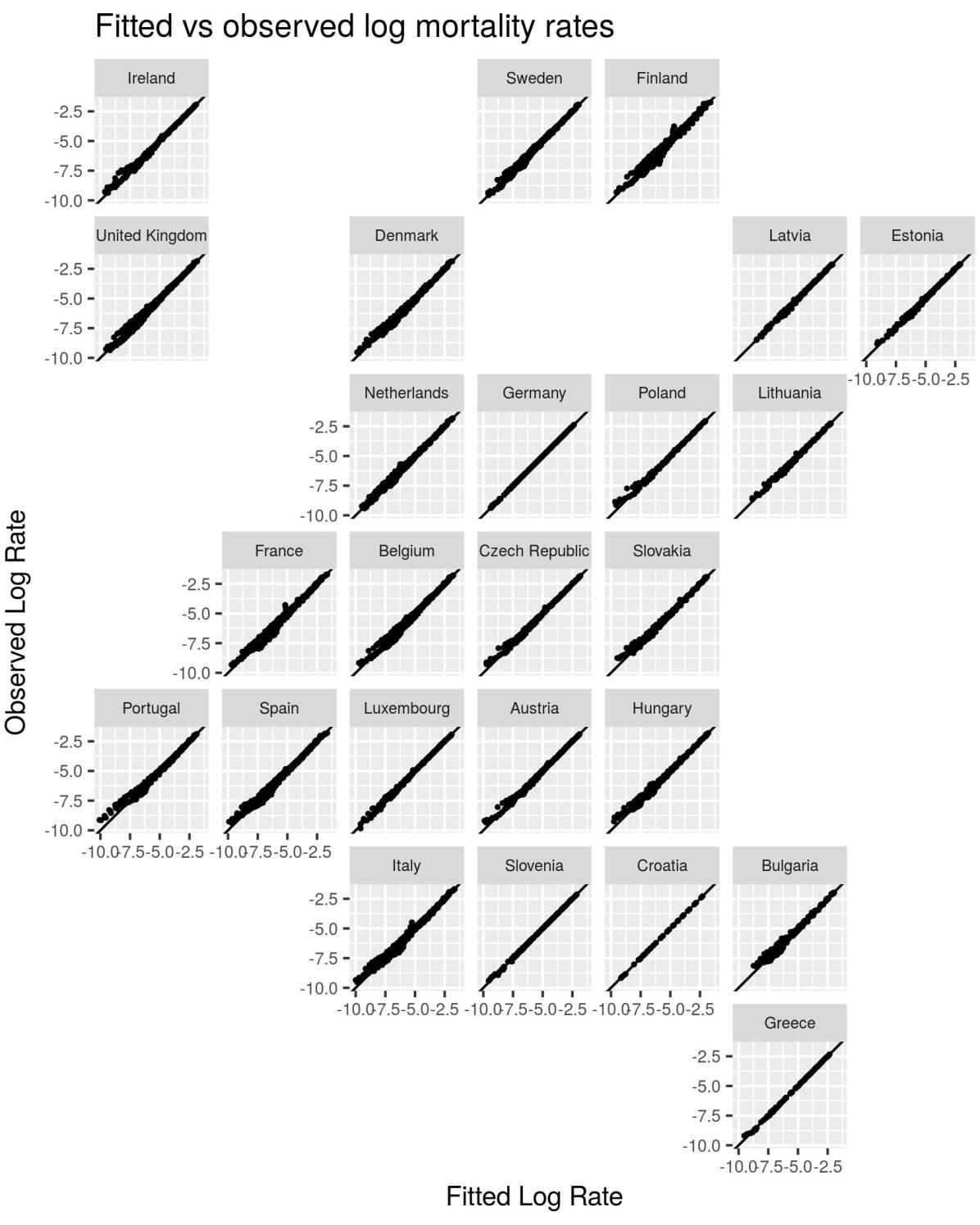
Figure 2: Fitted vs observed log mortality rates in 25 EU member countries. The fitted rates are based on the posterior medians from the M6-Exchangeable model.

For the remainder of this section we concentrate on the estimates from the top model overall (M6-exchangeable). In this model, the posterior median for the population-averaged mortality rate in the baseline group (40-45 year olds in 1925-1930) is $6.8$ death per 1000 person years (95% CrI: $6.2$ – $7.4$). The posterior median for the age slope, parameterized as the difference in log mortality between the baseline group and the same cohort when aged 45-50 is $0.31$, indicating a $36$% increase in the morality rate (95% CrI: $27$% – $46$%). The posterior median for the cohort slope, parameterized as the difference in log mortality between the baseline group and the next cohort at the same age is $-0.088$, indicating an $8$% decrease in risk (95% CrI: $15$% – $2$%).

The country-level baseline and slopes are moderately heterogeneous, but the deviations from the population averages are not significantly correlated. The range of posterior medians for the baseline rates is $4.6$ to $9.6$, with the highest risk in France, Spain and Finland and the lowest risk in the Netherlands (see Figure 3). In eastern Europe, the deviations from the expected log baseline rate and slopes are the smallest, which is not surprising given that there is substantial missing data here in the early periods where $\{\mu_{0}^{1},\mu_{0}^{2},\mu_{0}^{3}\}$ are located.

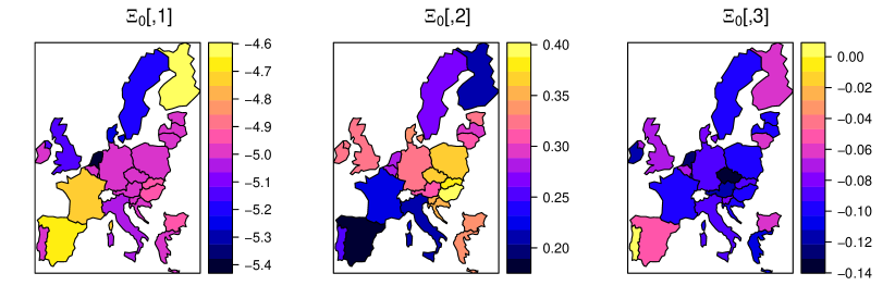
Figure 3: Posterior medians of $\boldsymbol{\Xi}_{0}$ for the M6-Exchangeable model.

These three terms define a simple linear model for the time trend in each countries, and the remaining variance hyper-parameters describe the variance and correlation of non-linear deviations from this simple paradigm. The age curvature terms have the largest standard deviation ($0.60(0.45-0.82)$) and the largest correlation ($0.97(0.95-0.99)$). This is not surprising because we know the relationship between age and mortality usually has a non linear ‘J’ shape. Further we expect the age effects to be consistent across countries because they are surrogates for processes that are less susceptible to environmental differences.

We can get a sense of the age effects by plotting the fitted rates across the age groups for a given period (i.e., cross-sectionally) or for a given cohort (i.e., longitudinally). We show the fitted cross-sectional age trends for 1970 (the middle time period) across all countries in Figure 4 (left). The countries are ordered west to east by centroid. We see the characteristic ‘J’ shape and broadly the same curvature except that a few eastern European countries have somewhat straighter curves between 15 and 40. It is important to remember that differences in fit here are combinations of age and cohort effects and not solely due to differences in the age curvatures.

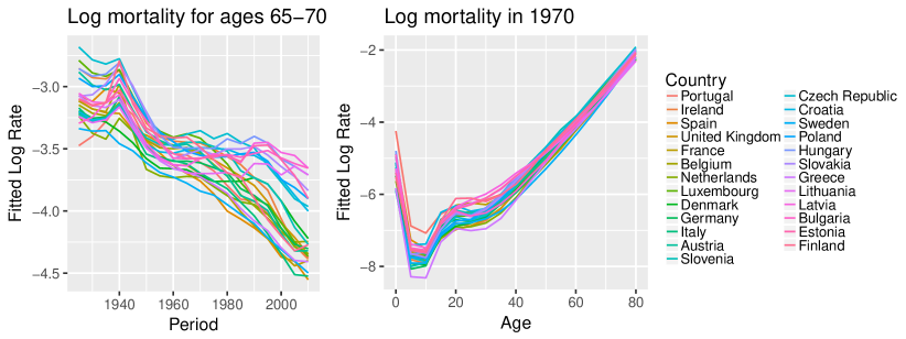
Figure 4: Posterior medians of log rates in the 65-70 age group over period (left) and in 1970 across age groups (right) by country from the M6-exchangeable model.

The period and cohort deviations are smaller and less correlated than the age curvatures. Thus we expect more heterogeneity in the trends of of disease along these two time scales than along the age time scale. We can get a sense of the net effect of both the period and cohort effects, sometimes called drift, by plotting the fitted log rates for one age group across time. Figure 4 (right) shows this plot for the 65-70 age group, across all countries. Pre 1960 the curves are very similar with a sharp peak in 1940 (WWII) and then steadily decreasing risk. The homogeneity in these earl years likely arises from the extent of missing data rather than genuine similarity. There is continued improvement in western Europe from 1960 onward which does not seem to start in eastern Europe until 1985. Once again we remind the reader that differences in fitted rates seen here are the net effects of period and cohort and not purely down to period effects.

5.3 Hindcast for Germany 1960-1990

As an additional check on the models, we imputed the mortality counts for Germany and compared against the true values reconstructed by combining the counts for East Germany (GDR) and West Germany (FRG). The HMD has data on unified Germany from 1990, which is the second shortest data record in this example after Croatia. However, there are separate records for the GDR and FRG in the HMD, with the GDR records going back to 1960.

While the WIAC used in the previous section gives an estimate of the out of sample prediction, comparing hindcasts of Germany mortality rates from 1960-1990 gives us an additional opportunity to test the predictive power of our models. For each of the M6 models, we sample from the posterior distribution of the log rates using the inla.posterior.sample function and then sample the number of deaths from the Poisson distribution. We use the denominators ($N$’s) reconstructed from the HMD in this process, which may not be available in general.

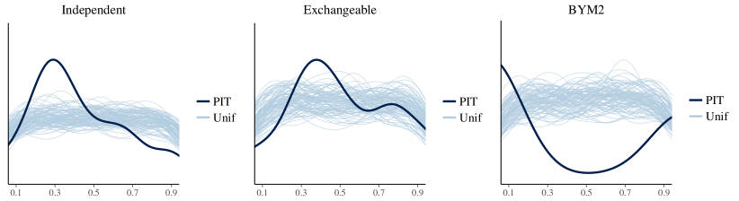
Figure 5: Smoothed PIT histograms and histograms of simulated uniforms for M6 under each correlation model.

One way to assess these predictions is using probability integral transform (PIT) histograms (Held et al., 2010). For each age-period combination, we evaluate the empirical cumulative distribution function of the posterior samples at the observed count. If the posterior distribution for the missing data is a well calibrated prediction, then these proportions are approximately uniformly distributed. Figure 5 shows smoothed PIT histograms versus smoothed histograms for random samples from $\mathsf{U}(0,1)$ for each correlation structure. There is miss calibration in all three models, but the exchangeable model is clearly better calibrated than the other models. The shape of the BYM2 histogram also gives us some insight into why the spatial models performed so poorly in earlier comparisons. The $\cup$ shape means the posterior predictive distributions are under-dispersed (too narrow).

6 Discussion

This article presents a Bayesian stratified APC model that allows for pooling of information on non-linear aspects of the age, period, and cohort effects across strata using matrix normal priors with separable covariance structures. We considered several cross-correlation models and put forward tools for selecting between more parsimonious versions of the full model. This approach is based on a fully identifiable parameterization, thus avoiding the major drawback of stratified APC models based on multivariate GMRFs.

To our knowledge, the only other developments towards a multivariate APC model outside the GMRF framework are from Chernyavskiy et al. (2017), who allow for heterogeneity in the intercept and two trends but not the curvature terms as we did here. There are however numerous age-space-time or age-strata-time models where only period effects are included. For example in a recent paper Goicoa et al. (2017) use splines to capture age-time trends in mortality and (in the most complicated model considered by the authors) there is a common age-time response surface along with region-specific age-time surfaces. Because there are only two time scales in an age-space-time model, we can directly interpret the age-time effects; whereas, in the model proposed in this paper, we can only interpret the accelerations along these scales.

In the application to the HMD data, the independent and exchangeable models with heterogeneous period curvatures only (M2) were superior to the models with heterogeneous cohort curvatures only (M3), suggesting that if one of the three time scales had to be dropped in favor of a more interpretable model, it should be cohort. However, the model with heterogeneity in both period and curvature (M4) improved on both of these, indicating that a full APC model is appropriate.

Interestingly the spatial model in our application performed poorly compared to the exchangeable and independent cross-correlation models. One possible explanation for this is that the data are unbalanced in a spatially-structured way: the shortest data series are clustered in eastern Europe. Thus pooling information based on the neighborhood structure in the BYM2 model is not advantageous since there is little signal to draw on in the first place. Understanding the role of spatially-structured missingness more generally is an avenue for future research.

The parameterization on which we based our stratified model in Section 3 is limited to data with equal-width age and time intervals. Relaxing this assumption is an important direction for future development. Though 5-year age groups are standard, the time periods to which providers of official mortality data aggregate differ considerably with data sometime provided at shorter (1-year) or longer (10-year) intervals. Even if all agencies report on 5-year time periods, the intervals may be misaligned. In spatial misalignment problems, one approach is to specify a model on smallest possible units (e.g., single age-year intervals here) and then aggregate the mean as appropriate (Gelfand, 2010). If we follow this suggestion for the stratified APC model, the mean for the observed counts would no longer be log linear in the random effects. This poses additional computational challenges, and ascertaining which parameters remain identifiable is not straightforward.

Supplementary materials

• Supplement A: Design matrix for APC models, directions for downloading data from the HMD and code for the analysis carried out Section 5. (SupplementA.Rmd/.pdf)

• Supplement B: folder of model scripts called in the .Rmd file (SupplementB.zip)

References

- Carstensen [2007] B. Carstensen. Age–period–cohort models for the Lexis diagram. Statistics in Medicine, 26:3018–3045, 2007.
- Chernyavskiy et al. [2017] P. Chernyavskiy, M.P. Little, and P.S. Rosenberg. A unified approach for assessing heterogeneity in age–period–cohort model parameters using random effects. Statistical methods in medical research, page 0962280217713033, 2017.
- Clayton and Schifflers [1987] D. Clayton and E. Schifflers. Models for temporal variation in cancer rates. I: age–period and age–cohort models. Statistics in medicine, 6:449–467, 1987.
- Dawid [1981] A.P. Dawid. Some matrix-variate distribution theory: notational considerations and a Bayesian application. Biometrika, 68:265–274, 1981.
- Fienberg [2013] S.E. Fienberg. Cohort analysis’ unholy quest: A discussion. Demography, 50:1981–1984, 2013.
- Fosdick and Hoff [2014] B.K. Fosdick and P.D. Hoff. Separable factor analysis with applications to mortality data. The Annals of Applied Statistics, 8:120–147, 2014.
- Gabry et al. [2018] J. Gabry, D. Simpson, A. Vehtari, M. Betancourt, and A. Gelman. Visualization in Bayesian workflow. ArXiv e-prints, arXiv:1709.01449v4, 2018.
- Gelfand and Vounatsou [2003] A. Gelfand and P. Vounatsou. Proper multivariate conditional autoregressive models for spatial data analysis. Biostatistics, 4:11–25, 2003.
- Gelfand [2010] A.E. Gelfand. Misalgined spatial data: The change of support problem. In A.E. Gelfand, P. Diggle, P. Guttorp, and M. Fuentes, editors, Handbook of spatial statistics, pages 517 – 539. CRC press, 2010.
- Gelman et al. [2014] A. Gelman, J.B. Carlin, H.S. Stern, D.B. Dunson, A. Vehtari, and D.B. Rubin. Bayesian Data Analyis, Third Edition. CRC Press, 2014.
- Goicoa et al. [2017] T. Goicoa, A. Adin, J. Etxeberria, A.F. Militino, and M.D. Ugarte. Flexible Bayesian P-splines for smoothing age-specific spatio-temporal mortality patterns. Statistical methods in medical research, page 0962280217726802, 2017.
- Held et al. [2010] L. Held, B. Schrödle, and H. Rue. Posterior and cross-validatory predictive checks: a comparison of MCMC and INLA. In T. Kneib and G. Tutz, editors, Statistical modelling and regression structures, pages 91–110. Springer, 2010.
- Human Mortality Database, University of California, Berkeley and Max Planck Institute for Demographic Research (Germany)() [USA] Human Mortality Database, University of California, Berkeley (USA) and Max Planck Institute for Demographic Research (Germany). Available at http://www.mortality.org or http://www.humanmortality.de (data downloaded in September 2017).
- Knorr-Held [2000] L. Knorr-Held. Bayesian modelling of inseparable space-time variation in disease risk. Statistics in Medicine, 19:2555–2567, 2000.
- Kuang et al. [2008] D. Kuang, B. Nielsen, and J.P. Nielsen. Identification of the age-period-cohort model and the extended chain-ladder model. Biometrika, 95:979–986, 2008.
- Martínez Miranda et al. [2015] M.D. Martínez Miranda, B. Nielsen, and J.P. Nielsen. Inference and forecasting in the age–period–cohort model with unknown exposure with an application to mesothelioma mortality. Journal of the Royal Statistical Society: Series A, 278:29–55, 2015.
- Nielsen [2015] B. Nielsen. apc: An R package for age-period-cohort analysis. R Journal, 7, 2015.
- Nielsen [2016] B. Nielsen. apc: Age-Period-Cohort Analysis, 2016. URL https://CRAN.R-project.org/package=apc. R package version 1.3.
- Nielsen and Nielsen [2014] B. Nielsen and J.P. Nielsen. Identification and forecasting in mortality models. The Scientific World Journal, 2014.
- Papoila et al. [2014] A.L. Papoila, A. Riebler, A. Amaral-Turkman, R. São-João, C. Ribeiro, C. Geraldes, and A. Miranda. Stomach cancer incidence in Southern Portugal 1998–2006: A spatio-temporal analysis. Biometrical Journal, 56:403–415, 2014.
- Riebler and Held [2010] A. Riebler and L. Held. The analysis of heterogeneous time trends in multivariate age–period–cohort models. Biostatistics, 11:57–69, 2010.
- Riebler et al. [2012a] A. Riebler, L. Held, and H. Rue. Estimation and extrapolation of time trends in registry data – borrowing strength from related populations. Annals of Applied Statistics, 6:304–333, 2012a.
- Riebler et al. [2012b] A. Riebler, L. Held, H. Rue, and M. Bopp. Gender-specific differences and the impact of family integration on time trends in age-stratified Swiss suicide rates. Journal of the Royal Statistical Society: Series A (Statistics in Society), 175:473–490, 2012b.
- Riebler et al. [2016] A. Riebler, S.H. Sørbye, D. Simpson, and H. Rue. An intuitive Bayesian spatial model for disease mapping that accounts for scaling. Statistical Methods in Medical Research, 25:1145–1165, 2016.
- Rosenberg and Anderson [2011] P.S. Rosenberg and W.F. Anderson. Age-period-cohort models in cancer surveillance research: ready for prime time? Cancer Epidemiology Biomarkers & Prevention, 20:1263–1268, 2011.
- Rosenberg et al. [2014] P.S. Rosenberg, D.P. Check, and W.F. Anderson. A web tool for age–period–cohort analysis of cancer incidence and mortality rates. Cancer Epidemiology Biomarkers & Prevention, 23:2296–2302, 2014.
- Rue and Held [2005] H. Rue and L. Held. Gaussian Markov Random Fields: Theory And Applications (Monographs on Statistics and Applied Probability). Chapman & Hall/CRC, 2005. ISBN 1584884320.
- Rue et al. [2009] H. Rue, S. Martino, and N. Chopin. Approximate Bayesian inference for latent Gaussian models using integrated nested Laplace approximations (with discussion). Journal of the Royal Statistical Society, Series B, 71:319–392, 2009.
- Schwartz [1986] L. Schwartz. A history of Russian and Soviet censuses. In R.S. Clem, editor, Research Guide to the Russian and Soviet Censuses, pages 48–69. Cornell University Press, 1986.