Probabilistic AND-OR Attribute Grouping for Zero-Shot Learning

Abstract

In zero-shot learning (ZSL), a classifier is trained to recognize visual classes without any image samples. Instead, it is given semantic information about the class, like a textual description or a set of attributes. Learning from attributes could benefit from explicitly modeling structure of the attribute space. Unfortunately, learning of general structure from empirical samples is hard with typical dataset sizes.

Here we describe LAGO, a probabilistic model designed to capture natural soft and-or relations across groups of attributes. We show how this model can be learned end-to-end with a deep attribute-detection model. The soft group structure can be learned from data jointly as part of the model, and can also readily incorporate prior knowledge about groups if available. The soft and-or structure succeeds to capture meaningful and predictive structures, improving the accuracy of zero-shot learning on two of three benchmarks.

Finally, LAGO reveals a unified formulation over two ZSL approaches: DAP (Lampert et al., 2009) and ESZSL (Romera-Paredes & Torr, 2015). Interestingly, taking only one singleton group for each attribute, introduces a new soft-relaxation of DAP, that outperforms DAP by $\scriptstyle\sim$40%.

Figure 1: Classifying a bird species based on attributes from (Wah et al., 2011). The Mourning Warbler can be distinguished from other species by a combination of a grey head and olive-green underparts. Both human raters and machine learning models may confuse semantically-similar attributes like olive or green wings. These attribute naturally cluster into ”OR” groups, where we aim to recognize this species if the wing is labeled as either green or olive. The LAGO model (Eq. 4) weighs attributes detection, inferring classes based on within-group soft-OR and across-groups soft-AND. In general, OR-groups include alternative choices of a property (wing_color:{red, olive, green}) and soft-OR allows to weigh down class-irrelevant attributes (here, wing:red).

1 INTRODUCTION

People can easily learn to recognize visual entities based on a handful of semantic attributes. For example, we can recognize a bird based by its visual features (long beak, red crown), or find a location based on a language description (a 2-stories brick town house). Unfortunately, when training models that use such semantic features, it is typically very hard to leverage semantic information effectively. With semantic features, the input space has rich and complex structure, due to nontrivial interactions and logical relations among attributes. For example, the color of petals may be red or blue but rarely both, while the size of a bird is often not indicative of its color.

Taking into account the semantics of features or attributes becomes crucial when no training samples are available. This learning setup, called zero-shot learning (ZSL) is the task of learning to recognize objects from classes wihtout any image samples to train on. (Lampert et al., 2009; Farhadi et al., 2009; Palatucci et al., 2009; Xian et al., 2017b). Instead, learning is based on semantic knowledge about the classes (Socher et al., 2013; Elhoseiny et al., 2013; Berg et al., 2010), like in the case of attribute sharing (Lampert et al., 2009, 2014). Here, the training and test classes are accompanied by a set of predefined attributes, like ”A Zebra is striped” or ”A Hummingbird has a long bill”, provided by human experts. Then, a classifier is trained to detect these attributes in images (Ferrari & Zisserman, 2008), and test images are classified by detecting attributes and mapping to test classes based on the expert knowledge.

Broadly speaking, approaches to ZSL with attributes can be viewed as learning a compatibility function $f(Attr(image),Attr(class))$ between an attribute-based representation of an image and an attribute-based representation of classes (Romera-Paredes & Torr, 2015; Akata et al., 2016; Frome et al., 2013; Akata et al., 2015). Here, the attributes of a class are provided by (possibly several) experts, the image attributes are automatically detected, and one aims to learn a scoring function that can find the class whose attributes are most compatible with an image. Most ZSL approaches represent attributes as embedded in a “flat” space, Euclidean or Simplex, but flat embedding may miss important semantic structures. Other studies aimed to learn a structured scoring function, for example using a structured graphical model over the attributes (Wang & Ji, 2013). Unfortunately, learning complex structures of probabilistic models from data requires large datasets, which are rarely available.

Here we put forward an intermediate approach: We use training classes to learn a simple structure that can capture simple (soft) and-or logical relations among attributes. More concretely, after mapping an image to attributes, we aggregate attributes into groups using a soft OR (weighted-sum), and then score a class by taking a soft AND (product of probabilities) over group activations (Figure 2). While the attributes are predefined and provided by experts, the soft groups are learned from the training data.

The motivation for learning the and-or structure becomes clear when observing how attributes tend to cluster naturally into semantically-related groups. For example, descriptions of bird species in the CUB dataset include attributes like {wing-color:green, wing-color:olive, wing-color:red} (Wah et al., 2011). As another example, animal attributes in (Lampert et al., 2009) include {texture:hairless, texture:tough-skin}. In these two examples, the attributes are semantically related, and raters (or a classifier) may mistakenly interchange them, as evident by how Wikipedia describes the Mourning Warbler (Figure 1) as having “olive-green underparts”. In such cases, it is natural to model attribute structure as a soft OR relation over attributes (“olive” or “green”) in a group (“underparts”). It is also natural to apply a soft AND relation across groups, since a class is often recognized by a set of necessary properties.

We describe LAGO, ”Learning Attribute Grouping for 0-shot learning”, a new zero-shot probabilistic model that leverages and-or semantic structure in attribute space. LAGO achieves new state-of-the-art result on CUB and AWA2(Lampert et al., 2009), and competitive performance on SUN (Patterson & Hays, 2012). Interestingly, when considering two extremes of attribute grouping, LAGO becomes closely related to two important ZSL approaches. First, in the case of a single group (all OR), LAGO is closely related to ESZSL (Romera-Paredes & Torr, 2015). At the opposite extreme where each attribute forms a singleton group, (all AND), LAGO is closely related to DAP (Lampert et al., 2009). LAGO therefore reveals an interesting unified formulation over seemingly unrelated ZSL approaches.

Our paper makes the following novel contributions. We develop a new probabilistic model that captures soft logical relations over semantic attributes, and can be trained end-to-end jointly with deep attribute detectors. The model learns attribute grouping from data, and can effectively use domain knowledge about semantic grouping of attributes. We further show that it outperforms competing methods on two ZSL benchmarks, CUB and AWA2, and obtain comparable performance on another benchmark (SUN). Finally, LAGO provides a unified probabilistic framework, where two previous important ZSL methods approximate extreme cases of LAGO.

2 RELATED WORK

Zero-shot-learning with attributes attracted significant interest recently (Xian et al., 2017b; Fu et al., 2017). One influential early works is Direct Attribute Prediction (DAP), which takes a Bayesian approach to predict unseen classes from binary attributes (Lampert et al., 2009). In DAP, a class is predicted by the product of attribute-classifier scores, using a hard-threshold over the semantic information of attribute-to-class mapping. DAP is related in an interesting way to LAGO. We show below that DAP can be viewed as a hard-threshold special case of LAGO where each group consists of a single attribute.

Going beyond a flat representation of attributes, several studies modeled structure among attributes. Wang & Ji (2013) learned a Bayesian network over attribute space that captures object-dependent and object-independent relationships. Jiang et al. (2017) learned latent attributes that preserve semantics and also provide discriminative combinations of given semantic attributes. Structure in attribute space was also used to improve attribute prediction: Jayaraman et al. (2014) leveraged side information about semantic relatedness of attributes in given groups and proposed a multi-task learning framework, where same-group attributes are encouraged to share low-level features. In Park & Zhu (2015); Park et al. (2017), the authors propose an AND-OR grammar model (Zhu & Mumford, 2006), to jointly represent both the object parts and their semantic attributes within a unified compositional hierarchy. For that, they decompose an object to its constituent parts with a parse tree. In their model, the tree nodes (the parts) constitute an AND relation, and each OR-node points to alternative sub-configurations

Our approach resonates with Markov Logic Networks (MLN), (Richardson & Domingos, 2006) and Probabilistic Soft Logic (PSL), (Kimmig et al., 2012; Bach et al., 2017). It shares the idea of modeling domain knowledge using soft logical relations. Yet, LAGO formulation provides a complementary point of view: (1) LAGO derivation reveals the probabilistic meaning of every soft weight of the logical relation Eq. (3), and offers a principled way to set priors when deriving the soft logical expression. (2) The step-by-step derivation reveals which approximations are taken when mapping features to classes with soft logical relations. (3) Logical relations are incorporated in LAGO as part of an end-to-end deep network. PSL and MLN use Markov random field with logical relations as constraints or potentials.

The study of ZSL goes beyond learning with attributes (Changpinyo et al., 2016; Tsai et al., 2017b; Morgado & Vasconcelos, 2017; Rohrbach et al., 2011; Al-Halah & Stiefelhagen, 2015; Zhang et al., 2017; Ye & Guo, 2017; Tsai et al., 2017a; Xu et al., 2017; Li et al., 2017; Zhang & Koniusz, 2018). Recently, Zhang & Koniusz (2018) described a kernel alignment approach, mapping images to attribute space such that projected samples match the distribution of attributes in terms of a nonlinear kernel. Another popular approach to ZSL learns a bi-linear compatibility function $F(\mathbf{x},y;W)=\theta(\mathbf{x})^{\top}W\phi(y)$ to match visual information $\theta(\mathbf{x})$ with semantic information $\phi(y)$ (Romera-Paredes & Torr, 2015; Akata et al., 2016; Frome et al., 2013; Akata et al., 2015). In this context, most related to our work is ESZSL (Romera-Paredes & Torr, 2015), which uses a one-hot encoding of class labels to define a mean-squared-error loss function. This allows ESZSL to have a closed-form solution where reaching the optimum is guaranteed. We show below that ESZSL is closely related to a special case of LAGO where all attributes are assigned to a single group.

The current work focuses on a new architecture for ZSL with attributes. Other aspects of ZSL, including feature selection (Guo et al., 2018) and data augmentation (Mishra et al., 2018; Arora et al., 2018; Xian et al., 2018), can improve accuracy significantly, but are orthogonal to the current work.

Figure 2: LAGO network architecture (Sec 3). Image features are extracted by a deep ConvNet and fed to a FC sigmoid layer ($\sigma$) that outputs a prediction score $p(a_{m}|x)$ for each binary attribute $a_{m}$. Attribute scores are grouped into $K$ soft groups, and mapped to a set $\{g_{k,z}\}$ of $K\times|Z|$ binary classifiers, according to a soft-OR Eq. (3). Finally, a class is computed by the soft product of all group-scores for that class, approximating a conjunction (AND). In the diagram, each colored circle represents a classifier score for a separate class.

3 A PROBABILISTIC AND-OR MODEL

The Problem Setup:

Following the notations of (Lampert et al., 2009), we are given a set of labeled training images $(\mathbf{x}_{i}\in\mathcal{X},z_{i}\in\mathcal{Z})$ drawn from a distribution $D$. Each image $\mathbf{x}$ is accompanied by a vector of binary attributes $\mathbf{a}\in\{True,False\}^{|A|}$, $\mathbf{a}=(a_{1},\dots,a_{m},\dots,a_{|A|})$, where $a_{m}=True$ if the image has attribute $a_{m}$. We are also given a set of class ”descriptions” in the form class-conditioned attribute distribution $p(\mathbf{a}|z)$. In practice, the descriptions are often collected separately per attribute ($m$), and only the marginals $p(a_{m}|z)$, $\forall m$ are available.

At training time, we aim to learn a classifier that predicts a class $z$ of an image $\mathbf{x}$ by first learning to predict the attributes $\mathbf{a}$, and then use $p(a_{m}|z)$, $\forall m$ to predict a class $z$ based on the attributes.

At inference time (the zero-shot phase), we are given images $\mathbf{x}$ from new unseen classes with labels $y\in\mathcal{Y}$, and together with their class descriptions ${p}(a_{m}|y)$, $\forall m$. We similarly predict the class $y$ by first predicting attributes $\mathbf{a}$ and then use $p(a_{m}|z)$, $\forall m$ to predict a class $y$ based on the attributes.

Model Overview:

The LAGO model (Figures 1, 2) learns a soft logical AND-OR structure over semantic attributes. It can be viewed as a concatenation of three mapping steps $\mathcal{X}\rightarrow\mathcal{A}\rightarrow\mathcal{G}\rightarrow\mathcal{Z}$. First, attribute predictions: an image $\mathbf{x}$ is mapped to a vector of attribute detection probabilities $f^{1}_{W}:\mathcal{X}\rightarrow\mathcal{A}$, $\mathcal{A}=[0,1]^{|A|}$. The mapping parameters $W$ determine the weights of the attribute detectors and are learned from labeled training data. Second, weighted-OR group scores: Attribute probabilities are mapped to $K$ groups. Each group calculates a class-dependent weighted-OR over the $|Z|$ classes $f^{2}_{{U},{V}}:\mathcal{A}\rightarrow\mathcal{G}$, $\mathcal{G}=[0,1]^{K\times|Z|}$. The mapping parameters ${U}$ are the distributions $p(\mathbf{a}|z)$ provided with each class; The mapping parameters ${V}$ determine how attributes are grouped and are learned from data. Last, soft-AND group conjunction: Per-group scores are mapped to class detection probabilities by a soft-AND, approximating group conjunction. $f^{3}:\mathcal{G}\rightarrow\mathcal{Z}$, $\mathcal{Z}=[0,1]^{|Z|}$. The parameters $W,{V}$ are learned jointly to minimize a regularized loss with a regularizer $R$:

$$\min_{W,{V}}\quad loss(f^{3}(f^{2}_{{U},{V}}(f^{1}_{W}(\mathbf{x}_{i}))),z_{i})+R(W,{V})\quad.\vspace{-5pt}$$ (1)

The key idea in the proposed approach is to define a layer of binary classifiers $g_{k,z}$, each evaluating a class $z$ based only on a subset $G_{k}\subset\mathcal{A}$ of attributes. For example, for bird-species recognition, one classifier may detect a Mourning Warbler based on wing colors and another based on bill shapes. In this example, each of the classifiers output the probability $p(g_{k,z}=True|\mathbf{a})$ that the image has a Mourning Warbler, but based on different subsets of attributes. The partition of attributes to subsets is shared across classes, hence with $K$ subsets we have $K\times|Z|$ binary classifiers. We also define $\mathbf{a}_{k}$ to be the vector of attributes detections for $G_{k}$, $\mathbf{a}_{k}\in\{T,F\}^{|G_{k}|}$. For clarity, we first derive the algorithm for groups that are fixed (not learned) and hard (non-overlapping). Section 3.1 then generalizes the derivation to soft learned groups.

Consider now how we compute $p(g_{k,z}\!=\!T|\mathbf{x})$. According to the Markov property, it equals $\sum_{\mathbf{a}_{k}}p(g_{k,z}|\mathbf{a}_{k})p(\mathbf{a}_{k}|\mathbf{x})$, but computing this sum raises several challenges. First, since the number of possible patterns in a group grows exponentially with its size, the summation becomes prohibitively large when attribute groups are large. Second, estimating $p(g_{k,z}|\mathbf{a}_{k})$ from data may also be hard because the number of samples is often limited. Finally, description information is often available for the marginals only, $(z,a_{m})$, rather than the full distribution $(z,\mathbf{a}_{k})$. We now discuss a model that addresses these constraints.

The Within-Group Model $\mathcal{A}\rightarrow\mathcal{G}$:

We now show how one can compute $p(g_{k,z}|\mathbf{x})$ efficiently by treating attributes within group as obeying a soft OR relation. As discussed above, OR relations are in good agreement with how real-world classes are described using hard semantic attributes, because a single property (a group like beak-shape) may be mapped to several semantically-similar attributes (pointy, long).

Formally, we first define a complementary attribute per group, $\tilde{a_{k}}=\left(\mathop{\mathbin{\scalebox{1.5}{$\cup$}}}_{m\in G_{k}}a_{m}\right)^{c}$, handling the case where no attributes are detected or described, and accordingly define $G_{k}^{\prime}=G_{k}\mathop{\mathbin{\scalebox{1.5}{$\cup$}}}\tilde{a_{k}}$. We then use the identity ${p}(A)={p}(A,B)+{p}(A,B^{c})$ to partition ${p}(g_{k,z}\!=\!T|\mathbf{x})$ to a union (OR) of its contributions from each of its attributes. Specifically, ${p}(g_{k,z}\!=\!T|\mathbf{x})={p}(g_{k,z}\!=\!T,\mathop{\mathbin{\scalebox{1.5}{$\cup$}}}_{m\in G_{k}}a_{m}=T|\mathbf{x})+{p}(g_{k,z}\!=\!T,\tilde{a_{k}}=T|\mathbf{x})$ $={p}(\mathop{\mathbin{\scalebox{1.5}{$\cup$}}}_{m\in G_{k}^{\prime}}(g_{k,z}\!=\!T,a_{m}=T)|\mathbf{x})$. Using this equality and approximating attributes within a group as being mutually exclusive, we have

$${p}(g_{k,z}\!=\!T|\mathbf{x})\approx\sum_{m\in G_{k}^{\prime}}{p}(g_{k,z}\!=\!T,a_{m}=T|\mathbf{x}).$$ (2)

To rewrite this expression in terms of class descriptions $p(a_{m}|z)$ we take the following steps. First, the Markov chain $\mathcal{X}\rightarrow\mathcal{A}\rightarrow\mathcal{G}$ gives ${p}(g_{k,z}\!=\!T,a_{m}|\mathbf{x})$ $=$ ${p}(g_{k,z}\!=\!T|a_{m}){p}(a_{m}|\mathbf{x})$. Second, we note that by the definition of $g_{k,z}$, $p(g_{k,z}|\mathbf{a}_{k})=p(z|\mathbf{a}_{k})$, because $g_{k,z}$ is the classifier of $z$ based on $\mathbf{a}_{k}$. This yields ${p}(g_{k,z}\!=\!T,a_{m})={p}(z,a_{m})$ by marginalization. Applying Bayes to the last identity gives ${p}(g_{k,z}\!=\!T|a_{m})={{p}(a_{m}|z){p}(g_{k,z}\!=\!T)}/{{p}(a_{m})}$ (more details in Supplementary Material D.1). Finally, combining it with the expression for ${p}(g_{k,z}\!=\!T,a_{m}|\mathbf{x})$ and with Eq. (2) we can express ${p}(g_{k,z}\!=\!T|\mathbf{x})$ as

$${p}(g_{k,z}\!=\!T|\mathbf{x}){}\approx\\ {p}(g_{k,z}\!=\!T)\sum\limits_{m\in G_{k}^{\prime}}\frac{{p}(a_{m}=T|z)}{{p}(a_{m}=T)}{p}(a_{m}=T|\mathbf{x}).$$ (3)

Conjunction of Groups $\mathcal{G}\rightarrow\mathcal{Z}$:

Next, we derive an expression of the conditional probability of classes ${p}(z|\mathbf{x})$ using soft-conjunction of group-class classifiers $g_{k,z}$. Using the Markov property $\mathcal{X}\rightarrow\mathcal{A}\rightarrow\mathcal{G}\rightarrow\mathcal{Z}$, and denoting ${g_{1,z}\dots g_{K,z}}$ by $\mathbf{g}_{z}$, we can write
${p}(z|\mathbf{x})\!=\!\sum_{\mathbf{g}_{z}}{p}(z|\mathbf{g}_{z}){p}(\mathbf{g}_{z}|\mathbf{x})$. We show on Supplementary D.2, that making a similar approximation as in DAP (Lampert et al., 2009), for groups instead of attributes, yields Eq. (A.16): ${p}(z|\mathbf{x})\approx{p}(z)\prod_{k=1}^{K}\frac{{p}(g_{k,z}=T|\mathbf{x})}{{p}(g_{k,z}=T)}$. Combining it with Eq. (3), we conclude

$${p}(z|\mathbf{x}){}\approx\,\,\,\,{p}(z)\prod\limits_{k=1}^{K}\Big{[}\!\!\sum_{m\in G_{k}^{\prime}}\!\!\frac{{p}(a_{m}\!=\!T|z)}{{p}(a_{m}\!=\!T)}{p}(a_{m}\!\!=\!\!T|\mathbf{x})\Big{]}.$$ (4)

3.1 SOFT GROUPS:

The above derivation treated attribute groups as hard: deterministic and non-overlapping. We now discuss the more general case where attributes are probabilistically assigned to groups.

We introduce a soft group-membership variable $\Gamma_{m,k}={p}({m\in G_{k}^{\prime}})$, yielding a soft version of Eq. (3)

$${p}(g_{k,z}\!=\!T|\mathbf{x}){}\approx\\ {p}(g_{k,z}\!=\!T)\sum_{m=1}^{|\mathcal{A}|}\Gamma_{m,k}\frac{{p}(a_{m}=T|z)}{{p}(a_{m}=T)}{p}(a_{m}=T|\mathbf{x}),$$ (5)

where each row of $\Gamma$ represents a distribution over $K$ groups per attribute in the simplex $\Delta^{K}$. Hard grouping is a special case of this model where all probability mass is assigned to a single group for each row of $\Gamma$. The full derivation is detailed in Supplementary Material (D.3).

3.2 LEARNING

LAGO has three sets of parameters learned from data.

First, a matrix $W$ parametrizes the mapping $f^{1}_{W}:\mathbf{x}\rightarrow[0,1]^{|A|}$ from image features to attribute detection probabilities ${p}(a_{m}|\mathbf{x})$. This mapping is implemented as a fully-connected layer with sigmoid activation over image features extracted from ResNet-101.

Second, a matrix $U$, where its entry ${U}_{m,z}$ parametrizes the class-level description ${p}(a_{m}|z)$. When attribute ratings are given per image, we estimate ${U}$ using maximum likelihood from co-occurrence data over attributes and classes.

Third, a matrix ${V}_{|A|\times K}$ parametrizes the soft group assignments $\Gamma_{|A|\times K}$, such that each row $m$ maintains $\Gamma_{(m,:)}=\text{softmax}(\zeta{V}_{(m,:)})$, where $\zeta\in\mathbb{R}^{+}$ is a smoothing coefficient. This parametrization allows taking arbitrary gradient steps over ${V}$, while guaranteeing that each row of $\Gamma$ corresponds to a probability distribution in the simplex $\Delta^{K}$.

Since $W$ and ${V}$ are shared across all classes, they are learned over the training classes and transferred to the test classes at (zero-shot) inference time. They are learned end-to-end by applying cross-entropy loss over the outputs of Eq. (4) normalized by their sum across classes (forcing a unit sum of class predictions). As in (Romera-Paredes & Torr, 2015), the objective includes two regularization terms over $W$: A standard $L_{2}$ regularizer $||W||^{2}_{Fro}$ and a term $||W{U}||^{2}_{Fro}$, which is equivalent for an ellipsoid Gaussian prior for $W$. For the ”LAGO-Semantic-Soft” learning-setup (Section 4) we introduce an additional regularization term $||\Gamma_{({V})}-\Gamma_{({V}_{SEM})}||^{2}_{Fro}$, pushing the solutions closer to known semantic hard-grouping $\Gamma_{({V}_{SEM})}$. Finally, we optimize the loss:

$$L(W,{U},{V},Z,A,X){}=\text{CXE}_{{p}(z|\mathbf{x};W,{U},{V})}(X,Z)+\\ \alpha\text{BXE}_{{p}(a|\mathbf{x};W)}(X,A)+\beta||W||^{2}_{Fro}+\lambda||WS||^{2}_{Fro}+\\ \psi||\Gamma_{({V})}-\Gamma_{({V}_{SEM})}||^{2}_{Fro},$$ (6)

where CXE is the categorical cross-entropy loss for ${p}(z|\mathbf{x})$, BXE is the binary cross-entropy loss for ${p}(\mathbf{a}|\mathbf{x})$, $X,Z$ and $A$ denote the training samples, labels and attribute-labels. Per-sample attribute labels are provided as their empirical mean per class. In practice, we set $\alpha=0$ (See Section 4.2) and cross-validate to select the values of $\beta$, $\lambda$ and $\psi$ when relevant.

3.3 INFERENCE

At inference time, we are given images from new classes $y\in\mathcal{Y}$. As with the training data, we are given semantic information about the classes in the form of the distribution $p(a_{m}|y)$. In practice, we are often not given that distribution directly, but instead estimate it using maximum likelihood from a set of labeled attribute vectors.

To infer the class of a given test image $\mathbf{x}$, we plug $p(a_{m}|y)$ estimates instead of $p(a_{m}|z)$ in Eq. (4), and select the class $y$ that maximizes Eq. (4).

3.4 DAP, ESZSL AS SPECIAL CASES OF LAGO

LAGO encapsulates similar versions of two other zero-shot learning approaches as extreme cases: DAP (Lampert et al., 2009), when having each attribute in its own singleton group ($K=|A|$), and ESZSL (Romera-Paredes & Torr, 2015), when having one big group over all attributes ($K=1$).

Assigning each single attribute $a_{m}$ to its own singleton group reduces Eq. (4) to Eq. (A.26) (details in Supplementary D.4). This formulation is closely related to DAP. When expert annotations ${p}(a_{m}=T|z)$ are thresholded to $\{0,1\}$ and denoted by $a^{z}_{m}$, Eq. (A.26) become the DAP posterior Eq. (A.28). This makes the singletons variant a new soft relaxation of DAP.

At the second extreme (details in Supplementary D.4), all attributes are assigned to a single group, $K\!=\!1$. Taking a uniform prior for ${p}(z)$ and ${p}(a_{m})$, and replacing ${p}(a_{m}\!\!=\!\!T|\mathbf{x})$ with the network model $\sigma(\mathbf{x}^{\top}W)$, transforms Eq. (4) to ${p}(z|\mathbf{x})\!\!\propto\!\!\!\!\sum_{m=1}^{|A|}\sigma(\mathbf{x}^{\top}W){p}(a_{m}\!\!=\!\!T|z)$. Denoting ${U}_{m,z}\!\!=\!\!{p}(a_{m}\!\!=\!\!T|z)$, this formulation reveals that at the extreme case of $K\!=\!1$, LAGO can be viewed as a non-linear variant that is closely related to ESZSL: $Score(z|\mathbf{x})\!\!=\!\!\mathbf{x}^{\top}WU$, with same entries ${U}_{m,z}$.

4 EXPERIMENTS

Fair comparisons across ZSL studies tends to be tricky, since not all papers use a unified evaluation protocol. To guarantee an ”apple-to-apple” comparison, we follow the protocol of a recent meta-analysis by Xian et al. (2017b) and compare to the leading methods evaluated with that protocol: DAP (Lampert et al., 2009), ESZSL (Romera-Paredes & Torr, 2015), ALE (Akata et al., 2016), SYNC (Changpinyo et al., 2016), SJE (Akata et al., 2015), DEVISE (Frome et al., 2013), Zhang2018 (Zhang & Koniusz, 2018). Recent work showed that data augmentation and feature selection can be very useful for ZSL (Mishra et al., 2018; Arora et al., 2018; Xian et al., 2018; Guo et al., 2018). Since such augmentation are orthogonal to the modelling part, which is the focus of this paper, we do not use them here.

4.1 DATASETS

We tested LAGO on three datasets: CUB, AWA2 and SUN. First, we tested LAGO in a fine-grained classification task of bird-species recognition using CUB-2011 (Wah et al., 2011). CUB has 11,788 images of 200 bird species and a vocabulary of 312 binary attributes (wing-color:olive), derived from 28 attribute groups (wing-color). Each image is annotated with attributes generated by one rater. We used the class description $p(a_{m}|z)$ provided in the data. The names of the CUB attributes provide a strong prior for grouping (wing-color:olive, wing-color:red, …$\rightarrow$ wing-color:{olive, red, …}).

The second dataset, Animals with Attributes2 (AWA2), (Xian et al., 2017a) consists of 37,322 images of 50 animal classes with pre-extracted feature representations for each image. Classes and attributes are aligned with the class-attribute matrix of (Osherson et al., 1991; Kemp et al., 2006).We use the class-attribute matrix as a proxy for the class description $p(a_{m}|z)$, since human subjects in (Osherson et al., 1991) did not see any image samples during the data-collection process. As a prior over attribute groups, we used the 9 groups proposed by (Lampert, 2011; Jayaraman et al., 2014) for 82 of 85 attributes, like texture:{furry, hairless, …} and shape:{big, bulbus, …}. We added two groups for remaining attributes: world:{new-world, old-world}, smelly:{smelly}.

As the third dataset, we used SUN (Patterson & Hays, 2012), a dataset of complex visual scenes, having 14,340 images from 717 scene types and 102 binary attributes from four groups.

4.2 EXPERIMENTAL SETUP

We tested four variants of LAGO:
(1) LAGO-Singletons: The model of Eq. (4) for the extreme case using $K=|A|$ groups, where each attribute forms its own hard group.
(2) LAGO-Semantic-Hard: The model of Eq. (4) with hard groups determined by attribute names. As explained in Section 4.1 .
(3) LAGO-K-Soft: The soft model of Eqs.
4-5, learning $K$ soft group assignments with $\Gamma$ initialized uniformly up to a small random perturbation. $K$ is a hyper parameter with a value between $1$ and the number of attributes. It is chosen by cross-validation.
(4) LAGO-Semantic-Soft: The model as in LAGO-K-Soft, but the soft groups $\Gamma$ are initialized using the dataset-specific semantic groups assignments. These are also used as the prior $\Gamma_{SEM}$ in Eq. (6).

Importantly, to avoid implicit overfitting to the test set, we used the validation set to select a single best variant, so we can report only a single prediction accuracy for the test set. For reference, we provide detailed test results of all variants in the Supplementary Material, Table A.1 .

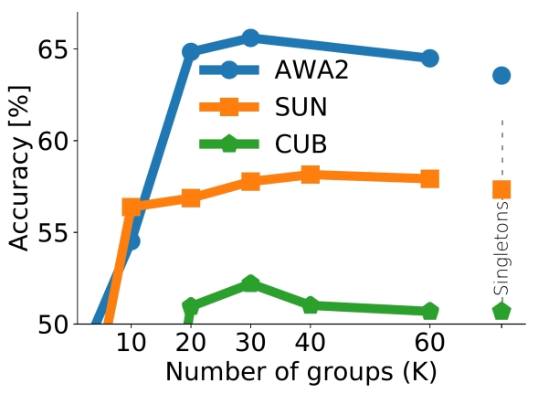
Figure 3: Learning K soft-group assignments: Validation-set accuracy for different number of groups ($K$) for the LAGO-K-Soft variant and of the LAGO-Singletons baseline. Here, no prior information is given about the groups, and the model successfully learns groups assignments from data, and better than the group-naive LAGO-Singletons baseline.

To learn the parameters $W,{V}$, we trained the weights with cross entropy-loss over outputs (and regularization terms) described in section 3.2. In the hard-group case, we only train $W$, while keeping ${V}$ fixed. We sparsely initialize ${V}$ with ones on every intersection of an attribute and its hard-assigned group and choose a high constant value for $\zeta$ ($\zeta=10$). Since the rows of $\Gamma$ correspond to attributes, it renders each row of $\Gamma$ as a unit mass probability on a certain group. In the soft-group case, we train $W,{V}$ alternately per epoch, allowing us to choose different learning rate for $W$ and ${V}$. For LAGO-K-Soft, ${V}$ was initialized with uniform random weights in [0, 1e-3], inducing a uniform distribution over $\Gamma$ up to a small random perturbation. For LAGO-Semantic-Soft, we initialized ${V}$ as in the hard-group case, and we also used this initialization for the prior ${V}_{SEM}$ Eq. (6).

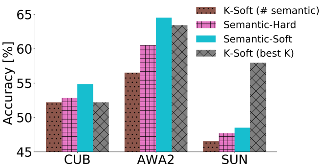
Figure 4: Validation accuracy (in %) of LAGO variants for three ZSL benchmark datasets. (1) On all the datasets, using semantic grouping information improves the performance relative to LAGO-K-Soft with K = number of semantic hard-groups. (2) We used these results to select which variant to use for the test set. Explicitly, when training the model on train+validation data, we used the LAGO-Semantic-Soft variant for CUB & AWA2, and LAGO-K-Soft variant for SUN.

	CUB	AWA2	SUN
DAP	40.0	46.2	39.9
ALE	54.9	62.5	58.1
ESZSL	53.9	58.6	54.5
SYNC	55.6	46.6	56.3
SJE	53.9	61.9	53.7
DEVISE	52.0	59.7	56.5
ZHANG2018*	48.7-57.1	58.3-70.5	57.8-61.7
LAGO (ours)	57.8	64.8	57.5

Table 1: Test accuracy (in %) of LAGO and compared methods on three ZSL benchmark datasets. We follow the protocol of a meta-analysis by (Xian et al., 2017b) and compare to leading methods evaluated with it. Only one LAGO variant is shown, selected using a validation set. See Table A.1 in the supplementary for more results. LAGO outperforms previous baselines on CUB and AWA2 by a significant margin. On SUN, LAGO loses by a small margin. (*) Comparison with Zhang2018 is inconclusive. Zhang & Koniusz (2018) report the results for 7 kernel types on the test set, but results on a validation set were not published, hence taking the best kernel over the test set may be optimistic.

Design decisions:

(1) We use a uniform prior for ${p}(z)$ as in (Xian et al., 2017b; Lampert et al., 2009; Romera-Paredes & Torr, 2015). ${p}(a_{m})$ can be estimated by marginalizing over ${p}(a_{m},z)$, but as in ESZSL and DAP, we found that uniform priors performed better empirically. (2) To approximate the complementary attribute terms we used a De-Morgan based approximation for ${p}(\tilde{a_{k}}=T|z)\approx\prod_{m\in G_{k}\backslash\{\tilde{a_{k}}\}}{p}(a_{m}^{c}|z)$. For ${p}(\tilde{a_{k}}=T|\mathbf{x})$, we found that setting a constant value was empirically better than using a De-Morgan based approximation. (3) Our model does not use an explicit supervision signal for learning the weights of the attributes-prediction layer. Experiments showed that usage of explicit attributes supervision, by setting a non-zero value for $\alpha$ in Eq. (6), results in deteriorated performance.

In Section 4.4, we demonstrate the above design decision with ablation experiments on the validation sets of CUB and AWA2.

Implementation and training details:

The Supplementary Material (A) describes the training protocol, including the cross-validation procedure, optimization and tuning of hyper parameters.

4.3 RESULTS

Our experiments first compare variants of LAGO, and then compare the best variant to baseline methods. We then study in more depth the properties of the learned models.

Figure 3 shows validation-set accuracy of LAGO-K-Soft variants as a function of the number of groups ($K$) and for the LAGO-Singletons baseline. We used these results to select the optimal number of groups K. In these experiments, even-though no prior information is provided about grouping, LAGO successfully learns group assignments from data, performing better than the group-naive LAGO-Singletons baseline. The performance degrades largely when the number of groups is small.

Figure 4 shows validation-set accuracy for main variants of LAGO for three benchmark datasets. We used these results to select the variant of LAGO applied to the test split of each dataset. Specifcially, when training the model on train+validation data, we used LAGO-Semantic-Soft for CUB & AWA2, and LAGO-K-Soft ($K=40$) for SUN. This demonstrates that LAGO is useful even when the semantic-grouping prior is of low quality as in SUN. Figure 4 also shows that semantic grouping, significantly improves performance, relative to LAGO-K-Soft with a similar number of groups.

We draw three conclusions from Figures 3-4. (1) The prior grouping based on attribute semantics contains very valuable information that LAGO can effectively use. (2) LAGO succeeds even when no prior group information is given, effectively learning group assignments from data. (3) Using the semantic hard-groups as a prior, allows us to soften the semantic hard-groups and optimize the grouping structure from data.

Table 1 details the main empirical results, comparing test accuracy of LAGO with the competing methods. Importantly, to guarantee ”apple-to-apple” comparison, evaluations are made based on the standard evaluation protocol from Xian et al. (2017b), using the same underlying image features, data splits and metrics. Results are averaged over 5 random initializations (seeds) of the model weights ($W,{V}$). Standard-error-of-the-mean (S.E.M) is $\scriptstyle\sim$0.4%. On CUB and AWA2, LAGO outperform all competing approaches by a significant margin. On CUB, reaching 57.8% versus 55.6% for SYNC (Changpinyo et al., 2016). On AWA2, reaching 64.8% versus 62.5% for ALE (Akata et al., 2016). On SUN, LAGO loses by a small margin (57.5% versus 58.1%). Note that comparison with ”Zhang2018” (Zhang & Koniusz, 2018) is inconclusive. ”Zhang2018” reports the results for 7 kernel types on the test set, but results on a validation set were not published, hence taking the best kernel over the test set may be optimistic.

LAGO-Singletons versus DAP:

LAGO-Singletons is a reminiscent of DAP, but unlike DAP, it applies a soft relaxation that balances between appearance of an attribute and its negation. Interestingly, this minor change allows LAGO-Singletons to outperform DAP by $\scriptstyle\sim$40% on average over all three datasets, while keeping an appealing simplicity as of DAP (Supplementary Table A.1).

LAGO with few groups:

When the number of groups is small, the accuracy of LAGO is poor (Fig 3, 4) This happens because when groups have too many attributes, the AND-OR structure of LAGO becomes too permissive. For example, when all attributes are grouped into a single group, an OR is applied over all attributes and no AND, leading to many spurious matches when partial attributes are observed. A similar effect is observed when applying LAGO to SUN data which has only 4 semantic hard groups for 102 attributes. Indeed applying LAGO-Semantic-Hard to SUN performs poorly since it is too permissive. Another interesting effect arises when comparing the the poor performance of the single-group case with ESZSL. ESZSL is convex and with a closed-form solution, hence reaching the optimum is guaranteed. Single-group LAGO is non-convex (due to sigmoidal activation) making it harder to find the optimum. Indeed, we observed a worse training accuracy for single-group LAGO compared with ESZSL (61% vs 84% on CUB), suggesting that single-group LAGO tends to underfit the data.

Learned Soft Group Assignments $\Gamma$:

We analyzed the structure of learned soft group assignments ($\Gamma$) for LAGO-K-Soft (details in Supplementary B). We found two interesting observations: First, we find that the learned $\Gamma$ tends to be sparse: with 2.5% non-zero values on SUN, 8.7% on AWA2 and 3.3% on CUB. Second, we observed that the model tends to group anti-correlated attributes. This is consistent with human-based grouping, whose attribute are also often anti correlated (red foot, blue foot). In SUN, 45% of attribute-pairs that are grouped together were anti-correlated, versus 23% of all attribute-pairs. In AWA2, 38% vs 5% baseline, CUB 16% vs 10% baseline (p-value $\!\leq\!$ 0.003, KS-test).

Qualitative Results:

To gain insight into why and when attribute grouping can reduce false positives and false negatives, we discuss in more depth two examples shown on Figure 5, predicted by LAGO-Semantic-Hard on CUB. The analysis demonstrates an interpretable quality of LAGO, allowing to ”look under the hood” and explain class-predictions based on seen attributes.

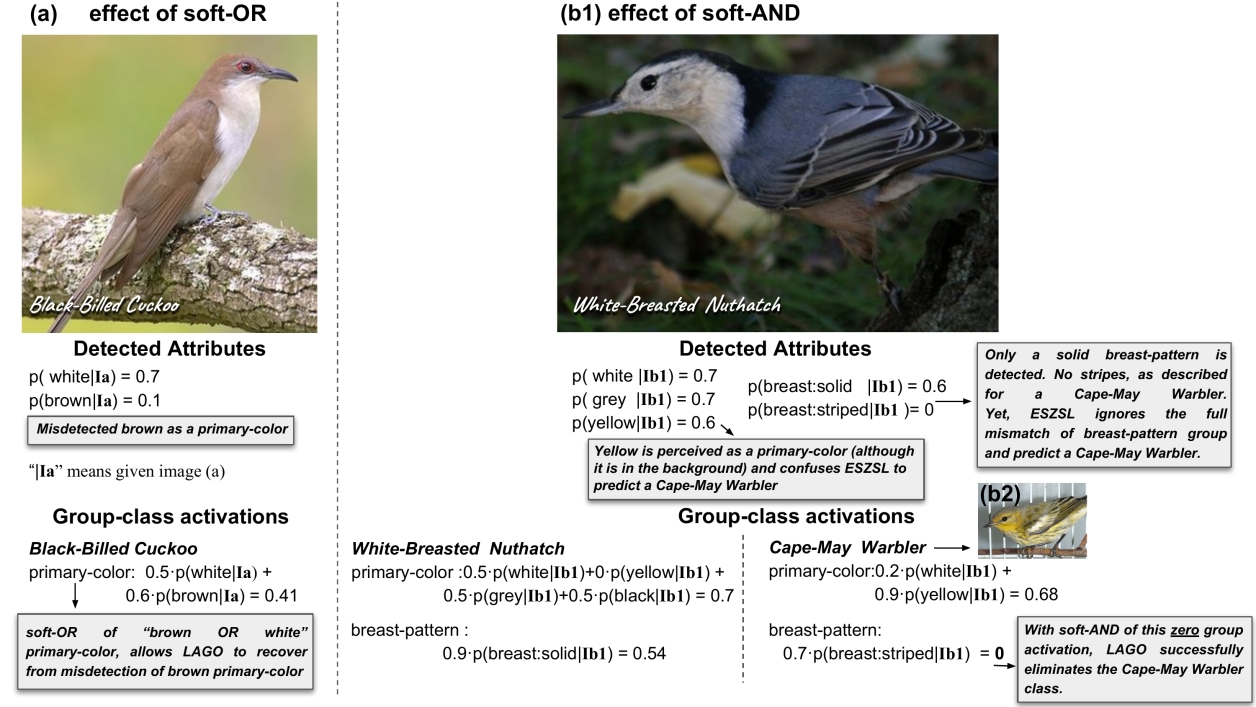
Figure 5: Qualitative examples. (a) LAGO correctly classifies a Black-billed Cuckoo, due to soft-OR of “brown or white” primary-color, although a detector misses its brown primary-color. (b1) LAGO correctly classifies a White-Breasted Nuthatch: The soft-intersection across groups prevents incorrect classification. ESZSL incorrectly classified Image (b1) as class of (b2), despite irrelevant attribute groups like its breast pattern (b2) A typical Cape-May Warbler. ESZSL mistakes (b1) image for this class

The effect of within-group disjunction (OR): Image 5a is correctly classified by LAGO as a Black-billed Cuckoo, even-though a detector misses its brown primary-color. In more detail, for this class, raters disagreed whether the primary-color is mostly brown ($p(brown|z)=0.6$) or white ($0.5$), because this property largely depends on the point-of view. Somewhat surprisingly, the primary color in this photo was detected to be mostly white (${p}(white|\mathbf{x})=0.7$), and hardly brown ($0.1$), perhaps because of a brown branch that interferes with segmenting out the bird. Missing the brown color hurts any classifier that requires both brown and white, like DAP. LAGO treats the detected primary color as a good match because it takes a soft OR relation over the two primary colors, hence avoids missing the right class.

The effect of group conjunction (AND): Image 5b.1 was correctly classified by LAGO as a White-Breasted Nuthatch, even-though a detector incorrectly detects a yellow primary color $({p}(yellow|\mathbf{x})=0.6)$ together with white and grey primary colors ($0.7$). As a comparison, the perceived yellow primary color confused ESZSL to mistake this image for a Cape-May Warbler, shown in image (b.2). Since ESZSL treats attributes as ”flat”, it does not use the fact that the breast pattern does not match a Warbler, and adheres to other attributes that produce a false positive detection of the Warbler. Yet, LAGO successfully avoids being confused by the yellow primary color, since the Nuthatch is expected to have a solid breast pattern, which is correctly detected ${p}(breast:solid|\mathbf{x})=0.6$. The Warbler is ranked lower because it is expected to have a striped breast pattern, which does not satisfy the AND condition because stripes are not detected $p(breast:striped|x)=0$.

4.4 ABLATION EXPERIMENTS

We carried empirical ablation experiments with the semantic hard-grouping of LAGO. Specifically, we tested three design decisions we made, as described above. (1) Uniform relates to taking a uniform prior for ${p}(a_{m})$, which is the average of the estimated ${p}(a_{m})$. “Per-attribute” relates to using the estimated ${p}(a_{m})$ directly. (2) Const relates to setting a constant value for the approximation of the complementary attribute ${p}(\tilde{a_{k}}|\mathbf{x})$. “DeMorgan” relates to approximating it from predictions of other attributes with De-Morgan’s rule. (3) Implicit relates to setting a zero weight ($\alpha=0$) for the loss term of the attribute supervision. I.e. attributes are learned implicitly, because only class-level super vision is given. “Explicit” related to setting a non-zero $\alpha$ respectively.

Table A.2 (in Supplementary) shows contributions of each combination of the design decisions to prediction accuracy, on the validation set of CUB and AWA2. The results are consistent for both CUB and AWA2. The most major effect is contributed for the uniform prior of ${p}(a_{m})$. All experiments that use the uniform prior yield better accuracy. We observe that taking a uniform prior also reduces variability due to the other approximations we take. Specifically, on CUB there is $\approx$ 4.5% best-to-worst gap with a uniform prior, vs $\approx$ 12.5% without ($\approx$ 11% vs $\approx$ 16% for AWA2 respectively). Next we observe that in the uniform case, approximating ${p}(\tilde{a_{k}}|\mathbf{x})$ by a constant, is superior to approximating it with De-Morgan’s rule, and similarly, reduces the impact of the variability of the implicit/explicit condition. Last, the contribution of attributes supervision condition mostly depends on selection of the previous two conditions.

5 DISCUSSION

Three interesting future research directions can be followed. First, since LAGO is probabilistic, one can plug measures for model uncertainty (Gal & Ghahramani, 2016), to improve model prediction and increase robustness to adversarial attacks. Second, descriptions of fine-grained categories often provide richer logical expressions to describe and differentiate classes. It will be interesting to study how LAGO may be extended to incorporate richer relations that could be explicitly discriminative (Vedantam et al., 2017). For example, Wikipedia describes White-Breasted-Nuthatch to make it distinct from other, commonly confused, Nuthatches by: “Three other, significantly smaller, nuthatches have ranges which overlap that of white-breasted, but none has white plumage completely surrounding the eye. ”.

Third, when people describe classes, they often use a handful of attributes instead of listing all values for the full set of attributes. The complementary attribute used in LAGO allows to model a “don’t-care” about a group, when no description is provided for a group. Such an approach could enable to recognize visual entities based on a handful and partial indication of semantic properties.

6 SUMMARY

We presented LAGO, a new probabilistic zero-shot-learning approach that can be trained end-to-end. LAGO approximates ${p}(class\!=\!z|image\!=\!\mathbf{x})$ by capturing natural soft and-or logical relations among groups of attributes, unlike most ZSL approaches that represent attributes as embedded in a “flat” space. LAGO learns the grouping structure from data, and can effectively incorporate prior domain knowledge about the grouping of attributes when available. We find that LAGO achieves new state-of-the-art result on CUB (Wah et al., 2011), AWA2 (Lampert et al., 2009), and is competitive on SUN (Patterson & Hays, 2012). Finally, LAGO reveals an interesting unified formulation over seemingly-unrelated ZSL approaches, DAP (Lampert et al., 2009) and ESZSL (Romera-Paredes & Torr, 2015).

SUPPLEMENTARY MATERIAL

A IMPLEMENTATION AND TRAINING DETAILS

The weights $W$ were initialized with orthogonal initialization (Saxe et al., 2014). The loss in Eq. (6) was optimized with Adam optimizer (Kingma & Ba, 2015). We used cross-validation to tune early stopping and hyper-parameters. When the learning rate is too high, the number of epochs for early-stopping varies largely with the weight seed. Therefore, we chose a learning rate that shows convergence within at least 40 epochs. Learning rate was searched in [3e-6, 1e-5, 3e-5, 1e-4, 3e-4]. From the top performing hyper-parameters, we chose the best one based on an average of additional 3 different seeds. Number-of-epochs for early stopping, was based on their average learning curve. For $\beta,\lambda$, L2 regularization params, we searched in [0, 1e-8, .., 1e-3].

For learning soft groups, we also tuned the learning rate of ${V}$ in [0.01, 0.1, 1], of $\zeta$ in [1, 3, 10], and when applicable, the number of groups $K$ in [1, 10, 20, 30, 40, 60], or semantic prior $\psi$ in [1e-5, .., 1e-2]. We tuned these hyper-params by first taking a coarse random search, and then further searching around the best performing values.

To comply with the mutual-exclusion approximation (2), if the group sum $\sum_{m\in G_{k}}{p}(a_{m}=T|z)$ is larger than 1, we normalize it to 1. We do not normalize if the sum is smaller than 1 in order to allow LAGO to account for the complementary case. We apply this normalization only for the LAGO-Semantic variants, where a prior knowledge about grouping is given.

After selecting hyper-parameters with cross-validation, models were retrained on both the training and the validation classes.

A.1 EVALUTATION METRIC

We follow Xian et al. (2017b) and use a class-balanced accuracy metric which averages correct predictions independently per-class before calculating the mean value:

$$acc_{\mathcal{Z}}=\frac{1}{|\mathcal{Z}|}\sum_{z=1}^{|\mathcal{Z}|}\frac{\text{\# of correct predictions in \,}z}{\text{\# of samples in \,}z}.$$ (A.7)

B LEARNED SOFT-GROUP ASSIGNMENTS ($\Gamma$)

We analyzed the structure of learned soft group assignments ($\Gamma_{m,k}={p}({m\in G_{k}})$) for LAGO-K-Soft, initialized by a uniform prior. We found two types of interesting structures:

First, we find that the learned $\Gamma$ tends to be sparse: with 2.5% non-zero values on SUN, 8.7% on AWA2 and 3.3% on CUB. As a result, the learned model has small groups, each with only a few attributes. Specifically, $\Gamma$ maps each attribute to only a single group on SUN (K=40 groups) and CUB (K=30), and to 2-3 groups on AWA2 (K=30 groups).

Second, we tested which attributes tend to be grouped together, and found that the model tends to group anti-correlated attributes. To do this, we first quantified for each pair of attributes, how often they tend to appear together in the data. Specifically, we estimated the occurrence pearson-correlation for each pair of attributes across samples (CUB, SUN) or classes (AWA2). Second, we computed the grouping similarity of two attributes as the inner product of their corresponding rows in Gamma, and considered an attribute pair to be grouped together if this product was positive (note that rows are very sparse). Using these two measures, we observed that the model tends to group anti-correlated attributes. This is consistent with human-based grouping, whose attribute are also often anti correlated (red foot, blue foot). In SUN, 45% of attribute-pairs that are grouped together were anti-correlated, compared to 23% of the full set of pairs. (AWA2 38% vs 5% baseline, CUB 16% vs 10% baseline). These differences were also highly significant statistically (Kolmogorov-Smirnov test p-value $<$ 3e-3)

C ROBUSTNESS TO NOISE

We tested LAGO-Semantic-Hard, LAGO-Singletons and ESZSL with various amount of salt & pepper noise (Figure A.1) injected to class-level description ${p}(a_{m}|z)$ of CUB. While LAGO-Semantic-Hard and ESZSL show a similar sensitivity to noise, LAGO-Singletons is more sensitive due to its all-AND structure.

Figure A.1: Robustness to salt & pepper noise. The relative accuracy on CUB of three models as a function of ration of injected noise to class-level description ${p}(a_{m}|z)$. Values are averages over 5 noise-seeds. LAGO-Semantic-Hard and ESZSL show a similar sensitivity to noise, while LAGO-Singletons is more sensitive due to its all-AND structure. The relative accuracy is calculated against each model own zero-noise baseline.

	CUB	AWA2	SUN
DAP	40.0	46.2	39.9
ALE	54.9	62.5	58.1
ESZSL	53.9	58.6	54.5
SYNC	55.6	46.6	56.3
SJE	53.9	61.9	53.7
DEVISE	52.0	59.7	56.5
ZHANG2018	48.7 - 57.1	58.3-70.5	57.8-61.7
LAGO-Singletons	54.5	63.7	57.3
LAGO-K-Soft	55.3	59.7	57.5
LAGO-Semantic-Hard	58.3	60.4	47.1
LAGO-Semantic-Soft	57.8	64.8	48.0
LAGO (cross-validation)	57.8	64.8	57.5

Table A.1: Test accuracy for all the variants of LAGO on three benchmark datasets, averaged over 5 random initializations of model weights. Standard-error-of-the-mean (S.E.M) is $\scriptstyle\sim$ 0.1% for the hard groups variants and $\scriptstyle\sim$ 0.4% for the soft-groups variants.

${p}(a_{m})$	$P(\tilde{a_{k}}|\mathbf{x})$	Attributes supervision	CUB	AWA2
Uniform	Const	Implicit	52.85	60.53
Uniform	Const	Explicit	52.17	60.17
Uniform	DeMorgan	Explicit	51.75	57.93
Uniform	DeMorgan	Implicit	48.41	49.54
Per-attribute	DeMorgan	Explicit	47.71	53.32
Per-attribute	Const	Explicit	42.68	52.05
Per-attribute	Const	Implicit	39.31	51.88
Per-attribute	DeMorgan	Implicit	35.3	37.21

Table A.2: Ablation experiments: Validation accuracy (in %) for CUB and AWA2, for combinations of model-design variants, with the semantic hard-grouping of LAGO. Results are given in descending order based on CUB. Uniform vs Per-attribute relates to taking a uniform prior for ${p}(a_{m})$. Const DeMorgan relates to setting a constant value for approximating the complementary attribute ${p}(\tilde{a_{k}}|\mathbf{x})$ vs an approximation derived by De-Morgan’s rule. Implicit vs Explicit relates to setting a zero weight ($\alpha=0$) for the loss term of the attribute supervision. Namely, attributes are learned implicitly, since only class-level super vision is given. The uniform prior on ${p}(a_{m})$ has the largest impact, second is the usage of a constant value for ${p}(\tilde{a_{k}}|\mathbf{x})$, and the last relates to nulling the attribute supervision loss. See details on Section 4.4

D DETAILED DERIVATION

D.1 ${p}(a_{m}|g_{k,z}\!\!=\!\!T)$ EQUALS ${p}(a_{m}|Z\!\!=\!\!z)$

Here we explain why Eq. (A.8) below is true.

$${p}(a_{m}|g_{k,z}\!\!=\!\!T)={p}(a_{m}|Z\!\!=\!\!z),$$ (A.8)

It is based on the definition of $g_{k,z}$: $g_{k,z}$ is the classifier of $z$ based on $\mathbf{a}_{k}$. Therefore $p(g_{k,z}|\mathbf{a}_{k})\!\!=\!\!p(z|\mathbf{a}_{k})$, and by marginalization we get: (*) ${p}(g_{k,z}\!=\!T,a_{m})\!\!=\!\!{p}(z,a_{m})$, (**) ${p}(g_{k,z}\!=\!T)\!\!=\!\!{p}(Z\!=\!z)$. Next, using conditional probability chain rule on (*), yields

$${p}(a_{m}|g_{k,z}\!=\!T){p}(g_{k,z}\!=\!T)={p}(a_{m}|Z=z){p}(Z=z)\quad.$$ (A.9)

Then, (**) transforms (A.9) to the required equality:

$${p}(a_{m}|g_{k,z}\!=\!T)={p}(a_{m}|Z=z)\quad.$$ (A.10)

Intuitively, the right side of (A.10), is the probability of observing $a_{m}$ for a class $z$, like ${p}(stripes|zebra)$. This is the same probability of observing the attribute given the class while focusing on its respective group, namely ${p}(a_{m}\!=\!T|g_{k,z}\!=\!T)\!=\!{p}(stripes|\textit{focus on zebra pattern})$.

D.2 DERIVATION OF GROUP CONJUNCTION:

This derivation is same as in DAP (Lampert 2009), except we apply it at the group level rather than the attribute level. We denote ${g_{1,z}\dots g_{K,z}}$ by $\mathbf{g}_{z}$ and approximate the following combinatorially large sum:

$${p}(Z\!=\!z|\mathbf{x})\!=\!\sum_{\mathbf{g}_{z}\in\{T,F\}^{K}}{p}(Z\!=\!z|\mathbf{g}_{z}){p}(\mathbf{g}_{z}|\mathbf{x})\quad.$$ (A.11)

First, using Bayes (A.11) becomes

$$\sum_{\mathbf{g}_{z}\in\{T,F\}^{K}}\frac{{p}(\mathbf{g}_{z}|Z\!=\!z){p}(Z\!=\!z)}{{p}(\mathbf{g}_{z})}{p}(\mathbf{g}_{z}|\mathbf{x})$$ (A.12)

Second, we approximate ${p}(\mathbf{g}_{z}|Z\!=\!z)$ to be

$${p}(\mathbf{g}_{z}|Z\!=\!z)=\begin{cases}1,&\text{if}\ g_{1,z}\!=\!T\dots g_{K,z}\!=\!T\\ 0,&\text{otherwise}\end{cases}$$ (A.13)

which transforms (A.12) to

$${p}(Z\!=\!z|\mathbf{x})\!\approx{p}(Z\!=\!z)\frac{{p}(g_{1,z}\!=\!T\dots g_{K,z}\!=\!T|\mathbf{x})}{{p}(g_{1,z}\!=\!T\dots g_{K,z}\!=\!T)}$$ (A.14)

Third, we approximate the numerator of (A.14) with the assumption of conditional independence of groups given an image (by observing an image we can judge each group independently),

$${p}(g_{1,z}\!=\!T\dots g_{K,z}\!=\!T|\mathbf{x})\approx\prod\limits_{k=1}^{K}{p}(g_{k,z}\!=\!T|\mathbf{x})$$ (A.15)

Fourth, we approximate the denominator of (A.14) to its factored form ${p}(g_{1,z}\!=\!T\dots g_{K,z}\!=\!T)\approx\prod\limits_{k=1}^{K}{{p}(g_{k,z}\!=\!T)}$, and with (A.15) we arrive at:

$${p}(Z\!=\!z|\mathbf{x})\approx{p}(Z\!=\!z)\prod\limits_{k=1}^{K}\frac{{p}(g_{k,z}\!=\!T|\mathbf{x})}{{p}(g_{k,z}\!=\!T)}\quad.$$ (A.16)

D.3 A DERIVATION OF SOFT GROUP MODEL

Here we adapt LAGO to account for soft group-assignments for attributes, by extending the within-group part of the model. We start with partitioning ${p}(g_{k,z}\!=\!T|\mathbf{x})$ to a union (OR) of its contributions, repeated below for convenience,

$${p}(g_{k,z}|\mathbf{x})=\\ {p}(g_{k,z},\mathop{\mathbin{\scalebox{1.5}{$\cup$}}}\limits_{m\in G_{k}}a_{m}=T|\mathbf{x})+{p}(g_{k,z},\tilde{a_{k}}=T|\mathbf{x}),$$ (A.17)

and instead, treat the attribute-to-group assignment ${(m\in G_{k})}$, as a probabilistic assignment, yielding:

$${p}(g_{k,z}|\mathbf{x})=\\ {p}(g_{k,z},\mathop{\mathbin{\scalebox{1.5}{$\cup$}}}\limits_{m=1}^{|\mathcal{A}|}({m\in G_{k}},a_{m}=T|\mathbf{x}))+{p}(g_{k,z},\tilde{a_{k}}=T|\mathbf{x}),$$ (A.18)

Note that the attribute-to-group assignment $(m\in G_{k})$ is independent of the current given image $\mathbf{x}$, class $z$ or the True / False occurrence of an attribute $a_{m}$. Repeating the mutual exclusion approximation (2) yields,

$${p}(g_{k,z}|\mathbf{x})\approx\sum_{m=1}^{|\mathcal{A}|}{p}(g_{k,z},{m\in G_{k}},a_{m}=T|\mathbf{x}).$$ (A.19)

Using the independence of $({m\in G_{k}})$, yields

$${p}(g_{k,z}|\mathbf{x})\approx\sum_{m=1}^{|\mathcal{A}|}{p}({m\in G_{k}}){p}(g_{k,z},a_{m}=T|\mathbf{x}).$$ (A.20)

Defining $\Gamma_{m,k}={p}({m\in G_{k}})$, yields:

$${p}(g_{k,z}|\mathbf{x})\approx\sum_{m=1}^{|\mathcal{A}|}\Gamma_{m,k}{p}(g_{k,z},a_{m}=T|\mathbf{x}).$$ (A.21)

As in section 3, using the Markov chain property $\mathcal{X}\rightarrow\mathcal{A}\rightarrow\mathcal{G}$ and ${p}(g_{k,z}=T|a_{m})=\frac{{p}(a_{m}|z){p}(g_{k,z}=T)}{{p}(a_{m})}$ results with Eq. (5), repeated below:

$${p}(g_{k,z}=T|\mathbf{x}){}\approx\\ {p}(g_{k,z}=T)\sum_{m=1}^{|\mathcal{A}|}\Gamma_{m,k}\frac{{p}(a_{m}=T|z)}{{p}(a_{m}=T)}{p}(a_{m}=T|\mathbf{x})$$ (A.22)

D.3.1 APPROXIMATING THE COMPLEMENTARY TERM

With soft groups, the complementary term is defined as

$$\tilde{a_{k}}=\Big{(}\mathop{\mathbin{\scalebox{1.5}{$\cup$}}}\limits_{m=1}^{|\mathcal{A}|}({m\in G_{k}},a_{m}=T|\mathbf{x}))\Big{)}^{c}$$ (A.23)

To approximate ${p}(\tilde{a_{k}}=T|z)$ we can use De-Morgan’s rule over a factored joint conditional probability of group-attributes. I.e.

$${p}(\tilde{a_{k}}=T|z)\approx\prod_{m=1}^{|\mathcal{A}|}(1-{p}({m\in G_{k}},a_{m}=T|z))=\\ \prod_{m=1}^{|\mathcal{A}|}(1-\Gamma_{m,k}{p}(a_{m}=T|z)),$$ (A.24)

where the latter term is derived by the independence of $({m\in G_{k}})$

D.4 DAP, ESZSL AS SPECIAL CASES OF LAGO

Two extreme cases of LAGO are of special interest: having each attribute in its own singleton group ($K=|A|$), and having one big group over all attributes ($K=1$).

Consider first assigning each single attribute $a_{m}$ to its own singleton group ($K=|A|$ and $m=k$). We remind that we defined $G_{k}^{\prime}=G_{k}\mathop{\mathbin{\scalebox{1.5}{$\cup$}}}\tilde{a_{k}}$. Therefore, $G_{k}^{\prime}$ has only two attributes $\{a_{m},\tilde{a_{k}}\}$, which turns the sum in Eq. (4), to a sum over those elements:

$${p}(z|\mathbf{x}){}=\,\,\,\,{p}(z)\prod\limits_{k=1}^{K}\Big{[}\frac{{p}(a_{m}\!=\!T|z)}{{p}(a_{m}\!=\!T)}{p}(a_{m}\!\!=\!\!T|\mathbf{x})+\\ \!\!\frac{{p}(\tilde{a_{k}}\!=\!T|z)}{{p}(\tilde{a_{k}}\!=\!T)}{p}(\tilde{a_{k}}\!\!=\!\!T|\mathbf{x})\Big{]}.$$ (A.25)

In a singleton group, the complementary attribute $\tilde{a_{k}}$ becomes $\tilde{a_{k}}=a_{m}^{c}$, and therefore
$\tilde{a_{k}}\!=\!T\Leftrightarrow a_{m}\!=\!F$. This transforms (A.25) to:

$${p}(z|\mathbf{x}){}=\,\,\,\,{p}(z)\prod\limits_{m=1}^{|A|}\Big{[}\frac{{p}(a_{m}\!\!=\!\!T|z)}{{p}(a_{m}\!\!=\!\!T)}{p}(a_{m}\!\!=\!\!T|\mathbf{x})+\\ \frac{{p}(a_{m}\!\!=\!\!F|z)}{{p}(a_{m}\!\!=\!\!F)}{p}(a_{m}\!\!=\!\!F|\mathbf{x})\Big{]}\quad.$$ (A.26)

This formulation is closely related to DAP (Lampert et al., 2009), where the expert annotation ${p}(a_{m}\!\!=\!\!T|z)$ is thresholded to $\{0,1\}$ using the mean of the matrix ${U}$ as a threshold, and denoted by $a^{z}_{m}$. Applying a similar threshold to Eq. (A.26) yields

$${p}(z|\mathbf{x}){}={p}(z)\prod\limits_{m=1}^{|A|}\Big{[}\frac{a^{z}_{m}}{{p}(a_{m}\!\!=\!\!T)}{p}(a_{m}\!\!=\!\!T|\mathbf{x})+\\ \frac{(1-a^{z}_{m})}{{p}(a_{m}\!\!=\!\!F)}{p}(a_{m}\!\!=\!\!F|\mathbf{x})\Big{]}$$ (A.27)

Reducing Eq. (A.27), by taking only the cases where it is non-zero for its two parts, gives the posterior of DAP

$${p}(z|\mathbf{x}){}=\\ {p}(z)\prod\limits_{m=1}^{|A|}\frac{{p}(a_{m}\!\!=\!\!a^{z}_{m}|\mathbf{x})}{{p}(a_{m}\!\!=\!\!a^{z}_{m})}\quad.$$ (A.28)

This derivation reveals that in the extreme case of $K=|A|$ singleton groups, LAGO becomes equivalent to a soft relaxation of DAP.

At the second extreme, consider the case where all attributes are assigned to a single group, $K\!=\!1$. Taking a uniform prior for ${p}(z)$ and ${p}(a_{m})$, and writing ${p}(a_{m}=T|\mathbf{x})$ using the network model $\sigma(\mathbf{x}^{\top}W)$, transforms Eq. (4) to:

$${p}(z|\mathbf{x})\propto\sum\limits_{m=1}^{|A|}\sigma(\mathbf{x}^{\top}W){p}(a_{m}=T|z).$$ (A.29)

This can be viewed as a 2-layer architecture: First map image features to a representation in the attribute dimension, then map it to class scores by an inner product with the supervised entries of attributes-to-classes ${U}_{m,z}={p}(a_{m}=T|z)$. This formulation resembles ESZSL, which uses a closely related 2-layer architecture: $Score(z|\mathbf{x})=\mathbf{x}^{\top}WU$, where $W$ first maps image features to a representation in the same attribute dimension, and then map it to class scores, with an inner product by the same attributes-to-classes entries ${U}_{m,z}={p}(a_{m}=T|z)$. LAGO differs from ESZSL in two main ways: (1) The attribute-layer in LAGO uses a sigmoid-activation, while ESZSL uses a linear activation. (2) LAGO uses a cross-entropy loss, while ESZSL uses mean-squared-error. This allows ESZSL to have a closed-form solution where reaching the optimum is guaranteed.

This derivation reveals that at the extreme case of $K=1$, LAGO can be viewed as a non-linear variant that is closely related to ESZSL.

References

- Akata et al. (2015) Z. Akata, S. Reed, D. Walter, Honglak Lee, and B. Schiele. Evaluation of output embeddings for fine-grained image classification. In CVPR, 2015.
- Akata et al. (2016) Z. Akata, F. Perronnin, Z. Harchaoui, and C. Schmid. Label-embedding for image classification. IEEE Transactions on Pattern Analysis and Machine Intelligence (TPAMI), 2016.
- Al-Halah & Stiefelhagen (2015) Z. Al-Halah and R. Stiefelhagen. How to transfer? zero-shot object recognition via hierarchical transfer of semantic attributes. In WACV, 2015.
- Arora et al. (2018) G. Arora, V-K. Verma, A. Mishra, and P. Rai. Generalized zero-shot learning via synthesized examples. In CVPR, 2018.
- Bach et al. (2017) S. Bach, M. Broecheler, B. Huang, and L. Getoor. Hinge-loss markov random fields and probabilistic soft logic. Journal of Machine Learning Research, 2017.
- Berg et al. (2010) T. Berg, A.C. Berg, and J. Shih. Automatic attribute discovery and characterization from noisy web data. In ECCV. Springer, 2010.
- Changpinyo et al. (2016) S. Changpinyo, W. L. Chao, B. Gong, and F. Sha. Synthesized classifiers for zero-shot learning. In CVPR, 2016.
- Elhoseiny et al. (2013) M. Elhoseiny, B. Saleh, and A. Elgammal. Write a classifier: Zero-shot learning using purely textual descriptions. In ICCV, 2013.
- Farhadi et al. (2009) A. Farhadi, I. Endres, D. Hoiem, and D. Forsyth. Describing objects by their attributes. In CVPR. IEEE, 2009.
- Ferrari & Zisserman (2008) V. Ferrari and A. Zisserman. Learning visual attributes. In NIPS, pp. 433–440, 2008.
- Frome et al. (2013) A. Frome, G. Corrado, J. Shlens, S. Bengio, J. Dean, M. Ranzato, and T. Mikolov. Devise: A deep visual-semantic embedding model. In NIPS, 2013.
- Fu et al. (2017) Y. Fu, T. Xiang, Y-G Jiang, X. Xue, L. Sigal, and S. Gong. Recent advances in zero-shot recognition. arXiv preprint arXiv:1710.04837, 2017.
- Gal & Ghahramani (2016) Y. Gal and Z. Ghahramani. Dropout as a bayesian approximation: Representing model uncertainty in deep learning. In ICML, 2016.
- Guo et al. (2018) Y. Guo, G. Ding, J. Han, and S. Tang. Zero-shot learning with attribute selection. In AAAI, 2018.
- Jayaraman et al. (2014) D. Jayaraman, F. Sha, and K. Grauman. Decorrelating semantic visual attributes by resisting the urge to share. In CVPR, CVPR ’14, 2014.
- Jiang et al. (2017) H. Jiang, R. Wang, S. Shan, Y. Yang, and X. Chen. Learning discriminative latent attributes for zero-shot classification. In ICCV, 2017.
- Kemp et al. (2006) C. Kemp, JB. Tenenbaum, T.L. Griffiths, T. Yamada, and N. Ueda. Learning systems of concepts with an infinite relational model. In AAAI, volume 1, 2006.
- Kimmig et al. (2012) A. Kimmig, S. Bach, M. Broecheler, B. Huang, and L. Getoor. A short introduction to probabilistic soft logic. In NIPS Workshop on Probabilistic Programming, 2012.
- Kingma & Ba (2015) D.P. Kingma and J. Ba. Adam: A method for stochastic optimization. In ICLR, 2015.
- Lampert (2011) C.H. Lampert. Semantic attributes for object categorization (slides). ist.ac.at/chl/talks/lampert-vrml2011b.pdf, 2011.
- Lampert et al. (2009) C.H. Lampert, H. Nickisch, and S. Harmeling. Learning to detect unseen object classes by between-class attribute transfer. In CVPR. IEEE, 2009.
- Lampert et al. (2014) C.H. Lampert, H. Nickisch, and S. Harmeling. Attribute-based classification for zero-shot visual object categorization. IEEE Transactions on Pattern Analysis and Machine Intelligence (TPAMI), 36(3), 2014.
- Li et al. (2017) Y. Li, D. Wang, H. Hu, Y. Lin, and Y. Zhuang. Zero-shot recognition using dual visual-semantic mapping paths. In CVPR, 2017.
- Mishra et al. (2018) A. Mishra, M. Reddy, A. Mittal, and H. A. Murthy. A generative model for zero shot learning using conditional variational autoencoders. In WACV, 2018.
- Morgado & Vasconcelos (2017) P. Morgado and N. Vasconcelos. Semantically consistent regularization for zero-shot recognition. In CVPR. IEEE, 2017.
- Osherson et al. (1991) D. N. Osherson, J. Stern, O. Wilkie, M. Stob, and E. Smith. Default probability. Cognitive Science, 15(2), 1991.
- Palatucci et al. (2009) M. Palatucci, D. Pomerleau, G. E Hinton, and T.M. Mitchell. Zero-shot learning with semantic output codes. In NIPS, 2009.
- Park & Zhu (2015) S. Park and S. C. Zhu. Attributed grammars for joint estimation of human attributes, part and pose. In ICCV, 2015.
- Park et al. (2017) S. Park, X. Nie, and S. C. Zhu. Attribute and-or grammar for joint parsing of human pose, parts and attributes. IEEE Transactions on Pattern Analysis and Machine Intelligence (TPAMI), 2017.
- Patterson & Hays (2012) G. Patterson and J. Hays. Sun attribute database: Discovering, annotating, and recognizing scene attributes. In CVPR, 2012.
- Richardson & Domingos (2006) M. Richardson and P. Domingos. Markov logic networks. Machine Learning, 62(1), 2006.
- Rohrbach et al. (2011) M. Rohrbach, M. Stark, and B. Schiele. Evaluating knowledge transfer and zero-shot learning in a large-scale setting. In CVPR, 2011.
- Romera-Paredes & Torr (2015) B. Romera-Paredes and P. Torr. An embarrassingly simple approach to zero-shot learning. In ICML, 2015.
- Saxe et al. (2014) A.M. Saxe, J. L McClelland, and S. Ganguli. Exact solutions to the nonlinear dynamics of learning in deep linear neural networks. ICLR, 2014.
- Socher et al. (2013) R. Socher, M. Ganjoo, C.D. Manning, and A. Ng. Zero-shot learning through cross-modal transfer. In NIPS, 2013.
- Tsai et al. (2017a) Y-H. Tsai, L-K. Huang, and R. Salakhutdinov. Learning robust visual-semantic embeddings. In ICCV, 2017a.
- Tsai et al. (2017b) Y-H H. Tsai, L-K Huang, and R. Salakhutdinov. Learning robust visual-semantic embeddings. In ICCV, 2017b.
- Vedantam et al. (2017) R. Vedantam, S. Bengio, K. Murphy, D. Parikh, and G. Chechik. Context-aware captions from context-agnostic supervision. In CVPR, 2017.
- Wah et al. (2011) C. Wah, S. Branson, P. Welinder, P. Perona, and S. Belongie. The Caltech-UCSD Birds-200-2011 Dataset. Technical Report CNS-TR-2011-001, California Institute of Technology, 2011.
- Wang & Ji (2013) X. Wang and Q. Ji. A unified probabilistic approach modeling relationships between attributes and objects. In ICCV, 2013.
- Xian et al. (2017a) Y. Xian, C.H. Lampert, B. Schiele, and Z. Akata. Zero-shot learning - A comprehensive evaluation of the good, the bad and the ugly. arXiv preprint arXiv:1707.00600, 2017a.
- Xian et al. (2017b) Y. Xian, B. Schiele, and Z. Akata. Zero-shot learning - the good, the bad and the ugly. In CVPR, 2017b.
- Xian et al. (2018) Y. Xian, T. Lorenz, B. Schiele, and Z. Akata. Feature generating networks for zero-shot learning. In CVPR, 2018.
- Xu et al. (2017) X. Xu, F. Shen, Y. Yang, D. Zhang, H. T. Shen, and J. Song. Matrix tri-factorization with manifold regularizations for zero-shot learning. In CVPR, 2017.
- Ye & Guo (2017) M. Ye and Y. Guo. Zero-shot classification with discriminative semantic representation learning. In CVPR, 2017.
- Zhang & Koniusz (2018) Hongguang Zhang and Piotr Koniusz. Zero-shot kernel learning. In CVPR, 2018.
- Zhang et al. (2017) L. Zhang, T. Xiang, and S. Gong. Learning a deep embedding model for zero-shot learning. In CVPR, 2017.
- Zhu & Mumford (2006) S-C Zhu and D. Mumford. A stochastic grammar of images. Found. Trends. Comput. Graph. Vis., 2(4), 2006.