Scalable Multi-Class Bayesian Support Vector Machines for Structured and Unstructured Data

Abstract

We introduce a new Bayesian multi-class support vector machine by formulating a pseudo-likelihood for a multi-class hinge loss in the form of a location-scale mixture of Gaussians. We derive a variational-inference-based training objective for gradient-based learning. Additionally, we employ an inducing point approximation which scales inference to large data sets. Furthermore, we develop hybrid Bayesian neural networks that combine standard deep learning components with the proposed model to enable learning for unstructured data. We provide empirical evidence that our model outperforms the competitor methods with respect to both training time and accuracy in classification experiments on 68 structured and two unstructured data sets. Finally, we highlight the key capability of our model in yielding prediction uncertainty for classification by demonstrating its effectiveness in the tasks of large-scale active learning and detection of adversarial images.

1 Introduction

Maximum margin classifiers like support vector machines (SVMs) [7] are arguably one of the most popular classification models. Cortes and Vapnik [7] famously introduced the linear binary SVM as a novel concept which was later extended by Boser et al. [4] using the kernel trick [13] to the non-linear kernel SVM. Numerous approaches exist to extend binary SVMs to multi-class classification tasks [9]. One classical approach is to combine multiple binary classifiers using the one-vs-one or one-vs-rest schemes. Alternate approaches involve defining a multi-class hinge loss [9], including the seminal work by Crammer and Singer [8], which learn a single model.

One key aspect of prediction models which is often overlooked by traditional approaches, including SVMs, is the representation and propagation of uncertainty. In general, decision makers are not solely interested in predictions but also in the confidence about the predictions. An action might only be taken in the case when the model in consideration is certain about its prediction. Bayesian formalism provides a principled way to obtain these uncertainties. Bayesian methods handle all kinds of uncertainties in a model, be it in inference of parameters or for obtaining the predictions. These methods are known to be effective for online classification [21], active learning [29], global optimization of expensive black-box functions [14], automated machine learning [32, 36], and as recently noted, even in machine learning security [30].

Therefore, it is natural to look for a Bayesian extension of SVM classifiers. Polson et al. [26] derive a pseudo-likelihood which, when being maximized, is the Bayesian equivalent to training a binary linear SVM. Henao et al. [11] extend this work to a non-linear version by modeling the decision function with a Gaussian process. Furthermore, they propose the use of a sparse approximation of the Gaussian process [31] to scale the Bayesian SVM. More recently, the use of a variational sparse approximation [33] has been proposed by Wenzel et al. [34].

The contributions in this work are threefold. We derive a pseudo-likelihood for a multi-class hinge loss and propose a multi-class Bayesian SVM. We provide a scalable learning scheme based on variational inference [3, 33, 12] to train the multi-class Bayesian SVM. Additionally, we propose a hybrid Bayesian neural network which combines deep learning components such as convolutional layers with the Bayesian SVM. This allows to jointly learn the feature extractors as well as the classifier design such that it can be applied both on structured and unstructured data. We compare the proposed multi-class SVM on 68 structured data sets to a state-of-the-art binary Bayesian SVM with the one-vs-rest approach and the scalable variational Gaussian process [12]. On average, the multi-class SVM provides better prediction performance and needs up to an order of magnitude less training time in comparison to the competitor methods. The proposed hybrid Bayesian neural network is compared on the image classification data sets MNIST [20] and CIFAR-10 [18] to a standard (non-Bayesian) neural network. We show that we achieve similar performance, however, require increased training time. Finally, we demonstrate the effectiveness of uncertainties in experiments on active learning and adversarial detection.

2 Related Work

Polson et al. [26] make a key observation and reformulate the hinge loss in the linear SVM training objective to a location-scale mixture of Gaussians. They derive a pseudo-likelihood by introducing local latent variables for each data point and marginalize them out. A non-linear version of this setup is considered by Henao et al. [11] where the linear decision function is modeled as a Gaussian process. They approximate the resulting joint posterior using Markov chain Monte Carlo (MCMC) or expectation conditional maximization (ECM). Furthermore, they scale the inference using the fully independent training conditional approximation (FITC) [31]. The basic assumption behind FITC is that the function values are conditionally independent given the set of inducing points. Then, training the Gaussian process is no longer cubically dependent on the number of training instances. Moreover, the number of inducing points can be freely chosen. Luts and Ormerod [23] extend the work of Polson et al. [26] by applying a mean field variational approach to it. Most recently, Wenzel et al. [34] propose an alternate variational objective and use coordinate ascent to maximize it. They demonstrate improved performance over a classical SVM, competitor Bayesian SVM approaches, and Gaussian process-based classifiers.

Another important related topic is Gaussian process-based classifiers [35]. As opposed to Bayesian SVMs, these classifiers directly use a decision function with a probit or logit link function [27]. Gaussian process classifiers often perform similar to non-linear SVMs [19] and hence, are preferred by some practitioners due to added advantages like uncertainty representation and automatic hyperparameter determination. In this aspect the closest work to our approach is scalable variational Gaussian processes [12]. Like our proposed model, it tackles multi-class classification with a single model and uses variational inference with inducing point approximation to scale to large data sets.

3 Bayesian Support Vector Machines

This section details the proposed multi-class Bayesian SVM. We begin with a discussion of a Bayesian formulation of a binary SVM and follow it with the multi-class case.

3.1 Binary SVM

SVM

For a binary classification task, support vector machines seek to learn a decision boundary with maximum margin, i.e. the separation between the decision boundary and the instances of the two classes. We represent the labeled data for a binary classification task with $N$ observations and $M$-dimensional representation as $D=\{\mathbf{x}_{n},y_{n}\}_{n=1}^{N}$, where $\mathbf{x}_{n}\in\mathbb{R}^{M}$ and $y_{n}\in\left\{-1,1\right\}$ represent predictors and labels, respectively. Training a binary SVM involves learning a decision function $f:\mathbb{R}^{M}\rightarrow\mathbb{R}$ that minimizes the regularized hinge loss,

$$\mathcal{L}\left(D,f,\gamma\right)=\sum_{n=1}^{N}\max\left\{1-y_{n}f\left(\mathbf{x}_{n}\right),0\right\}+\gamma R\left(f\right)\enspace.$$ (1)

The regularizer $R$ punishes the choice of more complex functions for $f$, and $\gamma$ is a hyperparameter that controls the impact of this regularization. A linear SVM uses a linear decision function $f(\mathbf{x}_{n})=\boldsymbol{\theta}^{T}\mathbf{x}_{n}$. Non-linear decision functions are traditionally obtained by applying the kernel trick [13].

Bayesian Binary SVM

For the linear case, Polson et al. [26] show that minimizing Equation (1) is equivalent to estimating the mode of a pseudo-posterior (maximum a posteriori estimate)

$$p\left(f|D\right)\propto\exp\left(-\mathcal{L}\left(D,f,\gamma\right)\right)\propto\prod_{n=1}^{N}L\left(y_{n}|\mathbf{x}_{n},f\right)p\left(f\right),$$ (2)

derived for a particular choice of pseudo-likelihood factors $L$, defined by location-scale mixtures of Gaussians. This is achieved by introducing local latent variables $\lambda_{n}$ such that for each instance,

$$L\left(y_{n}|\mathbf{x}_{n},f\right)=\int_{0}^{\infty}\frac{1}{\sqrt{2\pi\lambda_{n}}}\exp\left(-\frac{1}{2}\frac{\left(1+\lambda_{n}-y_{n}f\left(\mathbf{x}_{n}\right)\right)^{2}}{\lambda_{n}}\right)\mathrm{d}\lambda_{n}\enspace.$$ (3)

In their formulations, Polson et al. [26] and Henao et al. [11] consider $\gamma$ as a model parameter and accordingly develop inference schemes. Similar to Wenzel et al. [34], we treat $\gamma$ as a hyperparameter and drop it from the expressions of prior and posterior for notational convenience. Henao et al. [11] extend this framework to enable learning of a non-linear decision function $f$. Both Henao et al. [11] and Wenzel et al. [34] consider models where $f(x)$ is sampled from a zero-mean Gaussian process i.e. $\mathbf{f}\sim\mathcal{N}(0,K_{NN})$, where $\mathbf{f}=[f(\mathbf{x}_{1}),\dots,f(\mathbf{x}_{n})]$ is a vector of decision function evaluations and $K_{NN}$ is the covariance function evaluated at data points. While Henao et al. [11] consider MCMC and ECM to learn the conditional posterior $p(\mathbf{f}|D,\boldsymbol{\lambda})$, Wenzel et al. [34] learn an approximate posterior $q(\mathbf{f},\boldsymbol{\lambda})$ with variational inference.

3.2 Bayesian Multi-Class SVM

A multi-class classification task involves $N$ observations with integral labels $Y=\left\{1,\dots,C\right\}$. A classifier for this task can be modeled as a combination of a decision function $f:\mathbb{R}^{M}\rightarrow\mathbb{R}^{C}$ and a decision rule to compute the class labels, $\hat{y}\left(\mathbf{x}_{n}\right)=\operatorname*{arg\,max}_{t\in Y}f_{t}\left(\mathbf{x}_{n}\right)$. Crammer and Singer [8] propose to minimize the following objective function for learning the decision function $f$:

$$\mathcal{L}\left(D,f,\gamma\right)=\sum_{n=1}^{N}\max\left\{1+\max_{t\neq y_{n},t\in Y}f_{t}\left(\mathbf{x}_{n}\right)-f_{y_{n}}\left(\mathbf{x}_{n}\right),\ 0\right\}+\gamma R\left(f\right)\enspace,$$ (4)

where again $\gamma$ is a hyperparameter controlling the impact of the regularizer $R$. With the prior associated to $\gamma R\left(f\right)$, maximizing the log of Equation (2) corresponds to minimizing Equation (4) with respect to the parameters of $f$. This correspondence requires the following equation to hold true for the data-dependent factors of the pseudo-likelihood,

$$\prod_{n=1}^{N}L\left(y_{n}\ |\ \mathbf{x}_{n},f\right)=\exp\left(-2\sum_{n=1}^{N}\max\left\{1+\max_{t\neq y_{n},t\in Y}f_{t}\left(\mathbf{x}_{n}\right)-f_{y_{n}}\left(\mathbf{x}_{n}\right),\ 0\right\}\right)\enspace.$$ (5)

Analogously to Polson et al. [26], we show that $L\left(y_{n}\ |\ \mathbf{x}_{n},f\right)$ admits a location-scale mixture of Gaussians by introducing local latent variables $\boldsymbol{\lambda}=[\lambda_{1},\dots,\lambda_{n}]$. This requires the lemma established by Andrews and Mallows [2].

Lemma 1.

For any $a,b>0$,

$$\int_{0}^{\infty}\frac{a}{\sqrt{2\pi\lambda}}e^{-\frac{1}{2}\left(a^{2}\lambda+b^{2}\lambda^{-1}\right)}\mathrm{d}\lambda=e^{-\left|ab\right|}\enspace.$$ (6)

Theorem 1.

The pseudo-likelihood contribution from an observation $y_{n}$ can be expressed as

$$L\left(y_{n}\ |\ \mathbf{x}_{n},f\right)=\int_{0}^{\infty}\frac{1}{\sqrt{2\pi\lambda_{n}}}\exp\left(-\frac{1}{2}\frac{\left(1+\lambda_{n}+\max_{t\neq y_{n},t\in Y}f_{t}\left(\mathbf{x}_{n}\right)-f_{y_{n}}\left(\mathbf{x}_{n}\right)\right)^{2}}{\lambda_{n}}\right)\mathrm{d}\lambda_{n}$$ (7)

Proof.

Applying Lemma 1 while substituting $a=1$ and $b=1+\max_{t\neq y_{n},t\in Y}f_{t}\left(\mathbf{x}_{n}\right)-f_{y_{n}}\left(\mathbf{x}_{n}\right)$, multiplying through by $e^{-b}$, and using the identity $\max\left\{b,0\right\}=\frac{1}{2}\left(\left|b\right|+b\right)$, we get,

$$\int_{0}^{\infty}\frac{1}{\sqrt{2\pi\lambda_{n}}}\exp\left(-\frac{1}{2}\frac{\left(b+\lambda_{n}\right)^{2}}{\lambda_{n}}\right)\mathrm{d}\lambda_{n}=e^{-2\max\left\{b,0\right\}}\enspace.$$ (8)

∎

Inference

We complete the model formulation by assuming that $f_{j}(\mathbf{x})$ is drawn from a Gaussian process for each class, $j$, i.e. $\mathbf{f}_{j}\sim\mathcal{N}(0,K_{NN})$ and $\boldsymbol{\lambda}\sim\mathbbm{1}_{[0,\infty)}(\boldsymbol{\lambda})$. Inference in our model amounts to learning the joint posterior $p(\mathbf{f},\boldsymbol{\lambda}|D)$, where $\mathbf{f}=[\mathbf{f}_{1},\dots,\mathbf{f}_{C}]$. However, computing the exact posterior is intractable and hence various schemes can be adopted to approximate it. In our approach we use variational inference combined with an inducing point approximation for scalable learning.

3.3 Scalable Variational Inference with Inducing Points

In variational inference, the exact posterior over the set of model parameters $\boldsymbol{\theta}$ is approximated by a variational distribution $q$. The parameters of $q$ are updated with the aim to reduce the dissimilarity between the exact and approximate posteriors, as measured by the Kullback-Leibler divergence. This is equivalent to maximizing the evidence lower bound (ELBO)  [15] with respect to parameters of $q$.

$$\operatorname{ELBO}=\mathbb{E}_{q(\boldsymbol{\theta})}\left[\log p\left(\mathbf{y}|\boldsymbol{\theta}\right)\right]-\operatorname{KL}\left[q\left(\boldsymbol{\theta}\right)||p\left(\boldsymbol{\theta}\right)\right]$$ (9)

Using this objective function, we could potentially infer the posterior $q(\mathbf{f},\boldsymbol{\lambda})$. However, inference and prediction using this full model involves inverting an $N\times N$ matrix. An operation of complexity $O(N^{3})$ is impractical. Therefore, we employ the sparse approximation proposed by Hensman et al. [12]. We augment the model with $P\ll N$ inducing points which are shared across all Gaussian processes. Similar to Hensman et al. [12], we consider a Gaussian process prior for the inducing points, $p(\mathbf{u}_{j})=\mathcal{N}\left(0,K_{PP}\right)$ and consider the marginal $q(\mathbf{f}_{j})=\int p(\mathbf{f}_{j}|\mathbf{u}_{j})q(\mathbf{u}_{j})\mathrm{d}\mathbf{u}_{j}$ with $p(\mathbf{f}_{j}|\mathbf{u}_{j})=\mathcal{N}\left(\kappa\mathbf{u},\tilde{K}\right)$. The approximate posterior $q(\mathbf{u},\boldsymbol{\lambda})$ factorizes as $\prod_{j\in Y}q(\mathbf{u}_{j})\prod_{n=1}^{N}q(\lambda_{n})$ with $q(\lambda_{n})=\mathcal{GIG}(1/2,1,\alpha_{n})$ and $q(\mathbf{u}_{j})=\mathcal{N}(\boldsymbol{\mu}_{j},\Sigma_{j})$. Here, $\kappa=K_{NP}K^{-1}_{PP}$, $\tilde{K}=K_{NN}-K_{NP}\kappa^{T}$ and $\mathcal{GIG}$ is the generalized inverse Gaussian. $K_{PP}$ is the kernel matrix resulting from evaluating the kernel function between all inducing points. $K_{NP}$ or $K_{NN}$ are accordingly defined. The choice of variational approximations is inspired from the exact conditional posterior computed by Henao et al. [11]. With an application of Jensen’s inequality to Equation (9), we derive the final training objective,

$$\mathbb{E}_{q(\mathbf{u},\boldsymbol{\lambda})}\left[\log p\left(\mathbf{y}|\mathbf{u},\boldsymbol{\lambda}\right)\right]-\operatorname{KL}\left[q\left(\mathbf{u},\boldsymbol{\lambda}\right)||p\left(\mathbf{u},\boldsymbol{\lambda}\right)\right]$$ (10)

$$\geq \mathbb{E}_{q(\mathbf{u},\boldsymbol{\lambda})}\left[\mathbb{E}_{p(\mathbf{f}|\mathbf{u})}\left[\log p\left(\mathbf{y},\boldsymbol{\lambda}|\mathbf{f}\right)\right]\right]+\mathbb{E}_{q(\mathbf{u})}[\log p\left(\mathbf{u}\right)]-\mathbb{E}_{q(\mathbf{u},\boldsymbol{\lambda})}[\log q(\mathbf{u},\boldsymbol{\lambda})]$$ (11)

$$= \sum_{n=1}^{N}\left(-\frac{1}{2\sqrt{\alpha_{n}}}\left(2\tilde{K}_{n,n}+\left(1+\boldsymbol{\kappa}_{n}\left(\boldsymbol{\mu}_{t_{n}}-\boldsymbol{\mu}_{y_{n}}\right)\right)^{2}+\boldsymbol{\kappa}_{n}\Sigma_{t_{n}}\boldsymbol{\kappa}_{n}^{\intercal}+\boldsymbol{\kappa}_{n}\Sigma_{y_{n}}\boldsymbol{\kappa}_{n}^{\intercal}-\alpha_{n}\right)\right.$$

$$\phantom{\sum_{i=1}^{n}\left(\right)}\left.-\boldsymbol{\kappa}_{n}\left(\boldsymbol{\mu}_{t_{n}}-\boldsymbol{\mu}_{y_{n}}\right)-\frac{1}{4}\log\alpha_{n}-\log\left(B_{\frac{1}{2}}\left(\sqrt{\alpha_{n}}\right)\right)\right)$$

$$\phantom{\sum_{i=1}^{n}\left(\right)}-\frac{1}{2}\sum_{j\in Y}\left(-\log\left|\Sigma_{j}\right|+\text{trace}\left(K^{-1}_{PP}\Sigma_{j}\right)+\boldsymbol{\mu}_{j}^{\intercal}K^{-1}_{PP}\boldsymbol{\mu}_{j}\right)=\mathcal{O}\enspace,$$ (12)

where $B_{\frac{1}{2}}$ is the modified Bessel function [16], and $t_{n}=\operatorname*{arg\,max}_{t\in Y,t\neq y_{n}}f_{t}\left(\mathbf{x}_{n}\right)$. $\mathcal{O}$ is maximized using gradient-based optimization methods. We provide a detailed derivation of the variational objective and its gradients in the appendix.

3.4 Hybrid Bayesian Neural Networks

Figure 1: Hybrid Bayesian neural network with a Bayesian SVM for image classification.

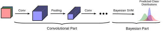
In Section 3.3 we show that our proposed multi-class Bayesian SVM can be learned with gradient-based optimization schemes. This enables us to combine it with various deep learning components such as convolutional layers and extend its applicability to unstructured data as shown in Figure 1. The parameters of the convolution and the variational parameters are jointly learned by means of backpropagation.

Figure 2: Pairwise comparison of the multi-class Bayesian SVM versus the binary Bayesian SVM and SVGP. On average, our proposed multi-class Bayesian SVM provides better results.

4 Experimental Evaluation

In this section we conduct an extensive study of the multi-class Bayesian SVM and analyze its classification performance on structured and unstructured data. Additionally, we analyze the quality of its uncertainty prediction in a large-scale active learning experiment and for the challenging problem of adversarial image detection.

4.1 Classification of Structured Data

Table 1: Mean average rank across 68 data sets. The smaller, the better. Our proposed multi-class Bayesian SVM is on average the most accurate prediction model.

Binary Bayesian SVM	Multi-Class Bayesian SVM	Scalable Variational Gaussian Process
1.96	1.68	2.33

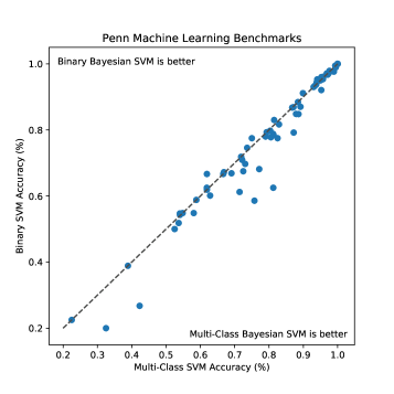
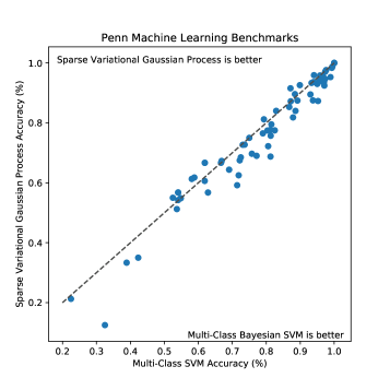
We evaluate the proposed multi-class Bayesian support vector machine with respect to classification accuracy on the Penn Machine Learning Benchmarks [25]. From this benchmark, we select all multi-class classification data sets consisting of at least 128 instances. This subset consists of 68 data sets with up to roughly one million instances. We compare the classification accuracy of our proposed multi-class Bayesian SVM with the most recently proposed binary Bayesian support vector machine [34] (one-vs-rest setup) and the scalable variational Gaussian process (SVGP) [12]. We use the implementation available in GPflow [24] for SVGP and implement the binary and multi-class Bayesian SVM as additional classifiers in GPflow by extending its classifier interface. The shared back end of all three implementations allows a fair training time comparison. For this experiment, all models are trained using 64 inducing points. Gradient-based optimization is performed using Adam [17] with an initial learning rate of $5\cdot 10^{-4}$ for 1000 epochs.

Figure 2 contrasts the multi-class Bayesian SVM with its binary counterpart and SVGP. The proposed multi-class Bayesian SVM clearly outperforms the other two models for most data sets. While this is more pronounced against SVGP, the binary and multi-class Bayesian SVMs exhibit similar behavior. This claim is supported by the comparison of mean ranks (Table 1). The rank per data set is computed by ranking the methods for each data set according to classification accuracy. The most accurate prediction model is assigned rank 1, second best rank 2 and so on. In case of ties, an average rank is used, e.g. if the models exhibit classification accuracies of 1.0, 1.0, and 0.8, they are assigned ranks of 1.5, 1.5, and 3, respectively.

Figure 3: Our proposed multi-class Bayesian SVM clearly needs less time than its competitors.

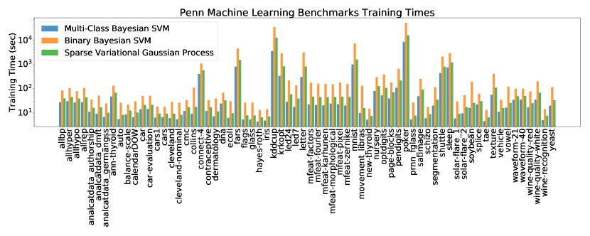
The primary motivation for proposing the multi-class Bayesian SVM is scalability. Classification using the binary Bayesian SVM requires training an independent model per class which increases the training time by a factor equal to the number of classes. Contrastingly, SVGP and our proposed model enable multi-class classification with a single model. This results in significant benefits in training time. As evident in Figure 3, the multi-class Bayesian SVM requires the least training time.

In conclusion, the multi-class Bayesian SVM is the most efficient model without compromising on prediction accuracy. In fact, on average it has a higher accuracy.

4.2 Classification of Image Data

Figure 4: The jointly learned model of a convolutional network and a Bayesian SVM performs as good as a standard network. The price of gaining a Bayesian neural network is a longer training time.

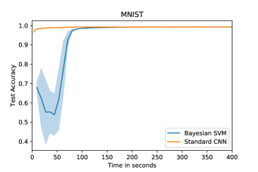
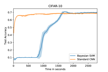
In Section 3.4 we describe how deep learning can be used to learn a feature representation jointly with a multi-class Bayesian SVM. Image data serves as a typical example for unstructured data. We compare the hybrid Bayesian neural network to a standard convolutional neural network (CNN) with a softmax layer for classification. We evaluate these models on two popular image classification benchmarks, MNIST [20] and CIFAR-10 [18].

We observe same performance of the hybrid Bayesian neural network using the Bayesian SVM as a standard CNN with softmax layer. The two different neural networks share the first set of layers, for MNIST: conv(32,5,5)-conv(64,3,3)-max_pool-fc(1024)-fc(100), and for CIFAR-10: conv(128,3,3)-conv(128,3,3)-max_pool-conv(128,3,3)-max_pool-fc(256)-fc(100). As in our previous experiment, we use Adam to perform the optimization.

Figure 4 shows that the hybrid Bayesian neural network achieves the same test accuracy as the standard CNN. The additional training effort of a hybrid Bayesian neural network pays off in achieving probabilistic predictions with uncertainty estimates. While the variational objective and the likelihood exhibits the expected behavior during the training, we note an odd behavior during the initial epochs. We suspect that this is due to initialization of parameters which could result in the KL-term of the variational objective dominating the expected log-likelihood.

4.3 Uncertainty Analysis

One of the advantages of using Bayesian machine learning models lies in getting a distribution over predictions rather than just point-estimates. In this section, we demonstrate this advantage in the domains of active learning and adversarial image detection.

4.3.1 Active Learning

(a) Average rank across 68 data sets.

(b) Representative results for the largest data set.

Figure 5: The Bayesian query policy (variation ratio) decreases the error of the model faster and clearly outperforms the policy based on point-estimates only. For both figures, the smaller the better.

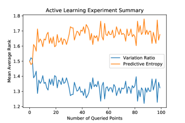
Active learning is concerned with scenarios where the process of labeling data is expensive. In such scenarios, a query policy is adopted to label samples from a large pool of unlabeled instances with the aim to improve model performance. We contrast between two policies to highlight the merits of using prediction uncertainty obtained from the multi-class Bayesian SVM. While the first policy utilizes both mean and variance of the predictive distribution of the Bayesian SVM, the second policy relies only on the mean. For this experiment we use the same data sets as specified in Section 4.1.

We use the variation ratio (VR) as the basis of a Bayesian query policy. It is defined by

$$\text{Variation Ratio}=1-F/S\enspace,$$ (13)

where $F$ is the frequency of the mode and $S$ the number of samples. The VR is the relative number of times the majority class is not predicted. The instance with highest VR is queried. We compare this to a policy which queries the instance with maximum entropy of class probabilities. These are computed using softmax over the mean predictions. For a fair comparison, we the same multi-class Bayesian SVM for both policies. Initially, one instance per class, selected uniformly at random, is labeled. Then, one hundred further instances are queried according to the two policies. As only few training examples are available, we modify the training setup by reducing the number of inducing points to four.

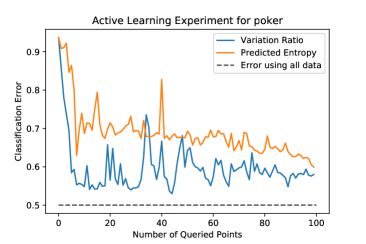
We report the mean average rank across 68 data sets for the two different query policies in Figure 5a. Since both policies start with the same set of labeled instances, the performance is very similar at the beginning. However, with increasing number of queried data points, the Bayesian policy quickly outperforms the other policy. Of the 68 data sets, the poker data set, with more than one million instances, is the largest and consequently the most challenging. Within the first queries, we observe a large decrease in classification error as shown in Figure 5b. We note the same trend of mean ranks across the two policies. The small number of labeled instances is obviously insufficient to reach the test error of a model trained on all data points as shown by the dashed line.

Figure 6: The accuracy on adversarial images decreases with increasing attack strength. A significant increase of the average variation ratio indicates that it is a good feature to detect adversarial images.

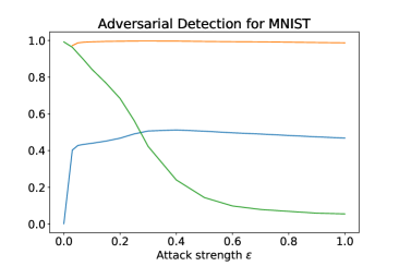
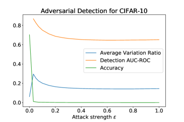
4.3.2 Adversarial Image Detection

With the rise of Deep Learning, its security and reliability is a major concern. A recent development in this direction is the discovery of adversarial images [10]. These correspond to images obtained by adding small imperceptible adversarial noise resulting in high confidence misclassification. While various successful attacks exist, most defense and detection methods do not work [6]. However, Carlini and Wagner [6] acknowledge that the uncertainty obtained from Bayesian machine learning models is the most promising research direction. Several studies show that Bayesian models behave differently for adversarial examples compared to the original data [5, 22, 30, 28]. We take a step further and use the variation ratio (VR) determined by the Bayesian SVM, as defined in Equation (13), for building a detection model for adversarial images.

We attack the hybrid Bayesian neural network described in Section 4.2 with the popular Fast Gradient Sign Method (FGSM) [10]. We generate one adversarial image per image in the test set. We present the results for detection and classification under attack in Figure 6. The Bayesian SVM is not robust to FGSM since its accuracy drops with increasing attack strength $\epsilon$. However, the attack does not remain unperceived. The VR rapidly increases and enables the detection of adversarial images. The ranking of original and adversarial examples with respect to VR yields an ROC-AUC of almost 1 for MNIST. This means that the VR computed for any original example is almost always smaller than the one computed for any adversarial example.

CIFAR-10 exhibits different results under the same setup. Here, the detection is poor and it significantly worsens with increasing attack strength. Potentially, this is an artifact of the poor classification model for CIFAR-10. In contrast to the MNIST classifier, this model is under-confident on original examples. Thus, a weaker attack succeeds in reducing the test accuracy to 1.16%. We believe a better network architecture combined with techniques such as data augmentation will lead to an improved performance in terms of test accuracy and subsequently better detection. Nevertheless, the detection performance of our model is still better than a random detector, even for the strongest attack.

5 Conclusions

We devise a pseudo-likelihood for the multi-class hinge loss leading to the first multi-class Bayesian support vector machine. Additionally, we derive a variational training objective for the proposed model and develop a scalable inference algorithm to optimize it. We establish the efficacy of the model on multi-class classification tasks with extensive experimentation on structured data and contrast its accuracy to two state-of-the-art competitor methods. We provide empirical evidence that our proposed method is on average better and up to an order of magnitude faster to train. Furthermore, we extend our formulation to a hybrid Bayesian neural network and report comparable accuracy to standard models for image classification tasks. Finally, we investigate the key advantage of Bayesian modeling in our approach by demonstrating the use of prediction uncertainty in solving the challenging tasks of active learning and adversarial image detection. The uncertainty-based policy outperforms its competitor in the active learning scenario. Similarly, the uncertainty-enabled adversarial detection shows promising results for image data sets with near-perfect performance on MNIST.

Appendix A Derivation of the Variational Training Objective

We provide a detailed derivation of the proposed variational training objective,

$$\mathcal{O}= \sum_{n=1}^{N}\left(-\frac{1}{2\sqrt{\alpha_{n}}}\left(2\tilde{K}_{n,n}+\left(1+\boldsymbol{\kappa}_{n}\left(\boldsymbol{\mu}_{t_{n}}-\boldsymbol{\mu}_{y_{n}}\right)\right)^{2}+\boldsymbol{\kappa}_{n}\Sigma_{t_{n}}\boldsymbol{\kappa}_{n}^{\intercal}+\boldsymbol{\kappa}_{n}\Sigma_{y_{n}}\boldsymbol{\kappa}_{n}^{\intercal}-\alpha_{n}\right)\right.$$

$$\phantom{\sum_{i=1}^{n}\left(\right)}\left.-\boldsymbol{\kappa}_{n}\left(\boldsymbol{\mu}_{t_{n}}-\boldsymbol{\mu}_{y_{n}}\right)-\frac{1}{4}\log\alpha_{n}-\log\left(B_{\frac{1}{2}}\left(\sqrt{\alpha_{n}}\right)\right)\right)$$

$$\phantom{\sum_{i=1}^{n}\left(\right)}-\frac{1}{2}\sum_{j\in Y}\left(-\log\left|\Sigma_{j}\right|+\text{trace}\left(K^{-1}_{PP}\Sigma_{j}\right)+\boldsymbol{\mu}_{j}^{\intercal}K^{-1}_{PP}\boldsymbol{\mu}_{j}\right)\enspace.$$ (14)

We assume that $\mathbf{f}$ and $\boldsymbol{\lambda}$ are independent $q\left(\mathbf{f},\boldsymbol{\lambda}\right)=\prod_{j\in Y}q\left(\mathbf{f}_{j}\right)\prod_{n=1}^{N}q\left(\lambda_{n}\right)$. Furthermore, we impose a variational sparse approximation where, $q(\mathbf{f}_{j})=\int p(\mathbf{f}_{j}|\mathbf{u}_{j})q(\mathbf{u}_{j})\mathrm{d}\mathbf{u}_{j}$ with $p(\mathbf{f}_{j}|\mathbf{u}_{j})=\mathcal{N}\left(\kappa\mathbf{u}_{j},\tilde{K}\right)$, $q\left(\mathbf{u}_{j}\right)=\mathcal{N}\left(\mathbf{u}_{j}|\boldsymbol{\mu}_{j},\Sigma_{j}\right)$, and $q\left(\lambda_{n}\right)=\mathcal{GIG}\left(\frac{1}{2},1,\alpha_{n}\right)$. We use $p\left(\mathbf{u}_{j}\right)=\mathcal{N}\left(0,K_{PP}\right)$ as a prior on the inducing points. Here, $\kappa=K_{NP}K^{-1}_{PP}$, $\tilde{K}=K_{NN}-K_{NP}K^{-1}_{PP}K_{PN}$, and $t_{n}=\operatorname*{arg\,max}_{t\in Y,t\neq y_{n}}f_{n,t}$. In the following, $t_{n}$ indicates the class index of highest class prediction for a class not equal to the true class $y_{n}$.

The goal of variational inference is to maximize the evidence lower bound (ELBO),

ELBO $$=\mathbb{E}_{q(\mathbf{u},\boldsymbol{\lambda})}\left[\log p\left(\mathbf{y}|\mathbf{u},\boldsymbol{\lambda}\right)\right]-\operatorname{KL}\left[q\left(\mathbf{u},\boldsymbol{\lambda}\right)||p\left(\mathbf{u},\boldsymbol{\lambda}\right)\right]$$ (15)

$$=\mathbb{E}_{q(\mathbf{u},\boldsymbol{\lambda})}[\log p(\mathbf{y}|\mathbf{u},\boldsymbol{\lambda)}]+\mathbb{E}_{q(\mathbf{\mathbf{u}},\boldsymbol{\lambda})}[\log p(\mathbf{u},\boldsymbol{\lambda})]-\mathbb{E}_{q(\mathbf{u},\boldsymbol{\lambda})}[\log q(\mathbf{u},\boldsymbol{\lambda})]$$ (16)

$$=\mathbb{E}_{q(\mathbf{u},\boldsymbol{\lambda})}[\log p(\mathbf{y},\mathbf{u},\boldsymbol{\lambda})]-\mathbb{E}_{q(\mathbf{u},\boldsymbol{\lambda})}[\log q(\mathbf{u},\boldsymbol{\lambda})]$$ (17)

$$=\mathbb{E}_{q(\mathbf{u},\boldsymbol{\lambda})}\left[\log p\left(\mathbf{y},\boldsymbol{\lambda}|\mathbf{u}\right)\right]+\mathbb{E}_{q(\mathbf{u},\boldsymbol{\lambda})}[\log p\left(\mathbf{u}\right)]-\mathbb{E}_{q(\mathbf{u},\boldsymbol{\lambda})}[\log q(\mathbf{u},\boldsymbol{\lambda})]$$ (18)

$$=\mathbb{E}_{q(\mathbf{u},\boldsymbol{\lambda})}\left[\log\left[\mathbb{E}_{p(\mathbf{f}|\mathbf{u})}\left[p\left(\mathbf{y},\boldsymbol{\lambda}|\mathbf{f}\right)\right]\right]\right]+\mathbb{E}_{q(\mathbf{u},\boldsymbol{\lambda})}[\log p\left(\mathbf{u}\right)]-\mathbb{E}_{q(\mathbf{u},\boldsymbol{\lambda})}[\log q(\mathbf{u},\boldsymbol{\lambda})]$$ (19)

We apply Jensen’s inequality to the first term to obtain a tractable lower bound,

$$\log\mathbb{E}_{p\left(\mathbf{f}|\mathbf{u}\right)}\left[p\left(\mathbf{y},\boldsymbol{\lambda}|\mathbf{f}\right)\right]$$ (20)

$$\geq \mathbb{E}_{p\left(\mathbf{f}|\mathbf{u}\right)}\left[\log p\left(\mathbf{y},\boldsymbol{\lambda}|\mathbf{f}\right)\right]$$ (21)

$$= \sum_{n=1}^{N}\mathbb{E}_{p\left(\mathbf{f}|\mathbf{u}\right)}\left[\log p\left(y_{n},\lambda_{n}|\mathbf{f}\right)\right]$$ (22)

$$= \sum_{n=1}^{N}\mathbb{E}_{p\left(\mathbf{f}|\mathbf{u}\right)}\left[\log\left(\frac{1}{\sqrt{2\pi\lambda_{n}}}\exp\left(-\frac{1}{2}\frac{\left(1+\lambda_{n}+f_{t_{n}}\left(\mathbf{x}_{n}\right)-f_{y_{n}}\left(\mathbf{x}_{n}\right)\right)^{2}}{\lambda_{n}}\right)\right)\right]$$ (23)

$$\propto -\frac{1}{2}\sum_{n=1}^{N}\mathbb{E}_{p\left(\mathbf{f}|\mathbf{u}\right)}\left[\log\lambda_{n}+\frac{\left(1+\lambda_{n}+f_{t_{n}}\left(\mathbf{x}_{n}\right)-f_{y_{n}}\left(\mathbf{x}_{n}\right)\right)^{2}}{\lambda_{n}}\right]$$ (24)

$$= -\frac{1}{2}\sum_{n=1}^{N}\log\lambda_{n}+\frac{1}{\lambda_{n}}\mathbb{E}_{p\left(\mathbf{f}|\mathbf{u}\right)}\left[\left(1+\lambda_{n}+f_{t_{n}}\left(\mathbf{x}_{n}\right)-f_{y_{n}}\left(\mathbf{x}_{n}\right)\right)^{2}\right]$$ (25)

$$= -\frac{1}{2}\sum_{n=1}^{N}\log\lambda_{n}+\frac{1}{\lambda_{n}}\left(2\tilde{K}_{n,n}+\left(1+\lambda_{n}+\boldsymbol{\kappa}_{n}\left(\mathbf{u}_{t_{n}}-\mathbf{u}_{y_{n}}\right)\right)^{2}\right)\enspace.$$ (26)

Now we simplify the expectation with respect to the approximate posterior $q(\mathbf{u},\boldsymbol{\lambda})$ as,

$$\mathbb{E}_{q}\left[\log\lambda_{n}+\frac{1}{\lambda_{n}}\left(2\tilde{K}_{n,n}+\left(1+\lambda_{n}+\boldsymbol{\kappa}_{n}\left(\mathbf{u}_{t_{n}}-\mathbf{u}_{y_{n}}\right)\right)^{2}\right)\right]$$ (27)

$$= \mathbb{E}_{q}\left[\log\lambda_{n}\right]+\mathbb{E}_{q}\left[\frac{1}{\lambda_{n}}\left(2\tilde{K}_{n,n}+\left(1+\lambda_{n}+\boldsymbol{\kappa}_{n}\left(\mathbf{u}_{t_{n}}-\mathbf{u}_{y_{n}}\right)\right)^{2}\right)\right]$$ (28)

$$= \mathbb{E}_{q}\left[\log\lambda_{n}\right]+\mathbb{E}_{q}\left[\frac{1}{\lambda_{n}}\left(2\tilde{K}_{n,n}+1+2\lambda_{n}+2\boldsymbol{\kappa}_{n}\left(\mathbf{u}_{t_{n}}-\mathbf{u}_{y_{n}}\right)+\lambda_{n}^{2}+2\lambda_{n}\boldsymbol{\kappa}_{n}\left(\mathbf{u}_{t_{n}}-\mathbf{u}_{y_{n}}\right)\right.\right.$$

$$\phantom{\mathbb{E}_{q}\left[\log\lambda_{n}\right]+\mathbb{E}_{q}\left[\frac{1}{\lambda_{n}}\left(\right)\right]}\left.\left.+\left(\boldsymbol{\kappa}_{n}\mathbf{u}_{t_{n}}\right)^{2}+\left(\boldsymbol{\kappa}_{n}\mathbf{u}_{y_{n}}\right)^{2}-2\boldsymbol{\kappa}_{n}\mathbf{u}_{t_{n}}\boldsymbol{\kappa}_{n}\mathbf{u}_{y_{n}}\right)\right]$$ (29)

$$\propto \mathbb{E}_{q\left(\lambda_{n}\right)}\left[\log\lambda_{n}\right]+\frac{1}{\sqrt{\alpha_{n}}}\left(2\tilde{K}_{n,n}+\left(1+\boldsymbol{\kappa}_{n}\left(\boldsymbol{\mu}_{t_{n}}-\boldsymbol{\mu}_{y_{n}}\right)\right)^{2}+\boldsymbol{\kappa}_{n}\Sigma_{t_{n}}\boldsymbol{\kappa}_{n}^{\intercal}+\boldsymbol{\kappa}_{n}\Sigma_{y_{n}}\boldsymbol{\kappa}_{n}^{\intercal}\right)$$

$$+\mathbb{E}_{q\left(\lambda_{n}\right)}\left[\lambda_{n}\right]+2\boldsymbol{\kappa}_{n}\left(\boldsymbol{\mu}_{t_{n}}-\boldsymbol{\mu}_{y_{n}}\right)\enspace.$$ (30)

Wenzel et al. [34] derive the entropy of $q\left(\lambda_{n}\right)$ as

$$\mathbb{E}_{q\left(\lambda_{n}\right)}\left[\log q\left(\lambda_{n}\right)\right]\propto-\frac{1}{4}\log\left(\alpha_{n}\right)-\frac{1}{2}\mathbb{E}_{q\left(\lambda_{n}\right)}\left[\log\left(\lambda_{n}\right)\right]-\log\left(B_{\frac{1}{2}}\left(\sqrt{\alpha_{n}}\right)\right)-\frac{1}{2}\mathbb{E}_{q\left(\lambda_{n}\right)}\left[\lambda_{n}\right]-\frac{\sqrt{\alpha_{n}}}{2}\enspace,$$ (31)

where $B_{\frac{1}{2}}\left(\cdot\right)$ is the modified Bessel function [16]. Plugging these expressions into the derived lower bound on evidence lower bound leads to our variational training objective,

$$\sum_{n=1}^{N}\left(-\frac{1}{2}\left(\mathbb{E}_{q\left(\lambda_{n}\right)}\left[\log\lambda_{n}\right]+\frac{1}{\sqrt{\alpha_{n}}}\left(2\tilde{K}_{n,n}+\left(1+\boldsymbol{\kappa}_{n}\left(\boldsymbol{\mu}_{t_{n}}-\boldsymbol{\mu}_{y_{n}}\right)\right)^{2}+\boldsymbol{\kappa}_{n}\Sigma_{t_{n}}\boldsymbol{\kappa}_{n}^{\intercal}+\boldsymbol{\kappa}_{n}\Sigma_{y_{n}}\boldsymbol{\kappa}_{n}^{\intercal}\right)\right.\right.$$

$$\phantom{\sum_{i=1}^{n}\left(\right)}\left.+\mathbb{E}_{q\left(\lambda_{n}\right)}\left[\lambda_{n}\right]+2\boldsymbol{\kappa}_{n}\left(\boldsymbol{\mu}_{t_{n}}-\boldsymbol{\mu}_{y_{n}}\right)-\frac{1}{4}\log\alpha_{n}-\frac{1}{2}\mathbb{E}_{q\left(\lambda_{n}\right)}\left[\log\lambda_{n}\right]\right)$$

$$\phantom{\sum_{i=1}^{n}\left(\right)}\left.-\log\left(B_{\frac{1}{2}}\left(\sqrt{\alpha_{n}}\right)\right)-\frac{1}{2}\mathbb{E}_{q\left(\lambda_{n}\right)}\left[\lambda_{n}\right]-\frac{\sqrt{\alpha_{n}}}{2}\right)-\mathrm{KL}\left(q\left(\mathbf{u}\right)\bigparallel p\left(\mathbf{u}\right)\right)$$ (32)

$$=\sum_{n=1}^{N}\left(-\frac{1}{2\sqrt{\alpha_{n}}}\left(2\tilde{K}_{n,n}+\left(1+\boldsymbol{\kappa}_{n}\left(\boldsymbol{\mu}_{t_{n}}-\boldsymbol{\mu}_{y_{n}}\right)\right)^{2}+\boldsymbol{\kappa}_{n}\Sigma_{t_{n}}\boldsymbol{\kappa}_{n}^{\intercal}+\boldsymbol{\kappa}_{n}\Sigma_{y_{n}}\boldsymbol{\kappa}_{n}^{\intercal}-\alpha_{n}\right)\right.$$

$$\phantom{\sum_{i=1}^{n}\left(\right)}\left.-\boldsymbol{\kappa}_{n}\left(\boldsymbol{\mu}_{t_{n}}-\boldsymbol{\mu}_{y_{n}}\right)-\frac{1}{4}\log\alpha_{n}-\log\left(B_{\frac{1}{2}}\left(\sqrt{\alpha_{n}}\right)\right)\right)$$

$$\phantom{\sum_{i=1}^{n}\left(\right)}-\frac{1}{2}\sum_{j\in Y}\left(-\log\left|\Sigma_{j}\right|+\text{trace}\left(K^{-1}_{PP}\Sigma_{j}\right)+\boldsymbol{\mu}_{j}^{\intercal}K^{-1}_{PP}\boldsymbol{\mu}_{j}\right)=\mathcal{O}$$ (33)

Appendix B Derivation of Euclidean Gradients

We derive the Euclidean gradients with respect to $\boldsymbol{\mu}_{j}$, $\Sigma_{j}$ and $\alpha_{n}$ using the notation from the previous section.

$$\frac{\partial\mathcal{O}_{n}}{\partial\boldsymbol{\mu}_{j}} =\frac{\partial}{\partial\boldsymbol{\mu}_{j}}\left[-\frac{1}{2\sqrt{\alpha_{n}}}\left(1+\boldsymbol{\kappa}_{n}\left(\boldsymbol{\mu}_{t_{n}}-\boldsymbol{\mu}_{y_{n}}\right)\right)^{2}-\boldsymbol{\kappa}_{n}\left(\boldsymbol{\mu}_{t_{n}}-\boldsymbol{\mu}_{y_{n}}\right)-\frac{1}{2N}\sum_{j\in Y}\boldsymbol{\mu}_{j}^{\intercal}K_{PP}^{-1}\boldsymbol{\mu}_{j}\right]$$ (34)

$$=\begin{cases}-\frac{1}{\sqrt{\alpha_{n}}}\left(\boldsymbol{\kappa}_{n}^{T}+\boldsymbol{\kappa}_{n}^{T}\boldsymbol{\kappa}_{n}\boldsymbol{\mu}_{j}-\boldsymbol{\kappa}_{n}^{T}\boldsymbol{\kappa}_{n}\boldsymbol{\mu}_{y_{n}}\right)-\boldsymbol{\kappa}_{n}^{T}-\frac{1}{N}K_{PP}^{-1}\boldsymbol{\mu}_{j}&j=t_{n}\\ \frac{1}{\sqrt{\alpha_{n}}}\left(\boldsymbol{\kappa}_{n}^{T}+\boldsymbol{\kappa}_{n}^{T}\boldsymbol{\kappa}_{n}\boldsymbol{\mu}_{t_{n}}-\boldsymbol{\kappa}_{n}^{T}\boldsymbol{\kappa}_{n}\boldsymbol{\mu}_{j}\right)+\boldsymbol{\kappa}_{n}^{T}-\frac{1}{N}K_{PP}^{-1}\boldsymbol{\mu}_{j}&j=y_{n}\\ -\frac{1}{N}K_{PP}^{-1}\boldsymbol{\mu}_{j}&\text{otherwise}\end{cases}$$ (35)

$$\frac{\partial\mathcal{O}_{n}}{\partial\Sigma_{j}} =\frac{\partial}{\partial\Sigma_{j}}\left[-\frac{1}{2\sqrt{\alpha_{n}}}\left(\boldsymbol{\kappa}_{n}\Sigma_{y_{n}}\boldsymbol{\kappa}_{n}^{\intercal}+\boldsymbol{\kappa}_{n}\Sigma_{t_{n}}\boldsymbol{\kappa}_{n}^{\intercal}\right)-\frac{1}{2N}\sum_{j\in Y}\left(-\log\left|\Sigma_{j}\right|+\text{trace}\left(K_{PP}^{-1}\Sigma_{j}\right)\right)\right]$$ (36)

$$=\begin{cases}-\frac{1}{2\sqrt{\alpha_{n}}}\boldsymbol{\kappa}_{n}^{T}\boldsymbol{\kappa}_{n}-\frac{1}{2N}\left(-\Sigma_{j}^{-1}+K_{PP}^{-1}\right)&j=t_{n}\lor j=y_{n}\\ -\frac{1}{2N}\left(-\Sigma_{j}^{-1}+K_{PP}^{-1}\right)&\text{otherwise}\end{cases}$$ (37)

$$\frac{\partial\mathcal{O}}{\partial\alpha_{n}} =\frac{\partial}{\partial\alpha_{n}}\left[-\frac{1}{2\sqrt{\alpha_{n}}}\left(2\tilde{K}_{n,n}+\left(1+\boldsymbol{\kappa}_{n}\left(\boldsymbol{\mu}_{t_{n}}-\boldsymbol{\mu}_{y_{n}}\right)\right)^{2}+\boldsymbol{\kappa}_{n}\Sigma_{y_{n}}\boldsymbol{\kappa}_{n}^{\intercal}+\boldsymbol{\kappa}_{n}\Sigma_{t_{n}}\boldsymbol{\kappa}_{n}^{\intercal}-\alpha_{n}\right)\right.$$

$$\phantom{\frac{\partial}{\partial\alpha_{n}}\left[\frac{1}{1}\right]}\left.-\frac{1}{4}\log\alpha_{n}-\log\left(B_{\frac{1}{2}}\left(\sqrt{\alpha_{n}}\right)\right)\right]$$ (38)

$$=\frac{1}{4\sqrt{\alpha_{n}}^{3}}\left(2\tilde{K}_{n,n}+\left(1+\boldsymbol{\kappa}_{n}\left(\boldsymbol{\mu}_{t_{n}}-\boldsymbol{\mu}_{y_{n}}\right)\right)^{2}+\boldsymbol{\kappa}_{n}\Sigma_{y_{n}}\boldsymbol{\kappa}_{n}^{\intercal}+\boldsymbol{\kappa}_{n}\Sigma_{t_{n}}\boldsymbol{\kappa}_{n}^{\intercal}\right)+\frac{1}{4\sqrt{\alpha_{n}}}$$

$$\phantom{=}+\frac{1}{4\alpha_{n}}-\left(\frac{1}{4\alpha_{n}}+\frac{1}{2\sqrt{\alpha_{n}}}\right)$$ (39)

$$=\frac{1}{4\sqrt{\alpha_{n}}^{3}}\left(2\tilde{K}_{n,n}+\left(1+\boldsymbol{\kappa}_{n}\left(\boldsymbol{\mu}_{t_{n}}-\boldsymbol{\mu}_{y_{n}}\right)\right)^{2}+\boldsymbol{\kappa}_{n}\Sigma_{y_{n}}\boldsymbol{\kappa}_{n}^{\intercal}+\boldsymbol{\kappa}_{n}\Sigma_{t_{n}}\boldsymbol{\kappa}_{n}^{\intercal}\right)-\frac{1}{4\sqrt{\alpha_{n}}}$$ (40)

Appendix C Inference with Coordinate Ascent

Algorithm 1 Coordinate Ascent for inferring variational parameters of Multi-Class Bayesian SVM

0:  Data set $D=\{x_{n},y_{n}\}_{n=1}^{N}$, learning rate $\rho_{t}$, initial inducing points

1:  Compute $\tilde{K}$, $K_{NP}$ and $K_{PP}$.

2:  for $t=1,\ldots,T$ do

3:     for $n=1,\ldots,N$ do

4:        $\alpha_{n}\leftarrow 2\tilde{K}_{n,n}+\left(1+\boldsymbol{\kappa}_{n}\left(\boldsymbol{\mu}_{t_{n}}-\boldsymbol{\mu}_{y_{n}}\right)\right)^{2}+\boldsymbol{\kappa}_{n}\Sigma_{y_{n}}\boldsymbol{\kappa}_{n}^{\intercal}+\boldsymbol{\kappa}_{n}\Sigma_{t_{n}}\boldsymbol{\kappa}_{n}^{\intercal}$.

5:     for $j\in Y$ do

6:        Compute $\hat{\boldsymbol{\eta}}_{1,j}$ according to Equation (45).

7:        Compute $\hat{\boldsymbol{\eta}}_{2,j}$ according to Equation (46).

8:        $\boldsymbol{\eta}_{1,j}\leftarrow\left(1-\rho_{t}\right)\boldsymbol{\eta}_{1,j}+\rho_{t}\hat{\boldsymbol{\eta}}_{1,j}$

9:        $\boldsymbol{\eta}_{2,j}\leftarrow\left(1-\rho_{t}\right)\boldsymbol{\eta}_{2,j}+\rho_{t}\hat{\boldsymbol{\eta}}_{2,j}$

10:        $\Sigma_{j}\leftarrow-\frac{1}{2}\boldsymbol{\eta}_{2,j}^{-1}$

11:        $\mu_{j}\leftarrow\Sigma_{j}\boldsymbol{\eta}_{1,j}$

12:  return  $\alpha$, $\mu$, $\Sigma$

Wenzel et al. [34] propose the use of coordinate ascent in order to speed up the inference. While we relied in our experiments on Euclidean gradients combined with stochastic gradient ascent based algorithms, this inference scheme is also applicable for our proposed multi-class inference. For completeness we derive this algorithm as well.

First, we require to derive the natural gradients by multiplying the Euclidean gradients with the inverse Fisher information matrix [1]. Since we apply it to a Gaussian distribution, this results in the following natural gradients

$$\widetilde{\nabla}_{\boldsymbol{\eta}_{1,j},\boldsymbol{\eta}_{2,j}}\mathcal{O}_{n}=\left(\frac{\partial\mathcal{O}_{n}}{\partial\boldsymbol{\mu}_{j}}-2\frac{\partial\mathcal{O}_{n}}{\partial\Sigma_{j}}\boldsymbol{\mu}_{j},\ \frac{\partial\mathcal{O}_{n}}{\partial\Sigma_{j}}\right)$$

Using the identities $\boldsymbol{\eta}_{1,j}=\Sigma_{j}^{-1}\boldsymbol{\mu}_{j}$ and $\boldsymbol{\eta}_{2,j}=-\frac{1}{2}\Sigma_{j}^{-1}$, we derive the final natural gradients,

$$\widetilde{\nabla}_{\boldsymbol{\eta}_{2,j}}\mathcal{O}_{n} =-\frac{1}{2N}\left(-2\boldsymbol{\eta}_{2,j}+K_{PP}^{-1}\right)-\begin{cases}\frac{1}{2\sqrt{\alpha_{n}}}\boldsymbol{\kappa}_{n}^{T}\boldsymbol{\kappa}_{n}&j=t_{n}\lor j=y_{n}\\ 0&\text{otherwise}\end{cases}$$ (41)

$$\widetilde{\nabla}_{\boldsymbol{\eta}_{1,j}}\mathcal{O}_{n} =\left(\frac{1}{\sqrt{\alpha_{n}}}\left(\boldsymbol{\kappa}_{n}^{T}+\frac{1}{2}\boldsymbol{\kappa}_{n}^{T}\boldsymbol{\kappa}_{n}\boldsymbol{\eta}_{2,t_{n}}^{-1}\boldsymbol{\eta}_{1,t_{n}}-\frac{1}{2}\boldsymbol{\kappa}_{n}^{T}\boldsymbol{\kappa}_{n}\boldsymbol{\eta}_{2,y_{n}}^{-1}\boldsymbol{\eta}_{1,y_{n}}\right)+\boldsymbol{\kappa}_{n}^{T}\right)\cdot\begin{cases}-1&j=t_{n}\\ 1&j=y_{n}\\ 0&\text{otherwise}\end{cases}$$

$$-\frac{1}{2N}K_{PP}^{-1}\boldsymbol{\eta}_{2,j}^{-1}\boldsymbol{\eta}_{1,j}$$

$$-2\left(-\frac{1}{2N}\left(-2\boldsymbol{\eta}_{2,j}+K_{PP}^{-1}\right)-\begin{cases}\frac{1}{2\sqrt{\alpha_{n}}}\boldsymbol{\kappa}_{n}^{T}\boldsymbol{\kappa}_{n}&j=t_{n}\lor j=y_{n}\\ 0&\text{otherwise}\end{cases}\right)\frac{1}{2}\boldsymbol{\eta}_{2,j}^{-1}\boldsymbol{\eta}_{1,j}$$ (42)

$$=-\frac{1}{N}\boldsymbol{\eta}_{1,j}+\begin{cases}-\left(\frac{1}{\sqrt{\alpha_{n}}}\left(\boldsymbol{\kappa}_{n}^{T}-\frac{1}{2}\boldsymbol{\kappa}_{n}^{T}\boldsymbol{\kappa}_{n}\boldsymbol{\eta}_{2,y_{n}}^{-1}\boldsymbol{\eta}_{1,y_{n}}\right)+\boldsymbol{\kappa}_{n}^{T}\right)&j=t_{n}\\ \left(\frac{1}{\sqrt{\alpha_{n}}}\left(\boldsymbol{\kappa}_{n}^{T}+\frac{1}{2}\boldsymbol{\kappa}_{n}^{T}\boldsymbol{\kappa}_{n}\boldsymbol{\eta}_{2,t_{n}}^{-1}\boldsymbol{\eta}_{1,t_{n}}\right)+\boldsymbol{\kappa}_{n}^{T}\right)&j=y_{n}\\ 0&\text{otherwise}\end{cases}$$ (43)

$$=-\frac{1}{N}\boldsymbol{\eta}_{1,j}+\boldsymbol{\kappa}_{n}^{T}\begin{cases}-\left(\frac{1}{\sqrt{\alpha_{n}}}\left(1-\frac{1}{2}\boldsymbol{\kappa}_{n}\boldsymbol{\eta}_{2,y_{n}}^{-1}\boldsymbol{\eta}_{1,y_{n}}\right)+1\right)&j=t_{n}\\ \left(\frac{1}{\sqrt{\alpha_{n}}}\left(1+\frac{1}{2}\boldsymbol{\kappa}_{n}\boldsymbol{\eta}_{2,t_{n}}^{-1}\boldsymbol{\eta}_{1,t_{n}}\right)+1\right)&j=y_{n}\\ 0&\text{otherwise}\end{cases}$$ (44)

Equating the gradients to zero yields the following update rules

$$\boldsymbol{\eta}_{1,j} =-N\boldsymbol{\kappa}_{n}^{T}\begin{cases}-\left(\frac{1}{\sqrt{\alpha_{n}}}\left(1-\frac{1}{2}\boldsymbol{\kappa}_{n}\boldsymbol{\eta}_{2,y_{n}}^{-1}\boldsymbol{\eta}_{1,y_{n}}\right)+1\right)&j=t_{n}\\ \left(\frac{1}{\sqrt{\alpha_{n}}}\left(1+\frac{1}{2}\boldsymbol{\kappa}_{n}\boldsymbol{\eta}_{2,t_{n}}^{-1}\boldsymbol{\eta}_{1,t_{n}}\right)+1\right)&j=y_{n}\\ 0&\text{otherwise}\end{cases}$$ (45)

$$\boldsymbol{\eta}_{2,j} =-\frac{1}{2}K_{PP}^{-1}-N\begin{cases}\frac{1}{2\sqrt{\alpha_{n}}}\boldsymbol{\kappa}_{n}^{T}\boldsymbol{\kappa}_{n}&j=t_{n}\lor j=y_{n}\\ 0&\text{otherwise}\end{cases}$$ (46)

Finally, we summarize the inference algorithm in Algorithm 1. For training the remaining parameters such as inducing point locations and kernel hyperparameters, we propose to use standard gradient updates after every few coordinate ascent steps. This learning of hyperparameters is often referred to as Type II maximum likelihood [27].

References

• Amari and Nagaoka [2007] Shun-ichi Amari and Hiroshi Nagaoka. Methods of information geometry, volume 191. American Mathematical Soc., 2007.
• Andrews and Mallows [1974] D. F. Andrews and C. L. Mallows. Scale mixtures of normal distributions. Journal of the Royal Statistical Society. Series B (Methodological), 36(1):99–102, 1974. ISSN 00359246. URL http://www.jstor.org/stable/2984774.
• Blei et al. [2016] David M. Blei, Alp Kucukelbir, and Jon D. McAuliffe. Variational inference: A review for statisticians. CoRR, abs/1601.00670, 2016. URL http://arxiv.org/abs/1601.00670.
• Boser et al. [1992] Bernhard E. Boser, Isabelle Guyon, and Vladimir Vapnik. A training algorithm for optimal margin classifiers. In Proceedings of the Fifth Annual ACM Conference on Computational Learning Theory, COLT 1992, Pittsburgh, PA, USA, July 27-29, 1992., pages 144–152, 1992. doi: 10.1145/130385.130401. URL http://doi.acm.org/10.1145/130385.130401.
• Bradshaw et al. [2017] John Bradshaw, Alexander G. de G. Matthews, and Zoubin Ghahramani. Adversarial examples, uncertainty, and transfer testing robustness in gaussian process hybrid deep networks, 2017.
• Carlini and Wagner [2017] Nicholas Carlini and David Wagner. Adversarial examples are not easily detected: Bypassing ten detection methods, 2017.
• Cortes and Vapnik [1995] Corinna Cortes and Vladimir Vapnik. Support-vector networks. Machine Learning, 20(3):273–297, 1995. doi: 10.1007/BF00994018. URL https://doi.org/10.1007/BF00994018.
• Crammer and Singer [2001] Koby Crammer and Yoram Singer. On the algorithmic implementation of multiclass kernel-based vector machines. Journal of Machine Learning Research, 2:265–292, 2001. URL http://www.jmlr.org/papers/v2/crammer01a.html.
• Dogan et al. [2016] Ürün Dogan, Tobias Glasmachers, and Christian Igel. A unified view on multi-class support vector classification. Journal of Machine Learning Research, 17:45:1–45:32, 2016. URL http://jmlr.org/papers/v17/11-229.html.
• Goodfellow et al. [2014] Ian J. Goodfellow, Jonathon Shlens, and Christian Szegedy. Explaining and harnessing adversarial examples, 2014.
• Henao et al. [2014] Ricardo Henao, Xin Yuan, and Lawrence Carin. Bayesian nonlinear support vector machines and discriminative factor modeling. In Advances in Neural Information Processing Systems, pages 1754–1762, 2014.
• Hensman et al. [2015] James Hensman, Alexander G. de G. Matthews, and Zoubin Ghahramani. Scalable variational gaussian process classification. In Proceedings of the Eighteenth International Conference on Artificial Intelligence and Statistics, AISTATS 2015, San Diego, California, USA, May 9-12, 2015, 2015. URL http://jmlr.org/proceedings/papers/v38/hensman15.html.
• Hofmann et al. [2008] T. Hofmann, B. Schölkopf, and AJ. Smola. Kernel methods in machine learning. Annals of Statistics, 36(3):1171–1220, June 2008.
• Jones et al. [1998] Donald R. Jones, Matthias Schonlau, and William J. Welch. Efficient global optimization of expensive black-box functions. J. Global Optimization, 13(4):455–492, 1998. doi: 10.1023/A:1008306431147. URL https://doi.org/10.1023/A:1008306431147.
• Jordan et al. [1999] Michael I. Jordan, Zoubin Ghahramani, Tommi S. Jaakkola, and Lawrence K. Saul. An introduction to variational methods for graphical models. Machine Learning, 37(2):183–233, 1999. doi: 10.1023/A:1007665907178. URL https://doi.org/10.1023/A:1007665907178.
• Jørgensen [1982] Bent Jørgensen. Statistical properties of the generalized inverse Gaussian distribution. Number 9 in Lecture notes in statistics. Springer, New York, NY [u.a.], 1982. ISBN 0387906657.
• Kingma and Ba [2014] Diederik P. Kingma and Jimmy Ba. Adam: A method for stochastic optimization. CoRR, abs/1412.6980, 2014. URL http://arxiv.org/abs/1412.6980.
• Krizhevsky [2009] Alex Krizhevsky. Learning multiple layers of features from tiny images. Technical report, 2009.
• Kuss and Rasmussen [2005] Malte Kuss and Carl Edward Rasmussen. Assessing approximate inference for binary gaussian process classification. Journal of Machine Learning Research, 6:1679–1704, 2005. URL http://www.jmlr.org/papers/v6/kuss05a.html.
• LeCun and Cortes [2010] Yann LeCun and Corinna Cortes. MNIST handwritten digit database. 2010. URL http://yann.lecun.com/exdb/mnist/.
• Li et al. [2010] Lihong Li, Wei Chu, John Langford, and Robert E. Schapire. A contextual-bandit approach to personalized news article recommendation. In Proceedings of the 19th International Conference on World Wide Web, WWW 2010, Raleigh, North Carolina, USA, April 26-30, 2010, pages 661–670, 2010. doi: 10.1145/1772690.1772758. URL http://doi.acm.org/10.1145/1772690.1772758.
• Li and Gal [2017] Yingzhen Li and Yarin Gal. Dropout inference in bayesian neural networks with alpha-divergences. In Proceedings of the 34th International Conference on Machine Learning, ICML 2017, Sydney, NSW, Australia, 6-11 August 2017, pages 2052–2061, 2017. URL http://proceedings.mlr.press/v70/li17a.html.
• Luts and Ormerod [2014] Jan Luts and John T. Ormerod. Mean field variational bayesian inference for support vector machine classification. Computational Statistics & Data Analysis, 73:163–176, 2014. doi: 10.1016/j.csda.2013.10.030. URL https://doi.org/10.1016/j.csda.2013.10.030.
• Matthews et al. [2017] Alexander G. de G. Matthews, Mark van der Wilk, Tom Nickson, Keisuke. Fujii, Alexis Boukouvalas, Pablo León-Villagrá, Zoubin Ghahramani, and James Hensman. GPflow: A Gaussian process library using TensorFlow. Journal of Machine Learning Research, 18(40):1–6, apr 2017. URL http://jmlr.org/papers/v18/16-537.html.
• Olson et al. [2017] Randal S. Olson, William La Cava, Patryk Orzechowski, Ryan J. Urbanowicz, and Jason H. Moore. Pmlb: a large benchmark suite for machine learning evaluation and comparison. BioData Mining, 10(1):36, Dec 2017. ISSN 1756-0381. doi: 10.1186/s13040-017-0154-4. URL https://doi.org/10.1186/s13040-017-0154-4.
• Polson et al. [2011] Nicholas G Polson, Steven L Scott, et al. Data augmentation for support vector machines. Bayesian Analysis, 6(1):1–23, 2011.
• Rasmussen and Williams [2006] Carl Edward Rasmussen and Christopher K. I. Williams. Gaussian processes for machine learning. Adaptive computation and machine learning. MIT Press, 2006. ISBN 026218253X.
• Rawat et al. [2017] Ambrish Rawat, Martin Wistuba, and Maria-Irina Nicolae. Adversarial phenomenon in the eyes of bayesian deep learning. arXiv preprint arXiv:1711.08244, 2017.
• Settles [2009] Burr Settles. Active learning literature survey. Computer Sciences Technical Report 1648, University of Wisconsin–Madison, 2009.
• Smith and Gal [2018] Lewis Smith and Yarin Gal. Understanding measures of uncertainty for adversarial example detection. arXiv preprint arXiv:1803.08533, 2018.
• Snelson and Ghahramani [2005] Edward Snelson and Zoubin Ghahramani. Sparse gaussian processes using pseudo-inputs. In Advances in Neural Information Processing Systems 18 [Neural Information Processing Systems, NIPS 2005, December 5-8, 2005, Vancouver, British Columbia, Canada], pages 1257–1264, 2005. URL http://papers.nips.cc/paper/2857-sparse-gaussian-processes-using-pseudo-inputs.
• Snoek et al. [2012] Jasper Snoek, Hugo Larochelle, and Ryan P. Adams. Practical bayesian optimization of machine learning algorithms. In Advances in Neural Information Processing Systems 25: 26th Annual Conference on Neural Information Processing Systems 2012. Proceedings of a meeting held December 3-6, 2012, Lake Tahoe, Nevada, United States., pages 2960–2968, 2012. URL http://papers.nips.cc/paper/4522-practical-bayesian-optimization-of-machine-learning-algorithms.
• Titsias [2009] Michalis K. Titsias. Variational learning of inducing variables in sparse gaussian processes. In Proceedings of the Twelfth International Conference on Artificial Intelligence and Statistics, AISTATS 2009, Clearwater Beach, Florida, USA, April 16-18, 2009, pages 567–574, 2009. URL http://www.jmlr.org/proceedings/papers/v5/titsias09a.html.
• Wenzel et al. [2017] Florian Wenzel, Théo Galy-Fajou, Matthäus Deutsch, and Marius Kloft. Bayesian nonlinear support vector machines for big data. In Joint European Conference on Machine Learning and Knowledge Discovery in Databases, pages 307–322. Springer, 2017.
• Williams and Barber [1998] Christopher K. I. Williams and David Barber. Bayesian classification with gaussian processes. IEEE Trans. Pattern Anal. Mach. Intell., 20(12):1342–1351, 1998. doi: 10.1109/34.735807. URL https://doi.org/10.1109/34.735807.
• Wistuba et al. [2018] Martin Wistuba, Nicolas Schilling, and Lars Schmidt-Thieme. Scalable gaussian process-based transfer surrogates for hyperparameter optimization. Machine Learning, 107(1):43–78, 2018. doi: 10.1007/s10994-017-5684-y. URL https://doi.org/10.1007/s10994-017-5684-y.