Fault-Tolerant Control of Linear Quantum Stochastic Systems

Abstract

In quantum engineering, faults may occur in a quantum control system, which will cause the quantum control system unstable or deteriorate other relevant performance of the system. This note presents an estimator-based fault-tolerant control design approach for a class of linear quantum stochastic systems subject to fault signals. In this approach, the fault signals and some commutative components of the quantum system observables are estimated, and a fault-tolerant controller is designed to compensate the effect of the fault signals. Numerical procedures are developed for controller design and an example is presented to demonstrate the proposed design approach.

Index Terms— Linear quantum stochastic system, quantum control, fault-tolerant control.

I Introduction

Developing quantum control theory has been recognized a key task due to its potential application in emerging quantum technology [1], [2], [3]. Some control methods such as optimal control [3], $H^{\infty}$ control [4], feedback control [1] have been employed for enhancing the performance in quantum control systems. For practical quantum systems, the stochastic fluctuations in magnetic or electric fields or fault operations on the generators of quantum resources may introduce fault signals that will deteriorate the performance of quantum systems or result in instability [5]-[8]. For example, classical (non-quantum) fault signals may originate from the change in environmental conditions (e.g., temperature) or the voltage fluctuation in controlling a laser generator. It is thus expected to develop fault-tolerant control theory for quantum systems. Most classical fault-tolerant control methods [9]-[11] cannot be straightforwardly applied to quantum control problems due to some unique characteristics of quantum systems such as measurement collapse and non-commutative observables [3]. However, some ideas of estimator-based design in classical control can be adapted to quantum control problems. In [8], fault-tolerant quantum filtering theory has been presented using the concept of quantum-classical conditional expectation. In this note, we present a systematic fault-tolerant control design method for a class of linear quantum stochastic systems subject to faults.

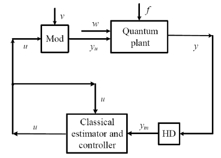
Figure 1: A closed-loop system with an estimator-based fault-tolerant controller. HD represents a homodyne detector for measurements and Mod represents a modulator.

Linear quantum stochastic systems widely exist in quantum optics [4], [12], [13]. Quantum optical components such as beam splitters, squeezers, phase shifters can be used to construct quantum networks for quantum information processing [14]. Some control methods involving coherent feedback [4], [15] and measurement-based feedback [1] have been used for enhancing the performance of linear quantum optical systems with uncertainties. The design problems of robust controllers or observers have also been investigated for uncertain linear quantum stochastic systems [16], [17]. For example, Yamamoto [17] presented the result of robust observer design for linear quantum systems. In particular, a class of linear quantum systems subject to time-varying norm-bounded parametric uncertainties was considered in [17] and a robust observer was proposed to guarantee the variance of the estimation error to be within a certain bound. Here, we develop an estimator-based approach for fault tolerant control design of linear quantum stochastic systems involving measurement-based feedback where we assume that the classical fault signal is independent of quantum noise. Different from uncertainties in the system Hamiltonian and the system operator considered in [17], we consider the classical fault signals in quantum systems and design a controller to compensate the effect of fault signals. We aim to develop a fault-tolerant control design approach with a reduced-order dynamic estimator for a class of quantum systems subject to faults while Yamamoto [17] aimed at designing a robust full-order estimator for a class of quantum systems with uncertainties. The basic idea is illustrated in Fig. 1, where the meaning of different quantities will be explained in Section III. A quantum optical plant subject to fault signals $f$ is measured using a homodyne detector (HD) [1]. The output $y_{m}$ of the HD is used to establish a classical estimator and a classical controller for compensating the effect of $f$ on the quantum optical plant.

This note is organized as follows. Section II introduces some notations and gives a brief overview of linear quantum stochastic systems. Section III presents the setup of closed-loop systems with input faults. The main results for the closed systems subject to input faults are provided in Section IV. Section V proposes numerical approaches for the estimator-based fault-tolerant controller design and illustrates the proposed approaches using an example. Section VI concludes this note.

II Preliminaries

II-A Notation

The notations used in this note are as follows: $i=\sqrt{-1}$; the commutator is defined by $[A,B]=AB-BA$. If $x$ and $y$ are column vectors of operators, the commutator is defined by $[x,y^{T}]=xy^{T}-(yx^{T})^{T}$. If $X=[x_{jk}]$ is a matrix of linear operators or complex numbers, then $X^{\#}=[x^{*}_{jk}]$ denotes the operation of taking the adjoint of each element of $X$, and $X^{{\dagger}}=[x^{*}_{jk}]^{T}$. $\parallel\!X\!\parallel$ represents Euclidean norm of $X$. We define $J={\small\left[\!\!\!\begin{array}[]{cc}0&1\\ -1&0\\ \end{array}\!\!\!\right]}$, and $\mathrm{diag}_{n}(M)$ denotes a block diagonal matrix with a square matrix $M$ appearing $n$ times on the diagonal block. The symbol $I_{n}$ denotes the $n\times n$ identity matrix. $0_{n\times m}$ denotes the $n\times m$ zero matrix, where $n$ and $m$ can be determined from the context when the subscript is omitted.

II-B Linear quantum stochastic systems and physical realizability

Following [4], an open quantum system involving $n$ one degree of freedom open quantum harmonic oscillators coupled to $m$ independent boson fields (e.g., optical beams) is described by linear differential equations of the form

$$dx(t)= Ax(t)dt+Bdw(t),$$

$$dy(t)= Cx(t)dt+Ddw(t),$$ (1)

where $x=[q_{1},p_{1},q_{2},p_{2},\cdots,q_{n},p_{n}]^{T}$ with position operators $q_{j}$ and momentum operators $p_{j}$ ($j=1,\ldots,n$) describes a vector of self-adjoint possibly non-commutative system observables and the non-commutation relation is defined as $xx^{T}-(xx^{T})^{T}=2i\Theta$ with $\Theta=\mathrm{diag}_{n}(J)$. The boson fields $w=[w_{q_{1}},w_{p_{1}},w_{q_{2}},w_{p_{2}},\cdots,w_{q_{m}},w_{p_{m}}]^{T}$ with analogous field operators $w_{q_{k}}(t)$, $w_{p_{k}}(t)$, ($k=1,\ldots,m$) represent the input signal written as

$$dw(t)dw(t)^{T}=F_{w}dt$$ (2)

with $F_{w}=I_{2m}+i\mathrm{diag}_{m}(J)$. Commutation relations for the quantum field components of $w$ may be denoted by:

$$[dw(t),dw(t)^{T}]=(F_{w}-F_{w}^{T})dt=2i\Theta_{w}dt.$$

Commutation relation for the output $y$ is given by

$$[dy(t),dy(t)^{T}]=2i\Theta_{y}dt.$$

The system matrices $A$, $B$, $C$ and $D$ are real constant matrices of suitable dimension. The system matrices must satisfy physical realizability conditions [18], [19] (i) $A\Theta+\Theta A^{T}+B\Theta_{w}B^{T}=0$; (ii) $B\Theta_{w}D^{T}=-\Theta C^{T}$; (iii) $D\Theta_{w}D^{T}=\Theta_{y}$.

III Model Description and Problem Formulation

This section presents a quantum optical plant with input faults, designs an estimator-based fault-tolerant controller and introduces the setup of a closed-loop system.

Consider a quantum plant with fault signals described by a non-commutative stochastic model of the following form:

$$dx(t)= Ax(t)dt+B_{w}dw(t)+B_{u}y_{u}(t)dt+B_{f}f(t)dt,$$

$$dy(t)= Cx(t)dt+Ddw(t),$$ (3)

where $A\in\mathbb{R}^{n\times n}$, $B_{w}\in\mathbb{R}^{n\times n_{w}}$, $B_{u}\in\mathbb{R}^{n\times n_{u}}$, $B_{f}\in\mathbb{R}^{n\times n_{f}}$, $C\in\mathbb{R}^{n_{y}\times n}$, $D\in\mathbb{R}^{n_{y}\times n_{w}}$ ($n$, $n_{w}$, $n_{u}$ and $n_{y}$ are even). $A$, $B=[B_{w}\ B_{u}]$, $C$ and $D$ should satisfy physical realizability conditions. $x$ represents a vector of plant variables and $w$ is the vector of vacuum quantum fields. $B_{f}$ is known and the real column vector $f(t)$ represents the unknown fault signal to be estimated. For example, $f(t)$ may originate from the voltage fluctuation in controlling the laser generator, malfunction of beam splitters, phase shifters, etc. The signal $y_{u}(t)$ is a control input of the form

$$y_{u}(t)= u(0)+\int^{t}_{0}u(s)ds+v(t),$$ (4)

where $v\in\mathbb{R}^{n_{u}}$ and $w$ are independent and $n_{u}$ is even; $u$ and $v$ are the signal and quantum noise parts of $y_{u}$, respectively. When the quantum output signals $y(t)$ are measured by homodyne detectors (HD), classical signals $y_{m}(t)=Gy(t)\in\mathbb{R}^{n_{y_{m}}}$ are produced. The matrix $G$ corresponding to measurement processes satisfies the condition below [20]:

$$G\Theta_{y}G^{T}=0$$ (5)

with $\mathrm{rank}(G)\leq\frac{n_{y}}{2}$, where $G$ represents a static linear transformation (measurement processes) that converts boson fields into classical signals.

Now, we give the following assumption and lemma in this work.

Assumption 1

The fault signal $f(t)$ satisfies $\parallel f(t)\parallel\leq\alpha$ and $\parallel\dot{f}(t)\parallel\leq\beta$, where $\alpha>0$, $\beta>0$.

Lemma 1

Given a quantum optical plant with a fault signal of the form (III), there always exists a permutation matrix $T$ such that the transformed system is given as

$$d\tilde{x}(t)= \tilde{A}\tilde{x}(t)dt+\tilde{B}_{w}dw(t)+\tilde{B}_{u}y_{u}(t)dt+\tilde{B}_{f}f(t)dt,$$

$$dy(t)= \tilde{C}\tilde{x}(t)dt+\tilde{D}dw(t)$$ (6)

with system matrices $\tilde{A}=TAT^{-1}=\left[\begin{array}[]{cc}\tilde{A}_{11}&\tilde{A}_{12}\\ \tilde{A}_{21}&\tilde{A}_{22}\\ \end{array}\right]$, $\tilde{B}_{w}=TB_{w}=\left[\tilde{B}_{w_{1}}^{T}\ \tilde{B}_{w_{2}}^{T}\right]^{T}$, $\tilde{B}_{u}=TB_{u}=\left[\tilde{B}_{u_{1}}^{T}\ \tilde{B}_{u_{2}}^{T}\right]^{T}$, $\tilde{B}_{f}=TB_{f}=\left[\tilde{B}_{f_{1}}^{T}\ \tilde{B}_{f_{2}}^{T}\right]^{T}$, $\tilde{C}=CT^{-1}=[\tilde{C}_{1}\quad\tilde{C}_{2}]$, $\tilde{D}=D$ and new defined system variables $\tilde{x}(t)=Tx(t)=[\tilde{x}_{uo}(t)^{T}\quad\tilde{x}_{o}(t)^{T}]^{T}$, where $\tilde{x}_{o}\in\mathbb{R}^{n_{o}}$ represents $n_{o}$ components of $\tilde{x}(t)$ to be estimated while $\tilde{x}_{uo}\in\mathbb{R}^{n-n_{o}}$ represents unestimated components. Here $n_{o}\leq\frac{n}{2}$ and $\tilde{x}_{o}$ should satisfy $[\tilde{x}_{o}(t),\tilde{x}_{o}(t)^{T}]=0$ for all $t\geq 0$, so that the components of $\tilde{x}_{o}$ can be simultaneously observed.

Let $\eta=\left[\tilde{x}_{uo}^{T}\ \tilde{x}_{o}^{T}\ f^{T}\right]^{T}$ and $h(t)=\frac{df(t)}{dt}$. We first design an augmented system for (1) given by

$$d\eta(t)= \mathcal{A}\eta(t)dt+\mathcal{B}_{w}dw(t)+\mathcal{B}_{u}dy_{u}(t)+\mathcal{B}_{h}h(t)dt,$$

$$dy_{m}(t)= G(\mathcal{C}\eta(t)dt+\tilde{D}dw),$$ (7)

where the augmented matrices $\mathcal{A}=\left[\begin{array}[]{ccc}\tilde{A}_{11}&\tilde{A}_{12}&\tilde{B}_{f_{1}}\\ \tilde{A}_{21}&\tilde{A}_{22}&\tilde{B}_{f_{2}}\\ 0&0&0\\ \end{array}\right]$, $\mathcal{B}_{w}=\left[\begin{array}[]{c}\tilde{B}_{w_{1}}\\ \tilde{B}_{w_{2}}\\ 0\\ \end{array}\right]$, $\mathcal{B}_{u}=\left[\begin{array}[]{c}\tilde{B}_{u_{1}}\\ \tilde{B}_{u_{2}}\\ 0\\ \end{array}\right]$, $\mathcal{B}_{h}=\left[0\ 0\ I\right]^{T}$, $\mathcal{C}=[\tilde{C}_{1}\ \tilde{C}_{2}\ 0]$.

In order to estimate plant observables $\tilde{x}_{o}$ and fault signal $f$ together, we have from (III)

$$d\xi(t)= \hat{A}\xi(t)dt+\hat{A}_{uo}\tilde{x}_{uo}(t)dt+\hat{B}_{w}dw(t)+\hat{B}_{u}dy_{u}(t)+$$

$$\hat{B}_{h}h(t)dt,$$ (8)

where $\xi(t)=\left[\tilde{x}_{o}^{T}\ f^{T}\right]^{T}\in\mathbb{R}^{\hat{n}}$ with $\hat{n}=n_{o}+n_{f}$, $\hat{A}=\left[\begin{array}[]{cc}\tilde{A}_{22}&\tilde{B}_{f_{2}}\\ 0&0\\ \end{array}\right]$, $\bar{A}_{uo}=\left[\begin{array}[]{c}\tilde{A}_{21}\\ 0\end{array}\right]\in\mathbb{R}^{\hat{n}\times(n-n_{o})}$, $\hat{B}_{w}=\left[\tilde{B}_{w_{2}}^{T}\ 0\right]^{T}\in\mathbb{R}^{\hat{n}\times n_{w}}$, $\hat{B}_{u}=\left[\tilde{B}_{u_{2}}^{T}\ 0\right]^{T}\in\mathbb{R}^{\hat{n}\times n_{u}}$, $\hat{B}_{h}=\left[0\ I\right]^{T}\in\mathbb{R}^{\hat{n}\times n_{f}}$.

We aim to build a classical linear estimator-based fault-tolerant controller for (III) given by

$$d\hat{\xi}(t)= \hat{A}\hat{\xi}(t)dt+\hat{B}_{u}u(t)dt+L\left(dy_{m}(t)-G\hat{C}\hat{\xi}(t)dt\right),$$

$$u(t)= K\hat{\xi}(t),$$ (9)

where the estimate $\hat{\xi}(t)=[\hat{\tilde{x}}_{o}(t)^{T}\quad\hat{f}(t)^{T}]^{T}\in\mathbb{R}^{\hat{n}}$, $\hat{C}=[\tilde{C}_{2}\quad 0]$ and $K=[K_{x}\quad K_{f}]$. Matrices $L$ and $K$ are gain parameters to be designed.

Define $e\!=\!\xi(t)\!-\!\hat{\xi}(t)\!=\![e_{o}(t)^{T}\quad e_{f}(t)^{T}]^{T}$ with $e_{o}(t)\!=\!\tilde{x}_{o}(t)\!-\!\hat{\tilde{x}}_{o}(t)$ and $e_{f}(t)=f(t)-\hat{f}(t)$. Now, we have the error system:

$$\!de(t)\!=\!A_{e}e(t)dt+B_{e}dw_{e}(t)\!+\!E\tilde{x}_{uo}(t)dt\!+\!\hat{B}_{h}h(t)dt,$$ (10)

where $A_{e}=\hat{A}-LG\hat{C}$, $B_{e}=[\hat{B}_{w}-LG\tilde{D}\quad\hat{B}_{u}]$, $E=\hat{A}_{uo}-LG\tilde{C}_{1}$ and $w_{e}(t)=\left[w(t)^{T}\ \ v(t)^{T}\right]^{T}$ satisfying $dw_{e}(t)dw_{e}(t)^{T}=F_{w_{e}}dt$.

Interconnecting (1) and (10), we obtain the following closed system:

$$dz(t)= \bar{A}z(t)dt+\bar{B}_{w}dw_{e}(t)+\bar{B}_{f}f(t)dt+\bar{B}_{h}h(t)dt,$$ (11)

where ​$z(t)\!\!=\!\!\left[\begin{array}[]{c}\tilde{x}(t)\\ e(t)\\ \end{array}\right]$, $\bar{A}\!\!=\!\!\left[\!\!\!\begin{array}[]{ccc}\tilde{A}_{11}\!&\!\tilde{A}_{12}\!+\!\tilde{B}_{u1}K_{x}&\!-\tilde{B}_{u1}K\!\\ \tilde{A}_{21}\!&\!\tilde{A}_{22}\!+\!\tilde{B}_{u2}K_{x}&-\tilde{B}_{u2}K\!\\ E&0&A_{e}\\ \end{array}\!\!\!\right]=$
$\!\!\left[\!\!\!\!\begin{array}[]{ccc}\tilde{A}\!\!+\!\!\left[0\ \ \tilde{B}_{u}K\left[I\ \ 0\right]^{T}\!\right]&\!-\tilde{B}_{u}K\!\\ \left[\!\begin{array}[]{cc}E&0\\ \end{array}\!\right]&A_{e}\!\!\\ \end{array}\!\!\!\right]$, $\bar{B}_{w}\!\!=\!\!\!\left[\!\!\begin{array}[]{cc}\tilde{B}_{w1}&\tilde{B}_{u1}\\ \tilde{B}_{w2}&\tilde{B}_{u2}\\ \hat{B}_{w}\!\!-\!\!LG\tilde{D}&\tilde{B}_{u}\\ \end{array}\!\!\right]\!\!=$
$\!\!\left[\!\!\begin{array}[]{cc}\!\tilde{B}_{w}\!&\tilde{B}_{u}\!\\ \!\!\hat{B}_{w}\!\!-\!\!LG\tilde{D}&\!\tilde{B}_{u}\!\\ \end{array}\!\!\right]$, $\bar{B}_{f}\!\!=\!\!\left[\!\begin{array}[]{c}\!\!\tilde{B}_{f1}\!+\!\tilde{B}_{u1}K_{f}\!\!\\ \!\!\tilde{B}_{f2}\!+\!\tilde{B}_{u2}K_{f}\!\!\\ \!\!0\!\\ \end{array}\!\right]\!=\!\left[\!\!\begin{array}[]{c}\!\!\tilde{B}_{f}\!+\!\tilde{B}_{u}K\left[\!\!\begin{array}[]{c}\!0\!\\ \!\!I\!\\ \end{array}\!\!\right]\!\!\!\\ 0\!\!\\ \end{array}\!\right]$, $\bar{B}_{h}=[0\quad 0\quad\hat{B}_{h}^{T}]^{T}$. Here, $z(t)$ commutes with the fault signal $f(t)$.

IV Main results

In this section, we present our main results (Theorem 1 and Theorem 2). The following lemmas and definition will be used in the proof of the main results.

Lemma 2

Given arbitrary real column vectors $x$ and $y$ with the same dimension, the inequalities below hold

$$xy^{T}+yx^{T}\leq xx^{T}+yy^{T},$$ (12)

$$x^{T}y+y^{T}x\leq x^{T}x+y^{T}y.$$ (13)

Lemma 3

Given an arbitrary real column vector $z$, if $\parallel\!z\!\parallel$$\leq\gamma$ ($\gamma>0$), then

$$\gamma^{2}I-zz^{T}\geq 0.$$ (14)

Lemma 4

If there exists a real function $g(t)$ of time $t$ satisfying the following relation

$$\frac{dg(t)}{dt}+cg(t)\leq\tau,$$ (15)

where $c$ and $\tau$ are positive real numbers, then inequality

$$g(t)\leq e^{-ct}g(0)+\frac{\tau}{c}$$ (16)

holds. That is, $g(t)$ is bounded for all $t>0$. When $\tau=0$, $\mathop{\mathrm{lim}}_{t\rightarrow\infty}g(t)=0$.

The proof follows using a similar method in [21], [22] and we omit the detailed proof.

Definition 1

The system (11) is said to be mean square bounded stable if there exists a real function $r(t)=\langle V(t)\rangle$ satisfying inequality (16), where $V(t)$ represents an abstract internal energy for the system (11) at time $t$.

The following theorem relates the stability of system (11) to certain linear matrix inequalities.

Theorem 1

The system (11) is bounded stable in the sense of Definition 1 with

$$\!\!\!\!\!\!\!\!g(t)\!\!=\!\!\langle V_{z}(t)\!\rangle\!=\!\left\langle\!z(t)^{T}Sz(t)\right\rangle$$ (17)

if there exists a real positive definite matrix $S>0$ satisfying the following relation:

$$\bar{A}^{T}S+S\bar{A}+S\bar{B}_{h}\bar{B}_{h}^{T}S+S\bar{B}_{f}\bar{B}_{f}^{T}S\leq 0.$$ (18)

Poof: We construct a Lyapunov function as $\langle V_{z}(t)\rangle=\left\langle\!z(t)^{T}Sz(t)\right\rangle$ with a real symmetric matrix $S$. Let $\Delta=\bar{A}^{T}S+S\bar{A}+S\bar{B}_{f}\bar{B}_{f}^{T}S+S\bar{B}_{h}\bar{B}_{h}^{T}S$. Applying quantum It$\bar{o}$ rule to (17), we have

$$d\left\langle V_{z}(t)\right\rangle$$

$$= \left\langle\!dz(t)^{T}Sz(t)+z(t)^{T}Sdz(t)+dz(t)^{T}Sdz(t)\right\rangle$$

$$\!\!= \left\langle z(t)^{T}\![\bar{A}^{T}S+S\bar{A}+S\bar{B}_{h}\bar{B}_{h}^{T}S+S\bar{B}_{f}\bar{B}_{f}^{T}S]z(t)\right\rangle dt+$$

$$\left\langle h(t)^{T}h(t)+f(t)^{T}f(t)+\mathrm{Tr}(\bar{B}_{w}^{T}S\bar{B}_{w}F_{w_{e}})\!\right\rangle dt-$$

$$\left\langle(h(t)-\bar{B}_{h}^{T}Sz(t))^{T}(h(t)-\bar{B}_{h}^{T}Sz(t))\right\rangle dt-$$

$$\left\langle(f(t)-\bar{B}_{f}^{T}Sz(t))^{T}(f(t)-\bar{B}_{f}^{T}Sz(t))\right\rangle dt$$

$$\leq \left\langle z(t)^{T}\![\bar{A}^{T}S+S\bar{A}+S\bar{B}_{h}\bar{B}_{h}^{T}S+S\bar{B}_{f}\bar{B}_{f}^{T}S]z(t)\right\rangle dt+$$

$$\left\langle\alpha^{2}+\beta^{2}+\mathrm{Tr}(\bar{B}_{w}^{T}S\bar{B}_{w}F_{w_{e}})\!\right\rangle dt$$

$$\leq \lambda_{max}(\Delta)\left\langle z(t)^{T}z(t)\right\rangle dt+\tau dt$$

$$\leq \frac{\lambda_{max}(\Delta)}{\lambda_{min}(S)}\left\langle z(t)^{T}Sz(t)\right\rangle dt+\tau dt$$

$$= \frac{\lambda_{max}(\Delta)}{\lambda_{min}(S)}\langle{V_{z}(t)}\rangle dt+\tau dt,$$ (19)

where $\tau=\alpha^{2}+\beta^{2}+\mathrm{Tr}(B_{w}^{T}SB_{w}F_{w_{e}})>0$; $\lambda_{min}$ and $\lambda_{max}$ represent the smallest eigenvalue of $S$ and the largest eigenvalue of $\Delta$, respectively. If (18) holds and $S>0$, then we can conclude that $c=-\frac{\lambda_{max}(\Delta)}{\lambda_{min}(S)}>0$. From (IV), the system (11) is bounded stable in the sense of Definition 1. $\blacksquare$

Theorem 2

Under Assumption 1, if there exists a constant matrix $P$, such that

$$\left[\begin{array}[]{cc}\bar{A}P+P\bar{A}^{T}+4P&\bar{B}\\ \bar{B}^{T}&-I\\ \end{array}\right]\leq 0,$$ (22)

with $\bar{B}\!=\![\sqrt{2}\alpha\bar{B}_{f}\ \sqrt{2}\beta\bar{B}_{h}\ \bar{B}_{w}]$, then (III) can generate the estimate of $\xi$ satisfying

$$\mathop{\mathrm{lim}}_{t\rightarrow\infty}\left\langle(\xi(t)-\hat{\xi}(t))(\xi(t)-\hat{\xi}(t))^{T}\right\rangle\leq\mathrm{Tr}(Y_{2}),$$ (23)

where $P=\left[\begin{array}[]{cc}Y_{1}&N\\ N^{T}&Y_{2}\\ \end{array}\right]$, $Y_{1}$ is a $n\times n$ symmetric matrix and $Y_{2}$ is a $\hat{n}\times\hat{n}$ symmetric matrix.

Proof: Define the symmetrized covariance matrix $Q(t)=\frac{1}{2}\left\langle z(t)z(t)^{T}+\left(z(t)z(t)^{T}\right)^{T}\right\rangle$. By Lemmas 2 and 3, and applying quantum It$\bar{o}$ rules to $Q(t)$, we can obtain

$$dQ(t)= \frac{1}{2}\left\langle dz(t)z(t)^{T}+z(t)dz(t)^{T}+dz(t)dz(t)^{T}\right\rangle+$$

$$\frac{1}{2}\left\langle\left(dz(t)z(t)^{T}+z(t)dz(t)^{T}+dz(t)dz(t)^{T}\right)^{T}\right\rangle$$

$$= \left\langle\bar{A}Q(t)+Q(t)\bar{A}^{T}+\frac{1}{2}B_{w}(F_{v}+F_{v}^{T})B_{w}^{T}\right\rangle dt+$$

$$\frac{1}{2}\left\langle\bar{B}_{f}\left(f(t)z(t)^{T}+\left(z(t)f(t)^{T}\right)^{T}\right)\right\rangle dt+$$

$$\frac{1}{2}\left\langle\left(z(t)f(t)^{T}+\left(f(t)z(t)^{T}\right)^{T}\right)\bar{B}_{f}^{T}\right\rangle dt+$$

$$\frac{1}{2}\left\langle\bar{B}_{h}\left(h(t)z(t)^{T}+\left(z(t)h(t)^{T}\right)^{T}\right)+\right\rangle dt+$$

$$\frac{1}{2}\left\langle\left(z(t)h(t)^{T}+\left(h(t)z(t)^{T}\right)^{T}\right)\bar{B}_{h}^{T}\right\rangle dt$$

$$\leq \left\langle\bar{A}Q(t)+Q(t)\bar{A}^{T}+B_{w}B_{w}^{T}\right\rangle dt+$$

$$\left\langle z(t)z(t)^{T}+(z(t)z(t)^{T})^{T}\right\rangle dt+$$

$$\left\langle\bar{B}_{f}f(t)(\bar{B}_{f}f(t))^{T}+(\bar{B}_{f}f(t)(\bar{B}_{f}f(t))^{T})^{T}\right\rangle dt+$$

$$\left\langle z(t)z(t)^{T}+(z(t)z(t)^{T})^{T}\right\rangle dt+$$

$$\left\langle\bar{B}_{h}h(t)(\bar{B}_{h}h(t))^{T}+(\bar{B}_{h}h(t)(\bar{B}_{h}h(t))^{T})^{T}\right\rangle dt$$

$$\leq \left\langle\bar{A}Q(t)+Q(t)\bar{A}^{T}+4Q(t)+\bar{B}_{w}\bar{B}_{w}^{T}\right\rangle dt+$$

$$\left\langle\bar{B}_{f}(f(t)f(t)^{T}+(f(t)f(t)^{T})^{T})\bar{B}_{f}^{T}\right\rangle dt+$$

$$\left\langle\bar{B}_{h}(h(t)h(t)^{T}+(h(t)h(t)^{T})^{T})\bar{B}_{h}^{T}\right\rangle dt$$

$$\leq \left\langle(\bar{A}+2I)Q(t)+Q(t)(\bar{A}+2I)^{T}+\bar{B}_{w}\bar{B}_{w}^{T}\right\rangle dt+$$

$$\left\langle 2\bar{B}_{f}\alpha^{2}I\bar{B}_{f}^{T}+2\bar{B}_{h}\beta^{2}I\bar{B}_{h}^{T}\right\rangle dt.$$ (24)

Hence, from (IV), we have

$$\dot{Q}(t)\leq (\bar{A}+2I)Q(t)+Q(t)(\bar{A}+2I)^{T}+\bar{B}_{w}\bar{B}_{w}^{T}+$$

$$2\alpha^{2}\bar{B}_{f}\bar{B}_{f}^{T}+2\beta^{2}\bar{B}_{h}\bar{B}_{h}^{T}.$$ (25)

Let $\Gamma(t)=P-Q(t)$. If condition (22) holds, we use Schur complements [23] and it follows from (IV) that

$$\dot{\Gamma}(t)= -\dot{Q}(t)$$

$$\geq -(\bar{A}+2I)Q(t)-Q(t)(\bar{A}+2I)^{T}-\bar{B}_{w}\bar{B}_{w}^{T}-$$

$$2\alpha^{2}\bar{B}_{f}\bar{B}_{f}^{T}-2\beta^{2}\bar{B}_{h}\bar{B}_{h}^{T}$$

$$= \!-\!(\bar{A}\!+\!2I)P\!-\!P(\bar{A}\!+\!2I)^{T}\!\!-\!\bar{B}_{w}\bar{B}_{w}^{T}\!-2\alpha^{2}\bar{B}_{f}\bar{B}_{f}^{T}\!-$$

$$2\beta^{2}\bar{B}_{h}\bar{B}_{h}^{T}\!+(\!\bar{A}\!+\!2I\!)\Gamma(t)\!+\!\Gamma(t)\!(\!\bar{A}\!+\!2I\!)^{T}$$

$$\geq (\bar{A}+2I)\Gamma(t)+\Gamma(t)(\bar{A}+2I)^{T}.$$ (26)

From (IV), we obtain $\Gamma(t)\geq e^{(\bar{A}+2I)t}\Gamma(0)e^{(\bar{A}+2I)^{T}t}$. If condition (22) holds, the matrix $\bar{A}+2I$ is Hurwitz. It can be thus seen that $\mathop{\mathrm{lim}}_{t\rightarrow\infty}\Gamma(t)\geq 0$. Then, we have $\mathop{\mathrm{lim}}_{t\rightarrow\infty}Q(t)\leq P$, which implies (23).                 $\blacksquare$

From the conclusions of Theorem 1 and Theorem 2, we have the following corollary.

Corollary 1

If the following relation holds

$$4P\!+\!(2\alpha^{2}\!-\!1)\bar{B}_{f}\bar{B}_{f}^{T}\!+\!(2\beta^{2}\!-\!1)\bar{B}_{h}\bar{B}_{h}^{T}\!+\!\bar{B}_{w}\bar{B}_{w}^{T}\geq\!0,$$ (27)

then condition (22) implies (18) for $S=P^{-1}$.

Proof: Let

$$W_{1}=P\bar{A}^{T}+\bar{A}P+\bar{B}_{h}\bar{B}_{h}^{T}+\bar{B}_{f}\bar{B}_{f}^{T}$$

and

$$W_{2}=\bar{A}P+P\bar{A}^{T}+4P+\bar{B}\bar{B}^{T}.$$

Note that $\bar{B}\!=\![\sqrt{2}\alpha\bar{B}_{f}\ \sqrt{2}\beta\bar{B}_{h}\ \bar{B}_{w}]$. We have

$$\bar{B}\bar{B}^{T}=2\alpha^{2}\bar{B}_{f}\bar{B}_{f}^{T}+2\beta^{2}\bar{B}_{h}\bar{B}_{h}^{T}+\bar{B}_{w}\bar{B}_{w}^{T}.$$

When the relation (27) holds, we have

$$W_{1}\leq W_{2}.$$

If the condition (22) is satisfied, then

$$W_{2}\leq 0.$$

Hence,

$$W_{1}\leq 0.$$

For $S>0$, it is clear that

$$SW_{1}S\leq 0.$$

When $S=P^{-1}$, from $SW_{1}S\leq 0$ we have

$$\bar{A}^{T}S+S\bar{A}+S\bar{B}_{h}\bar{B}_{h}^{T}S+S\bar{B}_{f}\bar{B}_{f}^{T}S\leq 0.$$

That is, the relation (18) holds.            $\blacksquare$

In the next section, we will focus on Problem 1 and provide numerical procedures to solve the problem.

Problem 1:  Given a quantum optical plant with faults of the form (III) that can be transformed into (1) and for an estimation error upper bound $\gamma$ (expected to be close to $0$, i.e., small error bound), find a classical linear estimator-based fault-tolerant controller of the form (III) with parameters $L$ and $K$ such that the following conditions hold for fixed $G$ satisfying (5):

1. There exists a symmetric matrix $P>0$ satisfying (22) and (27).

2. $0<\mathrm{Tr}(Y_{2})\leq\gamma$.

V Estimator-based fault-tolerant controller synthesis

In this section, we propose numerical procedures for controller design to solve Problem 1 and then present an example to illustrate the proposed method.

Note that the designed parameters $K$ and $L$ are embedded in the system matrices of (11). To design the two parameters, we extend the method proposed in [24], [15] by introducing auxiliary variables $N\in\mathbb{R}^{n\times\hat{n}}$, $M_{1}\in\mathbb{R}^{n\times\hat{n}}$, $M_{2}\in\mathbb{R}^{\hat{n}\times n}$, $X_{1}\in\mathbb{R}^{n\times n}$, $Y_{1}\in\mathbb{R}^{n\times n}$, $Y_{2}\in\mathbb{R}^{\hat{n}\times\hat{n}}$, where $NM_{2}+Y_{1}X_{1}=I_{n}$, $N^{T}X_{1}+Y_{2}M_{2}=0$; $X_{1}$, $Y_{1}$ and $Y_{2}$ are symmetric. Assuming that $P=\left[\begin{array}[]{cc}Y_{1}&N\\ N^{T}&Y_{2}\\ \end{array}\right]$ and $\Pi=\left[\begin{array}[]{cc}X_{1}&M_{1}\\ M_{2}&0\\ \end{array}\right]$, we have $P\Pi=\left[\begin{array}[]{cc}I_{n}&Y_{1}M_{1}\\ 0&N^{T}M_{1}\\ \end{array}\right]$.

Performing congruence transformations on inequality (22) with transformation matrix $\mathrm{diag}(\Pi,I)$, we have

$$\left[\begin{array}[]{cc}\Pi^{T}&0\\ 0&I\\ \end{array}\right]\left[\begin{array}[]{cc}\bar{A}P+P\bar{A}^{T}+4P&\bar{B}\\ \bar{B}^{T}&-I\\ \end{array}\right]\left[\begin{array}[]{cc}\Pi&0\\ 0&I\\ \end{array}\right]$$ (34)

$$= \left[\begin{array}[]{cc}\Pi^{T}\left(\bar{A}P+P\bar{A}^{T}+4P\right)\Pi&\Pi^{T}\bar{B}\\ \bar{B}^{T}\Pi&-I\\ \end{array}\right]$$ (37)

$$\!\!\!\!=\!\!\left[\!\begin{array}[]{c}\!\!\!\Omega_{1}\!+\!\Omega_{1}^{T}+4X_{1}\quad\quad\ \ \ \mathbf{A}\!+\!\Omega_{2}^{T}\!+\!4M_{1}\quad\quad\Omega_{4}\!\!\\ \!\!\!\mathbf{A}^{T}\!+\!\Omega_{2}\!+\!4M_{1}^{T}\quad\Omega_{3}\!+\!\Omega_{3}^{T}\!+\!4M_{1}^{T}Y_{1}M_{1}\quad\Omega_{5}\!\!\\ \quad\quad\quad\Omega_{4}^{T}\quad\quad\quad\quad\quad\quad\Omega_{5}^{T}\quad\quad\quad\quad\quad-I\!\!\\ \end{array}\!\!\right]\!\!<0,$$ (41)

where $\bar{B}\!=\![\sqrt{2}\alpha\bar{B}_{f}\ \ \sqrt{2}\beta\bar{B}_{h}\ \ \bar{B}_{w}]$, $\Omega_{1}=X_{1}\tilde{A}+\left[0\ X_{1}\tilde{B}_{u}K_{x}\right]\!+\!M_{2}^{T}\left[E\ 0\right]$, $\Omega_{2}\!=\!M_{1}^{T}\tilde{A}\!+\!\left[0\ M_{1}^{T}\tilde{B}_{u}K_{x}\right]$, $\Omega_{3}\!=\!M_{1}^{T}\tilde{A}Y_{1}M_{1}\!+\!\left[0\ M_{1}^{T}\tilde{B}_{u}K_{x}\right]Y_{1}M_{1}-M_{1}^{T}\tilde{B}_{u}KN^{T}M_{1}$, $\Omega_{4}\!=\!\sqrt{2}\alpha(X_{1}\tilde{B}_{f}\!+\!X_{1}\tilde{B}_{u}K_{f})\!+\!\sqrt{2}\beta M_{2}^{T}\hat{B}_{h}\!+\!X_{1}[\tilde{B}_{w}\ \tilde{B}_{u}]\!+\!M_{2}^{T}[\hat{B}_{w}-LG\tilde{D}\ \tilde{B}_{u}]$, $\Omega_{5}\!=\!\sqrt{2}\alpha(M_{1}^{T}\tilde{B}_{f}\!+\!M_{1}^{T}\tilde{B}_{u}K_{f})\!+\!M_{1}^{T}[\tilde{B}_{w}\ \tilde{B}_{u}]$, $\mathbf{A}\!=\!X_{1}\tilde{A}Y_{1}M_{1}\!+\!\left[0\ X_{1}\tilde{B}_{u}K_{x}\right]Y_{1}M_{1}\!+\!M_{2}^{T}\left[E\ 0\right]Y_{1}M_{1}-X_{1}\tilde{B}_{u}KN^{T}M_{1}-M_{2}^{T}A_{e}N^{T}M_{1}$.

V-A Numerical procedure for controller design

$\mathbf{Case}$ $\mathbf{1}$ $n\geq\hat{n}$

To replace nonlinear entries in (41) by linear ones, we need to introduce appropriate matrix lifting variables and the associated equality constraints. Let $Z_{x_{1}}\!=\!X_{1},Z_{x_{2}}\!=\!Y_{1},Z_{x_{3}}\!=\!\mathbf{M}_{1}^{T}\!=\!\left[M_{1}\ 0\right]^{T},Z_{x_{4}}\!=\!\mathbf{M}_{2}^{T}\!$$=\!\left[M_{2}^{T}\ 0\right]$, $Z_{x_{5}}=\mathbf{N}^{T}=\left[N\ 0\right]^{T}$, $Z_{x_{6}}=\mathbf{L}=\mathrm{diag}\{L^{T},0\},Z_{x_{7}}=\mathbf{K}^{T}=\mathrm{diag}\{K^{T},0\},Z_{x_{8}}=\mathbf{Y}_{2}=\mathrm{diag}\{Y_{2},0\},Z_{x_{9}}=\mathbf{N}=[N\ 0]$. Define a symmetric matrix $Z$ of dimension $29n\times 29n$ as $Z\!=\!\mathbf{V}\!\mathbf{V}^{T}$, where $\mathbf{V}=[I_{n}\ Z_{x_{1}}^{T}\cdots\ Z_{x_{9}}^{T}\ Z_{v_{1}}^{T}\ Z_{v_{2}}^{T}\cdots\ Z_{v_{20}}^{T}]^{T}$, $Z_{v_{1}}\!=\!\mathbf{M}_{1}^{T}\left[\tilde{B}_{u}\ 0\right]$, $Z_{v_{2}}\!=\!\mathbf{M}_{1}^{T}\left[\tilde{B}_{u}\ 0\right]\mathbf{K}$, $Z_{v_{3}}\!=\!\mathbf{M}_{1}^{T}\tilde{A}\!+\!\left[\!0\ \mathbf{M}_{1}^{T}\![\tilde{B}_{u}\ 0]\mathbf{K}[I_{n_{o}}\ 0]^{T}\!\right]$,
$Z_{v_{4}}\!=\!\mathbf{M}_{1}^{T}\!Y_{1}^{T},Z_{v_{5}}\!=\!\left(\!\mathbf{M}_{1}\!\tilde{A}\!+\!\!\left[0\ \mathbf{M}_{1}^{T}\!\left[\tilde{B}_{u}\ 0\right]\!\mathbf{K}\!\left[\!\begin{array}[]{c}\!\!I_{n_{o}}\!\\ \!\!0\!\\ \end{array}\!\right]\!\right]\!\right)\!Y_{1}\mathbf{M}_{1}$, $Z_{v_{6}}\!=\!\mathbf{M}_{1}^{T}\!\!\left[\tilde{B}_{u}\ 0\right]\mathbf{K}\mathrm{diag}\{I_{\hat{n}},0\},Z_{v_{7}}=\mathbf{M}_{1}^{T}\!\mathbf{N},Z_{v_{8}}\!=\!\mathbf{M}_{1}^{T}\times$
$\left[\!\tilde{B}_{u}\ 0\!\right]\!\mathbf{K}\mathrm{diag}\{I_{\hat{n}},0\}\!\mathbf{N}^{T}\!\mathbf{M}_{1},Z_{v_{9}}\!\!\!=\!\!X_{1}\!\!\!\left[\!\tilde{B}_{u}\ 0\right]\!,Z_{v_{10}}\!\!=\!\!X_{1}\!\!\!\left[\!\tilde{B}_{u}\ 0\!\right]\!\!\mathbf{K}$,
$Z_{v_{11}}\!=\!\mathbf{M}_{2}^{T}\!\mathrm{diag}\!\{I_{\hat{n}},0\}$, $Z_{v_{12}}\!=\!\!\mathbf{M}_{2}^{T}\!\mathrm{diag}\{I_{\hat{n}},0\}\mathbf{L},Z_{v_{13}}\!\!=\!\!X_{1}\!\tilde{A}+\\ \!\left[\!0\ X_{1}[\!\tilde{B}_{u}\ 0]\mathbf{K}\!\left[\!\!\!\begin{array}[]{c}I_{\hat{n}}\\ 0\\ \end{array}\!\!\!\right]\!\right]\!+\!\left[\!\left(\!\mathbf{M}_{2}^{T}\!\left[\!\!\!\begin{array}[]{c}I_{\hat{n}}\\ 0\\ \end{array}\!\!\!\right]\!\!\!\hat{A}_{uo}\!\!-\!\!\mathbf{M}_{2}^{T}\!\left[\!\!\begin{array}[]{c}I_{\hat{n}}\ 0\\ 0\ \ 0\\ \end{array}\!\!\right]\mathbf{L}G\tilde{C}_{1}\!\right)\ 0\!\right]$, $Z_{v_{14}}\!=\!X_{1}\tilde{A}Y_{1}\mathbf{M}_{1}+\!\!\left[\!0\ X_{1}[\tilde{B}_{u}\ \ 0]\mathbf{K}\mathrm{diag}\{I_{n_{o}},0\}\right]Y_{1}\mathbf{M}_{1}\!\!+\!\!\left[\!\left(\!\mathbf{M}_{2}^{T}\!\left[I_{\hat{n}}\ 0\right]^{T}\hat{A}_{uo}\!\!-\!\!\mathbf{M}_{2}^{T}\!\mathrm{diag}\{I_{\hat{n}},0\}\mathbf{L}G\tilde{C}_{1}\!\right)\ 0\right]\!Y_{1}\mathbf{M}_{1}$, $Z_{v_{15}}\!=\!X_{1}[\tilde{B}_{u}\ 0]\mathbf{K}+\mathbf{M}_{2}^{T}\mathrm{diag}\{\hat{A},0\}-\mathbf{M}_{2}^{T}\mathrm{diag}\{I_{\hat{n}},0\}\mathbf{L}G\hat{C}[I_{\hat{n}}\quad 0]$, $Z_{v_{16}}\!=\!(X_{1}[\tilde{B}_{u}\ 0]\mathbf{K}\mathbf{N}^{T}\mathbf{M}_{1}+\mathbf{M}_{2}^{T}\mathrm{diag}\{\hat{A},0\}\mathbf{N}^{T}\mathbf{M}_{1}-\mathbf{M}_{2}^{T}\mathrm{diag}\{I_{\hat{n}},0\}\mathbf{L}G\hat{C}\!\left[I_{\hat{n}}\ 0\right]\!\mathbf{N}^{T}\!\mathbf{M}_{1}$, $Z_{v_{17}}\!\!=\!\!X_{1}\!\mathbf{N}$, $Z_{v_{18}}\!\!=\!\!\mathbf{M}_{2}^{T}Y_{2}$,
$Z_{v_{19}}\!=\!\mathbf{N}\mathbf{M}_{2}$, $Z_{v_{20}}\!=\!Y_{1}X_{1}$, $Z_{v_{21}}=\mathbf{M}_{1}^{T}Y_{1}\mathbf{M}_{1}$.

The symmetric matrix $Z$ should satisfy the following conditions:

$$\!Z\!\!\geq\!0;Z_{0,0}\!\!-\!\!I_{n\times n}\!\!=\!0;Z_{v_{1}}\!\!\!-\!\!Z_{x_{3}}\tilde{B}_{u}\left[I_{n_{o}}\ 0\right]\!\!=\!0;Z_{v_{2}}\!\!\!-\!\!Z_{v_{1}}\!Z_{x_{7}}^{T}\!\!=\!0;$$

$$\!\!Z_{v_{3}}\!\!\!-\!\!Z_{x_{3}}\tilde{A}\!\!-\!\!\!\left[0\ Z_{v_{2}}\!\left[\!\begin{array}[]{c}\!\!\!I_{n_{o}}\!\!\!\\ \!\!\!0\!\!\!\\ \end{array}\!\right]\!\right]\!\!=\!0;Z_{v_{4}}\!\!-\!\!Z_{x_{3}}Z_{x_{2}}^{T}\!\!=\!0;Z_{v_{5}}\!\!\!-\!\!Z_{v_{3}}Z_{v_{4}}^{T}\!\!=\!0;$$ (44)

$$\!Z_{v_{6}}\!\!-\!Z_{v_{2}}\mathrm{diag}\{I_{\hat{n}},0\}\!=\!0;Z_{v_{7}}\!-\!Z_{x_{3}}Z_{x_{5}}^{T}\!=\!0;Z_{v_{8}}\!-\!Z_{v_{6}}Z_{v_{7}}^{T}\!=\!0;$$

$$\!\!Z_{v_{9}}\!\!\!-\!\!Z_{x_{1}}\![\tilde{B}_{u}\ 0]\!=\!0;Z_{v_{10}}\!\!\!-\!\!Z_{v_{9}}Z_{x_{7}}^{T}\!=\!0;Z_{v_{11}}\!\!\!-\!\!Z_{x_{4}}\mathrm{diag}\{I_{\hat{n}},0\}\!\!=\!0;$$

$$\!\!Z_{v_{12}}\!\!-\!\!Z_{v_{11}}Z_{x_{6}}^{T}\!\!=\!0;Z_{v_{13}}\!\!-\!\!\left[\!Z_{x_{4}}\left[I_{\hat{n}}\ 0\right]^{T}\!\!\!\hat{A}_{uo}\!\!-\!\!Z_{v_{12}}\!\left[\!I_{\hat{n}}\ 0\right]^{T}\!\!G\tilde{C}_{1}\ 0\right]\!\!-$$

$$\!Z_{x_{1}}\tilde{A}\!-\!\!\left[0\ Z_{v_{10}}\!\left[I_{n_{o}}\ 0\right]^{T}\!\right]\!\!=\!0;Z_{v_{14}}\!-\!Z_{v_{13}}Z_{v_{4}}^{T}\!\!=\!0;Z_{v_{15}}\!-\!Z_{v_{10}}-$$

$$\!\!Z_{x_{4}}\mathrm{diag}\{\hat{A},0\}\!+\!Z_{v_{12}}G\hat{C}[I_{\hat{n}}\ 0]\!=\!0;Z_{v_{16}}\!-\!Z_{v_{15}}Z_{v_{7}}^{T}\!=\!0;Z_{v_{17}}\!-$$

$$\!\!Z_{x_{4}}Z_{x_{5}}^{T}\!=\!0;Z_{v_{18}}\!\!-\!\!Z_{x_{4}}Z_{x_{8}}^{T}\!=\!0;Z_{v_{19}}\!-\!Z_{x_{5}}\!Z_{x_{4}}^{T}\!=\!0;Z_{v_{20}}\!\!-\!\!Z_{x_{2}}Z_{x_{1}}^{T}\!$$

$$\!\!=0;Z_{v_{21}}\!-\!Z_{x_{3}}Z_{v_{4}}^{T}\!=0;Z_{v_{19}}\!+\!Z_{v_{20}}\!=\!I_{n};Z_{x_{1}}\!-\!Z_{x_{1}}^{T}\!=\!0;Z_{x_{2}}\!-$$

$$\!\!Z_{x_{2}}^{T}\!=\!0;Z_{x_{8}}\!-\!Z_{x_{8}}^{T}\!=\!0;Z_{x_{5}}\!-\!Z_{x_{9}}^{T}\!=\!0;[0\quad I_{n\!-\!\hat{n}}]Z_{x_{3}}\!=\!0;Z_{x_{4}}\times$$

$$\!\![0\ I_{n\!-\!\hat{n}}]^{T}\!=\!0;[I_{n_{y_{m}}}\ 0]Z_{x_{6}}[0\ I_{n-\hat{n}}]^{T}\!=\!0;[0\ I_{n-n_{y_{m}}}]Z_{x_{6}}\!=\!0;$$

$$\!\![I_{\hat{n}}\ 0]Z_{x_{7}}[0\ I_{n-n_{u}}]^{T}=0;\ [0\ I_{n\!-\!\hat{n}}]Z_{x_{7}}\!=\!0;[0\ I_{n-\hat{n}}]Z_{x_{8}}\!=\!0;$$

$$\!\![I_{\hat{n}}\ 0]\!Z_{x_{8}}\!\!\left[0\ I_{n\!-\!\hat{n}}\right]^{T}\!\!=\!0;Z_{x_{9}}\![0\ I_{n\!-\!\hat{n}}]^{T}\!\!=\!\!0;Z_{v_{17}}\!\!+\!\!Z_{v_{18}}\!\!=\!0;$$ (45)

and a rank constraint

$$\mathrm{rank}(Z)\leq n.$$ (46)

Condition (27) is satisfied with

$$P=\left[\begin{array}[]{cc}Z_{x_{2}}&([I_{\hat{n}}\quad 0]Z_{x_{5}})^{T}\\ \ [I_{\hat{n}}\quad 0]Z_{x_{5}}&\quad[I_{\hat{n}}\quad 0]Z_{x_{8}}[I_{\hat{n}}\quad 0]^{T}\\ \end{array}\right]>0$$ (49)

and (41) is satisfied with $\Omega_{1}=Z_{v_{13}},\Omega_{2}=\left[I_{\hat{n}}\ \ 0\right]Z_{v_{3}},\Omega_{3}=\\ \left[I_{\hat{n}}\ 0\right]\!\!\left(Z_{v_{5}}\!\!-\!\!Z_{v_{8}}\right)\!\left[I_{\hat{n}}\ 0\right]^{T}\!\!,$$\ \Omega_{4}\!\!=\!\!\sqrt{2}\alpha\!\!\left(\!Z_{x_{1}}\!\tilde{B}_{f}\!+\!\!Z_{v_{10}}\!\left[0\ I_{n_{f}}\ 0\right]^{T}\right)$$\!+\!\!\!\\ \left[Z_{x_{4}}\!\!\left[I_{\hat{n}}\ 0\right]^{T}\!\!\hat{B}_{w}\!-\!Z_{v_{12}}\!\left[I_{n_{y_{m}}}\ 0\right]^{T}\!\!\!G\!\tilde{D}\ \ \ Z_{x_{4}}\!\left[I_{\hat{n}}\ 0\right]^{T}\!\!\tilde{B}_{u}\!\right]\!+\sqrt{2}\beta\!\times\\ Z_{x_{4}}\left[I_{\hat{n}}\ 0\right]^{T}\hat{B}_{h}\!+\!Z_{x_{1}}[\tilde{B}_{w}\ \tilde{B}_{u}]$, $\Omega_{5}\!=\!\sqrt{2}\alpha[I_{\hat{n}}\ 0]Z_{x_{3}}\tilde{B}_{f}\!+\!\sqrt{2}\alpha Z_{v_{2}}\left[0\ I_{n_{f}}\ 0\right]^{T}+[I_{\hat{n}}\ 0]Z_{x_{3}}[\tilde{B}_{w}\ \tilde{B}_{u}]$, $\mathbf{A}=(Z_{v_{14}}+Z_{v_{16}})\left[I_{\hat{n}}\ 0\right]$. We expect to find an estimation error bound $\gamma$ close to $0$ to satisfy the following condition:

$$0<\mathrm{Tr}\left(\left[I_{\hat{n}}\ \ 0\right]Z_{x_{8}}\left[I_{\hat{n}}\ \ 0\right]^{T}\right)\leq\gamma.$$ (50)

If we can employ semi-definite programming to solve the feasibility problem with constraints (27)-(50) in which decision variables are the elements of $\mathbf{V}$ (see [25], [26], [27]), then we have

$$L=[I_{\hat{n}}\ 0]Z_{x_{6}}^{T}\left[I_{n_{y_{m}}}\ 0\right]^{T},$$

$$K=[I_{n_{u}}\ 0]Z_{x_{7}}^{T}\left[I_{\hat{n}}\ 0\right]^{T}.$$

$\mathbf{Case}$ $\mathbf{2}$ $n<\hat{n}$

Similarly, we let $Z_{x_{1}}=\mathbf{X}_{1}=\mathrm{diag}\{X_{1},0\}$, $Z_{x_{2}}=\mathbf{Y}_{1}=$
$\mathrm{diag}\{Y_{1},0\}$, $Z_{x_{3}}\!=\!\mathbf{M}_{1}^{T}\!=\![M_{1}^{T}\ 0]$, $Z_{x_{4}}\!=\!\mathbf{M}_{2}^{T}\!=\!\left[M_{2}\ 0\right]^{T}$, $Z_{x_{5}}\!=\!\mathbf{N}^{T}\!\!=\!\left[N^{T}\ 0\right]$, $Z_{x_{6}}\!=\!\mathbf{L}^{T}\!=\!\!\left[L\ 0\right]^{T}\!,Z_{x_{7}}\!=\!\mathbf{K}^{T}\!=\![K^{T}\ 0]$,
$Z_{x_{8}}=Y_{2}$, $Z_{x_{9}}=\mathbf{N}=\left[N^{T}\ 0\right]^{T}$. Then we define a symmetric matrix $Z$ of dimension $27\hat{n}\times 27\hat{n}$ as $Z=\mathbf{V}\mathbf{V}^{T}$, where $\mathbf{V}=[I_{n}\ Z_{x_{1}}^{T}\ \cdots\ Z_{x_{9}}^{T}$ $\ Z_{v_{1}}^{T}\ \cdots\ Z_{v_{18}}^{T}]^{T}$, $Z_{v_{1}}\!=\!\mathbf{M}_{1}^{T}\mathrm{diag}\{\tilde{B}_{u},0\}$, $Z_{v_{2}}\!=\!\mathbf{M}_{1}^{T}\mathrm{diag}\{\tilde{B}_{u},0\}\mathbf{K}$, $Z_{v_{3}}\!=\!\mathbf{M}_{1}^{T}\mathbf{Y}_{1}^{T}$, $Z_{v_{4}}=[\mathbf{M}_{1}^{T}\!\tilde{A}\ \ 0]+\left[\left[0\ \mathbf{M}_{1}^{T}\mathrm{diag}\{\tilde{B}_{u},0\}\mathbf{K}\left[I_{n_{o}}\ 0\right]^{T}\right]\ 0\right]$, $Z_{v_{5}}=\mathbf{M}_{1}^{T}\mathbf{Y}_{1}^{T}$, $Z_{v_{6}}=\left([\mathbf{M}_{1}^{T}\!\tilde{A}\ 0]+\left[\left[0\ \mathbf{M}_{1}^{T}\mathrm{diag}\{\tilde{B}_{u},0\}\mathbf{K}\left[I_{n_{o}}\ 0\right]^{T}\right]\ 0\right]\right)\mathbf{Y}_{1}\mathbf{M}_{1}$, $\!Z_{v_{6}}\!\!=\!\!\mathbf{M}_{1}^{T}\mathbf{N}$, $Z_{v_{7}}\!=\!\mathbf{M}_{1}^{T}\!\mathrm{diag}\{\tilde{B}_{u},0\}\mathbf{N}^{T}\!\mathbf{M}_{1}$, $Z_{v_{8}}\!=\!\mathbf{X}_{1}\left[\!\begin{array}[]{c}\!\!\!\tilde{B}_{u}\ 0\!\!\!\\ \!\!\!0\ \ \ 0\!\!\!\\ \end{array}\right]$,
$Z_{v_{9}}\!=\!\mathbf{X}_{1}\mathrm{diag}\{\tilde{B}_{u},0\}\mathbf{K}$, ​$Z_{v_{10}}\!=\!\mathbf{M}_{2}^{T}\mathbf{L}$, $Z_{v_{11}}\!\!=\!\mathbf{X}_{1}\!\mathrm{diag}\{\tilde{A},0\}\!+$
$\!\left[0\ \mathbf{X}_{1}\!\mathrm{diag}\{\tilde{B}_{u},0\}\mathbf{K}[0\ I_{n_{f}}]^{T}\ 0\right]\!\!+\!\!\left[\!\left[\!\mathbf{M}_{2}^{T}\!\hat{A}_{uo}\!\!-\!\!\mathbf{M}_{2}^{T}\!\mathbf{L}\!G\tilde{C}_{1}\ 0\!\right]\ 0\right]$,
$Z_{v_{12}}=\bigg{(}\!\mathbf{X}_{1}\mathrm{diag}\{\tilde{A},0\}\!+\!\left[0\ \mathbf{X}_{1}\mathrm{diag}\{\tilde{B}_{u},0\}\mathbf{K}[0\ I_{n_{f}}]^{T}\ 0\right]\!\!+\!\left[\!\left[\!\mathbf{M}_{2}^{T}\!\hat{A}_{uo}\!\!-\!\!\mathbf{M}_{2}^{T}\!\mathbf{L}G\tilde{C}_{1}\ 0\!\right]\ 0\!\right]\!\!\!\bigg{)}\!\mathbf{Y}_{1}\!\mathbf{M}_{1}$, $Z_{v_{13}}\!\!=\!\mathbf{X}_{1}\mathrm{diag}\{\tilde{B}_{u},0\}\mathbf{K}\!+$
$\mathbf{M}_{2}^{T}\hat{A}-\mathbf{M}_{2}^{T}\mathbf{L}G\tilde{C}$, $Z_{v_{14}}=(\mathbf{X}_{1}\mathrm{diag}\{\tilde{B}_{u},0\}\mathbf{K}+\mathbf{M}_{2}^{T}\hat{A}-\mathbf{M}_{2}^{T}\mathbf{L}G\tilde{C})\mathbf{N}^{T}\mathbf{M}_{1}$, $Z_{v_{15}}\!=\!\mathbf{X}_{1}\mathbf{N}$, $Z_{v_{16}}\!=\!\mathbf{M}_{2}Y_{2}$, $Z_{v_{17}}\!=\!\mathbf{N}\mathbf{M}_{2}$, $Z_{v_{18}}\!=\!\mathbf{Y}_{1}\mathbf{X}_{1}$, $Z_{v_{18}}=\mathbf{M}_{1}^{T}\mathbf{Y}_{1}\mathbf{M}_{1}$.

The symmetric matrix $Z$ should satisfy the following conditions:

$$Z\geq 0;\ Z_{0,0}-I_{\hat{n}\times\hat{n}}=0;\ Z_{v_{1}}\!-Z_{x_{3}}\!=\!0;\ Z_{v_{2}}\!-Z_{v_{1}}Z_{x_{7}}^{T}=0;$$

$$\mathrm{diag}\{\tilde{B}_{u},0\}Z_{v_{3}}\!-\!Z_{x_{3}}Z_{x_{2}}^{T}\!=\!0;\ Z_{v_{4}}-\left[0\ Z_{v_{2}}[I_{n_{o}}\quad 0]^{T}\ 0\right]-$$

$$[Z_{x_{3}}\tilde{A}\quad 0]=0;Z_{v_{5}}-Z_{v_{4}}Z_{v_{3}}^{T}=0;Z_{v_{6}}-Z_{x_{3}}Z_{x_{5}}^{T}=0;Z_{v_{7}}-$$

$$Z_{v_{1}}Z_{v_{6}}^{T}=0;\ Z_{v_{8}}-Z_{x_{1}}\mathrm{diag}\{\tilde{B}_{u},0\}=0;\ Z_{v_{9}}-Z_{v_{8}}Z_{x_{7}}^{T}=0;$$

$$Z_{v_{10}}\!\!-\!Z_{x_{9}}Z_{x_{6}}^{T}\!=\!0;Z_{v_{11}}\!\!-\!Z_{x_{1}}\!\mathrm{diag}\{\tilde{A},0\}\!\!-\!\left[0\ Z_{v_{9}}[I_{n_{f}}\ 0]^{T}\ 0\right]\!-$$

$$\left[\![Z_{x_{4}}\hat{A}_{uo}-Z_{v_{10}}G\tilde{C}_{1}\ \ 0]\ 0\!\right]\!=\!0;Z_{v_{12}}\!\!-\!\!Z_{v_{11}}Z_{v_{3}}^{T}\!=\!0;Z_{v_{13}}\!\!-\!\!Z_{v_{9}}\!\!-$$

$$Z_{x_{4}}\hat{A}\!-\!Z_{v_{10}}G\tilde{C}\!=\!0;Z_{v_{14}}\!\!\!-\!\!\!Z_{v_{13}}Z_{v_{6}}^{T}\!=\!0;Z_{v_{15}}\!\!-\!\!Z_{x_{1}}\!Z_{x_{5}}^{T}\!=\!0;Z_{v_{16}}\!\!-$$

$$Z_{x_{4}}Z_{x_{8}}^{T}\!=\!0;Z_{v_{17}}\!-\!Z_{x_{9}}Z_{x_{4}}^{T}\!=\!0;Z_{v_{18}}\!-\!Z_{x_{2}}Z_{x_{1}}^{T}\!=\!0;Z_{v_{19}}\!\!-\!\!Z_{x_{3}}\!\times$$

$$Z_{v_{3}}^{T}=0;Z_{v_{15}}\!+\!Z_{v_{16}}\!=\!0;Z_{v_{17}}\!+\!Z_{v_{8}}\!=\!I_{\hat{n}};Z_{x_{2}}\!-\!Z_{x_{2}}^{T}\!=\!0;Z_{x_{8}}\!-$$

$$Z_{x_{8}}^{T}\!=\!0;Z_{x_{5}}\!\!-\!\!Z_{x_{9}}^{T}\!=\!0;[I_{n}\ 0]Z_{x_{1}}[0\ I_{\hat{n}-n}]^{T}\!\!\!=\!0;[0\ I_{\hat{n}-n}]Z_{x_{1}}\!\!=\!0;$$

$$[I_{n}\ 0]Z_{x_{2}}[0\ I_{\hat{n}-n}]^{T}\!=\!0;[0\ I_{\hat{n}-n}]Z_{x_{2}}\!=\!0;Z_{x_{3}}[0\ I_{\hat{n}-n}]^{T}\!=\!0;$$

$$[0\quad I_{\hat{n}-n}]Z_{x_{4}}\!=\!0;[0\quad I_{\hat{n}-n_{y_{m}}}]Z_{x_{6}}\!\!=0;Z_{x_{7}}[0\quad I_{\hat{n}-n_{u}}]^{T}\!=\!0;$$

$$[0\quad I_{\hat{n}-n}]Z_{x_{9}}=0;\ \ Z_{x_{1}}\!-\!Z_{x_{1}}^{T}\!=\!0;$$ (51)

and a rank constraint

$$\mathrm{rank}(Z)\leq\hat{n}.$$ (52)

Condition (27) is satisfied with

$$P=\left[\begin{array}[]{cc}\quad[I_{n}\quad 0]Z_{x_{2}}[I_{n}\quad 0]^{T}&[I_{n}\quad 0]Z_{x_{5}}^{T}\\ Z_{x_{5}}[I_{n}\quad 0]^{T}&Z_{x_{8}}\\ \end{array}\right]>0$$ (55)

and (41) is satisfied with ​​$\Omega_{1}\!=\!\left[I_{n}\ 0\right]\!Z_{v_{11}}\!\left[I_{n}\ 0\right]^{T}$, $\Omega_{2}=\left[I_{n}\ 0\right]Z_{v_{4}}\left[I_{n}\ 0\right]^{T}$, $\Omega_{3}=\left[I_{n}\ 0\right](Z_{v_{4}}-Z_{v_{7}})\left[I_{n}\ 0\right]^{T}$, $\Omega_{4}\!=\!\sqrt{2}\alpha\left[\!I_{n}\ 0\right]\left(Z_{x_{1}}\left[I_{n}\ 0\right]^{T}\tilde{B}_{f}\!+\!Z_{v_{9}}\left[0\ I_{n_{f}}\right]^{T}\right)+\sqrt{2}\beta\left[I_{n}\ 0\right]\times\left(\!\!Z_{x_{4}}\hat{B}_{h}\!+\!Z_{x_{1}}\!\!\left[\!\begin{array}[]{cc}\!\!\tilde{B}_{w}\ \tilde{B}_{u}\!\!\\ \!\!0\ \ \ 0\!\!\\ \end{array}\!\right]\!\!+\!\!\left[\!Z_{x_{4}}\!\hat{B}_{w}\!\!-\!\!Z_{v_{10}}\!\left[\!\begin{array}[]{c}\!\!I_{n_{y_{m}}}\!\!\\ \!\!0\!\!\\ \end{array}\!\!\right]\!\!G\tilde{D}\ \ Z_{x_{4}}\!\tilde{B}_{u}\!\right]\!\right)$, $\Omega_{5}\!=\!Z_{x_{3}}\!\left[\!\begin{array}[]{cc}\tilde{B}_{w}\ \tilde{B}_{u}\\ 0\ \ \ 0\\ \end{array}\!\right]+\sqrt{2}\alpha\left(Z_{x_{3}}\left[I_{n}\ 0\right]^{T}\tilde{B}_{f}+Z_{v_{2}}\left[\!\begin{array}[]{c}\!\!0\!\!\\ \!\!I_{n_{f}}\!\!\\ \end{array}\!\right]\right)$, $\mathbf{A}=[I_{n}\quad 0](Z_{v_{12}}+Z_{v_{14}})$. We expect to find an estimation error bound $\gamma$ close to $0$ to satisfy the following condition

$$0<\mathrm{Tr}\left(Z_{x_{8}}\right)\leq\gamma.$$ (56)

If we can employ semi-definite programming to solve the feasibility problem with the above constraints in which decision variables are the elements of $\mathbf{V}$, then we have

$$L=Z_{x_{6}}^{T}\left[I_{n_{y_{m}}}\ 0\right]^{T},\ K=[I_{n_{u}}\ 0]Z_{x_{7}}^{T}.$$

Remark 1

In numerical implementation, we first compare $n$ and $\hat{n}$ to choose Case 1 or Case 2, and then set an estimation error upper bound $\gamma$. Now, we employ semi-definite programming to solve the feasibility problem with this $\gamma$. According to the result, we can adjust $\gamma$ to run the program again until an acceptable solution is obtained. Furthermore, we could develop effective algorithms to optimize $\gamma$, which is beyond the scope of this paper.

V-B An illustrative example

Consider a quantum optical plant with faults as follows

$$dx(t)= \left[\begin{array}[]{cc}-1&0\\ 3&-1\\ \end{array}\right]x(t)dt+\left[\begin{array}[]{cc}0&0\\ 2&-1\end{array}\right]dw(t)+$$ (61)

$$\left[\begin{array}[]{cc}2&1\\ 4&3\end{array}\right]dy_{u}(t)+\left[\begin{array}[]{c}0\\ 1\\ \end{array}\right]f(t)dt,$$ (66)

$$dy(t)= \left[\begin{array}[]{cc}-3&1\\ 4&-2\\ \end{array}\right]x(t)dt+\left[\begin{array}[]{cc}1&0\\ 0&1\\ \end{array}\right]dw(t),$$ (71)

where the quantum plant matrices satisfy physical realizability conditions (i)-(iii) and $f(t)$ is represented as

$$f(t)=\begin{cases}0.25\mathrm{cos}t,\quad\quad\quad\quad\quad\ 0\leq t\leq 10,\\ 0.5+0.4\mathrm{sin}(t-10),\quad 10<t\leq 20.\end{cases}$$

Applying the proposed numerical procedure to the quantum plant (61) for a given estimation error upper bound $\gamma=0.001$, we obtain

$$L=\left[\begin{array}[]{cc}-4.07&1.03\\ 9.22&-30.21\\ \end{array}\right],K=\left[\begin{array}[]{cc}-0.1500&-2.6643\\ 0.3000&2.6857\\ \end{array}\right].$$

Now we check that if the resulting solutions satisfy the constraints listed in Problem 1. It is easy to check that $P$ is a positive symmetric matrix and conditions (22) and (27) are satisfied. Furthermore, $\mathrm{Tr}(Y_{2})=0.001$. That means that we design an acceptable fault-tolerant controller for the system.

VI Conclusion

In this note, we have investigated a quantum measurement-based feedback control system subject to fault signals. An estimator-based fault-tolerant controller has been designed to guarantee that the feedback control system with faults is stable. Numerical procedures have been proposed for fault-tolerant controller design. An example was presented to test the proposed procedures. These results can provide helpful guidelines for quantum optics experiments where faults may occur in the quantum control systems.

References

• [1] H. M. Wiseman and G. J. Milburn, Quantum Measurement and Control, Cambridge University Press, Cambridge, UK, 2010.
• [2] C. Altafini and F. Ticozzi, β€œModeling and control of quantum systems: an introduction,” IEEE Trans. Automat. Contr., 57, 1898-1917, 2012.
• [3] D. Dong and I. R. Petersen, β€œQuantum control theory and applications: a survey,” IET Control Theory Appl., 4(12), 2651-2671, 2010.
• [4] M. R. James, H. I. Nurdin and I. R. Petersen, β€œH∞superscript𝐻H^{\infty} control of linear quantum stochastic systems,” IEEE Trans. Automat. Contr., 53, 1787-1803, 2008.
• [5] D. Dong and I. R. Petersen, β€œSliding mode control of two-level quantum systems,” Automatica, 48, 725-735, 2012.
• [6] K. Khodjasteh and D. A. Lidar, β€œFault-tolerant quantum dynamical decoupling,” Physical Review Letters, 95, 180501, 2005.
• [7] D. Dong, C. Chen, B. Qi, I. R. Petersen and F. Nori, β€œRobust manipulation of superconducting qubits in the presence of fluctuations,” Scientific Reports, 5, 7873, 2015.
• [8] Q. Gao, D. Dong and I. R. Petersen, β€œFault tolerant quantum filtering and fault detection for quantum systems,” Automatica, 71, 125-134, 2016.
• [9] A. Avizienis, β€œFault tolerant systems,” IEEE Transactions on Computers, 25(12), 1304-1312, 1976.
• [10] B. W. Johnson, β€œFault tolerant microprocessor-based systems,” IEEE Micro., 4(6), 6-21, 1984.
• [11] M. Blanke, M. Kinnaert, J. Lunze and J. Staroswiecki, Diagnosis and Fault-Tolerant Control, Springer Verlag, Heidelberg, 2006.
• [12] G. Gardiner and P. Zoller, Quantum Noise, Springer, Berlin, 2004.
• [13] D. F. Walls and G. J. Milburn, Quantum Optics, 2nd edition, Springer, 2008.
• [14] E. Knill, R. Laflamme and G. J. Milburn, β€œA scheme for efficient quantum computation with linear optics,” Nature, 409, 46-52, 2001.
• [15] H. I. Nurdin, M. R. James and I. R. Petersen, β€œCoherent quantum LQG control,” Automatica, 45, 1837-1846, 2009.
• [16] A. J. Shaiju, I. R. Petersen, and M. R. James, β€œGuaranteed cost LQG control of uncertain linear stochastic quantum systems,” Proceedings of American Control Conference, 2118-2123, New York City, USA, July 11-13, 2007.
• [17] N. Yamamoto, β€œRobust observer for uncertain linear quantum systems,” Phys. Rev. A, 74, 032107, 2006
• [18] S. Wang, H. I. Nurdin, G. Zhang and M. R. James, β€œSynthesis and structure of mixed quantum-classical linear systems,” in Proceedings of the 51st IEEE Conference on Decision and Control, 1093-1098, Maui, Hawaii, USA, 10-13 December, 2012.
• [19] S. Wang, H. I. Nurdin, G. Zhang and M. R. James, β€œQuantum optical realization of classical linear stochastic systems,” Automatica, 49(10), 3090-3096, 2013.
• [20] H. I. Nurdin, β€œNetwork synthesis of mixed quantum-classical linear stochastic systems,” in Proceedings of the Australian Control Conference, 68-75, Melbourne, Australia, 10-11 November, 2011.
• [21] R. Z. Khasminskii, Stochastic Stability of Differential Equations, Alphen aan den Rijn, Sijthoffand Noor, Khasminskiidhoff, 1980.
• [22] M. R. James and J. E. Gough, β€œQuantum dissipative systems and feedback control design by interconnection,” IEEE Trans. Autom. Contr., 55, 1806-1821, 2010.
• [23] S. Boyd, L. E. Ghaoui, E. Feron and V. Balakrishnan, Linear Matrix Inequalities in Systems and Control Theory, Society for Industrial and Applied Mathematics, Philadelphia, 1994.
• [24] C. Scherer, P. Gahinet and M. Chilali. β€œMulti-objective output-feedback control via LMI optimization,” IEEE Trans. Automat. Contr., 42(7), 896-911, 1997.
• [25] R. Orsi, U. Helmke, J. B. Moore, β€œA Newton-like method for solving rank constrained linear matrix inequalities,” Automatica, 42(11), 1875-1882, 2006.
• [26] J. Lofberg, β€œYalmip: A toolbox for modeling and optimization in MATLAB,” in Proceedings of the IEEE International Symposium on Computer Aided Control Systems Design, 284-289, Taiwan, 2004.
• [27] R. Orsi, β€œLMIRank: Software for rank constrained LMI problems,” 2005. http://rsise.anu.edu.au/ robert/lmirank.