On correlators of Reggeon fields and operators of Wilson lines in high energy QCD

Abstract

In this note we derive Dyson-Schwinger hierarchy of the equations for the correlators of reggeized gluon fields in the framework of Lipatov’s high energy QCD effective action formalism, [1, 2, 3, 4, 5]. The explicit perturbative expressions for the correlators till correlator of four Reggeon fields inclusively are obtained and different perturbative schemes for the solutions of the equation for the two-field correlator are discussed. A correspondence between the correlators of reggeized gluon fields and Wilson line operators of longitudinal gluon field is established with the help of [5] paper results. The connection between the JIMWLK-Balitsky formalism and Lipatov’s effective action approach and applications of the obtained results are also discussed.

1 Introduction

       The action for interaction of reggeized gluons introduced in [1], see also [2, 3, 4, 5], describes quasi-elastic amplitudes of high-energy scattering processes in the multi-Regge kinematics. The applications of this action for the description of high energy processes and calculation of sub-leading, unitarizing corrections to the amplitudes and production vertices can be found in [6]. The generalization of the formalism for a case of production amplitudes was considered in [4] as well, where the prescription of the calculation of $S$-matrix elements of the different processes was given following to the approach of [7]. This effective action formalism, based on the reggeized gluons as main degrees of freedom, see [9], can be considered as reformulation of the RFT (Regge Field Theory) calculus introduced in [8] for the case of high energy QCD. It was underlined in [1] that the main purposes of the approach is the construction of the $S$-matrix unitarity in the direct and crossing channels of the scattering processes through the multi-Reggeon dynamics described with the use of the vertices of multi-Reggeon interactions, see similar approaches in [11, 12, 13, 14]. Therefore, one of the main goals of the RFT construction is a calculation of the scattering amplitudes in the formalism which account unitarity corrections due a change of the number of reggeized gluons in the scattering processes. The main ingredients of this scheme are correlation functions of the Reggeons fields which describes these non-linear corrections to the amplitudes. So far, the problem of hierarchy of the correlators of interests was not formulated precisely in the framework of BFKL approach but similar pproblem was consiered in CGC (Color Glass Condensate), BK and Balitsky-JIMWLK approaches to high energy scattering, see [16, 13, 17, 18] for degrees of freedom different from the reggeized gluons.

It was demonstrated in [2] that an application of a shock wave and large $N_{c}$ approximations in the framework of the formalism, see [2, 15], allowed to establish a connection between the Lipatov’s approach to the high energy processes and the CGC (Color Glass Condensate), BK and Balitsky-JIMWLK approaches to high energy scattering [16, 13, 17, 18]. Besides these approximations, the another difference between the approaches is the degrees of freedom under consideration, as it was noted above. In the effective action formalism these are reggeized gluons fields, see [9, 1], whereas the shock wave formalisms operates with the correlators of Wilson lines constructed from the gluon or quark fields. These degrees of freedom are different but are complimentary each to other in the sense that the Lipatov’s effective action can be considered as reformulation of the theory of interacting operators of Wilson lines without any Reggeons introduced, see details and discussion in [5]. Therefore, the new formulation of the effective action approach proposed in [5] allows to establish the connection between the correlators of the reggeized gluon fields and correlators of Lipatov’s operators, i.e. it allows to establish the connection between two main but different degrees of freedom in high energy QCD beyond any approximations.

The equations for the correlators of the reggeized fields in the QCD RFT must be derived in the Lipatov’s effective action formalism in the form of BFKL like equations for any correlators of interests. The straightforward way to achieve that is a derivation of the Dyson-Schwinger hierarchy of the equations for the correlators starting directly from the generating functional for the reggeized fields, this is the main goal of the present note and it is considered in the second Section of the paper. The perturbative expressions for the Reggeon fields correlators till correlator of four-fields inclusively are written in Appendixes A-D, where we solved perturbatively the hierarchy of the correlator’s equations and write explicitly the form of the corrections to the BFKL like correlators of one, two, three and four Reggeons. In Section 3 we discuss the leading order BK like equation for the correlator of two Reggeon fields which form depends on the perturbative scheme used in the calculations. The connection between the correlators of Lipatov’s operators and reggeized fields correlators is established and discussed in Section 4, where also the precise equation for the connection of the correlator of two Lipatov’s operators with correlator of two Reggeon fields is written. The last Section 5 is the conclusion of the paper.

2 Lipatov’s effective action and correlators of Reggeon fields

The Lipatov’s effective action for reggeized gluons ${\cal B}_{\pm}$, formulated as RFT (Regge Field Theory), can be obtained by an integration out the gluon fields v in the generating functional for the $S_{eff}[\textsl{v},\,{\cal B}]$:

$$e^{\imath\,\Gamma[{\cal B}]}\,=\,\int\,D\textsl{v}\,e^{\imath\,S_{eff}[\textsl{v},\,{\cal B}\,]}$$ (1)

where

$$S_{eff}\,=\,-\,\int\,d^{4}\,x\,\left(\,\frac{1}{4}\,G_{\mu\nu}^{a}\,G^{\mu\nu}_{a}\,\,+\,tr\,\left[\,\left(\,{\cal T}_{+}(\textsl{v}_{+})\,-\,{\cal B}_{+}\,\right)\,j_{reg}^{+}\,+\,\left(\,{\cal T}_{-}(\textsl{v}_{-})\,-\,{\cal B}_{-}\,\right)\,j_{reg}^{-}\,\right]\,\right)\,,$$ (2)

with

$${\cal T}_{\pm}(\textsl{v}_{\pm})\,=\,\frac{1}{g}\,\partial_{\pm}\,O(\textsl{v}_{\pm})\,=\,\textsl{v}_{\pm}\,O(\textsl{v}_{\pm})\,,\,\,\,\,j_{reg\,a}^{\pm}\,=\,\frac{1}{C(R)}\,\partial_{i}^{2}\,{\cal B}_{a}^{\pm}\,,$$ (3)

here $C(R)$ is eigenvalue of Casimir operator in the representation R, $tr(T^{a}T^{b})\,=\,C(R)\,\delta^{ab}$  see [1, 2, 3, 4]. The form of the Lipatov’s operator $O$ (and correspondingly ${\cal T}$) depends on the particular process of interests, in the non-Hermitian case it has the form of the Wilson line (ordered exponential) for the longitudinal gluon fields in an arbitrary representation:

$$O(\textsl{v}_{\pm})\,=\,P\,e^{g\,\int_{-\infty}^{x^{\pm}}\,dx^{\pm}\,\textsl{v}_{\pm}(x^{+},\,x^{-},\,x_{\bot})}\,,\,\,\,\,\textsl{v}_{\pm}\,=\,\imath\,T^{a}\,\textsl{v}_{\pm}^{a}$$ (4)

see details in [1, 5]. A Hermitian form of the operators was also derived in [5], in this case the operator is represented by a combination of the different Wilson lines:

$$O(\textsl{v}_{\pm})\, = \frac{1}{4}\Bigl{(}P\,e^{g\,\int_{-\infty}^{x^{+}}\,dx^{\pm}\,\textsl{v}_{\pm}(x^{+},\,x^{-},\,x_{\bot})}-P\,e^{g\,\int_{x^{+}}^{\infty}\,dx^{\pm}\,\textsl{v}_{\pm}(x^{+},\,x^{-},\,x_{\bot})}-$$ (5)

$$- \,\bar{P}\,e^{-g\,\int_{-\infty}^{x^{+}}\,dx^{\pm}\,\textsl{v}_{\pm}(x^{+},\,x^{-},\,x_{\bot})}\,+\bar{P}\,e^{-g\,\int_{x^{+}}^{\infty}\,dx^{\pm}\,\textsl{v}_{\pm}(x^{+},\,x^{-},\,x_{\bot})}\,\Bigr{)}\,,$$

see also [19].

The effective action $\Gamma$ of the interactions of reggeized gluons was calculated to one-loop precision in [3] for the case of the adjoint representation of gluon fields. This actions has the following form :

$$\Gamma\,=\,\sum_{n,m\,=\,1}\,\left(\,{\cal B}_{+}^{\,a_{1}}\,\cdots\,{\cal B}_{+}^{\,a_{n}}\,\left(K^{+\,\cdots\,+}_{-\,\cdots\,-}\right)^{a_{1}\cdots\,a_{n}}_{b_{1}\cdots\,b_{m}}\,{\cal B}_{-}^{\,b_{1}}\,\cdots\,{\cal B}_{-}^{\,b_{m}}\,\right)\,=\,\,-\,{\cal B}_{+\,x}^{\,a}\,\partial_{i}^{2}\,{\cal B}_{-\,x}^{\,a}\,+\,{\cal B}_{+\,x}^{\,a}\,\left(K_{xy}^{\,a\,b}\right)^{+}_{-}\,{\cal B}_{-\,y}^{\,b}\,+\,\cdots\,,$$ (6)

where ${\cal B}_{\pm}$ are the reggeized gluon fields and shorthand notations for the integration over the variables in the action were used. The effective vertices (kernels) $K$ in Eq. (6) represents the processes of multi-Reggeon interaction in t-channel of the high energy scattering amplitude. For example, the vertex responsible for the gluon’s reggeization has the following form to LO:

$$\left(\,K^{\,a\,b}_{x\,y}\,\right)_{-\,}^{+}\, = \,\left(\,K^{\,a}_{\,b}\,\right)_{-\,}^{+}\,=\,-\delta(x^{+}-y^{+})\,\delta(x^{-}-y^{-})\,\delta^{\,a\,b}$$ (7)

$$\frac{g^{2}N}{8\pi}\,\partial_{i\,x}^{2}\Big{(}\int_{\Lambda}^{\Lambda\,e^{\eta}}\frac{dp_{-}}{p_{-}}\int\frac{d^{2}p_{\bot}}{(2\pi)^{2}}\int\frac{d^{2}k_{\bot}}{(2\pi)^{2}}\frac{k_{\bot}^{2}}{p_{\bot}^{2}\left(\,p_{\bot}-k_{\bot}\right)^{2}}e^{-\imath\,k_{i}\left(x_{i}-y_{i}\right)}\Big{)},$$

see details of the calculations in [3]. The rapidity interval $\eta$ in Eq. (7) is an analog of the ultraviolet cut-off in the relative longitudinal momenta. Physically it determines the value of the cluster of the particles in the Lipatov’s effective action approach, see [1]. In order to calculate the correlators of the Reggeon ${\cal B}_{\pm}$ fields, we will use the following generating functional for Reggeon fields:

$$Z[J]\,=\,\int\,D{\cal B}\,{\rm exp}\,\Big{(}\imath\,\Gamma[{\cal B}]-\imath\int\,d^{4}x\,J_{-}^{\,a}(x^{-},\,x_{\bot})\,{\cal B}_{+}^{\,a}(x^{+},\,x_{\bot})\,-\,\imath\int\,d^{4}x\,J_{+}^{\,a}(x^{+},\,x_{\bot})\,{\cal B}_{-}^{\,a}(x^{-},\,x_{\bot})\,\Big{)}\,,$$ (8)

see [5], with some auxiliary currents $J_{\pm}$ introduced. Correspondingly, the Schwinger-Dyson equations for the correlators we obtain now taking derivative of the field’s variation of $Z[J]$ in respect to the currents and taking them equal to zero at the end. Namely, to the first order we have:

$$\delta\,Z[J]=\int D{\cal B}\,\delta{\cal B}_{\pm}^{a}\left(\frac{\delta\Gamma[{\cal B}]}{\delta{\cal B}_{\pm}^{\,a}}-\int\,dx^{\mp}\,J_{\mp}^{\,a}(x^{\mp},\,x_{\bot})\right){\rm exp}\Big{(}{\imath\Gamma[{\cal B}]-\imath\,\int\,d^{4}x\,J_{-}^{\,a}\,{\cal B}_{+}^{\,a}-\imath\int\,d^{4}x\,J_{+}^{\,a}\,{\cal B}_{-}^{\,a}}\Big{)}=0\,.$$ (9)

Therefore, for the one-field correlator we obtain:

$$<\,\frac{\delta\Gamma[{\cal B}]}{\delta{\cal B}_{\pm}^{\,a}}\,>\,=\,0\,$$ (10)

that, using Eq. (6) expansion, provides:

$$<\,{\cal B}_{\pm}^{\,a}(x,\,\eta)\,>\,=\,\sum_{n\,=\,1}\,\left(\,\tilde{K}(\eta;x,\,x_{1}\,\cdots,\,x_{n})\,\right)^{\,a\,a_{1}\,\cdots\,a_{n}}\,<\,{\cal B}_{\pm\,}^{\,a_{1}}(x_{1})\,\cdots\,{\cal B}_{\pm\,}^{\,a_{n}}(x_{n})\,>\,,$$ (11)

see Appendix A. In the r.h.s. of the expression we introduce the shorthand notation $\tilde{K}$ for the redefined vertices obtained by the convolution of Eq. (6) vertices and bare propagators of the theory, see Appendixes A-D. Taking the derivative from the Eq. (11) with respect to the $\eta$, we can also obtain the BFKL like evolution equation for the reggeized fields:

$$\frac{\partial\,}{\partial\,\eta}\,<\,{\cal B}_{\pm}^{\,a}\,>\,=\,\frac{\partial}{\partial\,\eta}\,\left(\,\sum_{n\,=\,1}\,\left(\,\tilde{K}(\eta)\,\right)^{\,a\,a_{1}\,\cdots\,a_{a}}\,<\,{\cal B}_{\pm\,}^{\,a_{1}}\,\cdots\,{\cal B}_{\pm\,}^{\,a_{n}}\,>\,\right)\,,$$ (12)

we see from the equation, that indeed, after the derivation in respect to $\eta$ in the r.h.s. of the equation, the effective vertices will form corresponding parts of the Hamiltonian responsible for the evolution of the fields in the rapidity space. The next derivative of Eq. (9) with respect to the currents provides the following equation:

$$<\,\frac{\delta\Gamma[{\cal B}]}{\delta{\cal B}_{\pm\,}^{\,a_{1}}}\,{\cal B}_{\pm\,}^{\,a_{2}}\,-\,\imath\,\delta^{\,a_{1}\,a_{2}}\,\delta_{\pm 1\,\,\pm 2}\,\delta(x_{\bot\,1}\,-\,x_{\bot\,2})\,>\,=\,0\,.$$ (13)

Considering the expression for the $<\,{\cal B}_{\pm}\,{\cal B}_{\mp}\,>$ correlation function in adjoint representation, we correspondingly we obtain:

$$\partial_{\bot\,1}^{2}\,<\,{\cal B}_{\pm\,}^{\,a_{1}}\,{\cal B}_{\mp\,}^{\,a_{2}}\,>\,=\,-\,\imath\,\delta^{\,a_{1}\,a_{2}}\,\delta_{\pm 1\,\,\pm 2}\,\delta(x_{\bot\,1}\,-\,x_{\bot\,2})\,+\,\left(\,K^{\,a_{1}\,}_{\,b_{1}\,}\,\right)^{\pm\,}_{\,\mp}\,<{\cal B}_{\pm\,}^{\,b_{1}}\,{\cal B}_{\mp\,}^{\,a_{2}}>\,+\,\cdots\,.$$ (14)

We see here that this equation indeed reproduces the equation for the propagator of the reggeized fields, see [3] and Eq. (B.4).

The general Schwinger-Dyson system of the equations for the field’s correlators, correspondingly, can be written as

$$<\,\frac{\delta\Gamma[{\cal B}]}{\delta{\cal B}_{\pm}^{\,a}}\,{\cal B}_{\pm}^{\,a_{1}}\cdots{\cal B}_{\pm}^{\,a_{n}}\,>_{J}\,-\,\imath\,\sum_{i=1}^{n}\,<\,{\cal B}_{\pm}^{\,a_{1}}\cdots\delta^{\,a\,a_{i}}\,\delta_{\pm\,a\,\pm\,a_{i}}\,\delta(x_{\bot\,a}\,-\,x_{\bot\,a_{i}})\cdots{\cal B}_{\pm}^{\,a_{n}}\,>_{J}\,=\,0\,,$$ (15)

that, with the help of Eq. (6), provides

$$<\,{\cal B}_{\pm\,}^{\,a}\,{\cal B}_{\pm\,}^{\,a_{1}}\,\cdots\,{\cal B}_{\pm\,}^{\,a_{m}}\,>\,=\,\sum_{n\,=\,1}\,\left(\,\hat{K}(\eta)\,\right)^{\,a\,b_{1}\cdots b_{n}}<\,{\cal B}_{\pm\,}^{\,b_{1}}\,\cdots\,{\cal B}_{\pm\,}^{\,b_{n}}\,{\cal B}_{\pm\,}^{\,a_{1}}\,\cdots\,{\cal B}_{\pm\,}^{\,a_{m}}\,>\,.$$ (16)

Examples of the equations for the two, three and four Reggeon fields correlators are presented in the Appendixes. Now, taking dervatives of the l.h.s. and r.h.s. of the Eq. (16) with respect to the parameter $\eta$ we obtain the same system of the equations as a system of BFKL like coupled evolution equations for the correlators:

$$\frac{\partial}{\partial\,\eta}<\,{\cal B}_{\pm\,}^{\,a}\,{\cal B}_{\pm\,}^{\,a_{1}}\,\cdots\,{\cal B}_{\pm\,}^{\,a_{m}}\,>\,=\,\frac{\delta}{\delta\,\eta}\,\sum_{n\,=\,1}\,\left(\,\hat{K}(\eta)\,\right)^{\,a\,b_{1}\cdots b_{n}}<\,{\cal B}_{\pm\,}^{\,b_{1}}\,\cdots\,{\cal B}_{\pm\,}^{\,b_{n}}\,{\cal B}_{\pm\,}^{\,a_{1}}\,\cdots\,{\cal B}_{\pm\,}^{\,a_{m}}\,>\,.$$ (17)

Formally, the form of Eq. (17) is similar to the Balitsky-JIMWLK hierarchy of the correlators of Wilson lines. In the paper [5] the connections between the correlators of the Reggeon fields and operators constructed from the Wilson lines was established, therefore further we will use the results of [5] in order to derive hierarchy of Lipatov’s operators in terms of Reggeon corelators.

The structure of the rapidity dependence in Eq. (11)-Eq. (12) or Eq. (14)-Eq. (17) can be clarified on the base of BFKL calculus, [9], see also [2, 3] for the calculations made in the given framework. Namely, taking Fourier transform of the correlators it is assumed that any correlator of interests, to the LO values of the effective vertices, can be written similarly to the equation for the propagator of reggeized gluons, see [3], i.e. as some integral equation of the following form :

$$<\,\tilde{{\cal B}}_{\pm\,}^{\,a}\,\tilde{{\cal B}}_{\pm\,}^{\,a_{1}}\,\cdots\,\tilde{{\cal B}}_{\pm\,}^{\,a_{m}}\,>_{\eta}\,=\,\sum_{n\,=\,1}\,\int_{0}^{\eta}\,d\eta^{{}^{\prime}}\left(\,\hat{\tilde{K}}(\eta^{{}^{\prime}})\,\right)^{\,a\,b_{1}\cdots b_{n}}<\,\tilde{{\cal B}}_{\pm\,}^{\,b_{1}}\,\cdots\,\tilde{{\cal B}}_{\pm\,}^{\,b_{n}}\,\tilde{{\cal B}}_{\pm\,}^{\,a_{1}}\,\cdots\,\tilde{{\cal B}}_{\pm\,}^{\,a_{m}}\,>_{\eta^{{}^{\prime}}}\,,$$ (18)

where the correlators and vertices are depend only on corresponding two-dimensional transverse momenta, see Eq. (7) and [3] for more details. Taking the derivative on rapidity from the both sides of the equation, accordingly to Eq. (17), we will obtain the BFKL like equations for the correlators, this is the way how the BFKL calculus is arising in the formalism of Lipatov’s effective action. Considering for example the propagator of two reggeized gluons in momentum space, i.e. $<\,\tilde{{\cal B}}_{\,+}^{\,a}\,\tilde{{\cal B}}_{\,-}^{\,b}\,>\,$ correlator, see [3], we immediately will conclude that the reggeization of the propagator means the preservation of the form of the Eq. (18) with corresponding momenta dependence to the all perturbation orders of the theory with all effective vertices accounted which is not the case in general, see [10] for example.

3 Leading order solutions for two-fields correlator

The BFKL like equation for the two-fields correlator, Eq. (B.3), can be written with the help of Appendixes A-D results. The solution of the equation can be obtained or by use of the perturbative expansion Eq. (B.5) or by writing and subsequent solution of the corresponding BFKL type equation with non-linear corrections accounted. Further, in both case, we consider only the leading in the BFKL sense contributions, see Appendix A, and note that the form of the equation depends in general on the perturbative scheme of the calculations chosen.

First of all, consider the perturbative solution of the Eq. (B.3) equation. In the RFT scheme the bare propagator of the scheme is given by Eq. (B.4) and instead of an analog of JIMWLK-Balitsky equation

$$\partial^{2}_{\bot}\,<{\cal B}_{+}^{\,a}\,{\cal B}_{-}^{\,a_{1}}>\,=\,-\,\imath\,\delta^{\,aa_{1}}\,+\,\left(K_{\,a}^{\,a_{2}}\right)^{+}_{-}\,<{\cal B}_{+}^{\,a_{2}}\,{\cal B}_{-}^{\,a_{1}}>\,+\,\,2\,\left(K_{a\,a_{2}}^{\,a_{3}\,a_{4}}\right)_{--}^{++}\,<{\cal B}_{+}^{\,a_{3}}\,{\cal B}_{+}^{a_{4}}\,{\cal B}_{-}^{a_{2}}\,{\cal B}_{-}^{\,a_{1}}>\,$$ (19)

the following expression will be obtained

$$\partial^{2}_{\bot}\,<{\cal B}_{+}^{\,a}\,{\cal B}_{-}^{\,a_{1}}>\, = \,-\,\imath\,\delta^{\,aa_{1}}\,+\,\left(K_{\,a}^{\,a_{2}}\right)^{+}_{-}\,<{\cal B}_{+}^{\,a_{2}}\,{\cal B}_{-}^{\,a_{1}}>\,-\,\,2\,\imath\,\left(K_{a\,a_{2}}^{\,a_{3}\,a_{4}}\right)_{--}^{++}\,<{\cal B}_{+}^{\,a_{3}}\,{\cal B}_{-}^{a_{2}}>\,G_{0\,-}^{\,a_{4}a_{1}\,+}\,-\,$$ (20)

$$- \,2\,\imath\,\left(K_{a\,a_{2}}^{\,a_{3}\,a_{4}}\right)_{--}^{++}\,G_{0\,-}^{\,a_{3}a_{2}\,+}\,<{\cal B}_{+}^{\,a_{4}}\,{\cal B}_{-}^{a_{1}}>\,$$

after insertion of Eq. (D.3) in Eq. (B.3). Similarly to routines of the BFKL calculus, we assume that the vertex $K^{++}_{--}$ is local in rapidity space. Therefore we note, that to the given precision we can rewrite the equation as

$$\partial^{2}_{\bot}\,<{\cal B}_{+}^{\,a}\,{\cal B}_{-}^{\,a_{1}}>\ =\,-\,\imath\,\delta^{\,aa_{1}}\,+\,\left(K_{\,a}^{\,a_{2}}\right)^{+}_{-}\,<{\cal B}_{+}^{\,a_{2}}\,{\cal B}_{-}^{\,a_{1}}>\,-\,4\,\imath\,\left(K_{a\,a_{2}}^{\,a_{3}\,a_{4}}\right)_{--}^{++}\,G_{0\,-}^{\,a_{3}a_{2}\,+}\,<{\cal B}_{+}^{\,a_{4}}\,{\cal B}_{-}^{a_{1}}>\,.$$ (21)

Namely, the precision of the Eq. (20) is defining correspondingly to the precision determined by the $<{\cal B}_{+}^{\,a_{3}}\,{\cal B}_{-}^{a_{2}}>\,\rightarrow\,-\,\imath\,G_{0\,-}^{\,a_{3}a_{2}\,+}\,$ substitution in the nonlinear second term of Eq. (20) equation. Therefore, introducing a redefined effective vertex in the equation

$$\left(\hat{K}_{b\,}^{\,b_{3}}\right)_{-}^{+}\,=\,\imath\,\left(K_{b\,b_{1}}^{\,b_{2}\,b_{3}}\right)_{--}^{++}\,G_{0\,-}^{\,b_{2}b_{1}\,+}\,=\,-\,\left(K_{b\,b_{1}}^{\,b_{2}\,b_{3}}\right)_{--}^{++}\,<{\cal B}_{+}^{\,b_{2}}\,{\cal B}_{-}^{\,b_{1}}>_{0}\,,$$ (22)

and assuming that the new redefined vertex is preserving the ”reggeization” property of the approach, see Eq. (18) above, we arrive to the following equation:

$$\left(\partial^{2}_{\bot}\,\delta^{ab}-\left(K_{\,a}^{\,b}\right)^{+}_{-}+4\,\left(\hat{K}_{\,a}^{\,b}\right)_{-}^{+}\,\right)\,<{\cal B}_{+}^{\,b}\,{\cal B}_{-}^{\,d}>\,=\,-\,\imath\,\delta^{\,ad}$$ (23)

that corresponds to the redefinition of the trajectory of the reggeized gluons propagator as

$$K^{+}_{-}\,\rightarrow\,K^{+}_{-}\,-\,4\,\left(\hat{K}\right)_{-}^{+}\,,$$ (24)

which correspond to additional one-loop RFT tadpole contribution to the trajectory, see Eq. (21) and also calculations in [3]. If the ”reggeization” property does not hold for the Eq. (22) vertex then using Eq. (B.5) perturbative expansion we obtain to the required perturbative order:

$$<{\cal B}_{+}^{\,a}\,{\cal B}_{-}^{\,a_{1}}>_{1}\,=\,\,4\,\imath\,G_{0\,-}^{\,ab\,+}\,\left(\hat{K}_{b\,}^{\,b_{1}\,}\right)_{-}^{+}\,G_{0\,-}^{\,b_{1}a_{1}\,+}\,,$$ (25)

that is the same correction which can be obtained directly from expansion of Eq. (23), but which holds only to particular perturbative order in contrast to Eq. (24) expression.

The equation for the two-fields correlator can be written differently if instead the perturbative solution we consider a BFKL like equation for the correlator. In this case, the Eq. (D.1) can be written with the prescribed precision as

$$<{\cal B}_{+}^{\,a_{3}}\,{\cal B}_{+}^{a_{4}}\,{\cal B}_{-}^{a_{2}}\,{\cal B}_{-}^{\,a_{1}}>\,=\,2\,<{\cal B}_{+}^{\,a_{3}}{\cal B}_{-}^{\,a_{2}}>\,<{\cal B}_{+}^{\,a_{4}}{\cal B}_{-}^{\,a_{1}}>\,.$$ (26)

Indeed, inserting this factorized expression back in the Eq. (D.1), we will obtain the following expression for the two fields correlator to leading order precision:

$$\partial^{2}_{\bot}\,<{\cal B}_{+}^{\,a}\,{\cal B}_{-}^{\,a_{1}}>\,=\,-\,\imath\,\delta^{\,aa_{1}}\,+\,\left(K_{\,a}^{\,a_{2}}\right)^{+}_{-}\,<{\cal B}_{+}^{\,a_{2}}\,{\cal B}_{-}^{\,a_{1}}>\,,$$ (27)

which is the same as Eq. (B.3) that justifies Eq. (26) assumption. Therefore, to leading order, we have for Eq. (B.3):

$$\partial^{2}_{\bot}\,<{\cal B}_{+}^{\,a}\,{\cal B}_{-}^{\,a_{1}}>\,=\,-\,\imath\,\delta^{\,aa_{1}}\,+\,\left(K_{\,a}^{\,a_{2}}\right)^{+}_{-}\,<{\cal B}_{+}^{\,a_{2}}\,{\cal B}_{-}^{\,a_{1}}>\,+\,\,4\,\left(K_{a\,a_{2}}^{\,a_{3}\,a_{4}}\right)_{--}^{++}\,<{\cal B}_{+}^{\,a_{3}}{\cal B}_{-}^{a_{2}}>\,<{\cal B}_{+}^{a_{4}}\,{\cal B}_{-}^{\,a_{1}}>\,.$$ (28)

If in this expression the tadpole-like term we will replace the full correlator with the bare one, similarly to done above, we will arrive to Eq. (23) again. Without this replacement, introducing the usual BFKL bare propagator

$$\delta^{a\,b}\,\delta^{4}(x\,-\,y)\,\partial^{2}_{\bot\,x}\,\hat{G}_{0\,-}^{\,bc\,+}(y,z)\,=\,\delta^{a\,c}\,\delta^{4}(x\,-\,z)\,$$ (29)

and preserving the BFKL like form of the equation, we will obtain:

$$<{\cal B}_{+}^{\,a}\,{\cal B}_{-}^{\,a_{1}}>\, = \,-\,\imath\,\hat{G}_{0\,-}^{\,aa_{1}\,+}\,+\,\hat{G}_{0\,-}^{\,ab\,+}\left(K_{\,b}^{\,b_{1}}\right)^{+}_{-}\,<{\cal B}_{+}^{\,b_{1}}\,{\cal B}_{-}^{\,a_{1}}>\,+\,$$ (30)

$$+ \,4\,\hat{G}_{0\,-}^{\,ab\,+}\left(K_{b\,b_{1}}^{\,b_{2}\,b_{3}}\right)_{--}^{++}\,<{\cal B}_{+}^{\,b_{2}}{\cal B}_{-}^{b_{1}}>\,<{\cal B}_{+}^{b_{3}}\,{\cal B}_{-}^{\,a_{1}}>\,.$$

This equation we can consider as analog of BK equation written for the correlator of the reggeized gluon fields in the framework with Eq. (29) propagator use. In general, the form of the solution of this equation depends on the bare propagator, i.e. in the framework of RFT formulation with Eq. (B.4) propagator, the equation Eq. (30) will achieve the following form

$$<{\cal B}_{+}^{\,a}\,{\cal B}_{-}^{\,a_{1}}>\,=\,-\,\imath\,G_{0\,-}^{\,aa_{1}\,+}\,+\,4\,G_{0\,-}^{\,ab\,+}\left(K_{b\,b_{1}}^{\,b_{2}\,b_{3}}\right)_{--}^{++}\,<{\cal B}_{+}^{\,b_{2}}{\cal B}_{-}^{b_{1}}>\,<{\cal B}_{+}^{b_{3}}\,{\cal B}_{-}^{\,a_{1}}>\,$$ (31)

which solution will depend on the rapidity ordering of the functions in the second term in the r.h.s. of the expression, see Eq. (18). Can the Eq. (30) and Eq. (31) be solved similarly to the ways of solution of usual BFKL equation is not clear, we plane to investigate this problem in some separate publication.

4 Correlators of Wilson lines operators

In this Section we consider the generating functional for the Lipatov’s operators introduced above in Eq. (3):

$$Z[J]\, = \,\frac{1}{Z^{\prime}}\int D\textsl{v}\,{\rm exp}\,\Big{(}\imath\,S^{0}[\textsl{v}]\,-\,\frac{\imath}{2\,C(R)}\int\,d^{4}x\,{\cal T}_{+}\,\partial_{\bot}^{2}\,{\cal T}_{-}\,-\,$$ (32)

$$- \,\frac{\imath}{2\,C(R)}\int\,d^{4}x\,J_{-}(x^{-},\,x_{\bot})\,{\cal T}_{+}\,-\,\frac{\imath}{2\,C(R)}\int\,d^{4}x\,J_{+}(x^{+},\,x_{\bot})\,{\cal T}_{-}\,\Big{)}\,,$$

with $S^{0}$ as the gluon’s action on which the averaging of the operators is performed. Taking, for example, two derivatives of $\log Z[J]$ with respect to the currents we obtain:

$$\,C(R)^{2}\,(\,2\,{\rm g})^{2}\,\left(\,\frac{\delta^{2}}{\delta J_{1\,\mp}^{a_{1}}\,\delta J_{2\,\mp}^{a_{2}}}\,\log Z[J]\,\right)_{\,J\,=\,0}\,=\,$$ (33)

$$= \,<\,T^{a_{1}}\,\left(O_{1}(\textsl{v}_{\pm})_{x^{\pm}\,=\,\infty}\,-\,O_{1}(\textsl{v}_{\pm})_{x^{\pm}\,=\,-\infty}\,\right)\,\otimes\,T^{a_{2}}\left(O_{2}(\textsl{v}_{\pm})_{x^{\pm}\,=\,\infty}\,-\,O_{2}(\textsl{v}_{\pm})_{x^{\pm}\,=\,-\infty}\,\right)\,>\,=\,$$

$$= \,<\,\left(T^{a_{1}}\,\hat{O}_{1}(\textsl{v}_{\pm})\right)\,\otimes\,\left(T^{a_{2}}\,\hat{O}_{2}(\textsl{v}_{\pm})\right)\,>\,,$$

that in the case of Eq. (4) representation, for example, provides us with the correlators of usual Wilson lines:

$$\hat{O}(\textsl{v}_{\pm})\,=\,W_{\pm\,}\,=\,P\,e^{g\,\int_{-\infty}^{\infty}\,dx^{\pm}\,\textsl{v}_{\pm}(x^{\pm},\,x^{\mp},\,x_{\bot})}\,-\,1\,,\,\,\,\,\textsl{v}_{\pm}\,=\,\imath\,T^{a}\,A_{\pm}^{a}\,,$$ (34)

whereas in the case of Eq. (5) representation of the operators the correlators of the following operators arise:

$$\hat{O}(\textsl{v}_{\pm})\,=\,\frac{1}{2}\,\left(\,P\,e^{g\,\int_{-\infty}^{\infty}\,dx^{\pm}\,\textsl{v}_{\pm}(x^{\pm},\,x^{\mp},\,x_{\bot})}\,-\,\bar{P}\,e^{-\,g\,\int_{-\infty}^{\infty}\,dx^{\pm}\,\textsl{v}_{\pm}(x^{\pm},\,x^{\mp},\,x_{\bot})}\,\right)\,,$$ (35)

these operators we also can call as Lipatov’s operators. In accordance with [5], we can rewrite the generating functional Eq. (32) with the help of new degrees of freedom, which we identify as the reggeized gluons fields:

$$Z[J]\, = \,\frac{1}{Z^{\prime}}\int D\textsl{v}\,{\rm exp}\,\Big{(}\imath\,S^{0}[\textsl{v}]\,-\,\frac{\imath}{2\,C(R)}\,\int d^{4}x\,\left(-\partial^{2}_{\bot}{\cal T}_{+}-J_{+}\right)\,\left(\partial^{2}_{\bot}\right)^{-1}\,\left(-\partial^{2}_{\bot}{\cal T}_{-}-J_{-}\right)\,+\,$$ (36)

$$+ \,\frac{\imath}{2\,C(R)}\int d^{4}x\,J_{+}(x^{+},\,x_{\bot})\,\left(\partial_{\bot}^{2}\right)^{-1}J_{-}(x^{-},\,x_{\bot})\,\Big{)}\,=\,$$

$$= \,\frac{1}{Z^{\prime}}\int D\textsl{v}\,D{\cal B}\,{\rm exp}\,\Big{(}\imath\,S^{0}[\textsl{v}]\,+\,\frac{2\,\imath}{\,C(R)}\,\int d^{4}x\,{\cal B}_{+}(x^{+},\,x_{\bot})\,\partial_{\bot}^{2}\,{\cal B}_{-}(x^{-},\,x_{\bot})\,-\,$$

$$- \,\frac{\imath}{\,C(R)}\,\int\,d^{4}x\,\,{\cal T}_{+}(x^{+},\,x^{-},\,x_{\bot})\,\partial^{2}_{\bot}\,{\cal B}_{-}(x^{-},\,x_{\bot})\,-\,\frac{\imath}{\,C(R)}\,\int\,d^{4}x\,\,{\cal T}_{-}(x^{+},\,x^{-},\,x_{\bot})\,\partial^{2}_{\bot}\,{\cal B}_{+}(x^{+},\,x_{\bot})\,-\,$$

$$- \,\frac{\imath}{\,C(R)}\,\int\,d^{4}x\,\,J_{-}(x^{-},\,x_{\bot})\,{\cal B}_{+}(x^{+},\,x_{\bot})\,-\,\frac{\imath}{\,C(R)}\,\int\,d^{4}x\,\,J_{+}(x^{+},\,x_{\bot})\,{\cal B}_{-}(x^{-},\,x_{\bot})\,+\,$$

$$+ \,\frac{\imath}{2\,C(R)}\int d^{4}x\,J_{+}(x^{+},\,x_{\bot})\left(\partial_{\bot}^{2}\right)^{-1}J_{-}(x^{-},\,x_{\bot})\,\Big{)}\,$$

and which also can be written as

$$Z[J]\, = \,\frac{1}{Z^{\prime}}\int D\textsl{v}\,D{\cal B}\,{\rm exp}\,\Big{(}\imath\,S_{eff}[\textsl{v},\,{\cal B}\,]\,+\,\frac{\imath}{2}\int d^{4}x\,J_{+}^{\,a}(x^{+},\,x_{\bot})\left(\partial_{\bot}^{2}\right)^{-1}J_{-}^{\,a}(x^{-},\,x_{\bot})\,-\,$$ (37)

$$- \,\imath\,\int\,d^{4}x\,\,J_{+}^{\,a}(x^{+},\,x_{\bot})\,{\cal B}_{-}^{\,a}(x^{-},\,x_{\bot})\,-\,\imath\,\int\,d^{4}x\,\,J_{-}^{\,a}(x^{-},\,x_{\bot})\,{\cal B}_{+}^{\,a}(x^{+},\,x_{\bot})\,\Big{)}\,,$$

see Eq. (2) and Eq. (8) definitions. Now we can define an arbitrary correlator of the $\hat{O}$ operators as

$$<\,\left(\,T^{a_{1}}\,\hat{O}_{1}(\textsl{v}_{\pm})\right)\,\otimes\,\left(\,T^{a_{2}}\,\hat{O}_{2}(\textsl{v}_{\pm})\right)\,\otimes\,\cdots\,\otimes\,\left(\,T^{a_{n}}\,\hat{O}_{n}(\textsl{v}_{\pm})\right)\,>\,=\,$$ (38)

$$= \,C(R)^{n}\,(\,2\,g)^{n}\,\left(\,\frac{\delta^{\,n}}{\delta J^{a_{1}}_{\mp\,}\,\cdots\,\delta J^{a_{n}}_{\mp\,}}\,\log Z[J]\right)_{J\,=\,0\,}\,.$$

The general expression for the r.h.s of Eq. (38) is cumbersome therefore we write the expression in the following form:

$$<\,\left(\,T^{a_{1}}\,\hat{O}_{1}(\textsl{v}_{\pm})\right)\,\otimes\,\left(\,T^{a_{2}}\,\hat{O}_{2}(\textsl{v}_{\pm})\right)\,\otimes\,\cdots\,\otimes\,\left(\,T^{a_{n}}\,\hat{O}_{n}(\textsl{v}_{\pm})\right)\,>\,=\,$$ (39)

$$= C(R)^{n}\left(2g\right)^{n}\int dx_{1}^{\pm}\cdots\int dx_{\,n}^{\pm}\Big{(}\sum_{j=0}^{J}C_{b_{1}\cdots\,b_{n-2j}}^{\,a_{1}\cdots a_{n}}\left(\frac{\imath}{2}\,\partial^{-2}_{\bot}\right)^{j}\left(-\imath\right)^{n-2j}<{\cal B}_{\pm}^{\,b_{1}}\,\cdots\,{\cal B}_{\pm}^{\,b_{n-2j}}>\Big{)},$$

where $J\,=\,n/2\,$ or $J\,=\,(n-1)/2$ for the even or odd $n$ correspondingly and coefficients $C^{\,a_{1}\,\cdots\,a_{k}}_{b_{1}\,\cdots\,b_{p}}$ is a product of all possible $\delta^{\,a_{i}\,b_{j}}$ delta functions which account all color indexes permutations in the expression. Taking derivative of this expression in respect to the rapidity dependence of the Reggeon fields correlators, see Eq. (17), we obtain the evolution equation for the correlators of $\hat{O}$ operators as well:

$$\frac{\partial}{\partial\eta}\,<\,\left(\,T^{a_{1}}\,\hat{O}_{1}(\textsl{v}_{\pm})\right)\,\otimes\,\left(\,T^{a_{2}}\,\hat{O}_{2}(\textsl{v}_{\pm})\right)\,\otimes\,\cdots\,\otimes\,\left(\,T^{a_{n}}\,\hat{O}_{n}(\textsl{v}_{\pm})\right)\,>\,\,=\,$$ (40)

$$= C(R)^{n}\left(2g\right)^{n}\int dx_{1}^{\pm}\cdots\int dx_{\,n}^{\pm}\Big{(}\sum_{j=0}^{J}C_{b_{1}\cdots b_{n-2j}}^{a_{1}\cdots a_{n}}\left(\frac{\imath}{2}\partial^{-2}_{\bot}\right)^{j}\left(-\imath\right)^{n-2j}\frac{\partial}{\partial\eta}<{\cal B}_{\pm}^{\,b_{1}}\cdots{\cal B}_{\pm}^{\,b_{n-2j}}>\Big{)}$$

which determines the evolution of the Wilson line like operators of interests in terms of the effective vertices of Reggeon fields interactions, see Eq. (1), Eq. (12)-Eq. (17). We conclude also, that due the structure of the Reggeon fields in the r.h.s of the expressions, see details in [5], the LO contribution to the correlators of the $\hat{O}$ operators is pure transverse in the quasi-multi-Regge kinematics for which the Lipatov’s effective action is defined.

Considering an equation for the correlator of two Wilson line operators and writing explicitly Eq. (39) for $n=2$ we obtain:

$$<tr\left(\,T^{a}\,\hat{O}(\textsl{v}_{+})\right)\,\otimes\,tr\left(\,T^{b}\,\hat{O}(\textsl{v}_{-})\right)>=4\,C(R)^{2}\,g^{2}\int dx^{+}\int dy^{-}\,\left(\frac{\imath}{2}\,\hat{G}_{0\,-}^{\,ab\,+}-<\,{\cal B}_{+\,x}^{a}\,{\cal B}_{-\,y}^{b}>\right)\,.$$ (41)

Multiplying Eq. (41) on $T^{a}$ and $T^{b}$ matrices and using completeness identities for the matrices in the fundamental representation, we can rewrite Eq. (41) in the large $N_{c}$ limit as

$$<\,\hat{O}_{ij}(\textsl{v}_{+})\,\otimes\,\hat{O}_{kl}(\textsl{v}_{-})\,>\,=\,g^{2}\int dx^{+}\int dy^{-}\,\left(\,\imath\,\delta_{il}\,\delta_{jk}\,\hat{G}_{0\,-}^{\,+}\,-\,4\,<\left(\,{\cal B}_{+\,x}\right)_{ij}\,\left(\,{\cal B}_{-\,y}\right)_{kl}>\right)\,.$$ (42)

This expression is transverse to the leading order and in the shock wave approximation, where ${\cal B}_{\pm}\,=\,\delta(x^{\pm})\,\beta_{\pm}(x_{\bot})$ is assumed, the equation is simplified by the cancellation of the integration on $x^{+}$ and $y^{-}$ in it. Therefore, we obtained that if we rewrite Eq. (30) in terms of the Wilson line correlators with the use of Eq. (42) expression in the shock wave approximation then Eq. (30) can be represented as a JIMWLK-Balitsky like equation for the correlators of transverse Wilson lines, see [13, 17, 18]. We also note, that in this case the corresponding Reggeon interaction vertices (kernels) in the equation must be taken in the large $N_{c}$ limit in so called dipole approximation, see [20, 22].

Nevertheless, in general, $\,{\cal B}_{\pm}\,=\,{\cal B}_{\pm}(x^{\pm},x_{\bot})\,+\,D(x^{\pm},x^{\mp},x_{\bot})$ with $D$ as some corrections to the mean value of reggeized field $B$, see [5], and therefore the Eq. (41) can not be precisely transverse in the full kinematical region of interest. Additionally, due the complex structure of the all-order equation for the two-field correlator, see Appendix B, the dependence on the $x^{-}$ and $y^{+}$ variables in Eq. (41) can arises also through the family of the non-local vertexes $K$ in Eq. (B.3), these corrections are beyond the shock wave and large $N_{c}$ approximations and in general will provide additional contributions for the correlators of Wilson lines as well. .

5 Conclusion

       In this paper we investigated two interrelated tasks: construction of a hierarchy of correlators of reggeized gluon fields in the formalism of Lipatov’s effective action, see Eq. (16)-Eq. (17) and Appendices A-D and connection of these correlators to the correlators of operators of Wilson lines built from the longitudinal gluon fields, see Eq. (39)-Eq. (40). These equations are main results of the paper with the results obtained for the two Reggeon field correlator, see Section 3 and Eq. (41)-Eq. (42). The equations for this correlator can be considered as analog of BK equation derived in the formalism, it a new result in high energy QCD.

Formulated as RFT, the Lipatov’s approach to high energy scattering allows to derive the equations for the all types of correlators of the fields of reggeized gluons. Formally, in the language of BFKL physics, each correlator represents some bound state of the Reggeons, i.e. Eq. (B.3) correlator, for example, represents a bound sate of two reggeized gluon fields that corresponds to the propagator of reggeized gluons in regular BFKL calculus. Consequently, Eq. (D.1) correlator, is a bound state of four reggeized fields and represents BFKL Pomeron like bound state which is after a suitable projection of color indexes will represent the BFKL Pomeron. Other correlators, considered in the paper, are not widely used in the high energy scattering approaches but they are important from the point of view of an accounting of the non-leading non-linear unitarity corrections to the scattering amplitudes, see [1, 11, 12, 13, 14]. The subsequent solution of the RFT equations of the hierarchy, see Appendixes A-D, with all vertices included, allows to determine the corrections to the leading poles of the correlators in the momentum space in the way different from the QCD perturbative scheme. The possible interconnection between the calculations of the kernels of interest in BFKL calculus, see [20, 21, 22], and RFT calculus it is a interesting problem which we we plan investigate in the future. We also note, that usual form of BFKL like evolution equations, see [1, 9, 22], arises naturally in the RFT as a consequence of the dependence of the effective vertices of the theory on the ultraviolet cut-off of the longitudinal momenta in the expressions, see Eq. (17) and Eq. (18).

We note also, that the system of equations for the correlators Eq. (16)-Eq. (17) determines any correlator of interest in terms of bare RFT propagator, see Eq. (B.4) or Eq. (29), and vertices of the effective action only, which is regular property of Dyson-Schwinger hierarhy. Therefore, for the different bare propagators chosen, the formally different final answers will be obtained after the solution of the equations, which, nevertheless, must coincide in the each particular perturbative order. In turn, the vertices in the Lipatov’s action are responsible for the account of the unitarity corrections to the amplitude due the general non-conservation of the number of reggeized gluons in the scatering amplitude, see also [11, 12, 13, 14]. In this case, quantum corrections to the amplitudes are given in the framework of RFT, whereas initially the expressions for the vertices are determined by perturbative QCD only. Therefore, another important task for the future research is a comparison of the higher order perturbative corrections to the vertices arising from the QCD calculations, i.e. in BFKL formalism, with the perturbative corrections to the same vertices determined by the Dyson-Schwinger hierarhy of the equtions derived in the RFT calculus formalism. Additionally it will be interesting to investigate the connection between correlators of two and four reggeized gluons. It is known, that the Hamiltonian systems for the both bound states are integrable, see [1, 22, 23]. In the RFT formalism these states are not independent and it is possible that some interconnection between the states on the language of integrable systems exists, see [24] for some discussion concerning this point.

Basing on results of [5], we rewite the Lipatov’s effective action in the form of the another effective action without reggeized gluons present. The later action describes Wilson lines operators (Lipatov’s operators) built from the longitudinal gluons interacting in two-dimensional transverse plane with the help of corresponding two-dimensional propagator. An averaging of this interaction term over the gluon fields leads to the precise Lipatov’s action form, in which, nevertheless, the form of the corresponding Lipatov’s operators can be different, see Eq. (4)-Eq. (5) and Eq. (34)-Eq. (36) in the paper and remarks in [5]. The important advantage of the Eq. (32) new action is that it allows to connect the reggeized gluons correlators with the correlators of Wilson lines operators built from gluons beyond any simplifying approximations, see Eq. (39)-Eq. (40). It is interesting to note also, that requesting Hermicity of the Lipatov’s operators, the form of the Lipatov’s action will be different from the standard one to the non-leading orders, see Eq. (5). That, in turn, affects on the form of non-leading corrections for the vertices in Eq. (6) that means the different expressions in the r.h.s. of Eq. (39)-Eq. (40) which correspond to the different combinations of the Wilson lines in the correlators in the l.h.s. of the equations. Namely, the correlators for the regular Wilson lines Eq. (34) will be different from the correlators of the Eq. (35) Lipatov’s operators and this difference is introduced by the different non-leading corrections to the effective vertices appearing in the correlators of the Reggeon in the r.h.s. of the equations.

Taking large $N_{c}$ and shock-wave approximations in Eq. (39) or Eq. (40), the hierarchy similar to the Balitsky-JIMWLK hierarchy of Wilson lines can be derived inside the framework of the formalism, see Eq. (41)-Eq. (42) and [15]. We also obtained, that the knowledge of the correlators of the reggeized gluon fields, i.e. vertices of Eq. (6) action, will allow to calculate any sub-leading correction in the corresponding hierarchy taking large $N_{c}$ limit in the final expressions for the vertices, see [20]. Thereby, that connection between the different high energy QCD approaches can be clarified that will help in further investigations of the subject.

To conclude, we developed an approach for the calculation of the correlators of reggeized gluons based on the Dyson-Scwhinger derivation of the hierarchy of the correlators in QFT. The equations obtained for the different correlators in the proposed RFT allow to investigate unitarity corrections to the amplitudes in BFKL physics from some new angle of view and hopefully will be useful for the calculation and verification of high order unitarity corrections in the high energy QCD. The relation of these correlators to the correlators of Wilson lines operators built from the longitudinal gluons is also clarified and results of this relation, we hope, will help to understand general landscape of the high energy QCD approaches.

One of the authors (S.B.) greatly benefited from numerous discussions with M.Hentschinski. Both authors are grateful to M.Zubkov and A.Prygarin for useful discussions.

Appendix A: Correlators of single Reggeon field

First of all, we determine the perturbation scheme in the calculations. Namely, in the equations of interests any vertex $K^{a_{1}\cdots\,a_{n}}_{b_{1}\cdots b_{m}}$ is proportional to the $g^{n+m}$ power of the coupling constant. Nevertheless, we have in mind also, that the leading high-energy asymptotic contributions to the correlators behave as $\left(\,g^{2}\,N_{c}\,\ln\left(s/s_{0}\right)\,\right)^{n}$. Therefore, further we will not write the power of the coupling constant in the fromt of the vertices having in mind that in the equation’s terms the power of color factor $N_{c}$ is important as well as the corresponding power of $\ln(s/s_{0})$, as leading we will call the contributions which behaves as $\left(\,g^{2}\,N_{c}\,\ln\left(s/s_{0}\right)\,\right)^{n}$, see [9, 13, 17, 18].

Now, we consider Eq. (6) and Eq. (10) together and obtain the following equations for the quantum ${\cal B}_{\pm}^{a}$ Reggeon field:

$$\partial^{2}_{\bot}\,<{\cal B}_{-}^{\,a}>\,=\,\left(K_{\,a_{1}}^{\,a}\right)^{+}_{-}\,<{\cal B}_{-}^{\,a_{1}}>\,+\,\left(K^{\,a\,a_{1}}\right)^{++}\,<{\cal B}_{+}^{\,a_{1}}>\,+\,\left(K^{\,a\,}_{\,a_{1}\,a_{2}}\right)^{+}_{--}\,<{\cal B}_{-}^{\,a_{1}}\,{\cal B}_{-}^{a_{2}}>\,+\,$$ (A.1)

$$+ \,2\,\left(K^{\,a\,a_{1}}_{\,a_{2}}\right)^{++}_{-}\,<{\cal B}_{+}^{\,a_{1}}\,{\cal B}_{-}^{a_{2}}>\,+\,3\,\left(K^{\,a\,a_{1}\,a_{2}}\right)^{+++}\,<{\cal B}_{+}^{\,a_{1}}\,{\cal B}_{+}^{a_{2}}>\,+\,$$

$$+ \,\left(K^{\,a}_{\,a_{1}\,a_{2}\,a_{3}}\right)_{---}^{+}\,<{\cal B}_{-}^{\,a_{1}}\,{\cal B}_{-}^{a_{2}}\,{\cal B}_{-}^{a_{3}}>\,+\,\,2\,\left(K^{\,a\,a_{1}}_{\,a_{2}\,a_{3}}\right)_{--}^{++}\,<{\cal B}_{+}^{\,a_{1}}\,{\cal B}_{-}^{a_{2}}\,{\cal B}_{-}^{a_{3}}>\,+\,$$

$$+ 3\,\left(K^{\,a\,a_{1}\,a_{2}}_{\,a_{3}}\right)_{-}^{+++}\,<{\cal B}_{+}^{\,a_{1}}\,{\cal B}_{+}^{a_{2}}\,{\cal B}_{-}^{a_{3}}>\,+\,\,4\,\left(K^{\,a\,a_{1}\,a_{2}\,a_{3}}\right)^{++++}\,<{\cal B}_{+}^{\,a_{1}}\,{\cal B}_{+}^{a_{2}}\,{\cal B}_{+}^{a_{3}}>\,+\,\cdots$$

and

$$\partial^{2}_{\bot}\,<{\cal B}_{+}^{\,a}>\,=\,\left(K_{\,a}^{a_{1}}\right)^{+}_{-}\,<{\cal B}_{+}^{\,a_{1}}>\,+\,\left(K_{a\,a_{1}}\right)_{--}\,<{\cal B}_{-}^{\,a_{1}}>\,+\,\left(K_{\,a\,}^{\,a_{1}\,a_{2}}\right)^{++}_{-}\,<{\cal B}_{+}^{\,a_{1}}\,{\cal B}_{+}^{a_{2}}>\,+\,$$ (A.2)

$$+ \,2\,\left(K_{\,a\,a_{2}}^{\,a_{1}}\right)^{+}_{--}\,<{\cal B}_{+}^{\,a_{1}}\,{\cal B}_{-}^{a_{2}}>\,+\,3\,\left(K_{\,a\,a_{1}\,a_{2}}\right)_{---}\,<{\cal B}_{-}^{\,a_{1}}\,{\cal B}_{-}^{a_{2}}>\,+\,$$

$$+ \,\left(K_{\,a}^{\,a_{1}\,a_{2}\,a_{3}}\right)_{-}^{+++}\,<{\cal B}_{+}^{\,a_{1}}\,{\cal B}_{+}^{a_{2}}\,{\cal B}_{+}^{a_{3}}>\,+\,\,2\,\left(K_{\,a\,a_{1}}^{\,a_{2}\,a_{3}}\right)_{--}^{++}\,<{\cal B}_{-}^{\,a_{1}}\,{\cal B}_{+}^{a_{2}}\,{\cal B}_{+}^{a_{3}}>\,+\,$$

$$+ 3\,\left(K_{\,a\,a_{1}\,a_{2}}^{\,a_{3}}\right)_{---}^{+}\,<{\cal B}_{-}^{\,a_{1}}\,{\cal B}_{-}^{a_{2}}\,{\cal B}_{+}^{a_{3}}>\,+\,\,4\,\left(K_{\,a\,a_{1}\,a_{2}\,a_{3}}\right)_{----}\,<{\cal B}_{-}^{\,a_{1}}\,{\cal B}_{-}^{a_{2}}\,{\cal B}_{-}^{a_{3}}>\,+\,\cdots\,$$

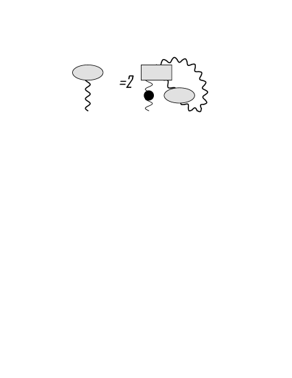
a)            b)

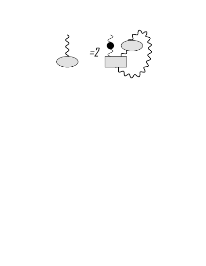
Figure 1: The diagrams a) and b) represent Eq. (A.3) and Eq. (A.4). There are correlators $<B_{\pm}^{a_{1}}\cdots>$, vertices $K^{a_{1}\cdots\,a_{n}}_{b_{1}\cdots b_{m}}$ and bare propagator of the Reggeon fields $G_{0\,-}^{\,bc\,+}$, introduced in Eq. (B.4), denoted by ellipse, rectangle and point figures correspondingly in this and following diagrams.

Now, using Eq. (B.4)-Eq. (B.5) expressions, we will get for the leading contributions to the quantum Reggeon fields:

$$<{\cal B}_{-}^{\,a}>\, = \,2\,G_{0\,-}^{\,a\,a_{1}\,+}\,\left(K^{\,a_{1}\,a_{2}}_{\,a_{3}}\right)^{++}_{-}\,<{\cal B}_{+}^{a_{2}}{\cal B}_{-}^{a_{3}}>\,=\,$$ (A.3)

$$= \,-\,2\,\imath\,G_{0\,-}^{\,a\,a_{1}\,+}\,\left(K^{\,a_{1}\,a_{2}}_{\,a_{3}}\right)^{++}_{-}\,G_{0\,-}^{\,a_{2}\,a_{3}\,+}\,+2\,G_{0\,-}^{\,a\,a_{1}\,+}\,\left(K^{\,a_{1}\,a_{2}}_{\,a_{3}}\right)^{++}_{-}\,<{\cal B}_{+}^{a_{2}}{\cal B}_{-}^{a_{3}}>_{1}\,=\,$$

$$= \,-\,2\,\imath\,G_{0\,-}^{\,a\,a_{1}\,+}\,\left(K^{\,a_{1}\,a_{2}}_{\,a_{2}}\right)^{++}_{-}\,G_{0}^{-+}\,+\,2\,G_{0\,-}^{\,a\,a_{1}\,+}\,\left(K^{\,a_{1}\,a_{2}}_{\,a_{3}}\right)^{++}_{-}\,<{\cal B}_{+}^{a_{2}}{\cal B}_{-}^{a_{3}}>_{1}\,$$

and

$$<{\cal B}_{+}^{\,a}>\, = 2\,G_{0\,-}^{\,a\,a_{1}\,+}\,\left(K^{\,a_{2}}_{\,a_{1}\,a_{3}}\right)^{+}_{--}\,<{\cal B}_{+}^{a_{2}}{\cal B}_{-}^{a_{3}}>\,=\,$$ (A.4)

$$= \,-\,2\,\imath\,G_{0\,-}^{\,a\,a_{1}\,+}\,\left(K^{\,a_{2}}_{\,a_{1}\,a_{3}}\right)^{+}_{--}\,G_{0\,-}^{\,a_{2}\,a_{3}\,+}\,+2\,G_{0\,-}^{\,a\,a_{1}\,+}\,\left(K^{\,a_{2}}_{\,a_{1}\,a_{3}}\right)^{+}_{--}\,<{\cal B}_{+}^{a_{2}}{\cal B}_{-}^{a_{3}}>_{1}\,=\,$$

$$= \,-\,2\,\imath\,G_{0\,-}^{\,a\,a_{1}\,+}\,\left(K^{\,a_{2}}_{\,a_{1}\,a_{2}}\right)^{+}_{--}\,G_{0}^{-+}\,+\,2\,G_{0\,-}^{\,a\,a_{1}\,+}\,\left(K^{\,a_{2}}_{\,a_{1}\,a_{3}}\right)^{+}_{--}\,<{\cal B}_{+}^{a_{2}}{\cal B}_{-}^{a_{3}}>_{1}\,.$$

These expressions contain tadpole contributions built from the Reggeon propagator, which is not enhanced due the presence of the rapidity ordering of the Reggeon fields in the propagator, see [1, 3]. Additionally, to leading order, these effective vertices are proportional to $f_{abc}$ anti-symmetrical structure constant, therefore further we take:

$$<{\cal B}_{-}^{\,a}>\,\approx\,0\,$$ (A.5)

and

$$<{\cal B}_{+}^{\,a}>\,\approx\,0\,,$$ (A.6)

that corresponds to the signature conservation law as well. We also note, that the coefficient $2$ in the front of Eq. (A.3)-Eq. (A.4) arises due the fact we do not symmetrize the expressions in respect to $a_{1}$ and $a_{2}$ indexes. We will keep these form of the shorthand notations further in all the places where it will not lead to any confusion and will write the precise symmetric expressions in respect to the indexes where it will be important.

Appendix B: Correlators of two Reggeon fields

The $<{\cal B}_{+}^{\,a}\,{\cal B}_{-}^{\,a_{1}}>$ correlator of the Reggeon fields is corresponding to the propagator of the reggeized gluons, whereas $<{\cal B}_{+}^{\,a}\,{\cal B}_{+}^{\,a_{1}}>$ and $<{\cal B}_{-}^{\,a}\,{\cal B}_{-}^{\,a_{1}}>$ correlators are suppressed perturbatively in comparison to the first one and represent some kind of the ”mass” terms of the Reggeon fields. Therefore, in the expression for the last two propagators only the first terms will be presented. We have for the correlators of these fields:

$$\partial^{2}_{\bot}\,<{\cal B}_{-}^{\,a}\,{\cal B}_{-}^{\,a_{1}}>\,=\,\left(K^{\,a}_{\,a_{2}}\right)^{+}_{-}\,<{\cal B}_{-}^{\,a_{2}}\,{\cal B}_{-}^{\,a_{1}}>\,+\,2\,\left(K^{\,a\,a_{2}}\right)^{++}\,<{\cal B}_{+}^{\,a_{2}}\,{\cal B}_{-}^{\,a_{1}}>\,+\,\cdot\,$$ (B.1)

and correspondingly

$$\partial^{2}_{\bot}\,<{\cal B}_{+}^{\,a}\,{\cal B}_{+}^{\,a_{1}}>\,=\,\left(K_{a}^{\,a_{2}}\right)^{+}_{-}\,<{\cal B}_{+}^{a_{2}}\,{\cal B}_{+}^{a_{1}}>\,+\,2\,\left(K_{a\,a_{2}}\right)_{--}\,<{\cal B}_{-}^{a_{2}}\,{\cal B}_{+}^{a_{1}}>\,+\,\cdots\,.$$ (B.2)

For the correlator of $\pm$ Reggeon fields we obtain:

$$\partial^{2}_{\bot}\,<{\cal B}_{+}^{\,a}\,{\cal B}_{-}^{\,a_{1}}>\,=\,-\,\imath\,\delta^{\,aa_{1}}\,+\,\left(K_{\,a}^{\,a_{2}}\right)^{+}_{-}\,<{\cal B}_{+}^{\,a_{2}}\,{\cal B}_{-}^{\,a_{1}}>\,+\,2\,\left(K_{a\,a_{2}}\right)_{--}\,<{\cal B}_{-}^{\,a_{2}}\,{\cal B}_{-}^{\,a_{1}}>\,+\,$$ (B.3)

$$+ \,\left(K^{\,a_{2}\,a_{3}}_{a}\right)^{++}_{-}\,<{\cal B}_{+}^{\,a_{3}}\,{\cal B}_{+}^{a_{2}}\,{\cal B}_{-}^{a_{1}}>\,+\,2\,\left(K^{\,a_{2}}_{a\,a_{3}}\right)^{+\,}_{--}\,<{\cal B}_{+}^{\,a_{2}}\,{\cal B}_{-}^{a_{3}}\,{\cal B}_{-}^{a_{1}}>\,+\,$$

$$+ \,3\,\left(K_{a\,a_{2}\,a_{3}}\right)_{---}\,<{\cal B}_{-}^{\,a_{3}}\,{\cal B}_{-}^{a_{2}}\,{\cal B}_{-}^{a_{1}}>\,+\,\left(K_{a}^{\,a_{2}\,a_{3}\,a_{4}}\right)_{-}^{+++}\,<{\cal B}_{+}^{\,a_{2}}\,{\cal B}_{+}^{a_{3}}\,{\cal B}_{+}^{a_{4}}\,{\cal B}_{-}^{\,a_{1}}>\,+\,$$

$$+ \,2\,\left(K_{a\,a_{2}}^{\,a_{3}\,a_{4}}\right)_{--}^{++}\,<{\cal B}_{+}^{\,a_{3}}\,{\cal B}_{+}^{a_{4}}\,{\cal B}_{-}^{a_{2}}\,{\cal B}_{-}^{\,a_{1}}>\,+\,3\,\left(K_{a\,a_{2}\,a_{3}}^{\,a_{4}}\right)_{---}^{+}\,<{\cal B}_{+}^{\,a_{4}}\,{\cal B}_{-}^{a_{3}}\,{\cal B}_{-}^{a_{2}}\,{\cal B}_{-}^{\,a_{1}}>\,+\,$$

$$+ \,4\,\left(K_{a\,a_{2}\,a_{3}\,a_{4}}\right)_{----}\,<{\cal B}_{-}^{\,a_{4}}\,{\cal B}_{-}^{a_{3}}\,{\cal B}_{-}^{a_{2}}\,{\cal B}_{-}^{\,a_{1}}>\,+\,\cdots\,.$$

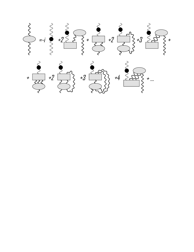
Figure 2: The diagram represents Eq. (B.3). It denotes equation for $<{\cal B}_{+}^{\,a}\,{\cal B}_{-}^{\,a_{1}}>$ correlator.

Now we can introduce the ”bare” propagator of the Reggeon fields as

$$\left(\,\delta^{a\,b}\partial^{2}_{\bot}\,-\,\left(K^{\,a}_{\,b}\right)^{+}_{-}\,\right)\,G_{0\,-}^{\,bc\,+}\,=\,\delta^{a\,c}$$ (B.4)

and obtain the following perturbative expression for the correlator:

$$<{\cal B}_{+}^{\,a}{\cal B}_{-}^{\,b}>=<{\cal B}_{+}^{\,a}{\cal B}_{-}^{\,b}>_{0}+<{\cal B}_{+}^{\,a}{\cal B}_{-}^{\,b}>_{1}=-\imath G_{0\,-}^{\,ab\,+}+<{\cal B}_{+}^{\,a}{\cal B}_{-}^{\,b}>_{1}=-\imath\,\delta^{ab}G_{0}^{+-}+<{\cal B}_{+}^{\,a}\,{\cal B}_{-}^{\,b}>_{1}\,$$ (B.5)

with

$$<{\cal B}_{+}^{\,a}\,{\cal B}_{-}^{\,b}>_{1}\,\propto\,\delta^{\,ab}$$ (B.6)

as well. Therefore, we have for the leading contributions to the r.h.s. of Eq. (B.1) and Eq. (B.2):

$$<{\cal B}_{-}^{\,a}\,{\cal B}_{-}^{\,b}>\, = \,2\,G_{0\,-}^{\,aa_{1}\,+}\,\left(K^{\,a_{1}\,a_{2}}\right)^{++}\,<{\cal B}_{+}^{a_{2}}{\cal B}_{-}^{b}>\,=\,$$

$$- \,2\,\imath\,G_{0\,-}^{\,aa_{1}\,+}\,\left(K^{\,a_{1}\,a_{2}}\right)^{++}\,G_{0\,-}^{\,a_{2}b\,+}\,+\,2\,G_{0\,-}^{\,aa_{1}\,+}\,\left(K^{\,a_{1}\,a_{2}}\right)^{++}\,<{\cal B}_{+}^{a_{2}}{\cal B}_{-}^{b}>_{1}$$ (B.7)

and

$$<{\cal B}_{+}^{\,a}\,{\cal B}_{+}^{\,b}>\, = \,2\,G_{0\,-}^{\,aa_{1}\,+}\,\left(K_{\,a_{1}\,a_{2}}\right)_{--}\,<{\cal B}_{+}^{b}{\cal B}_{-}^{a_{2}}>=\,$$ (B.8)

$$- \,2\,\imath\,G_{0\,-}^{\,aa_{1}\,+}\,\left(K_{\,a_{1}\,a_{2}}\right)_{--}\,G_{0\,-}^{\,ba_{2}\,+}\,+\,2\,G_{0\,-}^{\,aa_{1}\,+}\,\left(K_{\,a_{1}\,a_{2}}\right)_{--}\,<{\cal B}_{+}^{b}{\cal B}_{-}^{a_{2}}>_{1}\,.$$

Now, using Eq. (B.4), Eq. (B.3) reads as:

$$<{\cal B}_{+}^{\,a}\,{\cal B}_{-}^{\,a_{1}}>_{1}\,=\,2\,G_{0\,-}^{\,ab\,+}\,\left(K_{b\,b_{1}}\right)_{--}\,<{\cal B}_{-}^{\,b_{1}}\,{\cal B}_{-}^{\,a_{1}}>\,+\,G_{0\,-}^{\,ab\,+}\,\left(K^{\,b_{1}\,b_{2}}_{b}\right)^{++}_{-}\,<{\cal B}_{+}^{\,b_{1}}\,{\cal B}_{+}^{b_{2}}\,{\cal B}_{-}^{a_{1}}>\,+\,$$ (B.9)

$$+ \,2\,G_{0\,-}^{\,ab\,+}\,\left(K^{\,b_{1}}_{b\,b_{2}}\right)^{+\,}_{--}\,<{\cal B}_{+}^{\,b_{1}}\,{\cal B}_{-}^{b_{2}}\,{\cal B}_{-}^{a_{1}}>\,+\,3\,G_{0\,-}^{\,ab\,+}\,\left(K_{b\,b_{1}\,b_{2}}\right)_{---}\,<{\cal B}_{-}^{\,b_{1}}\,{\cal B}_{-}^{b_{2}}\,{\cal B}_{-}^{a_{1}}>\,+\,$$

$$+ \,2\,G_{0\,-}^{\,ab\,+}\,\left(K_{b\,b_{1}}^{\,b_{2}\,b_{3}}\right)_{--}^{++}\,<{\cal B}_{+}^{\,b_{2}}\,{\cal B}_{+}^{b_{3}}\,{\cal B}_{-}^{b_{1}}\,{\cal B}_{-}^{\,a_{1}}>\,.$$

Inserting LO values of Eq. (Appendix B: Correlators of two Reggeon fields), Eq. (C.7)-Eq. (C.8) and Eq. (D.3) expressions back into the Eq. (B.3), we obtain the following NLO correction to the LO answer for the two Reggeon fields correlator:

$$<{\cal B}_{+}^{\,a}\,{\cal B}_{-}^{\,a_{1}}>_{1}\, = \,-\,4\,\imath\,G_{0\,-}^{\,ab\,+}\,\left(K_{b\,b_{1}}\right)_{--}\,G_{0\,-}^{\,b_{1}b_{2}\,+}\,\left(K^{\,b_{2}\,b_{3}}\right)^{++}\,G_{0\,-}^{\,b_{3}a_{1}\,+}\,-\,$$ (B.10)

$$- \,4\,G_{0\,-}^{\,ab\,+}\,\left(K^{\,b_{1}\,b_{2}}_{b}\right)^{++}_{-}\,G_{0\,-}^{\,b_{1}a_{1}\,+}\,G_{0\,-}^{\,b_{2}b_{3}\,+}\,\left(K^{\,b_{5}}_{\,b_{3}\,b_{4}}\right)^{+}_{--}\,G_{0\,-}^{\,b_{5}b_{4}\,+}\,-$$

$$- \,6\,G_{0\,-}^{\,ab\,+}\,\left(K^{\,b_{1}\,b_{2}}_{b}\right)^{++}_{-}\,G_{0\,-}^{\,b_{4}b_{2}\,+}\,G_{0\,-}^{\,b_{1}b_{3}\,+}\,\left(K^{\,b_{5}}_{b_{3}\,b_{4}}\right)^{+}_{--}\,G_{0\,-}^{\,b_{5}a_{1}\,+}\,-\,$$

$$- 4\,G_{0\,-}^{\,ab\,+}\,\left(K^{\,b_{1}}_{b\,b_{2}}\right)^{+\,}_{--}\,G_{0\,-}^{\,b_{1}b_{2}\,+}\,G_{0\,-}^{\,a_{1}b_{3}\,+}\,\left(K^{\,b_{3}\,b_{4}}_{b_{5}}\right)^{++}_{-}\,G_{0\,-}^{\,b_{4}b_{5}\,+}-\,$$

$$- 4\,G_{0\,-}^{\,ab\,+}\,\left(K^{\,b_{1}}_{b\,b_{2}}\right)^{+\,}_{--}\,G_{0\,-}^{\,b_{1}a_{1}\,+}\,G_{0\,-}^{\,b_{2}b_{3}\,+}\,\left(K^{\,b_{3}\,b_{4}}_{b_{5}}\right)^{++}_{-}\,G_{0\,-}^{\,b_{4}b_{5}\,+}\,-\,$$

$$- 18\,G_{0\,-}^{\,ab\,+}\,\left(K_{b\,b_{1}\,b_{2}}\right)_{---}\,G_{0\,-}^{\,b_{3}b_{1}\,+}\,G_{0\,-}^{\,b_{5}b_{2}\,+}\,\left(K^{\,b_{3}\,b_{4}\,b_{5}}\right)^{+++}\,G_{0\,-}^{\,b_{4}a_{1}\,+}\,\,-\,$$

$$- 4\,G_{0\,-}^{\,ab\,+}\,\left(K_{b\,b_{1}}^{\,b_{2}\,b_{3}}\right)_{--}^{++}\,G_{0\,-}^{\,b_{2}b_{1}\,+}\,G_{0\,-}^{\,b_{3}a_{1}\,+}\,.$$

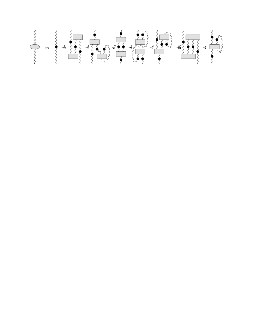
Figure 3: The diagram represents Eq. (B.10). It denotes perturbative solution for $<{\cal B}_{+}^{\,a}\,{\cal B}_{-}^{\,a_{1}}>$ correlator.

Comparing the different contributions in the r.h.s. of the expression we see that the main contribution to the correlator comes from the last term in r.h.s. of Eq. (B.10).

Appendix C: Correlators of three Reggeon fields

There are the following correlators of the three Reggeon fields which we have to calculate, the first one is the following.

$$\partial^{2}_{\bot}\,<\,{\cal B}_{+}^{\,a}{\cal B}_{+}^{\,a_{1}}{\cal B}_{-}^{\,a_{2}}\,>\,=\,-\,\imath\,\delta^{\,aa_{2}}\,<{\cal B}_{+}^{\,a_{1}}>\,+\,\left(K^{\,a_{3}}_{a}\right)^{+}_{-}<\,{\cal B}_{+}^{\,a_{3}}{\cal B}_{+}^{\,a_{1}}{\cal B}_{-}^{\,a_{2}}\,>\,+\,$$ (C.1)

$$+ 2\,\left(K_{aa_{3}}\right)_{--}<\,{\cal B}_{-}^{\,a_{3}}{\cal B}_{+}^{\,a_{1}}{\cal B}_{-}^{\,a_{2}}\,>\,+\left(K^{\,a_{3}a_{4}}_{a}\right)^{++}_{-}<\,{\cal B}_{+}^{\,a_{3}}{\cal B}_{+}^{a_{4}}{\cal B}_{+}^{\,a_{1}}{\cal B}_{-}^{\,a_{2}}\,>+$$

$$+ 2\left(K^{\,a_{4}}_{aa_{3}}\right)^{+}_{--}<\,{\cal B}_{+}^{\,a_{4}}{\cal B}_{-}^{a_{3}}{\cal B}_{+}^{\,a_{1}}{\cal B}_{-}^{\,a_{2}}\,>+3\left(K_{aa_{3}a_{4}}\right)_{---}<\,{\cal B}_{-}^{\,a_{3}}{\cal B}_{-}^{a_{4}}{\cal B}_{+}^{\,a_{1}}{\cal B}_{-}^{\,a_{2}}\,>\,.$$

The second one can be obtained from the first one by replace $+$ on $-$ in the expression:

$$\partial^{2}_{\bot}\,<\,{\cal B}_{-}^{\,a}{\cal B}_{-}^{\,a_{1}}{\cal B}_{+}^{\,a_{2}}\,>\,=\,-\,2\imath\,\delta^{\,aa_{2}}\,<{\cal B}_{-}^{\,a_{1}}>\,+\,\left(K^{\,a}_{a_{3}}\right)^{+}_{-}<\,{\cal B}_{-}^{\,a_{3}}{\cal B}_{+}^{\,a_{1}}{\cal B}_{+}^{\,a_{2}}\,>\,+\,$$ (C.2)

$$+ 2\,\left(K^{aa_{3}}\right)^{++}<\,{\cal B}_{+}^{\,a_{3}}{\cal B}_{-}^{\,a_{1}}{\cal B}_{+}^{\,a_{2}}\,>\,+\left(K_{\,a_{3}a_{4}}^{a}\right)^{+}_{--}<\,{\cal B}_{-}^{\,a_{3}}{\cal B}_{-}^{a_{4}}{\cal B}_{-}^{\,a_{1}}{\cal B}_{+}^{\,a_{2}}\,>+$$

$$+ 2\left(K_{\,a_{4}}^{\,aa_{3}}\right)^{++}_{-}<\,{\cal B}_{-}^{\,a_{4}}{\cal B}_{+}^{a_{3}}{\cal B}_{-}^{\,a_{1}}{\cal B}_{+}^{\,a_{2}}\,>+3\left(K^{\,aa_{3}a_{4}}\right)^{+++}<\,{\cal B}_{+}^{\,a_{3}}{\cal B}_{+}^{a_{4}}{\cal B}_{-}^{\,a_{1}}{\cal B}_{+}^{\,a_{2}}\,>\,$$

and the third one:

$$\partial^{2}_{\bot}\,<\,{\cal B}_{-}^{\,a}{\cal B}_{-}^{\,a_{1}}{\cal B}_{-}^{\,a_{2}}\,>\,=\,\left(K_{a_{3}}^{\,a}\right)^{+}_{-}<\,{\cal B}_{-}^{\,a_{3}}{\cal B}_{-}^{\,a_{1}}{\cal B}_{-}^{\,a_{2}}\,>\,+\,2\left(K^{\,aa_{3}}\right)^{+}_{-}<\,{\cal B}_{+}^{\,a_{3}}{\cal B}_{-}^{\,a_{1}}{\cal B}_{-}^{\,a_{2}}\,>\,+\,$$ (C.3)

$$+ \left(K^{\,a}_{a_{3}a_{4}}\right)^{+}_{--}<\,{\cal B}_{-}^{\,a_{3}}{\cal B}_{-}^{a_{4}}{\cal B}_{-}^{\,a_{1}}{\cal B}_{-}^{\,a_{2}}\,>\,+\,2\left(K^{\,aa_{3}}_{a_{4}}\right)^{++}_{-}<\,{\cal B}_{+}^{\,a_{3}}{\cal B}_{-}^{a_{4}}{\cal B}_{-}^{\,a_{1}}{\cal B}_{-}^{\,a_{2}}\,>\,+\,$$

$$+ 3\left(K^{\,aa_{3}a_{4}}\right)^{+++}<\,{\cal B}_{+}^{\,a_{3}}{\cal B}_{+}^{a_{4}}{\cal B}_{-}^{\,a_{1}}{\cal B}_{-}^{\,a_{2}}\,>\,.$$

This system of equations can be solved perturbatively, using results of the Appendix A and Appendix D, here we will use the symmetric expression for Eq. (D.3):

$$<\,{\cal B}_{+}^{\,a}{\cal B}_{+}^{\,a_{1}}{\cal B}_{-}^{\,a_{2}}{\cal B}_{-}^{\,a_{3}}\,>\, = \,-\,G_{0\,-}^{\,aa_{3}\,+}\,G_{0\,-}^{\,a_{1}a_{2}\,+}\,-\,G_{0\,-}^{\,aa_{2}\,+}\,G_{0\,-}^{\,a_{1}a_{3}\,+}\,-\,$$ (C.4)

$$- \,\imath\,G_{0\,-}^{\,aa_{3}\,+}\,<\,{\cal B}_{+}^{\,a_{1}}{\cal B}_{-}^{a_{2}}\,>_{1}\,-\,\imath\,G_{0\,-}^{\,a_{1}\,a_{2}\,+}\,<\,{\cal B}_{+}^{\,a}{\cal B}_{-}^{a_{3}}\,>_{1}\,.$$

We obtain for Eq. (C.3):

$$<\,{\cal B}_{-}^{\,a}{\cal B}_{-}^{\,a_{1}}{\cal B}_{-}^{\,a_{2}}\,>\,=\,2\,G_{0\,-}^{\,ab\,+}\,\left(K^{\,bb_{1}}\right)^{+}_{-}<\,{\cal B}_{+}^{\,b_{1}}{\cal B}_{-}^{\,a_{1}}{\cal B}_{-}^{\,a_{2}}\,>\,-\,$$ (C.5)

$$- 6\,G_{0\,-}^{\,a{\cal B}_{2}\,+}\,\left(K^{\,b_{2}b_{3}b_{4}}\right)^{+++}\Big{(}G_{0\,-}^{\,b_{3}a_{2}\,+}\,G_{0\,-}^{\,b_{4}a_{1}\,+}+\imath\,G_{0\,-}^{\,b_{3}a_{2}\,+}\,<\,{\cal B}_{+}^{\,b_{4}}{\cal B}_{-}^{a_{1}}\,>_{1}\Big{)}\,,$$

that to leading order gives

$$<\,{\cal B}_{-}^{\,a}{\cal B}_{-}^{\,a_{1}}{\cal B}_{-}^{\,a_{2}}\,>\, = \,-\,6\imath\,G_{0\,-}^{\,b_{1}a_{2}\,+}\,\left(K^{\,bb_{1}b_{2}}\right)^{+++}\,G_{0\,-}^{\,b_{1}a_{2}\,+}\,<\,{\cal B}_{+}^{\,b_{2}}{\cal B}_{-}^{\,a_{1}}\,>\,=\,$$ (C.6)

$$= -6\,G_{0\,-}^{\,ab\,+}\,\left(K^{\,bb_{1}b_{2}}\right)^{+++}\Big{(}G_{0\,-}^{\,b_{1}a_{2}\,+}\,G_{0\,-}^{\,b_{2}a_{1}\,+}+\imath G_{0\,-}^{\,b_{1}a_{2}\,+}\,<\,{\cal B}_{+}^{\,b_{2}}{\cal B}_{-}^{\,a_{1}}\,>_{1}\Big{)}.$$

Correspondingly, for Eq. (C.1) we have to the leading order:

$$<\,{\cal B}_{+}^{\,a}{\cal B}_{+}^{\,a_{1}}{\cal B}_{-}^{\,a_{2}}\,>\,=\,-\,\imath\,G_{0\,-}^{\,aa_{2}\,+}\,\,<{\cal B}_{+}^{\,a_{1}}>\,+\,2\,G_{0\,-}^{\,ab\,+}\,\left(K^{\,b_{1}}_{bb_{2}}\right)^{+}_{--}<\,{\cal B}_{+}^{\,b_{1}}{\cal B}_{+}^{\,a_{1}}{\cal B}_{-}^{\,a_{2}}{\cal B}_{-}^{b_{2}}\,>\,=$$ (C.7)

$$= \,-\,2\,\imath\,G_{0\,-}^{\,aa_{2}\,+}\,G_{0\,-}^{\,a_{1}\,b\,+}\,\left(K^{\,b_{1}}_{b\,\,b_{2}}\right)^{+}_{--}\,<{\cal B}_{+}^{b_{1}}{\cal B}_{-}^{b_{2}}>\,-\,2\imath\,G_{0\,-}^{\,a_{1}\,b\,+}\,\left(K^{\,b_{1}}_{b\,\,b_{2}}\right)^{+}_{--}\,G_{0\,-}^{\,b_{1}b_{2}\,+}\,<{\cal B}_{+}^{a}{\cal B}_{-}^{a_{2}}>\,-$$

$$- \imath\,G_{0\,-}^{\,ab\,+}\,\left(K^{\,b_{1}}_{b\,b_{2}}\right)^{+}_{--}G_{0\,-}^{\,b_{1}a_{2}\,+}\,<{\cal B}_{+}^{\,a_{1}}{\cal B}_{-}^{\,b_{2}}>\,-\imath\,G_{0\,-}^{\,ab\,+}\,\left(K^{\,b_{1}}_{b\,b_{2}}\right)^{+}_{--}G_{0\,-}^{\,b_{2}a_{2}\,+}\,<{\cal B}_{+}^{\,b_{1}}{\cal B}_{-}^{\,a_{1}}>=$$

$$= \,\,-4\,G_{0\,-}^{\,aa_{2}\,+}\,G_{0\,-}^{\,a_{1}\,b\,+}\,\left(K^{\,b_{1}}_{b\,\,b_{2}}\right)^{+}_{--}\,G_{0\,-}^{\,b_{1}\,b_{2}\,+}\,-\,2\,\imath\,G_{0\,-}^{\,aa_{2}\,+}\,G_{0\,-}^{\,a_{1}\,b\,+}\,\left(K^{\,b_{1}}_{b\,\,b_{2}}\right)^{+}_{--}\,<{\cal B}_{+}^{b_{1}}{\cal B}_{-}^{b_{2}}>_{1}\,-$$

$$- 2\,G_{0\,-}^{\,ab\,+}\,\left(K^{\,b_{2}}_{b\,b_{1}}\right)^{+}_{--}\,G_{0\,-}^{\,a_{1}b_{1}\,+}\,G_{0\,-}^{\,b_{2}a_{2}\,+}\,-\,\,2\imath\,G_{0\,-}^{\,a_{1}\,b\,+}\,\left(K^{\,b_{1}}_{b\,\,b_{2}}\right)^{+}_{--}\,G_{0\,-}^{\,b_{1}b_{2}\,+}\,<{\cal B}_{+}^{a}{\cal B}_{-}^{a_{2}}>_{1}-$$

$$- \imath\,G_{0\,-}^{\,ab\,+}\,\left(K^{\,b_{1}}_{b\,b_{2}}\right)^{+}_{--}G_{0\,-}^{\,b_{1}a_{2}\,+}\,<{\cal B}_{+}^{\,a_{1}}{\cal B}_{-}^{\,b_{2}}>_{1}-\imath\,G_{0\,-}^{\,ab\,+}\,\left(K^{\,b_{1}}_{b\,b_{2}}\right)^{+}_{--}G_{0\,-}^{\,b_{2}a_{1}\,+}\,<{\cal B}_{+}^{\,b_{1}}{\cal B}_{-}^{\,a_{2}}>_{1}\,,$$

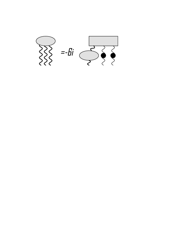
Figure 4: The represents Eq. (C.5). It denotes LO expression of $<\,{\cal B}_{-}^{\,a}{\cal B}_{-}^{\,a_{1}}{\cal B}_{-}^{\,a_{2}}\,>$ correlator in terms of Reggeon propagator.

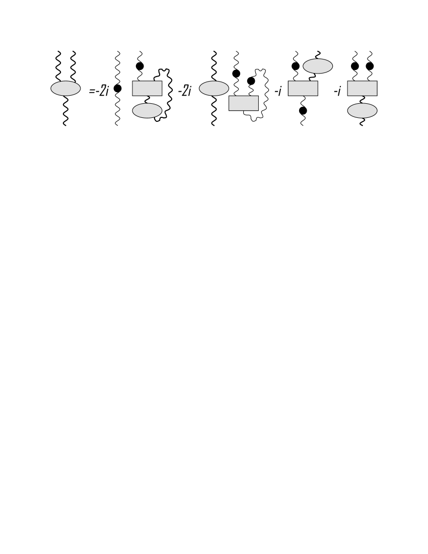
Figure 5: The represents Eq. (C.7). It denotes LO expression of $<\,{\cal B}_{+}^{\,a}{\cal B}_{+}^{\,a_{1}}{\cal B}_{-}^{\,a_{2}}\,>$ correlator in terms of Reggeon propagator.

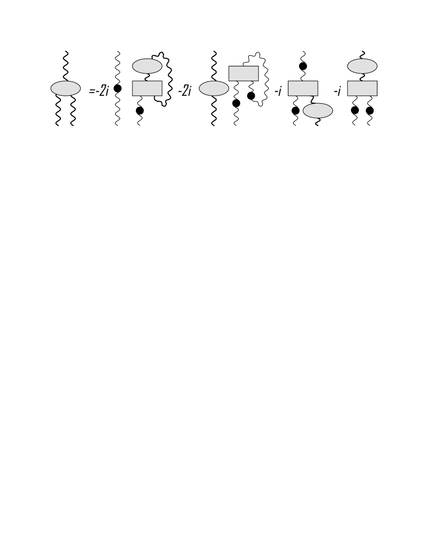
Figure 6: The diagram represents Eq. (C.8). It denotes LO expression of $<\,{\cal B}_{+}^{\,a}{\cal B}_{-}^{\,a_{1}}{\cal B}_{-}^{\,a_{2}}\,>$ correlator in terms of Reggeon propagator.

we note, that we wrote Eq. (C.7) in the mostly symmetrical way. Correspondingly, the answer for Eq. (C.2) can be obtained from Eq. (C.7) by replace of the $+$ and $-$ signs in Eq. (C.7):

$$<\,{\cal B}_{+}^{\,a}{\cal B}_{-}^{\,a_{1}}{\cal B}_{-}^{\,a_{2}}\,>\,=\,-\,2\imath\,G_{0\,-}^{\,aa_{1}\,+}\,<{\cal B}_{-}^{\,a_{2}}>\,+\,G_{0\,-}^{\,ab\,+}\,\left(K^{\,b_{1}b_{2}}_{b}\right)^{++}_{-}<\,{\cal B}_{+}^{\,b_{1}}{\cal B}_{+}^{\,b_{2}}{\cal B}_{-}^{\,a_{1}}{\cal B}_{-}^{\,a_{2}}\,>\,=$$ (C.8)

$$= \,\,-\,2\,\imath\,G_{0\,-}^{\,aa_{1}\,+}\,G_{0\,-}^{\,a_{2}\,b\,+}\,\left(K^{\,b\,b_{1}}_{\,b_{2}}\right)^{++}_{-}\,<{\cal B}_{+}^{b_{1}}{\cal B}_{-}^{b_{2}}>\,-2\,\imath\,G_{0\,-}^{\,a_{2}\,b\,+}\,\left(K^{\,b\,b_{1}}_{\,b_{2}}\right)^{++}_{-}\,G_{0\,-}^{\,b_{1}b_{2}\,+}\,<{\cal B}_{+}^{a}{\cal B}_{-}^{a_{1}}>\,-\,$$

$$- \imath\,G_{0\,-}^{\,ab\,+}\,\left(K^{\,b_{1}b_{2}}_{b}\right)^{++}_{-}\,G_{0\,-}^{\,b_{1}a_{2}\,+}\,<\,{\cal B}_{+}^{\,b_{2}}{\cal B}_{-}^{\,a_{1}}\,>\,-\,\imath\,G_{0\,-}^{\,b_{1}a_{1}\,+}\,\left(K^{\,b_{1}b_{2}}_{b}\right)^{++}_{-}\,G_{0\,-}^{\,b_{2}a_{2}\,+}\,<\,{\cal B}_{+}^{\,a}{\cal B}_{-}^{\,b}\,>=$$

$$= \,-4\,G_{0\,-}^{\,aa_{1}\,+}\,G_{0\,-}^{\,a_{2}\,b\,+}\,\left(K^{\,b\,b_{1}}_{\,b_{2}}\right)^{++}_{-}\,G_{0\,-}^{\,b_{1}\,b_{2}\,+}\,-\,2\,\imath\,G_{0\,-}^{\,aa_{1}\,+}\,G_{0\,-}^{\,a_{2}\,b\,+}\,\left(K^{\,b\,b_{1}}_{\,b_{2}}\right)^{++}_{-}\,<{\cal B}_{+}^{b_{1}}{\cal B}_{-}^{b_{2}}>_{1}\,-$$

$$- \,2\,G_{0\,-}^{\,ab\,+}\,\left(K^{\,b_{1}b_{2}}_{b}\right)^{++}_{-}\,G_{0\,-}^{\,b_{1}a_{2}\,+}\,G_{0\,-}^{\,b_{2}a_{1}\,+}\,-2\,\imath\,G_{0\,-}^{\,a_{2}\,b\,+}\,\left(K^{\,b\,b_{1}}_{\,b_{2}}\right)^{++}_{-}\,G_{0\,-}^{\,b_{1}b_{2}\,+}\,<{\cal B}_{+}^{a}{\cal B}_{-}^{a_{1}}>_{1}\,-\,$$

$$- 2\,\imath\,G_{0\,-}^{\,ab\,+}\,\left(K^{\,b_{1}b_{2}}_{b}\right)^{++}_{-}\,G_{0\,-}^{\,b_{1}a_{2}\,+}\,<\,{\cal B}_{+}^{\,b_{2}}{\cal B}_{-}^{\,a_{1}}\,>_{1}\,,$$

that can be verified by the direct calculation of Eq. (C.2).

Appendix D: Correlators of four Reggeon fields

We limit the chain of the equations by the 4-Reggeon correlators, therefore the equations for these correlators are simple. We have for the symmetrical correlator of four Reggeon fields:

$$\partial^{2}_{\bot}\,<\,{\cal B}_{+}^{\,a}{\cal B}_{+}^{\,a_{1}}{\cal B}_{-}^{\,a_{2}}{\cal B}_{-}^{\,a_{3}}\,>\, = \,-\,2\,\imath\,\delta^{\,aa_{3}}\,<\,{\cal B}_{+}^{\,a_{1}}{\cal B}_{-}^{a_{2}}\,>\,+\,\left(K^{\,a_{4}}_{a}\right)^{+}_{-}<\,{\cal B}_{+}^{\,a_{4}}{\cal B}_{+}^{\,a_{1}}{\cal B}_{-}^{\,a_{2}}{\cal B}_{-}^{\,a_{3}}\,>\,+$$ (D.1)

$$+ \,2\,\left(K_{aa_{4}}\right)_{--}<\,{\cal B}_{-}^{\,a_{4}}{\cal B}_{+}^{\,a_{1}}{\cal B}_{-}^{\,a_{2}}{\cal B}_{-}^{\,a_{3}}\,>\,,$$

where correspondingly:

$$\partial^{2}_{\bot}\,<\,{\cal B}_{-}^{\,a}{\cal B}_{-}^{\,a_{1}}{\cal B}_{-}^{\,a_{2}}{\cal B}_{+}^{\,a_{3}}\,>\, = \,-\,\imath\,\delta^{\,aa_{3}}\,<\,{\cal B}_{-}^{\,a_{1}}{\cal B}_{-}^{a_{2}}\,>\,+\,\left(K_{\,a_{4}}^{a}\right)^{+}_{-}<\,{\cal B}_{-}^{\,a_{4}}{\cal B}_{-}^{\,a_{1}}{\cal B}_{-}^{\,a_{2}}{\cal B}_{+}^{\,a_{3}}\,>\,+$$ (D.2)

$$+ \,2\,\left(K^{aa_{4}}\right)^{++}\,<\,{\cal B}_{+}^{\,a_{4}}{\cal B}_{-}^{\,a_{1}}{\cal B}_{-}^{\,a_{2}}{\cal B}_{+}^{\,a_{3}}\,>\,.$$

Solving these equations perturbatively and using Eq. (B.5)-Eq. (Appendix B: Correlators of two Reggeon fields) we obtain:

$$<{\cal B}_{+}^{\,a}{\cal B}_{+}^{\,a_{1}}{\cal B}_{-}^{\,a_{2}}{\cal B}_{-}^{\,a_{3}}>=-\,2\,\imath\,G_{0\,-}^{\,aa_{3}\,+}\,<{\cal B}_{+}^{\,a_{1}}{\cal B}_{-}^{a_{2}}>=-2\,G_{0\,-}^{\,aa_{3}\,+}\,G_{0\,-}^{\,a_{1}a_{2}\,+}-2\,\imath\,G_{0\,-}^{\,aa_{3}\,+}\,<{\cal B}_{+}^{\,a_{1}}{\cal B}_{-}^{a_{2}}>_{1}\,,$$ (D.3)

and

$$<{\cal B}_{-}^{\,a}{\cal B}_{-}^{\,a_{1}}{\cal B}_{-}^{\,a_{2}}{\cal B}_{+}^{\,a_{3}}>=-3\imath G_{0\,-}^{\,a_{1}b\,+}\,\left(K^{bb_{1}}\right)^{++}G_{0\,-}^{\,b_{1}a_{2}\,+}<{\cal B}_{+}^{\,a_{3}}{\cal B}_{-}^{a}>-$$ (D.4)

$$- 3\imath G_{0\,-}^{\,a_{1}a_{3}\,+}\,\left(K^{bb_{1}}\right)^{++}G_{0\,-}^{\,b_{1}a_{2}\,+}<{\cal B}_{+}^{\,b}{\cal B}_{-}^{a}>=-6G_{0\,-}^{\,aa_{3}\,+}G_{0\,-}^{\,a_{1}b\,+}\left(K^{bb_{1}}\right)^{++}G_{0\,-}^{\,b_{1}a_{2}\,+}.$$

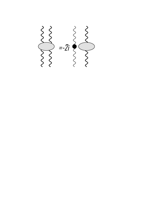
Figure 7: The diagram represents Eq. (D.3). It denotes LO expression of $<{\cal B}_{+}^{\,a}{\cal B}_{+}^{a_{1}}{\cal B}_{-}^{\,a_{2}}{\cal B}_{-}^{\,a_{3}}>$ correlator in terms of Reggeon propagator.

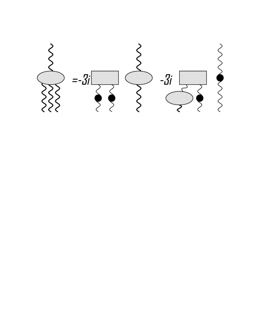
Figure 8: The diagram represents Eq. (D.4). It denotes LO expression of $<{\cal B}_{-}^{\,a}{\cal B}_{-}^{\,a_{1}}{\cal B}_{-}^{\,a_{2}}{\cal B}_{+}^{\,a_{3}}>$ correlator in terms of Reggeon propagator.

We note, that the leading contribution of Eq. (D.4) correlator is to $g^{2}$ order, i.e. a leading order of the $K^{++}$ vertex is $g^{2}$ at least. Corresponding $<{\cal B}_{-}{\cal B}_{-}{\cal B}_{+}{\cal B}_{+}>$ and $<{\cal B}_{+}{\cal B}_{+}{\cal B}_{+}{\cal B}_{-}>$ correlators can be obtained from the Eq. (D.3)-Eq. (D.4) expressions by the change $+$ to $-$ and vise versa in the effective vertices in the expressions.

For the other correlators we correspondingly have:

$$\partial^{2}_{\bot}\,<\,{\cal B}_{+}^{\,a}{\cal B}_{-}^{\,a_{1}}{\cal B}_{-}^{\,a_{2}}{\cal B}_{-}^{\,a_{3}}\,>\, = \,-\,3\,\imath\,\delta^{\,aa_{1}}\,<\,{\cal B}_{-}^{\,a_{2}}{\cal B}_{-}^{a_{3}}\,>\,+\,\left(K^{\,a_{4}}_{\,a}\right)^{+}_{-}<\,{\cal B}_{+}^{\,a_{4}}{\cal B}_{-}^{\,a_{1}}{\cal B}_{-}^{\,a_{2}}{\cal B}_{-}^{\,a_{3}}\,>\,+$$ (D.5)

$$+ \,2\,\left(K_{aa_{4}}\right)_{--}<\,{\cal B}_{-}^{\,a_{4}}{\cal B}_{-}^{\,a_{1}}{\cal B}_{-}^{\,a_{2}}{\cal B}_{-}^{\,a_{3}}\,>\,$$

and

$$\partial^{2}_{\bot}<{\cal B}_{-}^{\,a}{\cal B}_{-}^{\,a_{1}}{\cal B}_{-}^{\,a_{2}}{\cal B}_{-}^{\,a_{3}}>=\left(K_{\,a_{4}}^{\,a}\right)^{+}_{-}<{\cal B}_{-}^{\,a_{4}}{\cal B}_{-}^{\,a_{1}}{\cal B}_{-}^{\,a_{2}}{\cal B}_{-}^{\,a_{3}}>+2\left(K^{\,aa_{4}}\right)^{++}<{\cal B}_{+}^{\,a_{4}}{\cal B}_{-}^{\,a_{1}}{\cal B}_{-}^{\,a_{2}}{\cal B}_{-}^{\,a_{3}}>\,.$$ (D.6)

Solving the system perturbatively, we obtain:

$$<{\cal B}_{-}^{\,a}{\cal B}_{-}^{\,a_{1}}{\cal B}_{-}^{\,a_{2}}{\cal B}_{-}^{\,a_{3}}>\, = 2\,G_{0\,-}^{\,ab\,+}\,\left(K^{\,bb_{1}}\right)^{++}<{\cal B}_{+}^{\,b_{1}}{\cal B}_{-}^{\,a_{1}}{\cal B}_{-}^{\,a_{2}}{\cal B}_{-}^{\,a_{3}}>\,=\,$$

$$= \,-\,12\,\imath\,G_{0\,-}^{\,ab\,+}\,\left(K^{\,bb_{1}}\right)^{++}\,<B_{+}^{b_{1}}B_{-}^{a_{1}}>\,G_{0\,-}^{\,a_{2}c\,+}\,\left(K^{\,cc_{1}}\right)^{++}\,G_{0\,-}^{\,c_{1}a_{3}\,+}\,$$ (D.7)

that provides for the first correlator:

$$<{\cal B}_{+}^{\,a}{\cal B}_{-}^{\,a_{1}}{\cal B}_{-}^{\,a_{2}}{\cal B}_{-}^{\,a_{3}}>=-6\Big{[}\left(\delta-4G_{0\,-}^{\,+}K_{--}G_{0\,-}^{\,+}K^{++}\right)^{\,a}_{b}\Big{]}^{-1}\,G_{0\,-}^{\,ba_{1}\,+}\,G_{0\,-}^{\,a_{2}b_{2}\,+}\,\left(K^{\,b_{2}\,b_{3}}\right)^{++}\,G_{0\,-}^{\,b_{3}a_{3}\,+}\,,$$ (D.8)

or to leading approximation

$$<{\cal B}_{+}^{\,a}{\cal B}_{-}^{\,a_{1}}{\cal B}_{-}^{\,a_{2}}{\cal B}_{-}^{\,a_{3}}>\,=\,-6\,G_{0\,-}^{\,aa_{1}\,+}\,G_{0\,-}^{\,a_{2}b\,+}\,\left(K^{\,b\,b_{1}}\right)^{++}\,G_{0\,-}^{\,b_{1}a_{3}\,+}\,,$$ (D.9)

that precisely reproduce Eq. (D.4) expression. Hence we obtain for Eq. (Appendix D: Correlators of four Reggeon fields):

$$<{\cal B}_{-}^{\,a}{\cal B}_{-}^{\,a_{1}}{\cal B}_{-}^{\,a_{2}}{\cal B}_{-}^{\,a_{3}}>\,=\,-12\,G_{0\,-}^{\,ab\,+}\,\left(K^{\,bb_{1}}\right)^{++}\,G_{0\,-}^{\,b_{1}a_{1}\,+}\,G_{0\,-}^{\,a_{2}b_{2}\,+}\,\left(K^{\,b_{2}\,b_{3}}\right)^{++}\,G_{0\,-}^{\,b_{3}a_{3}\,+}\,.$$ (D.10)

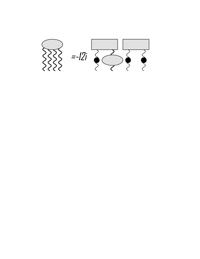
Figure 9: The diagram represents Eq. (D.10). It denotes $<{\cal B}_{-}^{\,a}{\cal B}_{-}^{\,a_{1}}{\cal B}_{-}^{\,a_{2}}{\cal B}_{-}^{\,a_{3}}>\,$ correlator in terms of Reggeon propagator.

References

- [1] L. N. Lipatov, Nucl. Phys. B 452, 369 (1995); Phys. Rept. 286, (1997) 131; Subnucl. Ser. 49,(2013) 131; Int. J. Mod. Phys. Conf. Ser. 39, (2015) 1560082; Int. J. Mod. Phys. A 31, no. 28/29, (2016) 1645011; EPJ Web Conf. 125, (2016) 01010.
- [2] S. Bondarenko, L. Lipatov and A. Prygarin, Eur. Phys. J. C 77 (2017) no.8, 527.
- [3] S. Bondarenko, L. Lipatov, S. Pozdnyakov and A. Prygarin, Eur. Phys. J. C 77 (2017) no. 9, 630.
- [4] S. Bondarenko and S. S. Pozdnyakov, Phys. Lett. B 783 (2018) 207.
- [5] S. Bondarenko and M. A. Zubkov, Eur. Phys. J. C 78 (2018) no.8, 617.
- [6] L. N. Lipatov, Nucl. Phys. Proc. Suppl. 99A, (2001) 175; M. A. Braun and M. I. Vyazovsky, Eur. Phys. J. C 51, (2007) 103; M. A. Braun, M. Y. Salykin and M. I. Vyazovsky, Eur. Phys. J. C 65, (2010) 385; M. A. Braun, L. N. Lipatov, M. Y. Salykin and M. I. Vyazovsky, Eur. Phys. J. C 71, (2011) 1639; M. A. Braun, M. Y. Salykin and M. I. Vyazovsky, Eur. Phys. J. C 72, 1864 (2012); M. Hentschinski and A. Sabio Vera, Phys. Rev. D 85, 056006 (2012); M. A. Braun, M. Y. Salykin, S. S. Pozdnyakov and M. I. Vyazovsky, Eur. Phys. J. C 72, (2012) 2223; J. Bartels, L. N. Lipatov and G. P. Vacca, Phys. Rev. D 86, (2012) 105045; M. A. Braun, S. S. Pozdnyakov, M. Y. Salykin and M. I. Vyazovsky, Eur. Phys. J. C 73, no. 9, (2013) 2572; G. Chachamis, M. Hentschinski, J. D. Madrigal Martínez and A. Sabio Vera, Phys. Part. Nucl. 45, no. 4, (2014) 788; M. A. Braun, Eur. Phys. J. C 75 (2015) no.7, 298; M. A. Braun and M. I. Vyazovsky, Phys. Rev. D 93 (2016) no.6, 065026; M. A. Braun, Eur. Phys. J. C 77 (2017) no.5, 279; M. A. Braun and M. Y. Salykin, Eur. Phys. J. C 77 (2017) no.7, 498.
- [7] L.D. Faddeev, A.A. Slavnov, ”Gauge Fields. Introduction to Quantum Theory”, The Benjamin Cummings Publishing Company, 1980; I.Y.Arefeva, L.D.Faddeev and A.A.Slavnov, Theor. Math. Phys. 21, 1165 (1975) [Teor. Mat. Fiz. 21, 311 (1974)].
- [8] V. N. Gribov, Sov. Phys. JETP 26 (1968) 414.
- [9] L. N. Lipatov, Sov. J. Nucl. Phys. 23, 338 (1976) [Yad. Fiz. 23 (1976) 642]; E. A. Kuraev, L. N. Lipatov and V. S. Fadin, Sov. Phys. JETP 45, 199 (1977) [Zh. Eksp. Teor. Fiz. 72, 377 (1977)]; I. I. Balitsky and L. N. Lipatov, Sov. J. Nucl. Phys. 28, 822 (1978) [Yad. Fiz. 28, 1597 (1978)].
- [10] V. S. Fadin and L. N. Lipatov, Eur. Phys. J. C 78 (2018) no.6, 439.
- [11] J. Bartels, Nucl. Phys. B 175 (1980) 365; J. Kwiecinski, M. Praszalowicz, Phys. Lett. B 94 (1980) 413; J. Bartels, V. S. Fadin, L. N. Lipatov and G. P. Vacca, Nucl. Phys. B 867, (2013) 827.
- [12] L. V. Gribov, E. M. Levin and M. G. Ryskin, Phys.Rep. 100, 1 (1983).
- [13] I. Balitsky, Nucl. Phys. B463 (1996) 99; Y. V. Kovchegov, Phys. Rev. D60 (1999) 034008; Phys. Rev. D61 (2000) 074018; I. Balitsky, Phys. Rev. D 60, 014020 (1999); In *Shifman, M. (ed.): At the frontier of particle physics, vol. 2* 1237-1342; Nucl. Phys. B 629, 290 (2002).
- [14] J. Bartels, Z. Phys. C 60 (1993) 471; J. Bartels and M. W¨usthoff, Z. Phys. C 66 (1995) 157; J. Bartels and C. Ewerz, JHEP 9909 (1999) 026.
- [15] M. Hentschinski, Phys. Rev. D 97 (2018) no.11, 114027.
- [16] L. McLerran and R. Venugopalan, Phys. Rev. D49 (1994), 2233; D49 (1994), 3352.
- [17] J. Jalilian-Marian, A. Kovner, L. McLerran and H. Weigert, Phys.Rev. D55, (1997) 5414; J. Jalilian-Marian, A. Kovner, A. Leonidov and H. Weigert, Nucl. Phys. B 504, (1997) 415; J. Jalilian-Marian, A. Kovner, A. Leonidov and H. Weigert, Phys. Rev. D 59,(1998) 014014 ; E. Iancu, A. Leonidov and L. D. McLerran, Nucl. Phys. A 692, (2001) 583; E. Iancu, A. Leonidov and L. D. McLerran, Phys. Lett. B 510, (2001) 133; E. Ferreiro, E. Iancu, A. Leonidov and L. McLerran, Nucl. Phys. A 703, (2002) 489; K. Roy and R. Venugopalan, arXiv:1802.09550 [hep-ph].
- [18] I. Balitsky, Phys. Rev. D 72, (2005) 074027; Y. Hatta, Nucl. Phys. A 768, (2006) 222; Y. Hatta, E. Iancu, L. McLerran, A. Stasto and D. N. Triantafyllopoulos, Nucl. Phys. A 764,(2006) 423. Y. Hatta, Nucl. Phys. A 781, (2007) 104.
- [19] M. Nefedov and V. Saleev, Mod. Phys. Lett. A 32 (2017) no.40, 1750207; A. V. Karpishkov, M. A. Nefedov, V. A. Saleev and A. V. Shipilova, Phys. Part. Nucl. 48 (2017) no.5, 827 [Fiz. Elem. Chast. Atom. Yadra 48 (2017) no.5 ].
- [20] V. S. Fadin, R. Fiore and A. Papa, Phys. Lett. B 647 (2007) 179; V. S. Fadin, R. Fiore and A. Papa, Nucl. Phys. B 769, (2007) 108; V. S. Fadin, R. Fiore, A. V. Grabovsky and A. Papa, Nucl. Phys. B 784 (2007) 49; V. S. Fadin, AIP Conf. Proc. 1105 (2009) 340.
- [21] V. S. Fadin and R. Fiore, Phys. Lett. B 294 (1992) 286; V. S. Fadin, R. Fiore and A. Quartarolo, Phys. Rev. D 50 (1994) 2265; V. S. Fadin, R. Fiore and A. Quartarolo, Phys. Rev. D 50 (1994) 5893; V. S. Fadin, R. Fiore and M. I. Kotsky, Phys. Lett. B 389 (1996) 737; V. S. Fadin, R. Fiore and A. Papa, Phys. Rev. D 63 (2001) 034001; V. S. Fadin and R. Fiore, Phys. Rev. D 64 (2001) 114012 V. S. Fadin, M. G. Kozlov and A. V. Reznichenko, Phys. Atom. Nucl. 67 (2004) 359 [Yad. Fiz. 67 (2004) 377]; M. G. Kozlov, A. V. Reznichenko and V. S. Fadin, Phys. Atom. Nucl. 75 (2012) 850; V. S. Fadin, arXiv:1507.08756 [hep-th].
- [22] B.L. Ioffe, V.S.Fadin and L.N.Lipatov, ”Quantum chromodynamics”, Cambridge University Press, 2010.
- [23] H. J. De Vega and L. N. Lipatov, Phys. Rev. D 64 (2001) 114019; H. J. de Vega and L. N. Lipatov, Phys. Rev. D 66 (2002) 074013; L. N. Lipatov, Phys. Usp. 47 (2004) 325 [Usp. Fiz. Nauk 47 (2004) 337]; J. Bartels, L. N. Lipatov and A. Prygarin, J. Phys. A 44 (2011) 454013; L. N. Lipatov, AIP Conf. Proc. 1523 (2012) 247.
- [24] S. Bondarenko and A. Prygarin, JHEP 1607 (2016) 081.