PMU Placement Optimization for Smart Grid Obvervability and State Estimation

Abstract

In this paper, phasor measurement unit (PMU) placement for power grid state estimation under different degrees of observability is studied. Observability degree is the depth of the buses’ reachability by the placed PMUs and thus constitutes an important characteristic for PMU placement. However, the sole observability as addressed in many works still does not guarantee a good estimate for the grid state. Some existing works also considered the PMU placement for minimizing the mean squared error or maximizing the mutual information between the measurement output and grid state. However, they ignore the obsvervability requirements for computational tractibility and thus potentially lead to artificial results such as acceptance of the estimate for an unobserved state component as its unconditional mean. In this work, the PMU placement optimization problem is considered by minimizing the mean squared error or maximizing the mutual information between the measurement output and grid state, under grid observability constraints. The provided solution is free from the mentioned fundamental drawbacks in the existing PMU placement designs. The problems are posed as binary nonlinear optimization problems, for which this paper develops efficient algorithms for computational solutions. The performance of the proposed algorithms is analyzed in detail through numerical examples on large scale IEEE power networks.

I Introduction

Phasor measurement unit (PMU) is an advanced digital meter, which is used in smart power grids for real-time monitoring of grid operations [1]. By installing it at a buse, the state-of-the-art PMU can measure not only the phasor of the bus voltage but also the current phasors of incident power branches with high accuracy [2]. These measurements are explored by the modern energy management systems (EMSs) for critical applications such as optimal power flow, contingency analysis, and cyber security, etc. [3, 4, 5].

As phasor measurement units (PMUs) are costly, there is a vast amount of literature on PMU placement optimization to target the minimal number of PMUs. Under different degrees of observability, the mission is accomplished by binary linear programming (BLP) [6, 7]. Here, the complete observability means that there is no bus left unobserved by the placed PMUs, while depth-of-$n$ unobservability means that there are at most $n$ connecting buses left unobserved by the placed PMUs [8], making as many states as possible observed by restricted number of PMUs. An exhaustive binary search was proposed in [9] to deal with this objective under the complete observability condition and additional operating conditions such as the single branch outage and the presence of zero power injections. A binary particle swarm optimization algorithm was proposed in [10] to deal with it while maintaining the complete observability conditions under the contingencies of PMU loss or branch outage. Binary quadratic programming and BLP were respectively used in [11] and [12] to study the effect of conventional measurements and zero bus injections to the complete observability.

Apparently, observability alone does not necessarily lead to a meaningful state estimate or an informative PMU configuration. In fact, PMU configurations, which use the same number of PMUs to make the grid completely observable, can result in quite different estimation accuracies [13]. Intuitively, a better estimator can be obtained by appropriately employing more PMUs. PMU placement optimization to minimize the mean squared error (of grid state estimation) or to maximize the mutual information between the measurement output and grid state under a fixed allowable number of PMUs was considered in [14] and [15], respectively. Obviously, these placement tasks are mathematically modelled by optimization of nonlinear objective functions of binary variables subject to a simple linear constraint for fixing the number of PMUs. A convex relaxation with the binary constraint $\{0,1\}$ for binary variables relaxed to the box constraint $[0,1]$ was proposed in [14], which not only fails to provide even a local optimal solution in general but also is not scalable in the grid dimension as it involves an additional large-size semi-definite matrix variable. A greedy algorithm proposed in [15] does not provide a local optimal solution either. More importantly, both [14] and [15] ignored observability constraints for computational tractability. It was argued in [15] that its proposed mutual information criterion includes the grid complete observability, which is obviously not right simply because as shown later in the paper, the latter differentiates the state estimate from its unconditional mean, which is the trivial estimate, while the former does not.

To fill the gap due to disconnected considerations for the grid state observability and state estimation in the existing approaches, this paper considers PMU placement to optimize the estimation performance under different degrees of observability and with a fixed number of PMUs. These problems are posed as binary nonlinear optimization problems, which are computationally much challenging. To the authors’ best knowledge, such optimization problems are still quite open for research.

The rest of the paper is structured as follows. Section II is devoted to the problem statement, which also particularly shows the importance of imposing observability constraints in optimization formulations. Section III develops two scalable algorithms for PMU placement optimization to minimize the mean squared error (of grid state estimation) or maximize the mutual information between the measurement outputs and phasor states under a fixed number of PMUs and different degrees of observability. Section IV presents tailored path-following discrete optimization algorithms for the problems without observability constraint. Simulations are provided in Section V, which demonstrates the efficiency of our algorithms. Section VI concludes the paper. The fundamental inequalities used in Section III are given in the Appendix.

Notation. The notation used in this paper is standard. Particularly, $A\succ 0$ ($A\succeq 0$, resp.) for a Hermitian symmetric matrix $A$ means that it is positive definite (semi-definite, resp.). ${\rm Trace}(.)$ and $|.|$ are the trace and determinant operator. $1_{N}$ is an $N$-dimensional vector of ones. $I_{N}$ is the identity matrix of size $N$. $a\leq b$ for two real vectors $a=(a_{1},\dots,a_{n})^{T}$ and $b=(b_{1},\dots,b_{n})^{T}$ is componentwise understood, i.e. $a_{i}\leq b_{i}$, $i=1,\dots,n$. The cardinality of a set ${\cal C}$ is denoted by $|{\cal C}|$. $\mathbb{E}(.)$ denotes expectation, so the mean $\bar{u}$ of a random variable (RV) $u$ is $\bar{u}=\mathbb{E}(u)$. For two random variables $u$ and $v$, their cross-covariance matrix $R_{uv}$ is $\mathbb{E}((u-\bar{u})(v-\bar{v})^{T})$. Accordingly, the autocovariance ${\cal R}_{u}$ of $u$ is $\mathbb{E}((u-\bar{u})(u-\bar{u})^{T})$. $u\sim{\cal N}(\bar{u},{\cal R}_{u})$ means $u$ is a Gaussian random variable with means $\bar{u}$ and autocovariance ${\cal R}_{u}$, which represent the first moment of $u$. The entropy of $u$ is ${\cal H}(u)=\frac{1}{2}\log_{2}|{\cal R}_{u}|=\frac{1}{2\ln 2}\ln|{\cal R}_{u}|$. Finally, denote by $u|v$ a RV $u$ conditioned on the RV $v$.

II Problem statement

Consider a power grid with a set of buses indexed by ${\cal N}:=\{1,2,\cdots,N\}$, where buses are connected through a set of transmission lines ${\cal L}\subseteq{\cal N}\times{\cal N}$, i.e. bus $k$ is connected to bus $m$ if and only if $(k,m)\in{\cal L}$. Accordingly, ${\cal N}(k)$ is the set of other buses connected to bus $k$. In a DC power model, the power injection at bus $k$ is approximated by

$$P_{k}=B_{kk}\theta_{k}+\sum_{m\in{\cal N}(k)}B_{km}\theta_{m},$$ (1)

where $P_{k}$ is the power injection at bus $k$ and $\theta_{m}$ is the voltage phasor angle at bus $m$, while $B_{km}$ is the imaginary part of the $(k,m)$-entry of the grid’s admitance matrix $Y$. Let $P:=(P_{1},\dots,P_{N})^{T}\in\mathbb{R}^{N}$ be the power injection vector and $\theta:=(\theta_{1},\dots,\theta_{N})^{T}\in\mathbb{R}^{N}$ be the voltage phasor vector. Then (1) can be re-written as $P=B\theta$, where $B\in\mathbb{R}^{N\times N}$ is the so called susceptance matrix with the entries $B(k,k)=B_{kk}$ and $B(k,m)=B_{km}$, if $m\in{\cal N}(k)$, while $B(k,m)=0$, otherwise. The susceptance matrix $B$ is invertible under the assumption that the grid is fully connected [16]. Since $P$ can be assumed to be ${\cal N}(u_{p},\Sigma_{P})$ [17], it is obvious that $\theta\sim{\cal N}(B^{-1}u_{p},B^{-1}\Sigma_{p}(B^{-1})^{T})$.

On the other hand, the measurement equation of a PMU installed at bus $k$ in the linear DC power flow model [18] is [2, 19, 15],

$$\begin{array}[]{lll}\zeta_{k}&=&\theta_{k}+\vartheta_{k},\\ \zeta_{km}&=&\theta_{k}-\theta_{m}+\vartheta_{km},\quad k\in{\cal N},m\in{\cal N}(k),\end{array}$$ (2)

with noises $\vartheta_{k}\sim{\cal N}(0,r_{k})$ and $\vartheta_{km}\sim{\cal N}(0,\rho_{k})$. The number of incident lines of bus $k$ is the cardinality $|{\cal N}(k)|$. Accordingly, the measurement vector $z_{k}:=(\zeta_{k},\zeta_{k1},\dots,\zeta_{k|{\cal N}(k)|})^{T}$ is of dimension $M_{k}=|{\cal N}(k)|+1$. For simplicity, (2) is rewritten in regression form as:

$$z_{k}=H_{k}\theta+w_{k},$$ (3)

where $H_{k}\in\mathbb{R}^{M_{k}\times N}$ is the associated regression matrix, $w_{k}:=(\vartheta_{k},\vartheta_{k1},\dots,\vartheta_{k|{\cal N}(k)|})^{T}\sim{\cal N}(0,R_{w_{k}})$ with diagonal covariance $R_{w_{k}}$.

To describe the presence or absence of PMU at bus $k$, we introduce a selection vector $\boldsymbol{x}=(x_{1},\cdots,x_{N})^{T}\in\{0,1\}^{N}$, where $x_{k}=1$ if a PMU is installed at bus $k$, and $x_{k}=0$ otherwise. Let us assume that we have $S$ PMUs in total for installation, so

$$\sum_{k\in{\cal N}}x_{k}=S.$$ (4)

Define

$${\cal D}_{S}:=\{\boldsymbol{x}\in\{0,1\}^{N}\ :\ \sum_{k\in{\cal N}}x_{k}=S\}$$ (5)

and $\mathbf{X}=\mbox{diag}[x_{k}{\cal I}_{k}]_{k=1,\dots,N}$, ${\cal R}_{w}=\mbox{diag}[R_{w_{k}}]_{k\in{\cal N}}$, where ${\cal I}_{k}$ is the identity matrix of size $M_{k}\times M_{k}$.

For every $\boldsymbol{x}\in{\cal D}_{S}$, let $k_{j}\in{\cal N}$, $j=1,\dots,S$ for which $x_{k_{j}}=1$. Define accordingly, ${\cal R}_{w}(\boldsymbol{x})=\mbox{diag}[{\cal R}_{w_{k_{j}}}]_{j=1,\dots,S}$, and

$$\begin{array}[]{c}z(\boldsymbol{x})=\begin{bmatrix}z_{k_{1}}\\ \cdots\\ z_{k_{S}}\end{bmatrix},\ w(\boldsymbol{x})=\begin{bmatrix}w_{k_{1}}\cr\cdots\cr w_{k_{S}}\end{bmatrix},\ \bar{H}(\boldsymbol{x})=\begin{bmatrix}H_{k_{1}}\\ \cdots\\ H_{k_{S}}\end{bmatrix}.\end{array}$$

The multi-input-multi-output PMU measurement equation is

$$z(\boldsymbol{x})=\bar{H}(\boldsymbol{x})\theta+w(\boldsymbol{x}).$$

It is obvious that ${\cal R}_{z(\boldsymbol{x})\theta}=\bar{H}(\boldsymbol{x}){\cal R}_{\theta}$ while ${\cal R}_{z(\boldsymbol{x})}=\bar{H}(\boldsymbol{x})R_{\theta}\bar{H}(\boldsymbol{x})^{T}+R_{w(\boldsymbol{x})}$. Let $\theta|z(\boldsymbol{x})$ be the RV $\theta$ conditioned on the RV $z(\boldsymbol{x})$. By [20]

$$\theta|z(\boldsymbol{x})\sim{\cal N}(\hat{\theta},{\cal R}_{e}(\boldsymbol{x})),$$ (6)

where

$$\begin{array}[]{lll}\hat{\theta}&=&\bar{\theta}+{\cal R}_{z(\boldsymbol{x})\theta}^{T}{\cal R}_{z(\boldsymbol{x})}^{-1}(z(\boldsymbol{x})-\overline{z(\boldsymbol{x})})\\ &=&\bar{\theta}+{\cal R}_{\theta}\bar{H}(\boldsymbol{x})^{T}(\bar{H}(\boldsymbol{x}){\cal R}_{\theta}\bar{H}(\boldsymbol{x})^{T}+{\cal R}_{w(\boldsymbol{x})})^{-1}\\ &&\times(z(\boldsymbol{x})-\bar{H}(\boldsymbol{x})\bar{\theta}),\end{array}$$

which is the minimum mean squared error (MMSE) estimate of $\theta$ based on PMU output $z(\boldsymbol{x})$, and

$${\cal R}_{e}(\boldsymbol{x}) = {\cal R}_{\theta}-{\cal R}_{z(\boldsymbol{x})\theta}^{T}{\cal R}_{z(\boldsymbol{x})}^{-1}{\cal R}_{z(\boldsymbol{x})\theta}$$ (7)

$$= \displaystyle{\cal R}_{\theta}-{\cal R}_{\theta}\bar{H}(\boldsymbol{x})^{T}\left(\bar{H}(\boldsymbol{x}){\cal R}_{\theta}\bar{H}(\boldsymbol{x})^{T}+{\cal R}_{w(\boldsymbol{x})}\right)^{-1}$$

$$\times\bar{H}(\boldsymbol{x}){\cal R}_{\theta}$$

$$= \left({\cal R}_{\theta}^{-1}+\bar{H}(\boldsymbol{x})^{T}{\cal R}_{w(\boldsymbol{x})}^{-1}\bar{H}(\boldsymbol{x})^{T}\right)^{-1}$$

$$= \displaystyle\left({\cal R}_{\theta}^{-1}+\sum_{j=1}^{S}H_{k_{j}}^{T}{\cal R}_{w_{k_{j}}}^{-1}H_{k_{j}}\right)^{-1}$$

$$= \left(B^{T}\Sigma_{P}^{-1}B+\displaystyle\sum_{k\in{\cal N}}x_{k}H_{k}^{T}{\cal R}_{w_{k}}^{-1}H_{k}\right)^{-1}.$$ (8)

The mean squared error (MSE) $\mathbb{E}(||\theta-\hat{\theta}||^{2})$ is

$$f_{e}(\boldsymbol{x}):={\rm Trace}({\cal R}_{e}(\boldsymbol{x})),$$

which obviously is an analytical function of the PMU selection vector $\boldsymbol{x}$.

Further, the mutual information (MI) $I(\theta;z(\boldsymbol{x}))$ between RVs $\theta$ and $z(\boldsymbol{x})$ is [21, formula (6)]

$$\begin{array}[]{lll}I(\theta;z(\boldsymbol{x}))&=&{\cal H}(\theta)-{\cal H}(\theta|z(\boldsymbol{x}))\\ &=&\displaystyle\frac{1}{2\ln 2}(\ln|{\cal R}_{\theta}|-\ln|{\cal R}_{e}(\boldsymbol{x})|).\end{array}$$

Maximizing the MI $I(\theta;z(\boldsymbol{x}))$ is thus equivalent to maximizing $f_{MI}(\boldsymbol{x})$ for

$$f_{MI}(\boldsymbol{x}):=-\ln|{\cal R}_{e}(\boldsymbol{x})|=\ln|B^{T}\Sigma_{P}^{-1}B+\displaystyle\sum_{k\in{\cal N}}x_{k}H_{k}^{T}R_{w_{k}}^{-1}H_{k}|.$$

It should be realized that either the MSE $f_{e}(\boldsymbol{x})$ or MI $f_{MI}(\boldsymbol{x})$ does not indicate the depth of the placed PMUs in reaching the measurement for the whole phasor state. One needs either the constraint

$${\cal A}\boldsymbol{x}\geq 1_{N},$$ (9)

of the complete observability to assure that the phasor state $\theta$ is completely observable [19, 22, 23], where ${\cal A}$ is the bus-to-bus incidence matrix defined by ${\cal A}_{km}=1$ if $k=m$ or bus $k$ is adjacent to bus $m$, and ${\cal A}_{km}=0$ otherwise, or the constraint

$${\cal B}{\cal A}\boldsymbol{x}\geq 1_{N_{B}},$$ (10)

of the depth-of-one unobservability to assure that there are no two connecting buses that are unobservable [8]. Here and after ${\cal B}$ is the branch-to-bus incident matrix and $N_{B}$ is the total number of branches. The general case of dept-of-$n$ unobservability with an arbitrary $n$ is treated similarly though its practicability is unknown.
Let us analyse the constraints (9) and (10) from the information-theoretic view point. The constraint (9) guarantees that all state components $\theta_{m}$ are observable, i.e. each $\theta_{m}$ appears at least once in the measurement equations (2), which implies $\theta_{m}|z(\boldsymbol{x})\neq\theta_{m}$, making the measurement equations (2) meaningful for estimating $\theta_{m}$. When some $\theta_{m}$ is not observable, i.e. it does not appear in the measurement equations (2), it follows that $\theta_{m}|z(\boldsymbol{x})=\theta_{m}$ so the measurement equations in (2) are useless for estimating $\theta_{m}$. In this case, the estimate for $\theta_{m}$ is its unconditional mean $\bar{\theta}_{m}$ with $\mathbb{E}((\theta_{m}-\bar{\theta}_{m})^{2})={\cal R}_{\theta}(m,m)$ and $I(\theta_{m};z(\boldsymbol{x}))={\cal H}(\theta)-{\cal H}(\theta|z(\boldsymbol{x}))=0$. In other words, the optimization problem for maximizing $I(\theta;z(\boldsymbol{x}))$ does not reveal a nontrivial estimate for $\theta_{m}$ that is a contradiction to [15, statement 1), page 448, 2nd column] which states that the mutual information metric includes the complete observability condition (9) as a special case. Of course, the number of PMUs, $S$, needs to be sufficient enough to make the constraint (9) fulfilled. When $S$ is not allowed to be sufficient, one may go for more relaxed constraint (10), which forces all neighboring buses of any unobservable bus to be observable and thus essentially makes as many states as possible be observable by the PMUs.

Thus, we can state the problem of PMU placement optimization to minimize the MMSE or to maximize the MI between the measurement output and phasor state under a fixed number of PMUs and observability/depth-of-one unobservability as the following binary nonlinear optimization problem

$$\min_{\boldsymbol{x}}f(\boldsymbol{x})\quad\mbox{s.t.}\quad\boldsymbol{x}\in{\cal D}_{S},(\ref{obser})/(\ref{depthone}),$$ (11)

where $f(\boldsymbol{x})\in\{f_{e}(\boldsymbol{x}),-f_{MI}(\boldsymbol{x})\}$, which is a convex function.

III Scalable Penalty algorithms for optimal PMU selection

It is obvious that the main issue is regarding how to handle the discrete constraint $\boldsymbol{x}\in{\cal D}_{S}$ in (11). The following result establishes the equivalence of this discrete constraint and a continuous constraint.

Lemma 1

For a polytope ${\sf Poly}({\cal D}_{S})=\{\boldsymbol{x}\in[0,1]^{N}:\ \sum_{k\in{\cal N}}x_{k}=S\}$, the discrete constraint $\boldsymbol{x}\in{\cal D}_{S}$ in (11) is equivalent to the continuous constraint

$$\boldsymbol{x}\in{\sf Poly}({\cal D}_{S}),g(\boldsymbol{x})\geq S,$$ (12)

for $g(\boldsymbol{x}):=\sum_{k\in{\cal N}}x_{k}^{L}$ with $L>1$.

Proof.  Note that $x_{k}^{L}\leq x_{k}$ $\forall\ x_{k}\in[0,1]$, so $g(\boldsymbol{x})\leq\sum_{k\in{\cal N}}x_{k}=S$ $\forall\boldsymbol{x}\in{\sf Poly}({\cal D}_{S})$. Therefore constraint (12) forces $g(\boldsymbol{x})=S$, which is possible if and only if $x_{k}^{L}=x_{k}$, $k\in{\cal N}$, i.e $x_{k}\in\{0,1\}$, $k\in{\cal N}$, implying $\boldsymbol{x}\in{\cal D}_{S}$.∎

Since $g(\boldsymbol{x})$ is convex in $\boldsymbol{x}$, the constraint $g(\boldsymbol{x})\geq S$ in (12) is a reverse convex constraint [24]. As such ${\cal D}_{S}={\sf Poly}({\cal D}_{S})\setminus\{\boldsymbol{x}\ :\ g(\boldsymbol{x})<S\}$, i.e. ${\cal D}_{S}$ is difference of two convex sets ${\sf Poly}({\cal D}_{S})$ and $\{\boldsymbol{x}\ :\ g(\boldsymbol{x})<S\}$. Also as $L$ decreases, $g(\boldsymbol{x})$ tends to approach a linear function $\sum_{k\in{\cal N}}x_{k}$ and thus, the constraint $g(\boldsymbol{x})\geq S$ approaches the linear constraint $\sum_{k\in{\cal N}}x_{k}\geq S$. However, it does not mean that choosing $L$ closer to $1$ is effective because the function $g(\boldsymbol{x})-S$ also approaches zero very quickly, making the constraint $g(\boldsymbol{x})\geq S$ highly artificial. In our previous works [25, 26], $L=2$ was chosen. However, as we will see shortly, $L=1.5$ is a much better choice, accelerating the convergence of the iterative computational processes. The following result is a direct consequence of Lemma 1.

Proposition 1

The function

$$\tilde{g}(\boldsymbol{x})=1/g(\boldsymbol{x})-1/S$$

can be used to measure the degree of satisfaction of the discrete constraint $\boldsymbol{x}\in{\cal D}_{S}$ in the sense that $\tilde{g}(\boldsymbol{x})\geq 0\ \forall\ \boldsymbol{x}\in{\sf Poly}({\cal D}_{S})$ and $\tilde{g}(\boldsymbol{x})=0$ if and only if $\boldsymbol{x}\in{\cal D}_{S}$. ∎

Following our previous developments in [25] and [26], instead of handling constraint (12), we incorporate the degree of its satisfaction into the objective in (11), leading to the following penalized optimization problem:

$$\displaystyle\min_{\boldsymbol{x}}F_{\mu}(\boldsymbol{x}):=f(\boldsymbol{x})+\mu(1/g(\boldsymbol{x})-1/S)$$

$$\mbox{s.t.}\quad\boldsymbol{x}\in{\sf Poly}({\cal D}_{S}),(\ref{obser})/(\ref{depthone}),$$ (13)

where $\mu>0$ is a penalty parameter. This penalized optimization problem is exact with a sufficiently large $\mu$. Note that (III) is a minimization of a nonconvex function over a convex set. We now develop a path-following computational procedure for its solution. For this purpose, we firstly develop an upper bounding approximation for (III), at some feasible point $\boldsymbol{x}^{(\kappa)}$ (at $\kappa$-th iteration). As the function $g(\boldsymbol{x})$ is convex, it is true that [24],

$$\begin{array}[]{lll}g(\boldsymbol{x})&\geq&g^{(\kappa)}(\boldsymbol{x})\\ &:=&g(\boldsymbol{x}^{(\kappa)})+\langle\nabla g(\boldsymbol{x}^{(\kappa)}),\boldsymbol{x}-\boldsymbol{x}^{(\kappa)}\rangle\\ &=&-(L-1)\displaystyle\sum_{k\in{\cal N}}(\boldsymbol{x}_{k}^{(\kappa)})^{L}+L\displaystyle\sum_{k\in{\cal N}}(\boldsymbol{x}_{k}^{(\kappa)})^{L-1}\boldsymbol{x}_{k}.\end{array}$$

Therefore, an upper bounding approximation at $\boldsymbol{x}^{(\kappa)}$ for $1/g(\boldsymbol{x})$ can be easily obtained as $1/g(\boldsymbol{x})\leq 1/g^{(\kappa)}(\boldsymbol{x})$ over the trust region

$$g^{(\kappa)}(\boldsymbol{x})>0.$$ (14)

At the $\kappa$-th iteration we are supposed to solve the following convex optimization problem to generate the next iterative point $\boldsymbol{x}^{(\kappa+1)}$:

$$\displaystyle\min_{\boldsymbol{x}}f(\boldsymbol{x})+\mu(1/g^{(\kappa)}(\boldsymbol{x})-1/S)$$

$$\mbox{s.t.}\ \boldsymbol{x}\in{\sf Poly}({\cal D}_{S}),(\ref{obser})/(\ref{depthone}),(\ref{quad2b}).$$ (15)

Although function $f(\boldsymbol{x})$ is convex, it is not easy to optimize it. For instance, when $f=f_{e}$, usually (III) is solved via the following semi-definite optimization problem with the introduction of slack symmetric $N\times N$ matrix variable $\mathbf{T}$:

$$\begin{array}[]{ll}&\min_{\boldsymbol{x},\mathbf{T}}\ {\rm Trace}(\mathbf{T})+\mu(1/g^{(\kappa)}(\boldsymbol{x})-1/S)\\ \mbox{s.t.}&\boldsymbol{x}\in{\sf Poly}({\cal D}_{S}),(\ref{obser})/(\ref{depthone}),(\ref{quad2b}),\begin{bmatrix}{\cal R}^{-1}_{e}(\boldsymbol{x})&I_{N}\\ I_{N}&\mathbf{T}\end{bmatrix}\succeq 0,\end{array}$$

which is not scalable to $\boldsymbol{x}$. For $f=-f_{MI}$, (III) is

$$\begin{array}[]{r}\max_{\boldsymbol{x}\in[0,1]^{N}}\ln|{\cal R}_{e}^{-1}(\boldsymbol{x})|-\mu(1/g^{(\kappa)}(\boldsymbol{x})-1/S)\\ \mbox{s.t.}\quad\boldsymbol{x}\in{\sf Poly}({\cal D}_{S}),(\ref{quad2b}),\end{array}$$

with no known convex solver of polynomial complexity.

In the following, we propose a different approach to provide scalable iterations for (11). Obviously, there is $\epsilon>0$ such that

$${\cal A}_{\epsilon}:=B^{T}\Sigma_{P}^{-1}B-\epsilon\sum_{k\in{\cal N}}H_{k}^{T}R_{w_{k}}^{-1}H_{k}\succ 0.$$

For $f=f_{e}$, applying inequality (23) in the Appendix for

$$A_{0}\rightarrow{\cal A}_{\epsilon},x_{k}\rightarrow x_{k}+\epsilon,\bar{x}_{k}\rightarrow x_{k}^{(\kappa)}+\epsilon,$$ (16)

yields $f_{e}(\boldsymbol{x})\geq f_{e}^{(\kappa)}(\boldsymbol{x}):=a_{0}^{(\kappa)}+\displaystyle\sum_{k\in{\cal N}}\frac{a_{k}^{(\kappa)}}{x_{k}+\epsilon}$ for $0<a_{0}^{(\kappa)}:={\rm Trace}(({\cal R}_{e}(\boldsymbol{x}^{(\kappa)}))^{2}{\cal A}_{\epsilon})$ and

$$\begin{array}[]{r}0<a_{k}^{(\kappa)}:=(x^{(\kappa)}_{k}+\epsilon)^{2}{\rm Trace}(({\cal R}_{e}(\boldsymbol{x}^{(\kappa)}))^{2}H_{k}^{T}R_{w_{k}}^{-1}H_{k}),\\ k\in{\cal N}.\end{array}$$

Accordingly, initialized by a feasible point $\boldsymbol{x}^{(0)}$ for (III), at the $\kappa$-th iteration for $\kappa=0,1,\dots$, we solve the following convex optimization problem to generate the next iterative point $\boldsymbol{x}^{(\kappa+1)}$, instead of (III):

$$\displaystyle\min_{\boldsymbol{x}}F_{\mu}^{(\kappa)}(\boldsymbol{x}):=f_{e}^{(\kappa)}(\boldsymbol{x})+\mu(1/g^{(\kappa)}(\boldsymbol{x})1-1/S)$$

$$\mbox{s.t.}\quad\boldsymbol{x}\in{\sf Poly}({\cal D}_{S}),(\ref{obser})/(\ref{depthone}),(\ref{quad2b}).$$ (17)

Note that $F_{\mu}(\boldsymbol{x})\leq F_{\mu}^{(\kappa)}(\boldsymbol{x})$ $\forall\ \boldsymbol{x}$, and $F_{\mu}(\boldsymbol{x}^{(\kappa)})=F^{(\kappa)}_{\mu}(\boldsymbol{x}^{(\kappa)})$, and $F^{(\kappa)}_{\mu}(\boldsymbol{x}^{(\kappa+1)})<F^{(\kappa)}_{\mu}(\boldsymbol{x}^{(\kappa)})$ (because $\boldsymbol{x}^{(\kappa+1)}$ and $\boldsymbol{x}^{(\kappa)}$ are the optimal solution and a feasible point for (III)). Therefore,

$$F_{\mu}(\boldsymbol{x}^{(\kappa+1)})\leq F^{(\kappa)}_{\mu}(\boldsymbol{x}^{(\kappa+1)})<F^{(\kappa)}_{\mu}(\boldsymbol{x}^{(\kappa)})=F_{\mu}(\boldsymbol{x}^{(\kappa)}),$$

i.e. $\boldsymbol{x}^{(\kappa+1)}$ is a better feasible point than $\boldsymbol{x}^{(\kappa)}$ for (III). For a sufficient large $\mu>0$, $\tilde{g}(\boldsymbol{x}^{(\kappa)})\rightarrow 0$ as well, yielding an optimal solution of the binary nonlinear optimization problem (11) for the case $f=f_{e}$. Algorithm 1 provides a pseudo-code for the proposed computational procedure.

Algorithm 1 Scalable Penalized MMSE Algorithm

1:Initialization. Set $\kappa=0$. Take any feasible point $\boldsymbol{x}^{(0)}\in(0,1)^{N}$ for (III). Choose $\mu$ such that $f_{e}(\boldsymbol{x}^{(0)})$ and $(1/S-1/g(\boldsymbol{x}^{(0)}))$ achieve similar magnitude.

2:Repeat

3:Solve the convex optimization problem (III) to generate the next feasible point $\boldsymbol{x}^{(\kappa+1)}$.

4:Set $\kappa:=\kappa+1$.

5:Until convergence.

Analogously, based on inequality (3) in the Appendix, for $A_{0}$, $x_{k}$, and $\bar{x}_{k}$ from (16), at the $\kappa$-th iteration we solve the following convex optimization problem to generate the next iterative point $\boldsymbol{x}^{(\kappa+1)}$, instead of (III), when $f=-f_{MI}$:

$$\displaystyle\max_{\boldsymbol{x}}\left[\alpha_{0}^{(\kappa)}-\displaystyle\sum_{k\in{\cal N}}\frac{\alpha_{k}^{(\kappa)}}{x_{k}+\epsilon}-\mu(\frac{1}{g^{(\kappa)}(\boldsymbol{x})}-\frac{1}{S})\right]$$

$$\mbox{s.t.}\quad\boldsymbol{x}\in{\sf Poly}({\cal D}_{S}),(\ref{obser})/(\ref{depthone}),(\ref{quad2b}),$$ (18)

for

$$\begin{array}[]{lll}\alpha_{0}^{(\kappa)}&:=&-\ln|{\cal R}_{e}(\boldsymbol{x}^{(\kappa)})|\\ &&+{\rm Trace}({\cal R}_{e}(\boldsymbol{x}^{(\kappa)})(\sum_{k\in{\cal N}}(\epsilon+x_{k}^{(\kappa)})H_{k}^{T}R_{w_{k}}^{-1}H_{k})),\\ \alpha_{k}^{(\kappa)}&:=&(x^{(\kappa)}_{k}+\epsilon)^{2}{\rm Trace}({\cal R}_{e}(\boldsymbol{x}^{(\kappa)})H_{k}^{T}R_{w_{k}}^{-1}H_{k}),\\ &&k\in{\cal N}.\end{array}$$

Algorithm 2 is a pseudo-code for solution of the binary nonlinear optimization problem (11) for the case $f=-f_{MI}$.

Algorithm 2 Scalable Penalized MI Algorithm

1:Initialization. Set $\kappa=0$. Take any feasible point $\boldsymbol{x}^{(0)}\in(0,1)^{N}$ for (III). Choose $\mu$ such that $f_{MI}(\boldsymbol{x}^{(0)})$ and $(1/S-1/g(\boldsymbol{x}^{(0)}))$ achieve similar magnitude.

2:Repeat

3:Solve the convex optimization problem (III) to generate the next feasible point $\boldsymbol{x}^{(\kappa+1)}$.

4:Set $\kappa:=\kappa+1$.

5:Until convergence.

IV Tailored path-following discrete optimization algorithms

In this section, we address problem (11) without the observability constraint (9)/(10):

$$\min_{\boldsymbol{x}}f(\boldsymbol{x})\quad\mbox{s.t.}\quad\boldsymbol{x}\in{\cal D}_{S}.$$ (19)

which was considered in [27, 14] for $f=f_{e}$ with the help of semi-definite relaxation (SDR). The reader is referred to [28] for capacity of SDR to address discrete optimization problems such as (19). We now develop a simple but very efficient path-following discrete optimization algorithm that explores a simple structure of the discrete constraint $\boldsymbol{x}\in{\cal D}_{S}$ to address (19).

Lemma 2

${\cal D}_{S}$ is the set of vertices of ${\sf Poly}({\cal D}_{S})$.

Proof. For $\boldsymbol{x}\in{\cal D}_{S}$ define

$$J(\boldsymbol{x})=\{k_{1}<k_{2}<....<k_{S}|x_{k_{j}}=1,\ j=1,2,...,S\}.$$ (20)

Suppose $\bar{\boldsymbol{x}}\in{\cal D}_{S}$. It suffices to show that if $\bar{\boldsymbol{x}}=\mu\mathbf{a}+(1-\mu)\mathbf{b}$ for $\mathbf{a},\mathbf{b}\in{\sf Poly}({\cal D}_{S})$ and $0<\mu<1$ then $\mathbf{a}=\mathbf{b}=\bar{\boldsymbol{x}}$. Indeed, for $i\in J(\bar{\boldsymbol{x}})$ we have $\bar{x}_{i}=1=\mu a_{i}+(1-\mu)b_{i}$ and since $a_{i}\in[0,1]$ and $b_{i}\in[0,1]$ it follows that $a_{i}=b_{i}=1$. For $i\notin J(\bar{\boldsymbol{x}})$ we have $\bar{x}_{i}=0=\mu a_{i}+(1-\mu)b_{i}$ and since $a_{i}\in[0,1]$, and $b_{i}\in[0,1]$ it follows that $a_{i}=b_{i}=0.$ Hence $\mathbf{a}=\mathbf{b}=\bar{\boldsymbol{x}}$ as asserted. ∎
Recall that point $\boldsymbol{x}$ is a vertex neighbouring the vertex $\bar{\boldsymbol{x}}$ if and only if there exists a pair $i$ and $j$ with $i\in\{S+1,\ldots,N\}$ and $j\in\{1,\ldots,S\}$ such that $x_{i}=1,x_{j}=0$ and $x_{k}=\bar{x}_{k}=1$ for all $k\in{\cal N}\setminus\{j\}$ and $x_{k}=\bar{x}_{k}=0$ for all $k\in\{N+1,\ldots,M\}\setminus\{i\}.$

A $\bar{\boldsymbol{x}}\in{\cal D}_{S}$ is a minimizer of $f$ over ${\sf Poly}({\cal D}_{S})$ if and only if $f(\bar{\boldsymbol{x}})\leq f(\mathbf{v})$ for every $\mathbf{v}\in{\cal D}_{S}$ neighbouring $\bar{\boldsymbol{x}}$.

Algorithm 3 Path-following discrete optimization algorithm

Initialization. Start from a $\boldsymbol{x}^{(0)}\in{\cal D}_{S}$. Set $\kappa=0$.

$\kappa$-th iteration. If there is a $\bar{\boldsymbol{x}}\in{\cal D}_{S}$ neighbouring $\boldsymbol{x}^{(\kappa)}$ such that $f(\bar{\boldsymbol{x}})<f(\boldsymbol{x}^{(\kappa)})$ then reset $\kappa+1\rightarrow\kappa$ and $\boldsymbol{x}^{(\kappa)}\rightarrow\bar{\boldsymbol{x}}$. Otherwise, if $f(\boldsymbol{x})\geq f(\boldsymbol{x}^{(\kappa)})$ for all $\boldsymbol{x}\in{\cal D}_{S}$ neighbouring $\boldsymbol{x}^{(\kappa)}$ then stop: $\boldsymbol{x}^{(\kappa)}$ is a local optimal solution of (11).

The proposed Algorithm 3 looks like the Dantzig simplex method for linear programming, which is of the 20th century’s top ten algorithms [29] although its polynomial complexity cannot be proved (in contrast to the polynomial complexity of the interior points methods for linear programming). Based on this powerful algorithm, we propose Algorithm 4 for the following problem of choosing the minimum number of PMUs to satisfy MMSE or MI constraint:

$$\min_{\boldsymbol{x}}\ \sum_{k\in{\cal N}}x_{k}\ :\ \boldsymbol{x}\in\{0,1\}^{N},f(\boldsymbol{x})\leq\epsilon.$$ (21)

Algorithm 4 Iterative Procedure

Initialization. Start from $1<S_{0}<N$ and use Algorithm 3 to find the optimal solution $\boldsymbol{x}^{(0)}$ of (19) for $S=S_{0}$.

$\kappa$-th iteration. Reset $S\rightarrow S-1$ if $f(\boldsymbol{x}_{opt})<\epsilon$ and $S\rightarrow S+1$ if $f(\boldsymbol{x}_{opt})>\epsilon$.

Set $\kappa:=\kappa+1$.

Until $f(\boldsymbol{x}^{(\kappa)})\leq\epsilon$ but $f(\boldsymbol{x}^{(\kappa-1)})>\epsilon$.

V Simulation results

In the simulation, the real power injections $P$ are normally distributed and independent across different buses [17]. Similarly to the simulation setup in [15], the mean vector of real power injection $u_{p}=(u_{p}(1),\dots,u_{p}(N))^{T}$ is obtained by properly scaling the power profiles in [30], while the diagonal entries of power injection covariance matrix are assumed to be 10% of the mean values, i.e. $\Sigma_{P}$ is a diagonal matrix with diagonal entries $\Sigma_{P}(k,k)=0.1u_{p}(k)$. The deviation of measurement noise for bus voltage and current branch are set as $r_{k}=0.01$ and $\rho_{k}=0.02$, respectively. All algorithms are solved by Matlab on a Core i7-7600U processor. Sedumi[31] interfaced by CVX is used to solve the convex optimization problems (III) and (III). The commonly used benchmark power networks IEEE 30-bus, IEEE 39-bus, IEEE 57-bus and IEEE 118-bus with their structure and susceptance matrix obtained from Matpower [30] are tested.

It is observed in [7] that the minimum number of PMUs for the network complete observability (CO) or depth-of-one unobservability (DoOU) can be found by solving the following binary linear program

$$\min_{\boldsymbol{x}}\ \sum_{k\in{\cal N}}x_{k}\ :\ \boldsymbol{x}\in\{0,1\}^{N},(\ref{obser})/(\ref{depthone}).$$ (22)

Table I provides the minimum number of PMUs needed for the network’s CO and DoOU (obtained by solving (22 by CPLEX [32]) given in the third and fourth columns.

TABLE I: The minimum number of PMUs needed for two observability conditions

IEEE	# Branch	# PMUs for CO	# PMUs for DoOU
30-bus	41	10	4
39-bus	46	13	7
57-bus	80	17	11
118-bus	186	32	18

Fig.1 depicts the MMSE obtained by different methods versus the number of placed PMUs. The curve ”Algorithm 1” is the theoretical MMSE by solving problem (III) under the constraint (9) of the complete observability, while the curve ”Monte-Carlo” is obtained through Monte-Carlo simulation. The MMSEs by Algorithm 1 and Monte-Carlo simulation are seen consistent with the increase in the number of placed PMUs leading to a better MMSE. The curve ”Observable” is the MMSE at feasible points for (III) that is found by CPLEX [32]. Algorithm 1 is seen to achieve much better MMSE. The last curve ”Algorithm 3” is the MMSE by solving (19) by Algorithm 3. Obviously, the Algorithm 3 achieves better MMSE due to the absence of constraints (9) and (10). The curves in Fig. 2 provide normalized MI results in a similar format to Fig.1. The capability and efficiency of Algorithm 2 and Algorithm 3 to obtain informative PMU placements are quite clear.

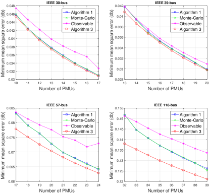
Figure 1: MMSE by different methods

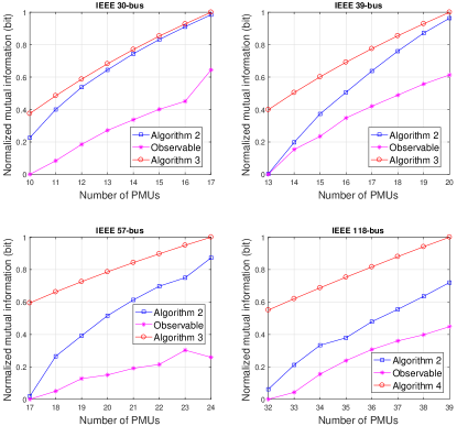
Figure 2: MI by different methods

Table II provides numerical details of Algorithm 1, Algorithm 2 and Algorithm 3. The value of the penalized parameter $\mu$ in implementing Algorithm 1 and Algorithm 2 is given by the second and fourth column, while the average CPU time is given by the third and fifth column. The last two columns provide average CPU time by Algorithm 3 in solving MMSE and MI. Algorithm 3 needs much less time for small-scale networks but its computational cost increases dramatically with the growth of network size. On the other hand, the CPU time of Algorithm 1 and Algorithm 2 increases moderately when the size of networks grows, demonstrating their scalability and superiority in addressing large-scale networks.

TABLE II: Numerical details of Algorithm 1, Algorithm 2 and Algorithm 3

IEEE	Alg. 1		Alg. 2		CPU (s) of Alg. 3
	$\mu$	Avg. T. (s)	$\mu$	CPU (s)	MMSE	MI
30-bus	0.1	65.78	1	62.94	4.01	3.17
39-bus	0.1	79.73	1	77.25	11.58	7.98
57-bus	1	80.47	10	81.14	49.09	46.03
118-bus	1	216.31	10	193.24	1222.11	2142.08

For problem (19), Kekatos et al [14] relaxed the integer constraint $\boldsymbol{x}\in\{0,1\}^{N}$ to the box constraint $\boldsymbol{x}\in[0,1]^{N}$ to formulate a convex problem and then round the $S$ largest values of the solution of this convex program to $1$. Obviously, their solution is hardly optimal in any sense. Fig. 3 compares the MMSE values of problem (19) founded by Algorithm 3 and by Kekatos et al [14]. The former clearly outperforms the latter, especially for large scale networks.

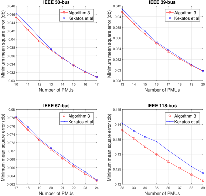
Figure 3: MMSE found by Algorithm 3 and by [14]

Due to space limitation, only IEEE 30-bus and IEEE-39 networks are selected for MMSE results solved by Algorithm 1 under the constraint (10) of depth-of-one unobservability. Fig. 4 provides MMSE performance obtained via Algorithm 1 (under the constraint (10)) and Algorithm 3 (without any observability constraints), while Fig. 5 provides the number of bus left unobservable (for IEEE 30-bus). As expected, Algorithm 3 achieves a better MMSE but leaves more buses unobservable because it sacrifices buses to achieve the averaged performance.

For IEEE 57-bus network and IEEE 118-bus network, Fig.6 presents the number of iterations needed for the convergence of Algorithm 3 for MMSE and MI, respectively.

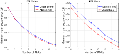
Figure 4: MMSE found by Algorithm 1 under depth-of-one unobservability condition and Algorithm 3 without any observability constraints

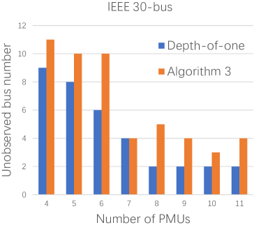
Figure 5: Number of buses left unobserved by Algorithm 1 under depth-of-one unobservability condition and Algorithm 3 without any observability constraints for IEEE 30-bus network

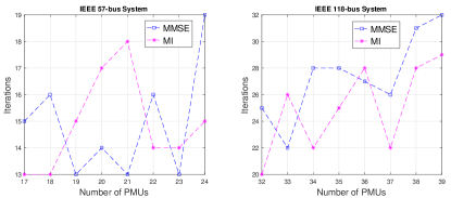
Figure 6: Number of iterations required for the convergence of Algorithm 3

Given different tolerances $\epsilon$, the required minimum number of PMUs can be obtained by Algorithm 4. For the case of $f=F_{e}$, the results are presented in Fig.7.

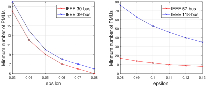
Figure 7: Minimum number of PMUs required versus different values of tolerance level $\epsilon$ for MMSE

VI Conclusions

In this paper, we have considered PMU placement optimization to minimize the mean squared error or maximize the mutual information between the measurement outputs and phasor states under a fixed number of PMUs and different observability conditions. These binary optimization problems are very computationally challenging due to high nonlinearity of the objective functions. Nevertheless, we have developed the scalable algorithms for their computational solution, which result at least in local optimal solutions. We also developed extremely efficient algorithms of very low computational complexity for cases of absent observability. The viability of our proposed algorithms has been confirmed through simulations with benchmark IEEE grids. The algorithmic developments for PMU placement optimization involving other practical constraints such as branch outages are under way.

Appendix: Fundamental Inequalities

Let $\mathbb{R}^{N}_{+}:=\{x\in\mathbb{R}^{N}:x_{k}\geq 0,k\in{\cal N}\}$ and ${\sf int}(\mathbb{R}^{N}_{+}):=\{x\in\mathbb{R}^{N}:x_{k}>0,k\in{\cal N}\}$. For $A_{0}\succ 0$ and $A_{k}\succeq 0$, $k\in{\cal N}$ let $\Phi(\boldsymbol{x}):=(A_{0}+\displaystyle\sum_{k\in{\cal N}}\frac{1}{x_{k}}A_{k})^{-1},$ and $\Psi(\boldsymbol{x}):=(A_{0}+\displaystyle\sum_{k=1}^{N}x_{k}A_{k})^{-1}$. Recall the following result [33, Th.1]:

Theorem 1

Function $\varphi(\boldsymbol{x})={\rm Trace}(\Phi(\boldsymbol{x}))$ is concave in the domain ${\sf int}(\mathbb{R}^{N}_{+})$, so for all $\boldsymbol{x}\in{\sf int}(\mathbb{R}^{N}_{+})$ and $\bar{\boldsymbol{x}}\in{\sf int}(\mathbb{R}^{N}_{+})$ one has

$$\begin{array}[]{lll}\varphi(\boldsymbol{x})&\leq&\varphi(\bar{\boldsymbol{x}})+\langle\nabla\varphi(\bar{\boldsymbol{x}}),\boldsymbol{x}-\bar{\boldsymbol{x}}\rangle\\ &=&{\rm Trace}\left(\Phi^{2}(\bar{\boldsymbol{x}})A_{0}\right)+\displaystyle\sum_{k\in{\cal N}}\frac{x_{k}}{\bar{x}_{k}^{2}}{\rm Trace}\left(\Phi^{2}(\bar{\boldsymbol{x}})A_{k}\right).\end{array}$$

Therefore,

$${\rm Trace}(\Psi(\boldsymbol{x})) \leq {\rm Trace}\left((\Psi(\bar{\boldsymbol{x}}))^{2}A_{0}\right)$$ (23)

$$+\displaystyle\sum_{k\in{\cal N}}\frac{\bar{x}_{k}^{2}}{x_{k}}{\rm Trace}\left((\Psi(\bar{\boldsymbol{x}}))^{2}A_{k}\right).$$

Next,

Theorem 2

For $A\succ 0$ function $\ln|A+H\mathbf{X}^{-1}H^{H}|$ is convex in $\mathbf{X}\succ 0$.

Proof. Since $(A+H\mathbf{X}^{-1}H^{H})^{-1}=A^{-1}-A^{-1}(H^{H}A^{-1}H+\mathbf{X})^{-1}A^{-1}$, by [34, Appendix B], function

$$f(\mathbf{X}):=A^{-1}-A^{-1}(H^{H}A^{-1}H+\mathbf{X})^{-1}A^{-1}$$

is concave, i.e. $f(\alpha\mathbf{X}+\beta\mathbf{Y})\succ\alpha f(\mathbf{X})+\beta f(\mathbf{Y})\quad\ \forall\ \mathbf{X}\succ 0,\mathbf{Y}\succ 0$, and $\alpha\geq 0,\beta\geq 0,\alpha+\beta=1$. Therefore $\ln|f(\alpha\mathbf{X}+\beta\mathbf{Y})|\geq\ln|\alpha f(\mathbf{X})+\beta f(\mathbf{Y})|\geq\alpha\ln|f(\mathbf{X})|+\beta\ln|f(\mathbf{Y})|$, showing that $\ln|A+H\mathbf{X}^{-1}H^{H}|^{-1}=-\ln|A+H\mathbf{X}^{-1}H^{H}|$ is concave in $\mathbf{X}$.∎

The following Theorem is a direct consequence of Theorem 2.

Theorem 3

Function $\phi(\boldsymbol{x})=-\ln|\Phi(\boldsymbol{x})|$ is convex in the domain ${\sf int}(\mathbb{R}^{N}_{+})$, so for all $\boldsymbol{x}\in{\sf int}(\mathbb{R}^{N}_{+})$ and $\bar{\boldsymbol{x}}\in{\sf int}(\mathbb{R}^{N}_{+})$ one has

$$\begin{array}[]{lll}\phi(\boldsymbol{x})&\geq&\phi(\bar{\boldsymbol{x}})+\langle\nabla\phi(\bar{\boldsymbol{x}}),\boldsymbol{x}-\bar{\boldsymbol{x}}\rangle\\ &=&-\ln|\Phi(\bar{\boldsymbol{x}})|+\displaystyle{\rm Trace}\left((\Phi(\bar{\boldsymbol{x}}))^{-1}(\sum_{k\in{\cal N}}\frac{1}{\bar{x}_{k}}A_{k})\right)\\ &&\displaystyle-\sum_{k\in{\cal N}}\frac{x_{k}}{\bar{x}_{k}^{2}}{\rm Trace}\left((\Phi(\bar{\boldsymbol{x}}))^{-1}A_{k}\right).\end{array}$$

Therefore,

$$-\ln|\Psi(\boldsymbol{x})|\geq-\ln|\Psi(\bar{\boldsymbol{x}})|+{\rm Trace}\left(\Psi(\bar{\boldsymbol{x}})(\sum_{k\in{\cal N}}\bar{x}_{k}A_{k})\right)$$

$$-\displaystyle\sum_{k\in{\cal N}}\frac{\bar{x}_{k}^{2}}{x_{k}}{\rm Trace}\left(\Psi(\bar{\boldsymbol{x}})A_{k}\right).$$ (24)

References

• [1] J. De La Ree, V. Centeno, J. S. Thorp, and A. G. Phadke, “Synchronized phasor measurement applications in power systems,” IEEE Trans. smart grid, vol. 1, no. 1, pp. 20–27, 2010.
• [2] A. G. Phadke and J. S. Thorp, Synchronized Phasor Measurements and Their Applications. New York: Springer, 2008.
• [3] J. A. Momoh, R. Adapa, and M. El-Hawary, “A review of selected optimal power flow literature to 1993. i. nonlinear and quadratic programming approaches,” IEEE Trans. Power Systems, vol. 14, no. 1, pp. 96–104, 1999.
• [4] J. Zhao, G. Zhang, K. Das, G. N. Korres, N. M. Manousakis, A. K. Sinha, and Z. He, “Power system real-time monitoring by using PMU-based robust state estimation method,” IEEE Trans. Smart Grid, vol. 7, no. 1, pp. 300–309, 2016.
• [5] C.-W. Ten, A. Ginter, and R. Bulbul, “Cyber-based contingency analysis,” IEEE Trans. Power Systems, vol. 31, no. 4, pp. 3040–3050, 2016.
• [6] B. Gou, “Optimal placement of PMUs by integer linear programming,” IEEE Trans. Power Systems, vol. 23, no. 3, pp. 1525–1526, 2008.
• [7] B. Gou, “Generalized integer linear programming formulation for optimal PMU placement,” IEEE Trans. Power Systems, vol. 23, no. 3, pp. 1099–1104, 2008.
• [8] R. F. Nuqui and A. G. Phadke, “Phasor measurement unit placement techniques for complete and incomplete observability,” IEEE Trans. Power Delivery, vol. 20, no. 4, pp. 2381–2388, 2005.
• [9] S. Chakrabarti and E. Kyriakides, “Optimal placement of phasor measurement units for power system observability,” IEEE Trans. Power Systems, vol. 23, no. 3, pp. 1433–1440, 2008.
• [10] M. Hajian, A. M. Ranjbar, T. Amraee, and B. Mozafari, “Optimal placement of PMUs to maintain network observability using a modified bpso algorithm,” Int. J. Elect. Power Energy Syst., vol. 33, no. 1, pp. 28–34, 2011.
• [11] S. Chakrabarti, E. Kyriakides, and D. G. Eliades, “Placement of synchronized measurements for power system observability,” IEEE Trans. Power Delivery, vol. 24, no. 1, pp. 12–19, 2009.
• [12] K. G. Khajeh, E. Bashar, A. M. Rad, and G. B. Gharehpetian, “Integrated model considering effects of zero injection buses and conventional measurements on optimal PMU placement,” IEEE Trans. Smart Grid, vol. 8, no. 2, pp. 1006–1013, 2017.
• [13] M. J. Rice and G. T. Heydt, “Power systems state estimation accuracy enhancement through the use of PMU measurements,” in IEEE PES Transmission and Distribution Conf. and Exposition, 2006.
• [14] V. Kekatos, G. B. Giannakis, and B. Wollenberg, “Optimal placement of phasor measurement units via convex relaxation,” IEEE Trans. Power Systems, vol. 27, no. 3, pp. 1521–1530, 2012.
• [15] Q. Li, T. Cui, Y. Weng, R. Negi, F. Franchetti, and M. D. Ilic, “An information-theoretic approach to PMU placement in electric power systems,” IEEE Trans. Smart Grid, vol. 4, no. 1, pp. 446–456, 2013.
• [16] G. Krumpholz, K. Clements, and P. Davis, “Power system observability: a practical algorithm using network topology,” IEEE Trans. Power Apparatus and Systems, no. 4, pp. 1534–1542, 1980.
• [17] A. Schellenberg, W. Rosehart, and J. Aguado, “Cumulant-based probabilistic optimal power flow (P-OPF) with gaussian and gamma distributions,” IEEE Trans. Power Systems, vol. 20, no. 2, pp. 773–781, 2005.
• [18] J. Grainger and J. W. Stevenson, Power System Analysis. New York: McGraw-Hill, 1994.
• [19] J. De La Ree, V. C. anf J. Thorp, and A. Phadke, “Synchronized phasor measurement applications in power systems,” IEEE Trans. Smart Grid, vol. 1, pp. 20–27, Jun. 2010.
• [20] H. V. Poor, An Introduction to Signal Detection and Estimation (second edition). New York: Springer-Verlag, 1994.
• [21] H. D. Tuan, D. H. Pham, B. Vo, and T. Q. Nguyen, “Entropy of general Gaussian distributions and MIMO channel capacity maximizing precoder and decoder,” in Proc. 2007 IEEE Inter. Conf. Acous. Speech Signal Process (ICASSP 07), pp. III–325–III–328, May 2007.
• [22] R. Kavasseri and S. K. Srinivasan, “Joint placement of phasor and power flow measurements for observability of power systems,” IEEE Trans. Power Systems, vol. 26, no. 4, pp. 1929–1936, 2011.
• [23] M. Göl and A. Abur, “Observability and criticality analyses for power systems measured by phasor measurements,” IEEE Trans. Power Systems, vol. 28, no. 3, pp. 3319–3326, 2013.
• [24] H. Tuy, Convex Analysis and Global Optimization (second edition). Springer, 2016.
• [25] E. Che, H. D. Tuan, and H. H. Nguyen, “Joint optimization of cooperative beamforming and relay assignment in multi-user wireless relay networks,” IEEE Trans. Wirel. Commun., vol. 13, pp. 5481–5495, Oct. 2014.
• [26] H. H. M. Tam, H. D. Tuan, D. T. Ngo, T. Q. Duong, and H. V. Poor, “Joint load balancing and interference management for small-cell heterogeneous networks with limited backhaul capacity,” IEEE Trans. Wirel. Commun., vol. 16, pp. 872–884, Feb. 2017.
• [27] J. Chen and A. Abur, “Placement of PMUs to enable bad data detection in state estimation,” IEEE Trans. Power Systems, vol. 21, pp. 1608–1615, Nov 2006.
• [28] H. D. Tuan, T. T. Son, H. Tuy, and H. H. Nguyen, “Optimum multi-user detection by nonsmooth optimization,” in 2011 IEEE International Conference on Acoustics, Speech and Signal Processing (ICASSP), pp. 3444–3447, 2011.
• [29] B. A. Cipra, “The best of the 20th century: editors name top 10 algorithms,” SIAM News, vol. 33, pp. 1–2, Dec. 2000.
• [30] R. D. Zimmerman, C. E. Murillo-Sánchez, and R. J. Thomas, “Matpower: Steady-state operations, planning, and analysis tools for power systems research and education,” IEEE Trans. Power Systems,, vol. 26, pp. 12–19, Feb 2011.
• [31] J. Sturm, “Using SeDuMi 1.02, a MATLAB toolbox for optimization over symmetric cones,” Optimization Methods and Software, vol. 11–12, pp. 625–653, 1999.
• [32] “CPLEX optimizer.” https://www.ibm.com/analytics/data-science/prescriptive-analytics/cplex-optimizer. Accessed: 2018-02-14.
• [33] J. A. Bengua, H. D. Tuan, T. Q. Duong, and H. V. Poor, “Joint sensor and relay power control in tracking Gaussian mixture targets by wireless sensor networks,” IEEE Trans. Signal Process., vol. 66, no. 2, pp. 492–506, 2018.
• [34] U. Rashid, H. D. Tuan, H. H. Kha, and H. H. Nguyen, “Joint optimization of source precoding and relay beamforming in wireless MIMO relay networks,” IEEE Trans. Commun., vol. 62, pp. 488–499, Feb. 2014.