Conditional probability calculation using restricted Boltzmann machine with application to system identification

Abstract

There are many advantages to use probability method for nonlinear system identification, such as the noises and outliers in the data set do not affect the probability models significantly; the input features can be extracted in probability forms. The biggest obstacle of the probability model is the probability distributions are not easy to be obtained.

In this paper, we form the nonlinear system identification into solving the conditional probability. Then we modify the restricted Boltzmann machine (RBM), such that the joint probability, input distribution, and the conditional probability can be calculated by the RBM training. Binary encoding and continue valued methods are discussed. The universal approximation analysis for the conditional probability based modelling is proposed. We use two benchmark nonlinear systems to compare our probability modelling method with the other black-box modeling methods. The results show that this novel method is much better when there are big noises and the system dynamics are complex.

Keywords: system identification, conditional probability, restricted Boltzmann machine

1 Introduction

Data based system identification is to use the experimental data from system input and output. Usually, the mathematical model of its input-output behavior is applied to predict the system response (output) from the excitation (input) to the system. There is always uncertainty when a model is chosen to represent the system. Including probability theory in dynamic system identification can improve the modeling capability with respect to noise and uncertainties [1]. The common probability approaches for system identification parameterize the model and apply Bayes’ Theorem [2], such as maximizing the posterior [3], maximizing the likelihood function [5], or matching the output by least-squares method [4]. There are several computational difficulties with the above estimation methods, for example, the probability models for the likelihood construction cannot be expected to be perfect; the parameter estimations are often not unique, because the true values of the parameters may not exist.

In the sense of probability theory, the objective of system modeling is to find the best conditional probability distribution $P(y|\mathbf{x})$ [6], where $\mathbf{x}$ is the input and $y$ is the output. So the system identification can be transformed to the calculation of the conditional probability distribution, it is no longer the parameter estimation problem. For nonlinear system identification, there are two correlated time series, the input $\mathbf{x}$ and the output $y$. The popular Monte Carlo method cannot obtain the best prediction of $y$ from the conditional probability between of $\mathbf{x}$ and $y$ [7].

Recent results, show that restricted Boltzmann machine (RBM) [8] can learn the probability distribution of the input data using the unsupervised learning method, and obtains their hidden features [9][10]. These latent features help the RBM to obtain better representations of the empirical distribution. Feature extractions and pre-training are two important properties of the RBMs for solving classification problems in the past years [11].

RBMs are also applied for data regression and time series modeling. With RBM pre-training, the prediction accuracy of the time series can be improved [12][13]. The hidden and visible units of normal RBM are binary. The prediction accuracy of the time series with continuous values are not satisfied [14]. In [15], the binary units are replaced by linear units with Gaussian noise. The denoising autoencoders are used for continuous valued data in [16]. In [17], the time series are assumed to have the Gaussian property.

In order to find the relation between the input $\mathbf{x}$ and the output $y$, the RBM is used to obtain the conditional probabilities between $\mathbf{x}$ and the hidden units of the RBM in our previous papers [18][19]. The hidden units are used as the initial weights of neural networks, then the supervised learning is implemented to obtain the inpu-output relation, $y=f\left(\mathbf{x}\right)$. To the best of our knowledge, conditional probability approach for system identification has not been still applied in the literature.

In this paper, we use the conditional probability to model the nonlinear system by RBM training. The RBMs are modified, such that the input distribution, the joint probability $P(y,x),$ and the conditional probability $P(y|x)$ can be calculated. We proposed two probability calculation methods: binary encoding and continuous values. Probability gradient algorithm is used to maximize the log-likelihood of the conditional probability between the input and output. The comparisons with the other black-box identification methods are carried out using two nonlinear benchmark systems.

2 Nonlinear system modeling with conditional probability

We use the following difference equation to describe a discrete-time nonlinear system,

$$y(k)=f\left[\mathbf{x}\left(k\right),\xi\left(k\right),\cdots\xi\left(k-n_{\xi}\right)\right]$$ (1)

where $\xi\left(k\right)$ are noise sequences, $f\left(\cdot\right)$ is an unknown nonlinear function,

$$\mathbf{x}\left(k\right)=[y\left(k-1\right),\cdots y\left(k-n_{y}\right),u\left(k\right),\cdots u\left(k-n_{u}\right)]^{T}$$ (2)

representing the plant dynamics, $u\left(k\right)$ and $y\left(k\right)$ are the measurable input and output of the nonlinear plant, $n_{y}$ and $n_{u}$ correspond to the system order, $n_{\xi}$ is the maximum lag for the noise. $\mathbf{x}\left(k\right)\in\Re^{n}$ can be regarded as a new input to the nonlinear function $f\left(\cdot\right).$ It is the well known NARMAX model [20].

The objective of the system modeling is to use the input-output data, to construct a model $\hat{y}(k)=\hat{f}\left[\mathbf{x}\left(k\right)\right],$ such that $\hat{y}(k)\rightarrow y(k).$ If the lost function is defined by

$$L=\sum_{k}\left[y(k)-\hat{f}\left[\mathbf{x}\left(k\right)\right]\right]^{2}$$

The mathematical expectation of the modeling error is

$$E\left\{\left[y(k)-\hat{f}\left[\mathbf{x}\left(k\right)\right]\right]^{2}\right\}=\int\left[y-\hat{f}\left(x\right)\right]^{2}p\left(dx,dy\right)$$ (3)

where the joint probability satisfies

$$p\left(X,Y\right)=p\left(X\right)p\left(Y\mid X\right)$$

Here $p\left(Y\mid X\right)$ is the conditional probability. The modeling error (3) becomes

$$\begin{array}[c]{c}E\left\{\left[y(k)-\hat{f}\left[\mathbf{x}\left(k\right)\right]\right]^{2}\right\}=\int\left[y-\hat{f}\right]^{2}p\left(dx\right)p\left(dy\mid dx\right)\\ =E_{\mathbf{x}}E_{\left(y\mid\mathbf{x}\right)}\left\{\left[y-\hat{f}\right]^{2}\mid\mathbf{x}\right\}\end{array}$$

The system identification becomes the minimization problem as

$$\min E\left\{\left[y-\hat{f}\right]^{2}\right\}\rightarrow\min_{\hat{f}}E_{\left(y\mid\mathbf{x}\right)}\left\{\left[y-\hat{f}\right]^{2}\mid\mathbf{x}\right\}$$

The best prediction of $y$ at $\mathbf{x}=x$ is the conditional mean (conditional expectation) as

$$\hat{f}\left[\mathbf{x}\left(k\right)\right]=E\left\{\hat{y}\mid\mathbf{x}\right\}$$

The nonlinear system modeling becomes

$$\max_{\theta}\left\{p\left(y\mid\mathbf{x},\Lambda\right)\right\}$$ (4)

where $\Lambda$ is the parameter vector of the model $\hat{f}.$ The existing methods use some probability approaches, such as Bayes’ Theorem, to estimate $\Lambda$. In this paper, we do not use parameterized models. We will calculate the conditional probability distribution $p\left[y\left(k\right)|\mathbf{x}\left(k\right)\right]$ directly.

The loss function for the conditional distribution $p(y|\mathbf{x})$ is defined as

$$J_{o}(D)=\sum_{D}\log p\left(y|\mathbf{x}\right)$$ (5)

where $D=\{\mathbf{x}(k),y(k)\},$ is the training set, $\mathbf{x}(k)$ and $y(k)$ are the $k$-th training input vector and output respectively. So the object of the nonlinear system identification (4) becomes

$$\max_{\Lambda}\left[\sum_{D}\log p\left(y|\mathbf{x}\right)\right]$$ (6)

In this paper, we use the restricted Boltzmann machine (RBM) to obtain the best conditional probability. RBM is a stochastic neural network. It can learn the probability distribution of given data set. The input (or the visible nodes) to the RBM is $\mathbf{x}\left(k\right)=\left[x_{1}\cdots x_{n}\right]\in R^{n}$. The output (or the hidden nodes) of the RBM is $h=\left[\bar{h}_{1}\cdots\bar{h}_{s}\right]\in R^{s}$. For the $i-th$ hidden node and the $j-th$ visible node, the conditional probabilities are calculated as

$$\begin{array}[c]{l}p\left(\bar{h}_{i}=1\mid\mathbf{x}\right)=\phi\left[W\mathbf{x}+b\right]\\ p\left(x_{j}=1\mid h\right)=\phi\left[W^{T}h+c\right]\end{array}$$ (7)

where $\bar{h}_{i}=\left\{\begin{array}[c]{cc}1&a<p\left(\bar{h}_{i}=1\mid\mathbf{x}\right)\\ 0&a\geq p\left(\bar{h}_{i}=1\mid\mathbf{x}\right)\end{array}\right.$, $\phi$ is the Sigmoid function, $W$ is the weight matrix, $a$ is a number sampled from the uniform distribution over $[0,1]$, $b$ and $c$ are visible and hidden biases respectively, $i=1,\ldots,s$, $j=1,\ldots,n.$ The probability vector $h$ is defined as

$$h=\left[p\left(\bar{h}_{1}=1\mid\mathbf{x}\right)\cdots p\left(\bar{h}_{s}=1\mid\mathbf{x}\right)\right]=\left[h_{1}\cdots h_{s}\right]$$

The training object of the RBM is to modify the parameters $\left[W,b,c\right],$ such that the probability distribution of the hidden units $p$ is near to the distribution of the input $q$. We use Kullback-Liebler (KL) divergence to measure the distance between two probability distributions $p$ and

$$KL\left(p,q\right)=\sum_{D}q\left(\mathbf{x}\right)\log\frac{q\left(\mathbf{x}\right)}{p\left(\mathbf{x}\right)}=\sum_{D}q\left(x\right)\log q\left(x\right)-\sum_{D}q\left(x\right)\log p\left(x\right)$$ (8)

Here the first term $\sum_{x}q\left(x\right)\log q\left(x\right)$ is the entropy of the input. It is independent of the RBM training.

The RBM training object becomes

$$\min KL\left(p,q\right)\rightarrow\max\sum_{D}q\left(x\right)\log p\left(x\right)$$ (9)

$q\left(x\right)$ cannot be obtained directly, it is estimated by Monte Carlo method

$$\sum_{D}q\left(x\right)\log p\left(x\right)\approx\frac{1}{n}\sum_{D}\log p\left(x\right)$$

where $n$ is the number of training data. So

$$\min KL\left(p,q\right)\rightarrow\max\sum_{x}\log p\left(x\right)$$

The following lemma and theorem give the universal approximation of the nonlinear system (1) with the conditional probability $p(y|\mathbf{x})$ and the RBM.

Lemma 1

Any marginal probability distribution $p(\mathbf{x}),$ $\mathbf{x}\in\{0,1\}^{r}$, can be approximated arbitrarily well in the sense of the KL divergence (8) by then RBM with $r+1$ hidden units, where $r$ is the number of input vector whose probability is not $0$ [22].

Theorem 1

If the hidden units of the RBM (7) is big enough, the conditional probability $p(y|\mathbf{x})$ of the nonlinear system (1) can be approximated arbitrarily well by an RBM and the pair $(\mathbf{x},y),$ in the sense of the KL divergence (8).

Proof. Consider the nonlinear system (1), the vectors $\mathbf{x}$ and $y$ are from the finite sets $\left\{\mathbf{x}_{1},...,\mathbf{x}_{k,}...,\mathbf{x}_{r_{0}}\right\}$ and $\left\{y_{1},...,y_{l,}...,y_{m_{0}}\right\}$. For each pair $\left(\mathbf{x}_{k},y_{l}\right)$, the conditional probability distribution is $p(y_{l}|\mathbf{x}_{k}),$ $k=1,...,r_{0}$ and $l=1,...m_{0}$. The conditional probability of the pair is

$$p(y_{l}|\mathbf{x}_{k})=\frac{p(\mathbf{x}_{k},y_{l})}{p(\mathbf{x}_{k})}=\frac{p(\mathbf{x}_{k},y_{l})}{\sum_{j}p(\mathbf{x}_{k},y_{j})}$$ (10)

Here the value of $p(y_{l}|\mathbf{x}_{k})$ is assumed to be known. The term $\sum_{j}p(\mathbf{x}_{k},y_{j})$ can be separated as $\sum_{j\neq l}p(\mathbf{x}_{k},y_{j})$ and $p(\mathbf{x}_{k},y_{l}).$ From (10),

$$p(\mathbf{x}_{k},y_{l})=\frac{p(y_{l}|\mathbf{x}_{k})\sum_{j\neq l}p(\mathbf{x}_{k},y_{j})}{1-p(y_{l}|\mathbf{x}_{k})}$$ (11)

For each pair $\left(\mathbf{x}_{k},y_{l}\right)$, $p(\mathbf{x}_{k},y_{l})$ can be calculated for the indexes $k$ and $l$ from (11). There are $r_{0}\times m_{0}$ equations. They are considered as the desired conditional distribution of $p(y|\mathbf{x})$, i.e., we can use $p(\mathbf{x}_{k},y_{l})$ to create the distribution which contains the original conditional distribution $p(y|\mathbf{x})$. Now we apply all pairs $\left(\mathbf{x}_{k},y_{l}\right),$ $k=1,...,r_{0}$ and $l=1,...m_{0},$ to the RBM whose hidden unit number is $r_{0}\times m_{0}+1.$

If $\mathbf{x}_{k}$ and $y_{l}$ are binary values, $\mathbf{x}\in\{0,1\}^{m},$ $y\in\{0,1\}^{r},$ we define the pair $(\mathbf{x}_{k},y_{l})$ as a single random variable $z_{kl},$ $p(z_{kl})=p(\mathbf{x}_{k},y_{l}).$ From Lemma 1, we can construct an RBM with the most $r_{0}\times m_{0}+1$ hidden units (all input nodes have non-zero probability), which models the distribution $p(z_{kl})$, with the desired conditional distribution of $p(y|\mathbf{x}).$

If $\mathbf{x}_{k}$ and $y_{l}$ are not binary values, we encode the input variable $\mathbf{x}$ and $y$ into binary values $\left\{0,1\right\}$ with the resolution of $m$ bits. This means that $y\left(k\right)$ is encoded into $2^{m}$ different levels with the step of $1/(2^{m}-1).$ Similarly, the control $\mathbf{x}\left(k\right)$ is encoded into $2^{m}$ different levels,

$$\begin{array}[c]{l}\mathbf{x}\in\Re^{n}\longrightarrow\mathbf{x}\in\{0,1\}^{n\times m}\\ y\in\Re\longrightarrow y\in\{0,1\}^{m}\end{array}$$ (12)

We can construct an RBM with at most $\left(n\times m\times r_{0}\right)\times\left(m\times m_{0}\right)+1$ hidden units. The desired conditional distribution of $p(y|\mathbf{x})$ can be approximated arbitrarily well in the sense of the KL divergence.   

The above theorem can be regarded as the probability version of the universal approximation theory of neural networks [23][24]. One RBM with one hidden layer can learn the probability $p(y|\mathbf{x})$ of the nonlinear system in any accuracy, the hidden node number of the RBM should be the same as total data number. This cause serious over-fitting and computational problems.

In order to improve the approximation accuracy, we can use several RBMs with cascade connection. It is called deep Boltzmann machines (or deep belief nets) [21]. Instead of using more hidden nodes, it use more layers (or more RBMs) to learn the probability $p(y|\mathbf{x})$ to avoid the above problems. This architecture is shown in Figure 1. Each RBM has the form of (7). The output of the current RBM is its hidden vector $h$. It is the input of the next RBM.

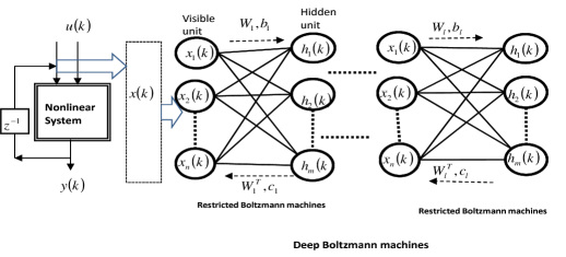
Figure 1: Deep Boltzmann machines for conditional probability of nonlinear system

3 Joint distribution for nonlinear system identification

Because the conditional probability

$$p(y|\mathbf{x})=\frac{p(\mathbf{x,}y)}{p(\mathbf{x})},\quad\log p(y\mathbf{|x})=\log p(\mathbf{x,}y)-\log p(\mathbf{x})$$ (13)

The object of system identification (6) can also be formed as

$$\max_{\Lambda}\left[\sum_{D}\log p(\mathbf{x,}y)\right]\text{ and }\min_{\Lambda}\left[-\sum_{D}\log p(\mathbf{x})\right]$$ (14)

The identification object (14) is an alternative method of the conditional probability (6), which needs the joint distribution $\sum_{D}\log p(\mathbf{x,}y)$ and the input distribution $\sum_{D}\log p(\mathbf{x})$. It is more easy to calculate the joint distribution than the conditional probability. However, it is impossible to optimize $\sum_{D}\log p(\mathbf{x,}y)$ and $\sum_{D}\log p(\mathbf{x})$ with $D=\{\mathbf{x}(k),y(k)\}$ at same time. We can use part of the training data $\mathbf{x}$ to minimize $\sum_{D}\log p(\mathbf{x})$ first, then use the rest of data to maximize the joint probability $\sum_{D}\log p(\mathbf{x,}y)$.

In our previous works [18][19], we first use the input data $\mathbf{x}$ to pre-train the RBM. The training results are used as the initial weights of neural networks. Then we used the supervised learning to train the neural model. In this paper, after the unsupervised learning for $\sum_{D}\log p(\mathbf{x}),$ we train the RBM to obtain $\max_{\Lambda}\left[\sum_{D}\log p(\mathbf{x,}y)\right].$ For the nonlinear system identification, its a sub-optimization process.

3.1 Pre-training for $p(\mathbf{x})$

The goal of the unsupervised training is to obtain $\min_{\Lambda}\left[\sum_{D}\log p(\mathbf{x})\right]$ by reconstructing the RBM. The parameters $\Lambda=\left[W,b,c\right]$ are trained such that $h$ is the representation of $\mathbf{x}$ (feature extraction). The probability distribution $p\left(\mathbf{x}\right)$ is the following energy-based model

$$p(\mathbf{x})=\sum_{h}p(\mathbf{x},h)=\sum_{h}\frac{e^{-E(\mathbf{x},h)}}{Z}$$ (15)

where $Z=\sum_{h}\sum_{\mathbf{x}}e^{-E(\mathbf{x},h)}$ denotes the sums over all possible values of $h$ and $\mathbf{x,}$ $E(x,h)$ is the energy function which is defined by

$$E\left(\mathbf{x},h\right)=-c^{T}\mathbf{x}-b^{T}h-h^{T}W\mathbf{x}$$ (16)

The loss function for the training is

$$L\left(\Lambda\right)=\log{\displaystyle\prod\limits_{\mathbf{x}}}p\left(\mathbf{x}\right)=\log\left[\sum_{\mathbf{x}}e^{-E\left(\mathbf{x},h\right)}\right]-\log\left[\sum_{\mathbf{x},h}e^{-E\left(\mathbf{x},h\right)}\right]$$

The weights are updated as

$$\Lambda\left(k+1\right)=\Lambda\left(k\right)-\eta_{1}\frac{\partial\left[-\log p\left(\mathbf{x}\right)\right]}{\partial\Lambda}$$ (17)

where $\eta_{1}$ is the learning rate, $\frac{\partial\log p\left(\mathbf{x}\right)}{\partial\Lambda}=\sum_{x}p\left(\mathbf{x}\right)\frac{\partial\digamma(\mathbf{x})}{\partial\Lambda}-\frac{\partial\digamma(\mathbf{x})}{\partial\Lambda},$ $\digamma(\mathbf{x})$ is the free energy defined as

$$\digamma(\mathbf{x})=\sum_{\mathbf{x}}\log p\left(\mathbf{x}\right)=-c^{T}\mathbf{x}-\sum_{p=1}^{l_{i}}\log\sum_{h_{p}}e^{h_{p}\left(b_{p}+W_{p}\mathbf{x}\right)}$$

Here $\sum_{z}p\left(\mathbf{x}\right)\frac{\partial\digamma(\mathbf{x})}{\partial\Lambda}$ is estimated by the Monte Carlo sampling,

$$\sum_{z}p\left(\mathbf{x}\right)\frac{\partial\digamma(\mathbf{x})}{\partial\Lambda}\thickapprox\frac{1}{s}\sum_{z\in S}\frac{\partial\digamma(\mathbf{x})}{\partial\Lambda}$$ (18)

The above algorithm is for one RBM. The training process of multiple RBMs is shown in Figure 2. After the first model is trained, their weights are fixed. The codes or hidden representations of the first model are sent to the second model. The second model is trained using input $h_{1}\left(k\right)\in\Re^{l_{1}}$ and it generates its hidden representations $h_{2}\left(k\right)\in\Re^{l_{2}},$ which is the input of the third model.

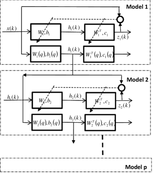
Figure 2: Cascade traning of multipe RBMs

If $\mathbf{x}$ is encoded into binary values as (12), i.e., $x_{t}\in\left\{0,1\right\},$ the binary hidden units are $h_{p}\in\left\{0,1\right\},$

$$\begin{array}[c]{l}p\left(h_{p}=1|\mathbf{x}\right)_{p=1\cdots l_{i}}=\phi\left[W_{p}\mathbf{x}+b_{p}\right]\\ p\left(x_{t}=1|h\right)_{t=1\cdots l_{i-1}}=\phi\left[W_{t}^{T}h+c_{t}\right]\end{array}$$ (19)

If the input $\mathbf{x}$ uses continuous value. We first normalize $\mathbf{x}$ in $[0,1].$ The conditional probability for the $j$-th visible node is

$$P(x_{j}|h)=\frac{e^{(V_{j}^{T}\overline{h}+c_{j})x_{j}}}{\int_{\widehat{x}_{j}}e^{(V_{j}^{T}\overline{h}+c_{j})\widehat{x}_{j}}d\widehat{x}_{j}}$$

Since $x_{j}\in[0,1],$ the probability distribution is $P(x_{j}|h)=\frac{a_{j}e^{a_{j}x_{j}}}{e^{a_{j}}-1},$ $a_{j}=V_{j}^{T}\overline{h}+c_{j}$. The accumulative conditional probability from sampling process is

$$P_{C}(x_{j}|h)=\frac{e^{a_{j}x_{j}}-1}{e^{a_{j}}-1}$$ (20)

The expected value of the distribution is $E[x_{j}]=\frac{1}{1-e^{-a_{j}}}-\frac{1}{a_{j}}$.

3.2 Joint distribution $p(\mathbf{x},y)$

Here we will discuss how to maximize the joint probability $J_{c}(D)=\sum_{D}\log p(\mathbf{x,}y)$ by RBM training. The parameters of RBMs are updated as

$$\Lambda\left(k+1\right)=\Lambda\left(k\right)-\eta_{2}\frac{\partial\left[\log p(\mathbf{x,}y)\right]}{\partial\Lambda}$$ (21)

where $\eta_{2}$ is the learning rate. By the chain rule $p(\mathbf{x},y,h)=p(h|\mathbf{x},y)p(\mathbf{x,}y)$,

$$\frac{\partial\log p(\mathbf{x,}y)}{\partial\Lambda}=E_{(\mathbf{x},y,h)}\left[\frac{\partial E(\mathbf{x},y,h)}{\partial\Lambda}\right]-E_{(h|\mathbf{x},y)}\left[\frac{\partial E\left(\mathbf{x},y,h\right)}{\partial\Lambda}\right]$$ (22)

where $h$ is the hidden variable to capture the relationship between $\mathbf{x}$ and $y$.

The expectations $E_{(\mathbf{x},y,h)}$ and $E_{(h|\mathbf{x},y)}$ cannot be computed directly. The contrastive divergence (CD) approach [9] is applied in this paper. From the starting point $\left[\mathbf{x}(k),y(k)\right]$, we sample the hidden state $h$ using this trigger. The conditional probability $p(h|\mathbf{x},y)$ uses the sampling processes of $p(\mathbf{x|h})$ and $p(\mathbf{y|h}).$ This process is repeated $\kappa$ times. These conditional probabilities are

$$\begin{array}[c]{l}p(h|\mathbf{x},y)={\displaystyle\prod\limits_{j}}p(h_{j}|\mathbf{x},y)\\ p(\mathbf{x|}h)={\displaystyle\prod\limits_{\kappa}}p(x_{i}|h)\\ p(y\mathbf{|}h)={\displaystyle\prod\limits_{\kappa}}\left(y_{i}|h\right)\end{array}$$ (23)

which are used as the intermediate results in CD.

If $\mathbf{x}$ and $y$ are encoded into binary values as (12),

$$\begin{array}[c]{l}p(h_{j}=1|\mathbf{x},\mathbf{y})=\text{sign}\left(c_{j}+\sum_{\kappa}V_{j\kappa}y_{\kappa}+\sum_{i}W_{ji}x_{i}\right)\\ p(x_{i}=1|\mathbf{h})=\text{sign}\left(b_{i}+\sum_{j}W_{ji}h_{j}\right)\\ p(y_{\kappa}=1|\mathbf{h})=\text{sign}\left(d_{\kappa}+\sum_{j}V_{j\kappa}h_{j}\right)\end{array}$$ (24)

The binary encoding method causes dramatically large training data. The dimension of $\mathbf{x}(k)$ increase from $n$ to $2^{n\times r}$.

If $\mathbf{x}$ and $y$ are used as continuous values. The above three conditional probabilities are calculated as follows.

1) The conditional probability of $\mathbf{x}\left(k\right)$ given $h.$

$$p(\mathbf{x}|h)=\frac{p(\mathbf{x},h)}{p(h)}=\frac{\int_{\bar{y}}p(\mathbf{x},h,\bar{y})d\bar{y}}{\int_{\bar{y}}\int_{\mathbf{\bar{x}}}p(\mathbf{\bar{x}},h,\bar{y})d\mathbf{\bar{x}}d\bar{y}}=\frac{e^{h^{T}W\mathbf{x}+b^{T}\mathbf{x}}}{\int_{\mathbf{\bar{x}}}e^{h^{T}W\mathbf{\bar{x}}+b^{T}\mathbf{\bar{x}}}d\mathbf{\bar{x}}}=\prod_{i}p(\bar{x}_{i}|h)$$

where $\bar{h}$, $\bar{y}$ and $\mathbf{\bar{x}}$ denote the silent variables of $h$, $y$ and $\mathbf{x.}$

$$p(x_{i}|h)=e^{x_{i}\left(b_{i}+\sum_{j}w_{ji}h_{j}\right)}/\int_{\bar{x}_{i}}e^{\bar{x}_{i}\left(b_{i}+\sum_{j}w_{ji}h_{j}\right)}d\bar{x}_{i}$$ (25)

We explore three different cases for the domain of $x_{i}$: $\left[0,\infty\right),$ $\left[0,1\right]$ and $\left[-\delta,\delta\right]$ where $\delta\in\Re^{+}.$ For the case of $x_{i}\in$ $\left[0,\infty\right),$ if we define $\alpha_{i}(h)=b_{i}+\sum_{j}w_{ji}h_{j},$ we can directly evaluate the integral taking into account that $\alpha_{i}(h)<0,$ $\forall h.$ In order to ensure that the integral converges, the evaluations of three integrals are presented in Table 1.

$$\text{Table 1.- Probability expressions for }p(x|h)$$

2) Probability of $y$ given $h.$

$$p(y|h)=\frac{p(y,h)}{p(h)}=\frac{\int_{\bar{x}_{i}}p(\mathbf{x},h,\bar{y})d\mathbf{\bar{x}}}{\int_{\bar{y}}\int_{\mathbf{\bar{x}}}p(\mathbf{\bar{x}},h,\bar{y})d\mathbf{\bar{x}}d\bar{y}}==\frac{e^{h^{T}Vy+D^{T}y}}{\int_{\bar{y}}e^{h^{T}V\bar{y}+d^{T}\bar{y}}d\bar{y}}=\prod_{\kappa}p(y_{\kappa}|h)$$ (26)

where

$$p(y|h)=\frac{e^{(h^{T}V+D)y}}{\int_{\bar{y}}e^{(h^{T}V^{\prime}+D)\bar{y}}d\bar{y}}$$ (27)

If we define $\gamma(h)=h^{T}V+D,$ the evaluations of $p(y|h)$ are presented in Table 2.

$$\text{Table 2.}\ \text{Probability expressions for }p(y|h)$$

3) Probability of $h$ given $\mathbf{x}$ and $y.$ The hidden units $h_{j}$ have binary values, while $\mathbf{x}$ and $y$ have continuous values. So $p(h|\mathbf{x},y)$ is

$$p(h|\mathbf{x},y)=\frac{p(\mathbf{x,}y\mathbf{,}h)}{p(\mathbf{x,}y)}=\prod_{j}p(h_{j}|\mathbf{x,}y)$$

where $v_{j}$ denotes the $j$-th element of the vector $V$.

To calculate the gradient (22), we use following modified CD algorithm.

Algorithm 1:

1.- Take a training pair $x(k),y(k)$

2.- Initialize $x_{1}=x(k)$ and$,y_{1}=y(k)$

3.- Sample $h_{1}$ from $p(h|x_{1},y_{1})$

4.- Sample $x_{2}$ and$,y_{2}$ from $p(x|h_{1})$ and $p(y|h_{1})$

5.- Sample $h_{2}$ from $p(h|x_{2},y_{2})$

This algorithm replaces the expectations with the $1$- steps Gibbs sampling process. This process is initiated by pre-training of $p(\mathbf{x})$ as the initial weights.

4 RBM training for conditional probability

The unsupervised pre-training (17) generates the probability distribution and extracts the features of the input $\mathbf{x}\left(k\right)$. The supervised learning (21) can only obtain the sub-optimal model for the system identification index (14). However, the training of (21) discussed in the above is relatively simple.

Now we use the supervised learning to obtain the conditional distribution $p\left(y|\mathbf{x}\right)$ via RBM training. The parameters of RBMs are updated as

$$\Lambda\left(k+1\right)=\Lambda\left(k\right)-\eta_{3}\frac{\partial\left[\log p\left(y|\mathbf{x}\right)\right]}{\partial\Lambda}$$ (28)

where $\eta_{3}>0$ is the training factor, $\Lambda=\left\{W,b,c,d,V\right\},$ $\frac{\partial\log p\left(y|\mathbf{x}\right)}{\partial\Lambda}$ will be calculated as follows. This is the final goal of the nonlinear system modeling (6). Because $\log p(y\mathbf{|x})=\log p(\mathbf{x,}y)-\log p(\mathbf{x})$, from (15)

$$\begin{array}[c]{l}p\left(y|\mathbf{x}\right)=\frac{p(\mathbf{x,}y)}{p(\mathbf{x})}={\displaystyle\sum\limits_{h}}e^{-E(\mathbf{x},y,h)}/{\displaystyle\sum\limits_{y,h}}e^{-E(\mathbf{x},y,h)}\\ \log p\left[\mathbf{x}(k),y(k)\right]=\log\sum_{h}e^{-E\left[\mathbf{x}(k),y(k),h\right]}-\log\sum_{y,h}e^{-E\left[\mathbf{x}(k),y(k),h\right]}\end{array}$$ (29)

So the gradient of the negative log-likelihood with respect to the parameter $\Lambda$ is

$$-\frac{\partial\log p\left(y|\mathbf{x}\right)}{\partial\Lambda}=\frac{\sum_{h}e^{-E\left[\mathbf{x},y,h\right]}\frac{\partial E\left[\mathbf{x},y,h\right]}{\partial\Lambda}}{\sum_{h}e^{-E(\mathbf{x},y,h)}}-\frac{\sum_{y,h}e^{-E\left[\mathbf{x},y,h\right]}\frac{\partial E\left[\mathbf{x},y,h\right]}{\partial\Lambda}}{\sum_{y,h}e^{-E\left[\mathbf{x},y,h\right]}}$$ (30)

In the form of mathematical expectation, the gradient is

$$-\frac{\partial\log p\left(y|\mathbf{x}\right)}{\partial\Lambda}=E_{(h|\mathbf{x},y)}\left[\frac{\partial E(\mathbf{x},y,h)}{\partial\Lambda}\right]-E_{(y,h|\mathbf{x})}\left[\frac{\partial E(\mathbf{x},y\mathbf{,}h)}{\partial\Lambda}\right]$$ (31)

Both probability expectations of (31) can be computed using Gibbs sampling and CD algorithm. The CD algorithm needs alternation sampling processes over the distributions (23). However, there are not compact expressions for $p(h|\mathbf{x},y)$ and $p(y,h|\mathbf{x}).$ In order to implement the CD algorithm for $E_{(y,h|\mathbf{x})}\left[\frac{\partial E(\mathbf{x},y\mathbf{,}h)}{\partial\Lambda}\right],$ we calculate $p(y,h|\mathbf{x})$ as

$$p(y,h|\mathbf{x})=\frac{e^{-E(\mathbf{x},y,h)}}{\sum_{y,h}e^{-E(\mathbf{x},y,h)}}=\frac{e^{h^{T}W\mathbf{x}+b^{T}\mathbf{x}+c^{T}h+dy+h^{T}Vy}}{\sum_{y,h}e^{h^{T}W\mathbf{x}+b^{T}\mathbf{x}+c^{T}h+dy+h^{T}Vy}dy}$$ (32)

The calculation of (32) is expensive, because it requires to calculate more than $2^{m+l}$ possible values. It is tractable for system identification. After this distribution is obtained, we just should sample all possible values for $y$ and $h$. Once $p(y,h|\mathbf{x})$ is calculated, we need $p(\mathbf{x}|y,h)$ to complete the Gibbs sampling as

$$p(\mathbf{x}|y,h)=\frac{p(\mathbf{x,}y\mathbf{,}h)}{p(y\mathbf{,}h)}=\prod_{i}p(\bar{x}_{i}|h)$$ (33)

The calculation of $\frac{\partial\log p\left(y|\mathbf{x}\right)}{\partial\Lambda}$ given by (31) cannot be done directly. We must use again the CD algorithm. The term $E_{h|(\mathbf{x},y)}\left[\frac{\partial E(\mathbf{x},y,h)}{\partial\Lambda}\right]$ can be computed as

$$\begin{array}[c]{l}E_{(\mathbf{x},y,h)}\left[\frac{\partial E(\mathbf{x},y,h)}{\partial\Lambda}\right]\approx\frac{\partial E(\mathbf{x}_{2},y_{2},h_{2})}{\partial\Lambda}\\ E_{(h|\mathbf{x},y)}\left[\frac{\partial E\left(\mathbf{x},y,h\right)}{\partial\Lambda}\right]\approx\frac{\partial E(\mathbf{x},y,h_{2})}{\partial\Lambda}\end{array}$$ (34)

In this paper, we modify the learning algorithm of RBM, such that nonlinear system can be modeled by continuous values. In order to train the parameters in (28), we need the three conditional probabilities discussed in the above session, and the following three conditional probabilities.

4) Probability of $y$ given $\mathbf{x.}$ We assume that $y$ is a scalar, the bias variable $d$ is a real number, the weight matrix $V$ is a real vector.

$$p(y|\mathbf{x})=\frac{p(\mathbf{x,}y)}{p(\mathbf{x})}=\frac{\sum_{\bar{h}}p(\mathbf{x},y,\bar{h})}{\int_{\bar{y}}\sum_{\bar{h}}p(\mathbf{x},\bar{y},\bar{h})d\bar{y}}=\frac{\sum_{\bar{h}}e^{\bar{h}^{T}W\mathbf{x}+b^{T}\mathbf{x}+c^{T}\bar{h}+dy+\bar{h}^{T}Vy}}{\int_{\bar{y}}\sum_{\bar{h}}e^{h^{T}W\mathbf{x}+b^{T}\mathbf{x}+c^{T}\bar{h}+d\bar{y}+\bar{h}^{T}V\bar{y}}d\bar{y}}$$ (35)

Using Fubini’s Theorem, the integral and the sum are

$$p(y\mathbf{|x})=\frac{e^{dy}\prod_{j}\left(1+e^{\tau_{j}(\mathbf{x,}y)}\right)}{\int_{\bar{y}}e^{d\bar{y}}\prod_{j}\left(1+e^{\tau_{j}(\mathbf{x,}\bar{y})}\right)d\bar{y}}$$ (36)

5) Probability of $\mathbf{(}y,h\mathbf{)}$ given $\mathbf{x.}$ The second term of the negative log-likelihood (30) can be computed as

$$p\left[(y\mathbf{,}h)|\mathbf{x}(k)\right]=\frac{e^{-E(\mathbf{x}(k),\bar{y},\bar{h})}}{\sum_{\bar{y},\bar{h}}e^{-E(\mathbf{x}(k),\bar{y},\bar{h})}}=\frac{e^{h^{T}W\mathbf{x}(k)+b^{T}\mathbf{x}(k)+c^{T}h+dy+h^{T}Vy}}{\int_{\bar{y}}\sum_{\bar{h}}e^{h^{\prime T}W\mathbf{x}(k)+b^{T}\mathbf{x}(k)+c^{T}\bar{h}+d\bar{y}+h^{\prime T}V\bar{y}}d\bar{y}}$$ (37)

The integral of the denominator is expanded as $\int_{\bar{y}}e^{d\bar{y}}\prod_{j}\left(1+e^{\tau_{j}(\mathbf{x}(k),\bar{y})}\right)d\bar{y}$. In order to find a closed form of the solution, we define $\digamma=\{\tau_{1,}\tau_{2},...,\tau_{n}\}$, which is incomplete power set $P(\digamma)$, because the empty set is not included in $P(\digamma)$. Associated with $\digamma$ with elements $P(\digamma)=\{P_{\digamma 1},P_{\digamma 2},...\}$, the elements $P_{\digamma i}$ contain all possible combinations of elements $\tau_{j}$. The finite product $\prod_{j}\left(1+e^{\tau_{j}(\mathbf{x}(k),\bar{y})}\right)$ can be expressed as

$$\prod_{j}\left(1+e^{\tau_{j}}\right)=1+\sum_{P_{\digamma i}}e^{\sum\tau_{\gamma}}\text{ }$$ (38)

where $\gamma$ is an index for $\tau,$ which takes values such that $\tau_{\gamma}\in P_{\digamma i}$. The integral then becomes $\int_{\bar{y}}e^{d\bar{y}}\left(1+\sum_{P_{\digamma i}}e^{\sum\tau_{\gamma}(\mathbf{x}(k),\bar{y})}\right)d\bar{y}.$ Because $\tau_{j}=\sum_{i}w_{ji}\bar{x}_{i}+v_{j}y+c_{j},$ define the vector $w_{j}=\left[w_{j1}...w_{jl}\right],$ then $\tau_{j}=w_{j}x+v_{j}y+c_{j}$. Considering the expression for $\tau_{j},$ the value of the integral is

$$\int_{\bar{y}}\left(e^{d\bar{y}}+\sum_{P_{\digamma i}}e^{\sum w_{\gamma}\mathbf{x}(k)+c_{\gamma}}e^{\left(d+\sum v_{\gamma}\right)\bar{y}}\right)d\bar{y}$$ (39)

For the interval $[0,\infty),$

$$-\frac{1}{D}-\sum_{P_{\digamma i}}\frac{1}{D+\sum v_{\gamma}}e^{\sum w_{\gamma}\mathbf{x}(k)+c_{\gamma}}$$ (40)

For the interval $[0,1],$

$$\frac{1}{d}\left(e^{D}-1\right)+\sum_{P_{\digamma i}}\frac{e^{\sum w_{\gamma}\mathbf{x}(k)+c_{\gamma}}}{F+\sum v_{\gamma}}\left(e^{D+\sum v_{\gamma}}-1\right)$$ (41)

For the interval $[-\delta,\delta],$

$$\frac{1}{d}\left(e^{D\delta}-e^{-D\delta}\right)+\sum_{P_{\digamma i}}\frac{e^{\sum w_{\gamma}\mathbf{x}(k)+c_{\gamma}}}{D+\sum v_{\gamma}}\left(e^{\left(D+\sum v_{\gamma}\right)\delta}-e^{-\left(D+\sum v_{\gamma}\right)\delta}\right)$$ (42)

The sum $\sum_{P_{\digamma i}}$ is performed along the elements of the power set which is computational expensive. The number of elements is $2^{n},$ which represents all possible combinations. For system identification, the number of visible and hidden units is no so big, so the procedure becomes tractable.

6) Probability of $\mathbf{x}$ given $(y\mathbf{,}h).$ We have shown that $p\left[\mathbf{x}|(y\mathbf{,}h)\right]=\prod_{i}p(x_{i}|h).$ In the intervals $\left[0,\infty\right),$ $\left[0,1\right]$ and $\left[-\delta,\delta\right],$ we get the same expressions presented in Table 1 for $p(\mathbf{x|}h)$.

Finally we use the following CD algorithm to calculate $E_{h|(\mathbf{x},y)}\left[\frac{\partial E(\mathbf{x},y,h)}{\partial\Lambda}\right]$.

Algorithm 2

1.- Take a training pair $x(k),y(k)$

2.- Initialize $x_{a}=x(k)$

3.- Sample $y_{a}$ and $h_{a}$ from $p\left[(y\mathbf{,}h)|\mathbf{x}_{a}\right]$

4.- Sample $x_{b}$ from $p\left[\mathbf{x}|(y_{a}\mathbf{,}h_{a})\right]$

5.- Sample $y_{b}$ and $h_{b}$ from $p\left[(y\mathbf{,}h)|\mathbf{x}_{b}\right]$

5 Simulations

In this section, we use two benchmark examples to show the effectiveness of the conditional probability based system identification.

Gas furnace process

One of the most utilized benchmark examples in system identification is the famous gas furnace [25]. The air and methane are mixed to create gas mixture which contains carbon dioxide. The control $u(k)$ is methane gas, the output $y(k)$ is $CO_{2}$ concentration. This process is modeled as (1). In this paper, we use the simulation model, i.e., only the input $u(k)$ is used to obtain the modeled output,

$$\hat{y}(k)=NN[u\left(k\right),\cdots u\left(k-n_{u}\right)]^{T}$$ (43)

This model is more difficult than the following prediction model, who uses both the input and the past output $y(k),$

$$\hat{y}(k)=NN[y\left(k-1\right),\cdots y\left(k-n_{y}\right),u\left(k\right),\cdots u\left(k-n_{u}\right)]^{T}$$ (44)

The big advantage of the simulation model (43) is the on-line measurement of the gas furnace output is not needed.

The gas furnace are sampled continuously in $9$ second intervals. The data set is composed of $296$ successive pairs of $[u(k),y(k)]$. $200$ samples are used as the training data, the rest $96$ samples are for the testing. We compare our conditional probability calculation with restricted Boltzmann machine (RBM-C) and the joint distribution with restricted Boltzmann machine (RBM-J), to the feedforward neural networks, multilayer perceptrons (MLP), and the support vector machine (SVM). The MLP has the same structure as the RBMs, i.e., the same hidden layer and hidden node numbers. The SVMs use three types of kernel: polynomial kernel (SVM-P), radial basis function kernel (SVM-R), linear kernel (SVM-L).

We use the random search method [26] to determine how many RBMs we need. The search ranges of the RBM number $l$ is $10\geq l\geq 2,$ the hidden node number $p$ is $40\geq p\geq 5.$ The random search results are, $l=3$, $p=20$. Three RBMs are used and each hidden layer has $30$ nodes. The following steps are applied for RBM training.

a) Binary encoding and decoding. We used two resolutions, $4$ bits and $8$ bits, for $\mathbf{x}$ and $y$. The resolutions of the input are $4\times\left(n_{y}+n_{u}\right)$ and $8\times\left(n_{y}+n_{u}\right).$ The output data are sampled from $p(y|\mathbf{x})$ and decoded to continuous equivalent values.

b) Probability distribution with continuous values. The data are normalized into the interval $[0,1]$,

$$\mathbf{x}\left(k\right)=\frac{\mathbf{x}\left(k\right)-\min_{k}\left\{\mathbf{x}\left(k\right)\right\}}{\max\left\{\mathbf{x}\left(k\right)\right\}-\min_{k}\left\{\mathbf{x}\left(k\right)\right\}},y=\frac{y-y_{\max}}{y_{\min}-y_{\max}}$$ (45)

c) Training: the RBM is trained using the coded data or continuous values. The learning rates are $\eta_{1}=\eta_{2}=\eta_{3}=0.01$. Stochastic gradient descents (17), (21), (28) are applied over the data set. The algorithm use $10$ training epochs.

If we use the prediction model (44) to describe the gas furnace process, with $n_{y}=1$ and $n_{u}=5,$ MLP, SVM, RBM-J and RBM-C work well. The mean squared errors (MSE) of the testing data are similar small. In order to show the noise resistance of the conditional probability methods, we added noises to the data set,

$$\mathbf{x}(k)=\mathbf{x}(k)+\mathbf{z}(k)$$ (46)

where $\mathbf{z}(k)$ is a normal distribution with $0$ average and $0.1$ standard deviation. The testing errors are shown in Table 3.

$$\text{Table 3. MSE of different prediction models with noise}\left(\times 10^{-3}\right)$$

The probabilistic models have great advantage over MLP and SVM with respect to noises and disturbances. The main reason is that we model the probability distributions of the input and output, the noises and outliers in the data do not affect the conditional distributions significantly.

Now we use the simulation model (43) to compare the above models. When $n_{u}=5,$ MLP and SVM cannot model the process, RBM can but the MSE of the testing error is about $100\times 10^{-3}$. When $n_{u}=15,$ all models work. The testing errors are shown in Table 4.

$$\text{Table 4. MSE of different simulation models without noise }\left(\times 10^{-3}\right)$$

Besides the supervised learning, RBMs can extract the input features with the unsupervised learning. So RBMs work better than MLP and SVM when the input vector $\mathbf{x}(k)$ does not include previous output $y\left(k-1\right).$

To show the effectiveness of the deep structure and the binary encoding method, we use $l$ RBMs. The testing errors are given in Table 5.

$$\text{Table 5. MSE of different RBMs-C }\left(\times 10^{-3}\right)$$

By adding new feature extraction block, the MSE drops significantly. If the number of RBM is more than $3,$ the MSE becomes worse. This means that it is not necessary to add new RBM to extract information.

Both $4$ bits and $8$ bits encoding have good approximation results, see Figure 3. The high precise encoding helps to improve the model accuracy. However, adding one bit in the encoding procedure immediately doubles the computation time.

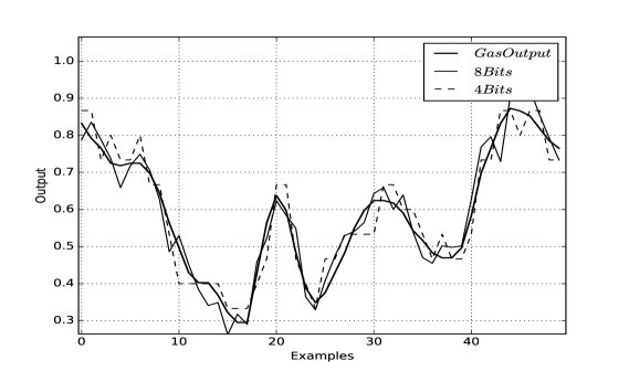
Figure 3: Modeling the gas furnace using conditional probability and binary encoding.

Finally, we test the continuous valued algorithm. We use the simulation model (43). The training parameters are $k_{G}=1,$ $\eta_{1}=0.01,$ and $100$ training epochs for each RBM. For the output layer, the coded features have $k_{G}=1,$ and $10$ training epochs. The testing MSE is $12.5\times 10^{-3}.$ It is better than binary encoding, because it provides more information on real axis.

Wiener-Hammerstein system

Wiener-Hammerstein system [27] has a static nonlinear part surrounded by two dynamic linear systems. There are $188,000$ input/output pairs, defined $u(k)$ and $y\left(k\right)$. We use $100,000$ samples for training, $88,000$ samples for testing. This is a big data modelling problem.

We use the simulation model (43) to compare these models, with $n_{u}=15,$ $n_{y}=0.$ We only show the feature extraction of the proposed method. The random search method uses the RBM number as $20\geq l\geq 2,$ and the hidden node number as $70\geq p\geq 10.$ Then RBM number $l=5,$ the hidden node number $p=50.$ The RBMs are trained using the Gibbs sampling, $k_{G}=1$, the learning rates are $0.01$. It has $10$ training epochs. We use the same structure for the MLP, five hidden layers, each layer has $50$ nodes.

Table 6 shows the testing errors of different methods for the simulation model (43).

56.0343.0148.0135.7112.70\begin{array}[c]{c}\text{Table 6. MSE of different simulation models }\left(\times 10^{-3}\right)\\ \begin{tabular}[c]{|c|c|c|c|c|}\hline\cr MLP&SVM-L&SVM-P&SVM-R&RBM-C\\ \hline\cr$56.03$&$43.01$&$48.01$&$35.71$&$12.70$\\ \hline\cr\end{tabular}\end{array}

MLPSVM-LSVM-PSVM-RRBM-C

We can see that even for the best result obtained by the SVM-R, RBM-C is much better than the others when the input to the models is only control $u(k).$

Now we show how does the training data seize affect the conditional probability modelling. The stochastic gradient descent is a batch process. The $100,000$ training samples are divided into several packages. All packages have the same size. The package seizes are selected as $500,$ $1,000$ and $5,000.$ The probability distributions are calculated with: binary encoding, in the interval $[0,\infty),$ in the interval $[0,1),$ and in the interval $[-\delta,\delta].$

We can see that the RBMs cannot model the probability distribution properly with small batch number, for example $60$ batches. The training error with the size $500$ is little bigger than the size $1,000.$ The fluctuations of the training error with the size $5,000$ vanish, and the interval $[-\delta,\delta]$ becomes unstable. So large batch seize may affect the distributions by some mislead samples.

6 Conclusions

In this paper, the conditional probability based method is applied for nonlinear system modelling. We show that this method is better than the other data based models when there are noises and the previous outputs are not available on-line. The modelling accuracy is satisfied with the binary encoding and continuous values by the modified RBMs. The training algorithms are obtained from maximizing the conditional likelihood of the data set. Two nonlinear modelling problems are used to validate the proposed methods. The simulation results show that the modelling accuracies are improved a lot when there are noises and the simulation models have to be used.

References

• [1] L.Ljung,Β System Identification-Theory for User, Prentice Hall, Englewood Cliffs, NJ 07632, 1987.
• [2] G.Pillonetto, F.Dinuzzo, T.Chenc, G.De Nicolao, L.Ljung, Kernel methods in system identification, machine learning and function estimation: A survey, Automatica, Vol.50, 657-682, 2014
• [3] A.Juloski, S.Weiland, W.Heemels, A Bayesian Approach to Identification of Hybrid Systems, IEEE Transactions on Automatic Control, Vol.50, No.10, 1502-1533, 2005
• [4] Y.Lu, B.Huang, S.Khatibisepehr, Variational Bayesian Approach to Robust Identification of Switched ARX Models, IEEE Transactions on Cybernetics, Vol.46, No.12, 3195-3208, 2016
• [5] T.B.Schona, A.Wills, B.Ninness, System identification of nonlinear state-space models, Automatica, Vol.47, 39-49, 2011
• [6] D.Erhan, Y.Bengio, A.Courville, P-A.Manzagol, P.Vincent, Why Does Unsupervised Pre-training Help Deep Learning?, Journal of Machine Learning Research, vol.11, 625-660, 2010
• [7] P.Damien, P.Dellaportas, N.Polson, D.Stephens, Bayesian Theory and Applications, Oxford University Press, 2015
• [8] A.Fisher, C.Igel, Training restricted Boltzmann machines: an introduction, Pattern Recognition, Vol.4, No.1, 25-39, 2013
• [9] G. E. Hinton, Learning distributed representations of concepts, 8th Annual Conference of the Cognitive Science Society, pp. 1-12, Hillsdale, 1986.
• [10] Y. Bengio, P. Lamblin, D. Popovici, and H. Larochelle, Greedy layer-wise training of deep networks, Advances in Neural Information Processing Systems (NIPS’06), pp. 153-160, MIT Press, 2007.
• [11] G. E. Hinton and T. J. Sejnowski, Learning and relearning in Boltzmann machines, Parallel Distributed Processing: Explorations in the Microstructure of Cognition. Volume 1: Foundations, pp. 282-317, Cambridge, MA: MIT Press, 1986.
• [12] L. Qiu, L. Zhang, Y. Ren, P.N. Suganthan, G. Amaratunga, Ensemble deep learning for regression and time series forecasting, 2014 IEEE Symposium on Computational Intelligence in Ensemble Learning (CIEL), pp.1-6, Orlando, FL, USA , 2014
• [13] E. Busseti, I. Osband, and S. Wong. Deep learning for time series modeling. Technical report, Stanford University, 2012.
• [14] M. LΓ€ngkvist, L. Karlsson, and A. Loutfi. A review of unsupervised feature learning and deep learning for time-series modeling. Pattern Recognition Letters 42: 11-24. 2014.
• [15] V.Nair, G.E. Hinton, Rectified Linear Units Improve Restricted Boltzmann Machines, 27th International Conference on Machine Learning, Haifa, Israel, 2010.
• [16] P. Romeu, et al. Time-Series Forecasting of Indoor Temperature Using Pre-trained Deep Neural Networks. Artificial Neural Networks and Machine Learning–ICANN 2013. Springer Berlin Heidelberg, 451-458. 2013.
• [17] C.Shang, F.Yang, D.Huang, W.Lyu, Data-driven soft sensor development based on deep learning technique, Journal of Process Control, 24, 223–233, 2014
• [18] E. de la Rosa and W. Yu, Randomized algorithms for nonlinear system identification with deep learning modification, Information Sciences, Vol.364, 197-212, 2016
• [19] E. de la Rosa and W.Yu, Restricted Boltzmann machine for nonlinear system modeling, 14th IEEE International Conference on Machine Learning and Applications (ICMLA15), Miami, USA, 2015
• [20] S.A.Billings, Nonlinear System Identification: NARMAX Methods in the Time, Frequency, and Spatio-Temporal Domains, Wiley, 2013
• [21] G. E.Hinton, S.Osindero, Y.W.Teh, A fast learning algorithm for deep belief nets, Neural Computation, Vol.18, No.7, 1527-1554, 2006
• [22] N. Le Roux and Y. Bengio, Representational power of restricted Boltzmann machines and deep belief networks, Neural Computation, Vol. 20, 1631-1649, 2008
• [23] G.Cybenko, Approximation by Superposition of Sigmoidal Activation Function, Math.Control, Sig Syst, Vol.2, 303-314, 1989
• [24] G.B. Huang, L.Chen, and C. K.Siew, Universal approximation using incremental constructive feedforward networks with random hidden nodes, IEEE Transactions on Neural Networks, 17(4):879-92, 2006
• [25] G. Box, G. Jenkins, G. Reinsel. Time Series Analysis: Forecasting and Control, 4th Ed, Wiley, 2008.
• [26] J. Bergstra, Y. Bengio, Random Search for Hyper-Parameter Optimization, Journal of Machine Learning Research, pp 281-305, 2011
• [27] J. Schoukens, J. Suykens, L. Ljung, Wiener-Hammerstein benchmark, 15th IFAC Symposiumon System Identification, Saint-Malo, France, 2009.