Structured Actor-Critic for Managing Public Health Points-of-Dispensing

Abstract

Public health organizations face the problem of dispensing treatments (i.e., vaccines, antibiotics, and others) to groups of affected populations through “points-of-dispensing” (PODs) during emergency situations, typically in the presence of complexities like demand stochasticity, heterogenous utilities (e.g., for vaccine distribution, certain segments of the population may need to be prioritized), and limited storage. We formulate a hierarchical Markov decision process (MDP) model with two levels of decisions (and decision-makers): the upper-level decisions come from an inventory planner that “controls” a lower-level dynamic problem, which optimizes dispensing decisions that take into consideration the heterogeneous utility functions of the random set of PODs. We then derive structural properties of the MDP model and propose an approximate dynamic programming (ADP) algorithm that leverages structure in both the policy and the value space (state-dependent basestocks and concavity, respectively). The algorithm can be considered an actor-critic method; to our knowledge, this paper is the first to jointly exploit policy and value structure within an actor-critic framework. We prove that the policy and value function approximations each converge to their optimal counterparts with probability one and provide a comprehensive numerical analysis showing improved empirical convergence rates when compared to other ADP techniques. Finally, we show how an aggregation-based version of our algorithm can be applied in a realistic case study for the problem of dispensing naloxone (an overdose reversal drug) via first responders amidst the ongoing opioid crisis.

Keywords: public health, actor critic, approximate dynamic programming

Introduction

Public health organizations manage “points-of-dispensing” (PODs), operated by first responders or first receivers (Ablah et al., 2010), for distributing critical medical supplies during emergency situations (e.g., the ongoing opioid crisis, the COVID-19 pandemic, the 2009 H1N1 influenza pandemic, meningitis outbreaks). In this paper, we consider the hierarchical and sequential problem of optimizing inventory control and making dispensing decisions for multiple PODs. Our problem setting is specifically motivated by the ongoing opioid overdose harm reduction efforts of public health organizations in cities across the U.S., where the opioid epidemic was declared a public health emergency in 2017. In particular, our modeling is motivated by the Naloxone for First Responders Program (NFRP), a statewide naloxone distribution initiative in Pennsylvania.

Our setup contains hierarchical decisions in order to model the interplay between two decision-makers: the “upper-level” central inventory manager and a “lower-level” dispensing coordinator. The NFRP is an example of an organization that operates in this manner through the use of a centralized coordinating entity (CCE) that manages dispensing. Both decision-makers make sequential and non-myopic decisions (at different timescales) and are modeled using Markov decision processes (MDPs). Another novel point of emphasis for our model is the notion that the effectiveness of the public health intervention can vary across different groups of the affected population (Lee et al., 2015; Bennett et al., 2018) and across different locations. Therefore, instead of modeling demand in a static and homogeneous manner, we consider the case where at each period, new demand information is revealed sequentially as a POD attribute and demand. The dispensing decisions are made according to the arrivals of PODs with a goal of maximizing total utility. The essential trade-off considered by the dispensing coordinator is: should we satisfy a lower-priority demand now, or save the inventory for a possible higher-priority demand in the future?

The model we develop in this paper, however, is quite general and useful for related problems in public health as well where hierarchical decisions and demand heterogeneity may be an issue (e.g., vaccine distribution, where certain segments of the population are more susceptible and where higher-level inventory and lower-level dispensing decisions might be made separately). Other important characteristics of this problem include demand nonstationarity and the potential for limited storage capacity.

Exact computation of the optimal policy for this model is difficult when the number of states is large, when the stochastic models are unknown, or when demand data is collected slowly over time. The main methodological contribution of the paper addresses these issues through a structured actor-critic algorithm; our proposed method exploits structure in both the policy and the value function and can discover near-optimal policies in a fully data-driven way. Our algorithm uses several gradient updates on each iteration and thus is highly suitable for the situation where data arrives in an ongoing fashion and online updates are desired. In other words, a large batch of historical data is not required for our algorithm and the policy can be learned over time. We now give five examples of public health problems for which our model and algorithm are applicable.

Example 1 (Opioid Overdose Epidemic).

The rate of opioid overdose deaths tripled between 2000 and 2014 in the United States (Rudd et al., 2016). More recently, in July 2017, it was estimated that there are 142 American deaths each day due to overdose (Christie et al., 2017). Naloxone is a drug that has the ability to reverse overdoses within seconds to minutes. To save lives amidst the current opioid epidemic, it is critical for naloxone to be widely distributed. Indeed, many harm reduction programs such as NFRP are undertaking the challenge by distributing naloxone free of charge to first responders. The NFRP program is run by Pennsylvania Commission on Crime and Delinquency (PCCD), who dispenses naloxone to eligible first responders through centralized, local hubs in each county or region First responders include emergency medical services, law enforcement, fire fighters, public transit drivers and so on. One challenge facing these organizations is that the utility of naloxone varies across different types of first responders. Goodloe and Dailey (2014); Rando et al. (2015) emphasize the importance of law enforcement officers, who are “often a community’s first contact with opioid overdose victims after 9-1-1 services have been summoned.” The utility of naloxone also varies across regions due to the varying levels of opioid usage in different populations. The West Virginia Department of Health and Human Resources (DHHR) purchased about 34,000 doses of naloxone; in addition to distributing to the state police, fire departments, and emergency medical services, DHHR additionally planned to distribute 1,000 doses of naloxone to each of the eight high priority counties, including Berkeley, Cabell, Harrison, Kanawha, Mercer, Monongalia, Ohio, and Raleigh (West Virginia DHHR, 2018). Therefore, the prioritization of certain “demand classes” is an important consideration when naloxone is expensive or when quantities are limited; see, e.g., Cohn (2017) for a report on rationing practices in Baltimore.

Example 2 (COVID-19).

By the end of February 2021, COVID-19 has resulted in 28,409,727 cases and 511,903 deaths (CDC, 2021c). Compared with 5-17 age group, the rate of death is 1100 times higher in 65-74 age group, 2800 times higher in 75-84 age group, and 7900 times higher in 85 and older age group (CDC, 2021b). According to the COVID-19 vaccination recommendations by CDC (CDC, 2021a), in phase 1a, healthcare personnel and long-term care facility residents are offered vaccination first. After that, the 75 and older age group and the 65-74 age group are vaccinated in phases 1b and 1c.

Example 3 (Influenza).

The need for distinct demand classes was also observed for the case of vaccine distribution during the 2009 H1N1 influenza pandemic. The H1N1 influenza virus first emerged in Mexico and California in April 2009 (Neumann et al., 2009) and the pandemic lasted until August 2010 (World Health Organization, 2010). Children and young adults were disproportionately affected when compared to older adults (Kwan-Gett et al., 2009): during April 15 and May 5, 2009, among the 642 confirmed infected patients in the U.S. (ranging from 3 months to 81 years old), 60% were 18 years old or younger (H1N1 Virus Investigation Team, 2009). The reported H1N1 cases from April 15 to July 24, 2009, show that the infected rate (number of cases per 100,000 population) of 0 to 4 age group is 17.6 times of the infected rate of 65 and older age group, and the rate of 5 to 24 age group is 20.5 times of the rate of 65 and older age group (CDC, 2009a). The Advisory Committee on Immunization Practice (ACIP) recommended a priority group (about 159 million Americans), in which there was a subset with highest priority (about 62 million Americans) (Rambhia et al., 2010). Patients aged 65 and older were only considered for vaccination once the demand amongst younger groups were met (CDC, 2009b).

Example 4 (Hepatitis A).

Hepatitis A outbreaks began in 2016 and are currently (as of August 2019) ongoing in 29 states across the U.S (CDC, 2019). Recent data from August 16, 2019 shows 4837 cases (60 deaths) in Kentucky, 3244 cases (15 deaths) in Ohio, 2740 cases (31 deaths) in Florida, 918 cases (28 deaths) in Michigan, 2540 cases (23 deaths) in West Virginia, and 2219 cases (13 deaths) in Tennessee (; ; ; ; ; ). This outbreak largely affects the homeless, drug users, and their direct contacts (CDC, 2019). Center for Disease Control (CDC) guidelines suggest that vaccine inventory be conducted monthly to ensure adequate supplies and that the vaccine order decisions take into account projected demand and storage capacity (U.S. HHS and CDC, 2018), two important aspects of our model. The CDC also recommends against overstocking, which presents the risk of wastage and outdated vaccines.

Example 5 (Vaccines for Children Program).

The measles epidemic in 1989 to 1991 revealed the issue of low vaccination rates among children (CDC, 2014). Vaccines for Children (VFC) is a program started in 1994 that aims to reduce the economic barriers of vaccination for disadvantaged children (Santoli et al., 1999; Zimmerman et al., 2001; Smith et al., 2005). It supplies free vaccines (including influenza, hepatitis A, hepatitis B, and measles) to registered providers, who in turn provide vaccinations to eligible children (Zimmerman et al., 2001; Social Security Online, 2005). Before healthcare providers are enrolled, VFC coordinators perform site visits to ensure proper storage practice (CDC, 2012). A study in 2012 found, however, that out of 45 VFC providers, 76% exposed VFC vaccines to inappropriate temperatures, and 16% kept expired VFC vaccines (Levinson, 2012).

Our Results.

The main contributions of this paper are summarized below.

• In this paper, we first develop and analyze a hierarchical, finite-horizon Markov decision process (MDP) model that abstracts the above problems into a single framework. The upper-level problem (the “upper-level MDP”) is an inventory model that controls a lower-level dispensing problem (the “lower-level MDP”). Here, we consider the setting where the utilities of PODs differ across regions due to the varying intervention effects on patients in different populations. The demand and POD-attribute distributions at each period depend on an information process, which can represent past demand realizations or other external information.

• We then analyze the structural properties of the model. The MDP features basestock-like structure in a discrete state setting and discretely-concave value functions; both of these properties depend on the discrete-concavity observed in the lower-level problem. The motivation for a discrete state formulation comes from the naloxone distribution application, where demand quantities are relatively small; this is not an ideal setting for use of a continuous state approximation.

• Next, we propose a new actor-critic algorithm (Sutton and Barto, 1998; Konda and Tsitsiklis, 2000) that exploits the structural properties of the MDP. More specifically, the algorithm tracks both policy and value function approximations (an identifying feature of an “actor-critic” method) and utilizes the structure to improve the empirical convergence rate. Moreover, the algorithm is suited for a setting where data arrive continually and the policy is updated over time. This algorithm (and its general idea) is potentially of broader interest, beyond the public health application.

• Finally, we present a case study for the problem of dispensing naloxone. We show how an aggregation-based version of the algorithm can be applied in a setting with continuous information states. In addition to computing approximations to the optimal inventory management and dispensing strategies, we also conduct a sensitivity analysis to understand the impact of various model parameters.

The paper is organized as follows. A literature review is provided in Section 2. We introduce the hierarchical MDP model in Section 3 and derive its structural properties in Section 4. The proposed stuctured actor-critic algorithm is given and discussed in Section 5. In Section 6, we conduct numerical experiments. We propose an aggregation-based version of the algorithm in Section C and finally present the naloxone case study in Section 7.

Literature Review

In this section, we provide a brief review of related literature. The upper-level replenishment decisions in this paper are closely related to both lost-sales and perishable inventory models. In the lost-sales case, Nahmias (1979) constructs simple myopic approximations for three variations of the classical model with lead time. Ha (1997) studies a single-item, make-to-stock production model with several demand classes and lost sales and constructs stock-rationing levels for the optimal policy. Mohebbi (2003) focuses on random supply interruptions in lost-sales inventory systems with positive lead times. Zipkin (2008a) finds that the standard base-stock policy performs poorly compared to some other heuristic policies. We also refer readers to Bijvank and Vis (2011) for a detailed review. Our public health application is also somewhat related to the problems studied in perishable inventory models (Janssen et al., 2016), even though our motivating application does not require us to explicitly model age.

Related to our hierarchical model is the case of multi-echelon systems, where, for example, an upper echelon (e.g. a central warehouse) replenishes the inventory of a lower echelon (e.g. a retailer) that serves demand (Clark and Scarf, 1960). Tan (1974) studies the optimal ordering and allocation policies for the upper echelon and Graves (1996) constructs an allocation policy for the multi-echelon system. In the model of Chen and Samroengraja (2000), each retailer is allowed to replenish once from the warehouse during an ordering cycle. Van Houtum et al. (2007) shows the optimality of base-stock policies and derives newsvendor-type equations for the optimal base-stock levels. Zhou et al. (2013) studies a multi-product multi-echelon inventory system. Grob (2018) aims to optimize the reorder points of both echelons given fixed order quantities. Our model expands upon this literature in that the optimization problems for the two echelons are modeled as two nested MDPs (or a “hierarchical” MDP). We show the concavity of the value function of both the upper-level and lower-level, which is then utilized to derive the structured actor-critic algorithm.

Our proposed actor-critic method falls under the class of approximate dynamic programming (ADP) or reinforcement learning (RL) algorithms (Bertsekas and Tsitsiklis, 1996; Sutton and Barto, 1998; Powell, 2007). Possibly the most well-known RL technique is Q-learning (Watkins, 1989), a model-free approach that uses stochastic approximation (SA) to learn state-action value function (or “Q-function”). In some cases, convexity of the value function is known a priori and can be exploited; see, e.g., Pereira and Pinto (1991); Powell et al. (2004); Nascimento and Powell (2009); Philpott and Guan (2008); Shapiro (2011); Löhndorf et al. (2013). The updates used in the value function approximation part of our algorithm most closely resembles Powell et al. (2004) and Nascimento and Powell (2009).

Related to the policy function approximation part of our algorithm, Kunnumkal and Topaloglu (2008) proposes a stochastic approximation method to compute basestock levels in continuous state inventory problems. Our method also utilizes two types of basestock structure, but it does so in a different way from Kunnumkal and Topaloglu (2008) due to our focus on discrete-valued inventory states. The primary feature of an actor-critic algorithm is that it approximates both the policy and value function (Werbos, 1974; Witten, 1977; Werbos, 1992; Konda and Tsitsiklis, 2000). The “actor” is the policy function approximation (for selecting actions) and the “critic” represents the value function approximation used to “criticize” the actions selected by the actor. The novelty of our method is due to its use of the structure in both the value function and the policy. Our experimental results show significant advantages of exploiting this policy-value structure. Further, differing from most actor-critic methods, we do not use stochastic policy, reducing the number of policy parameters to be learned.

In addition, state aggregation is a commonly used method to deal with large dynamic problems (Fox, 1973; Bean et al., 1987; Singh et al., 1995), including inventory management (Schweitzer et al., 1985; Chen et al., 1999; Chen, 1999; Mousavi et al., 2004; Zaher and Zaki, 2014). Error bounds for these types of approximations can be found in Bertsekas (1975), Ren and Krogh (2002), and Van Roy (2006). Our results in Section 7 make use of partial aggregation of the state space.

Due to the discrete inventory states used in our model, we make use of the concept of $L^{\natural}$-convexity (concavity) as a tool in the analysis. This theory was first developed in Fujishige and Murota (2000) for discrete convex analysis and then extended to continuous variables by Murota and Shioura (2000). Closely related concepts are $l$-convexity and submodularity. It turns out that these ideas are useful in understanding the structures of optimal policies in the field of inventory management, as introduced by Lu and Song (2005) in an assemble-to-order multi-item system. Zipkin (2008b) uses $L^{\natural}$-convexity in some variations of the basic multiperiod lost-sales model with lead time and Huh and Janakiraman (2010) extend the results to lost-sales serial inventory systems. Pang et al. (2012) use similar ideas to analyze inventory-pricing systems with lead time, and Gong and Chao (2013) study finite capacity systems with both manufacturing and remanufacturing. See Xin (2017) for a survey of applications utilizing the theory of $L^{\natural}$-convexity.

As for the utility in our model, the quality-adjusted life-year (QALY) is widely used to in healthcare to measure the value of medical interventions. The QALY was originally developed for cost-effectiveness analysis to decide scarce resource allocation across competing healthcare programs (Fanshel and Bush, 1970; Torrance et al., 1972; Weinstein and Stason, 1977), and has been endorsed by the US Panel on Cost-Effectiveness in Health and Medicine as a standardized methodological approach in cost-effectiveness analyses (Weinstein et al., 1996). The QALY has been used in naloxone distribution research to evaluate the cost-effectiveness of distributing naloxone to heroin users (Coffin and Sullivan, 2013), distributing naloxone to adults at risk of heroin overdose in UK (Langham et al., 2018), and one-time versus biannual distribution (Acharya et al., 2020).

Model Formulation

As discussed above, our MDP model is motivated by the hierarchical structure of public health organizations, such as Pennsylvania’s NFRP, which distributes naloxone to a CCE that, in turn, coordinates the dispensing of naloxone to first responders in various counties. We assume that the central inventory manager makes replenish-up-to and dispense-down-to decisions to the central storage periodically. Then, naloxone is distributed to the dispensing coordinator, who makes dispensing decisions to sequentially and randomly arriving PODs. Given an initial allotment of inventory, the dispensing decisions to PODs are made with the goal of maximizing cumulative utility of the satisfied naloxone demand within the dispensing period. The timing of events during each period is as follows: (1) the central inventory manager decides the replenish-up-to and dispense-down-to levels, (2) the dispensing coordinator receives naloxone, and (3) based on POD demands, POD attributes, and the level of available inventory, the dispensing coordinator dispenses naloxone in order to maximize utility. Figure 1 gives an illustration of the timing of these events. In this section, we first discuss the lower-level dispensing problem and then illustrate the upper-level inventory control model.

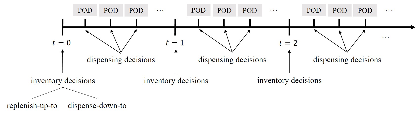
Figure 1: Sequence of Events

The Dispensing MDP

We first discuss the lower-level MDP for making dispensing decisions within each period $t$. After the central inventory manager makes the replenish-up-to and dispense-down-to decisions, the dispensing coordinator receives a sequence of POD demands to satisfy, starting with an initial inventory allotment based on the dispense-down-to decision. The dispensing model contains $n$ sub-periods. In sub-period $i$, the arriving POD is represented by an attribute $\Xi_{t,i}$ which is interpreted as the arriving POD’s attributes. When there is no arriving POD in sub-period i, $\Xi_{t,i}=0$. The distribution of $\Xi_{t,i}$ depends on an exogenous information process $\{W_{t}\}$ that transitions according to the upper-level timescale (and thus stays fixed at a particular realization $w$ for all sub-periods in the dispensing problem; a full description of this process will be given in Section 3.2). Given realizations $w_{t}$ and $\xi_{t,i}$ of the exogenous information $W_{t}$ and attribute $\Xi_{t,i}$, we consider an increasing expected utility function $u_{w_{t}}(\cdot,\xi_{t,i})$, whose argument is the number of inventory units $y_{i}$ dispensed to the arriving POD in sub-period $i$. For the remainder of this section, we omit the subscript $t$ in for convenience.

These utility functions should be interpreted as parameters specified by the public health organization. The motivation for modeling heterogeneous utilties for the case of naloxone dispensing is primarily due to varying severity of the epidemic across different regions and populations (first responders in regions with more opioid users should have higher priority). To model this heterogeneity in demand, our model allows region and other related information to be encoded within the attribute $\xi_{i}$, which then determines the utility.

The dispensing coordinator aims to maximize the total utility subject to the initial inventory allotment $x_{0}$. In sub-period $i$, given exogenous information $w$, available inventory level $x_{i}$ and attribute state $\xi_{i}$ about the arriving POD, a dispensing decision $y_{i}$ is made. Let $\{\mu_{w,0},\mu_{w,1},\ldots,\mu_{w,n-1}\}$ be lower-level dispensing policy for exogenous information $w$ and suppose $\mathcal{M}_{w}$ is the set of all feasible policies that satisfy $\mu_{w,i}(x_{i},\xi_{i})\leq x_{i}$. The objective on the lower-level is given by

$$U_{w,0}(x_{0},\xi_{0})=\max_{\mu_{w}\in\mathcal{M}_{w}}\mathbf{E}\left[\sum_{i=0}^{n-1}u_{w}\bigl{(}\mu_{w,i}(X_{i},\Xi_{i}),\Xi_{i}\bigr{)}\,\Bigl{|}\,X_{0}=x_{0},\Xi_{0}=\xi_{0},W=w\right],$$

where the transition follows $X_{i+1}=x_{i}-\mu_{w,i}(x_{i},\xi_{i})$. The optimum is attained by an optimal policy $\mu^{*}_{w}$. We now write the Bellman optimality equation for the objective:

$$\textstyle U_{w,i}(x_{i},\xi_{i})=\textnormal{max}_{y_{i}\leq x_{i}}\;u_{w}\bigl{(}y_{i},\xi_{i}\bigr{)}+\mathbf{E}_{w}\bigl{[}U_{w,i+1}(X_{i+1},\Xi_{i+1})\bigr{]}$$ (1)

for $i=0,1,\ldots,n-1$, and $U_{w,n}(x_{n},\xi_{n})=0$, where $\mathbf{E}_{w}$ is being used as shorthand for the expected value conditioned on $\{W_{t}=w\}$.

The Inventory Control MDP

The sequential inventory control aspect of the model contains $T$ planning periods. In each period, there are two decisions to be made: the replenish-up-to level and the dispense-down-to level. In the first period $t=0$, the initial resource level $R_{0}=0$. In the last period $t=T$, no decision is made and the remaining inventory $R_{T}$ is either worthless or charged a disposal cost (controlled by a parameter $b\geq 0$). Let $\{W_{t}\}$ be the aforementioned exogenous information process, which may contain information regarding past POD demands, current disease trends, or other dynamic information related to the public health situation. As discussed above, the information state $W_{t}$ influences the distribution of the attributes $\Xi_{t,i}$ of the arriving PODs for sub-periods $i=1,2,\ldots,n$ of the lower-level problem in period $t$. We assume that $W_{t}$ takes values in a finite set $\mathcal{W}$ and that it is a Markov process.

Let $R_{\textnormal{max}}$ be the capacity of the central storage facility. At the end of each period $t$, the central inventory manager makes a replenish-up-to decision $z^{\textnormal{rep}}_{t}$ based on the available resource level $R_{t}\in\{0,1,\ldots,R_{\textnormal{max}}\}$ and the exogenous information $W_{t}\in\mathcal{W}$. After this, the central inventory manager makes a dispense-down-to decision $z^{\textnormal{dis}}_{t}$ based on the replenish-up-to decision $z^{\textnormal{rep}}_{t}$ and $W_{t}$.

We will often refer to particular values of the resource level $R_{t}$ and exogenous information $W_{t}$ using the notations $r$ and $w$, respectively. Let $\bar{\mathcal{Z}}(r)=\{r,r+1,\ldots,R_{\textnormal{max}}\}$ be the set of feasible replenish-up-to decisions if the current inventory level is $r$, so that $z^{\textnormal{rep}}_{t}\in\bar{\mathcal{Z}}(R_{t})$ in period $t$. This means the central inventory manager orders $z^{\textnormal{rep}}_{t}-R_{t}$ units of inventory with a per-unit ordering cost $c_{w}\geq c_{\textnormal{min}}$ (note that we allow this ordering cost to depend on the exogenous information $w$), where $c_{\textnormal{min}}$ is a positive scalar.

Let $\underline{\mathcal{Z}}(z^{\textnormal{rep}})=\{0,1,\ldots,z^{\textnormal{rep}}\}$ be the set of feasible dispense-down-to decisions if the current resource level is $z^{\textnormal{rep}}$, so that $z^{\textnormal{dis}}_{t}\in\underline{\mathcal{Z}}(z^{\textnormal{rep}}_{t})$ in period $t$. This means the central inventory manager delivers $z^{\textnormal{rep}}_{t}-z^{\textnormal{dis}}_{t}$ units of inventory to the dispensing coordinator, and $z^{\textnormal{rep}}_{t}-z^{\textnormal{dis}}_{t}$ serves as the initial inventory allotment in the lower-level dispensing MDP problem. The transition to the next inventory state $R_{t+1}$ is given by:

$$\textstyle R_{t+1}=z^{\textnormal{dis}}_{t}.$$ (2)

Each unit of leftover inventory after applying the transition (2) is charged a holding cost $h<c_{\textnormal{min}}$.

A policy $\{\pi_{0},\pi_{1},\ldots,\pi_{T-1}\}$ is a sequence of mappings $\pi_{t}=(\pi_{t}^{\textnormal{rep}},\pi_{t}^{\textnormal{dis}})$ from states $(R_{t},W_{t})$ to replenish-up-to levels and dispense-down-to levels. Let $\Pi$ be the set of all feasible policies that satisfy $\pi_{t}^{\textnormal{rep}}(R_{t},W_{t})\geq R_{t}$ and $\pi_{t}^{\textnormal{dis}}(R_{t},W_{t})\leq\pi_{t}^{\textnormal{rep}}(R_{t},W_{t})$. Our objective is given by:

$$\max_{\pi\in\Pi}\;\mathbf{E}\Biggl{[}\sum_{t=0}^{T-1}\bigl{(}-hR_{t}-c_{W_{t}}\bigl{(}\pi_{t}^{\textnormal{rep}}(R_{t},W_{t})-R_{t}\bigr{)}+U_{W_{t},0}\bigl{(}\pi_{t}^{\textnormal{rep}}(R_{t},W_{t})-\pi_{t}^{\textnormal{dis}}(R_{t},W_{t}),\,\Xi_{t,0}\bigr{)}\Biggr{]}-b\,R_{T},$$

where $R_{t}$ transitions according to (2) for $(z^{\textnormal{rep}}_{t},z^{\textnormal{dis}}_{t})=\pi_{t}(R_{t},W_{t})$, and the gap between the two decisions of the upper-level problem, $\pi_{t}^{\textnormal{rep}}(R_{t},W_{t})-\pi_{t}^{\textnormal{dis}}(R_{t},W_{t})$, serves as the initial resource level of the lower-level problem. We now write a preliminary set of Bellman optimality equations for the objective above. Let $V_{T}(r,w)=-b\,r$ be the terminal value (note: $b$ is zero if there is no disposal cost). For $t<T$, we have

$$V_{t}(r,w)=\max_{z^{\textnormal{rep}}\in\bar{\mathcal{Z}}(r),z^{\textnormal{dis}}\in\underline{\mathcal{Z}}(z^{\textnormal{rep}})} (c_{w}-h)\,r-c_{w}z^{\textnormal{rep}}+\mathbf{E}_{w}\bigl{[}U_{w,0}\bigl{(}z^{\textnormal{rep}}-z^{\textnormal{dis}},\Xi_{t,0}\bigr{)}+V_{t+1}\bigl{(}z^{\textnormal{dis}},W_{t+1}\bigr{)}\bigr{]}.$$ (3)

So far, we have considered $z^{\textnormal{rep}}$ and $z^{\textnormal{dis}}$ as being made simultaneously in each period, but we can equivalently view the dispense-down-to decision $z^{\textnormal{dis}}$ to be taken after the replenish-up-to decision $z^{\textnormal{rep}}$ (this reflects the reality and also is useful for our analysis and algorithm). The set $\underline{\mathcal{Z}}(z^{\textnormal{rep}})$ of feasible dispense-down-to decisions is dependent on the replenish-up-to decision $z^{\textnormal{rep}}$. Therefore, the value function in each period can be broken into two steps:

$$\textstyle V_{t}^{\textnormal{rep}}(r,w)=(c_{w}-h)\,r+\max_{z^{\textnormal{rep}}\in\bar{\mathcal{Z}}(r)}\bigl{\{}-c_{w}z^{\textnormal{rep}}+V_{t}^{\textnormal{dis}}(z^{\textnormal{rep}},w)\bigr{\}},$$ (4)

$$\textstyle V_{t}^{\textnormal{dis}}(z^{\textnormal{rep}},w)=\max_{z^{\textnormal{dis}}\in\underline{\mathcal{Z}}(z^{\textnormal{rep}})}\mathbf{E}_{w}\bigl{[}U_{w,0}\bigl{(}z^{\textnormal{rep}}-z^{\textnormal{dis}},\Xi_{t,0}\bigr{)}+V_{t+1}^{\textnormal{rep}}\bigl{(}z^{\textnormal{dis}},W_{t+1}\bigr{)}\bigr{]},$$ (5)

with $V_{T}^{\textnormal{rep}}(r,w)=-b\,r$. Similarly, there are two postdecision value functions in each period corresponding to the replenish-up-to decision and the dispense-down-to decision respectively:

$$\textstyle\tilde{V}_{t}^{\textnormal{rep}}(z^{\textnormal{rep}},w)=-c_{w}z^{\textnormal{rep}}+V_{t}^{\textnormal{dis}}(z^{\textnormal{rep}},w),$$ (6)

$$\textstyle\tilde{V}_{t}^{\textnormal{dis}}(z^{\textnormal{dis}},w)=\mathbf{E}_{w}\bigl{[}V_{t+1}^{\textnormal{rep}}\bigl{(}z^{\textnormal{dis}},W_{t+1}\bigr{)}\bigr{]}.$$ (7)

The optimal policy can be written as follows

$$\textstyle\pi_{t}^{\textnormal{rep},*}(r,w)\in\operatorname*{arg\,max}_{z^{\textnormal{rep}}\in\bar{\mathcal{Z}}(r)}\;\tilde{V}_{t}^{\textnormal{rep}}(z^{\textnormal{rep}},w).$$ (8)

$$\textstyle\pi_{t}^{\textnormal{dis},*}(z^{\textnormal{rep}},w)\in\operatorname*{arg\,max}_{z^{\textnormal{dis}}\in\underline{\mathcal{Z}}(z^{\textnormal{rep}})}\;\mathbf{E}_{w}\bigl{[}U_{w,0}\bigl{(}z^{\textnormal{rep}}-z^{\textnormal{dis}},\Xi_{t,0}\bigr{)}\bigr{]}+\tilde{V}_{t}^{\textnormal{dis}}(z^{\textnormal{dis}},w),$$ (9)

where, with a slight abuse/reuse of notation, $\pi_{t}^{\textnormal{dis},*}(z^{\textnormal{rep}},w)$ is the optimal dispense-down-to policy when the replenish-up-to level is $z^{\textnormal{rep}}$. Combining (4)-(9), we obtain equivalent formulations of the optimality equation written using $\tilde{V}_{t}^{\textnormal{rep}}(z^{\textnormal{rep}},w)$, $\tilde{V}_{t}^{\textnormal{dis}}(z^{\textnormal{dis}},w)$, $\pi_{t}^{\textnormal{rep},*}(r,w)$, and $\pi_{t}^{\textnormal{dis},*}(z^{\textnormal{rep}},w)$:

$$\textstyle\tilde{V}_{t}^{\textnormal{rep}}(z^{\textnormal{rep}},w)=-c_{w}z^{\textnormal{rep}}+\mathbf{E}_{w}\bigl{[}U_{w,0}\bigl{(}z^{\textnormal{rep}}-\pi_{t}^{\textnormal{dis},*}(z^{\textnormal{rep}},w),\,\Xi_{t,0}\bigr{)}\bigr{]}+\tilde{V}_{t}^{\textnormal{dis}}\bigl{(}\pi_{t}^{\textnormal{dis},*}(z^{\textnormal{rep}},w),w\bigr{)},$$ (10)

$$\textstyle\tilde{V}_{t}^{\textnormal{dis}}(z^{\textnormal{dis}},w)=\mathbf{E}_{w}\bigl{[}(c_{W_{t+1}}-h)\,z^{\textnormal{dis}}+\tilde{V}_{t+1}^{\textnormal{rep}}\bigl{(}\pi_{t+1}^{\textnormal{rep},*}(z^{\textnormal{dis}},W_{t+1}),W_{t+1}\bigr{)}\bigr{]},$$ (11)

with $\textstyle\tilde{V}_{T-1}^{\textnormal{dis}}(z^{\textnormal{dis}},w)=-b\,z^{\textnormal{dis}}$.

Our proposed algorithm will make use of the convenient formulations of $\tilde{V}_{t}^{\textnormal{rep}}(z^{\textnormal{rep}},w)$ and $\tilde{V}_{t}^{\textnormal{dis}}(z^{\textnormal{dis}},w)$ as expectations in (10) and (11). These formulations are useful for ADP for two reasons: (1) the maximization is within the expectation, so a data- or sample-driven method is easier to incorporate and (2) knowledge about the policies $\pi^{\textnormal{rep},*}_{t}$ and $\pi^{\textnormal{dis},*}_{t}$ can be used within a value function approximation procedure. Indeed, our actor-critic algorithm will make use of the interplay between the greedy policy functions (8) and (9) and the optimal value functions (6) and (7).

Structural Properties

In this section, we analyze the structure properties of the postdecision value functions $\tilde{V}_{t}^{\textnormal{rep}}$ and $\tilde{V}_{t}^{\textnormal{dis}}$ and the optimal policies $\pi_{t}^{\textnormal{rep},*}$ and $\pi_{t}^{\textnormal{dis},*}$. We remind the reader that our model uses discrete inventory states. As opposed to the standard continuous inventory state approximation, this modeling decision was made in order to accomodate the public health setting, where resources are potentially scarce. Our structural analysis makes use the properties of $L^{\natural}$-concave functions, an approach used often in inventory models (Xin, 2017).

Definition 1 ($L^{\natural}$-concave function).

A function $g:\mathbb{Z}^{d}\rightarrow\mathbb{R}\cup\{+\infty\}$ with $\text{dom}\,g\neq\emptyset$ is $L^{\natural}$-concave if and only if it satisfies discrete midpoint concavity:

$$g(p)+g(q)\leq g\left(\left\lceil\dfrac{p+q}{2}\right\rceil\right)+g\left(\left\lfloor\dfrac{p+q}{2}\right\rfloor\right)$$ (12)

for all $p,q\in\mathbb{Z}^{d}$, where $\lceil\cdot\rceil$ and $\lfloor\cdot\rfloor$ are the ceiling and floor functions, respectively.

For the one-dimensional case, $g:\mathbb{Z}\rightarrow\mathbb{R}$, the condition (12) can be reduced to the simpler statement: $g(p)-g(p-1)\geq g(p+1)-g(p)$ for all $p\in\mathbb{Z}$, and $L^{\natural}$-concavity is equivalent to discrete concavity (Murota, 1998). Throughout the rest of the paper, we will use discretely concave to refer to one-dimensional functions that satisfy this condition.

Assumption 1.

For any $w$ and $\xi$, the expected utility function $u_{w}(x,\xi)$ is discretely concave in $x$.

Proposition 1.

Suppose Assumption 1 is satisfied. Then, for each information state $w$, POD attribute $\xi$, and sub-period $i$, the lower-level value function $U_{w,i}(x,\xi)$ is discretely concave in the inventory state $x$.

Proposition 2.

Suppose Assumption 1 is satisfied. Then, the following properties hold:

1. For each $t$ and information state $w$, the postdecision value function $\tilde{V}_{t}^{\textnormal{rep}}(z^{\textnormal{rep}},w)$ is discretely concave in $z^{\textnormal{rep}}$ and $\tilde{V}_{t}^{\textnormal{dis}}(z^{\textnormal{dis}},w)$ is discretely concave in $z^{\textnormal{dis}}$.

2. For each $t$ and state $(r,w)$, the optimal policy $\pi_{t}^{\textnormal{rep},*}(r,w)$ can be written as a series of state-dependent, discrete basestock policies, with thresholds $l^{\textnormal{rep}}_{t}(w)\in\{0,1,\ldots,R_{\textnormal{max}}\}$:

   $$\pi_{t}^{\textnormal{rep},*}(r,w)=\max\{r,l^{\textnormal{rep}}_{t}(w)\}.$$

   It is optimal to replenish the inventory level as close as possible to $l^{\textnormal{rep}}_{t}(w)$.

3. For each $t$ and state $(z^{\textnormal{rep}},w)$, the optimal policy $\pi_{t}^{\textnormal{dis},*}(z^{\textnormal{rep}},w)$ can be written as a series of state-dependent, discrete basestock policies, with thresholds $l^{\textnormal{dis}}_{t}(z^{\textnormal{rep}},w)\in\{0,1,\ldots,R_{\textnormal{max}}\}$:

   $$\pi_{t}^{\textnormal{dis},*}(z^{\textnormal{rep}},w)=\min\{z^{\textnormal{rep}},l^{\textnormal{dis}}_{t}(z^{\textnormal{rep}},w)\}.$$

Proof.

See Appendix A.2 for the proof of Part 1. Parts 2 and 3 then follow directly from (8) and (9) respectively. ∎

We remark that the state-dependency of the replenish-up-to thresholds $l^{\textnormal{rep}}_{t}(w)$ in Proposition 2 refers only to the exogenous information state $W_{t}$, while the dispense-down-to thresholds $l^{\textnormal{dis}}_{t}(z^{\textnormal{rep}},w)$ are dependent on both the inventory and information states $(z^{\textnormal{rep}},w)$. In the former case, if $r<l^{\textnormal{rep}}_{t}(w)$, it is optimal to replenish up to $l^{\textnormal{rep}}_{t}(w)$, while if $r_{t}\geq l^{\textnormal{rep}}_{t}(w)$, it is optimal not to replenish. The quantity ordered is given by $\pi_{t}^{*,\textnormal{rep}}(r,w)-r$. In the latter case, if $z^{\textnormal{rep}}>l^{\textnormal{dis}}_{t}(z^{\textnormal{rep}},w)$, it is optimal to dispense down to $l^{\textnormal{dis}}_{t}(z^{\textnormal{rep}},w)$, while if $z^{\textnormal{rep}}\leq l^{\textnormal{dis}}_{t}(z^{\textnormal{rep}},w)$, it is optimal to dispense down to $z^{\textnormal{rep}}$.

For algorithmic reasons, we define $v^{\textnormal{rep}}_{t}(z^{\textnormal{rep}},w)=\Delta\tilde{V}^{\textnormal{rep}}_{t}(z^{\textnormal{rep}},w)$ and $v^{\textnormal{dis}}_{t}(z^{\textnormal{dis}},w)=\Delta\tilde{V}^{\textnormal{dis}}_{t}(z^{\textnormal{dis}},w)$ to be the “slopes” of postdecision state values $\tilde{V}^{\textnormal{rep}}_{t}(z^{\textnormal{rep}},w)$ and $\tilde{V}^{\textnormal{dis}}_{t}(z^{\textnormal{dis}},w)$ respectively, where $\Delta\tilde{V}^{\textnormal{rep}}_{t}(z^{\textnormal{rep}},w)=\tilde{V}^{\textnormal{rep}}_{t}(z^{\textnormal{rep}},w)-\tilde{V}^{\textnormal{rep}}_{t}(z^{\textnormal{rep}}-1,w)$, $\Delta\tilde{V}^{\textnormal{dis}}_{t}(z^{\textnormal{dis}},w)=\tilde{V}^{\textnormal{dis}}_{t}(z^{\textnormal{dis}},w)-\tilde{V}^{\textnormal{dis}}_{t}(z^{\textnormal{dis}}-1,w)$, and $\tilde{V}^{\textnormal{rep}}_{t}(-1,w)=\tilde{V}^{\textnormal{dis}}_{t}(-1,w)\equiv 0$. It holds that $\tilde{V}^{\textnormal{rep}}_{t}(z^{\textnormal{rep}},w)=\sum_{z^{\prime}=0}^{z^{\textnormal{rep}}}v^{\textnormal{rep}}_{t}(z^{\prime},w)$, where $v^{\textnormal{rep}}_{t}(0,w)\equiv\tilde{V}^{\textnormal{rep}}_{t}(0,w)$. Proposition 2 implies that $v^{\textnormal{rep}}_{t}(z,w)\geq v^{\textnormal{rep}}_{t}(z^{\prime},w)$ for all $0<z\leq z^{\prime}$. The same is true for $\tilde{V}^{\textnormal{dis}}_{t}(z^{\textnormal{dis}},w)$ and $v^{\textnormal{dis}}_{t}(z^{\textnormal{dis}},w)$.

The Structured Actor-Critic Method

In this section, we focus on the upper-level inventory control and dispensing problem and introduce the structured actor-critic (S-AC) algorithm. The goal of the algorithm is to approximate the postdecision value functions $\tilde{V}^{\textnormal{rep}}$ and $\tilde{V}^{\textnormal{dis}}$ and the optimal (basestock) policies $\pi^{\textnormal{rep},*}$ and $\pi^{\textnormal{dis},*}$ by exploiting structure for both. For the lower-level dispensing problem, we use backward induction to solve the dynamic programming exactly, and apply the optimal lower-level dispensing policy $\mu^{*}_{w}$ to each of the arrived PODs.

Overview of the Main Idea

Our algorithm is based on the recursive relationship of (6) and (7) and the properties of the problem as described in Proposition 2. The basic structure is a time-dependent version of the actor-critic method, which makes use of the interaction between the value approximations and the policy approximations in each iteration. The “actor” refers to the policy approxmations $\{\bar{\pi}^{\textnormal{rep},k}\}$ and $\{\bar{\pi}^{\textnormal{dis},k}\}$, and the “critic” refers to the value approximations $\{\bar{V}^{\textnormal{rep},k}\}$ and $\{\bar{V}^{\textnormal{dis},k}\}$. If the optimal policy is known, then the postdecision values can be calculated by (10) and (11); similarly, if the value function is known, the optimal policies can be calculated by (8) and (9). The proposed algorithm applies these two relationships in an alternating fashion.

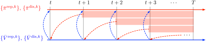
Figure 2: An illustration of how value and policy functions interact under the S-AC algorithm.

We represent the replenish-up-to policy by approximate basestock thresholds $\{\mkern 1.5mu\overline{\mkern-0.5mul\mkern-0.5mu}\mkern 1.5mu^{\textnormal{rep},k}\}$, where $\mkern 1.5mu\overline{\mkern-0.5mul\mkern-0.5mu}\mkern 1.5mu^{\textnormal{rep},k}_{t}(w)$ is the approximation to $l^{\textnormal{rep}}_{t}(w)$ at iteration $k$. Note that compared to a standard actor-critic implementation which tracks a stochastic policy for each state (Sutton and Barto, 1998), this is a significant reduction in the number of parameters needed to be learned. We represent the dispense-down-to policy as approximations $\{\bar{\pi}^{\textnormal{dis},k}_{t}(z^{\textnormal{rep}},w)\}$. As for the values, we represent them as approximations $\{\bar{v}^{\textnormal{rep},k}\}$ and $\{\bar{v}^{\textnormal{dis},k}\}$, where $\bar{v}^{\textnormal{rep},k}_{t}(z^{\textnormal{rep}},w)$ and $\bar{v}^{\textnormal{dis},k}_{t}(z^{\textnormal{dis}},w)$ approximate the discrete slopes $v^{\textnormal{rep}}_{t}(z^{\textnormal{rep}},w)=\Delta\tilde{V}^{\textnormal{rep}}_{t}(z^{\textnormal{rep}},w)$ and $v^{\textnormal{dis}}_{t}(z^{\textnormal{dis}},w)=\Delta\tilde{V}^{\textnormal{dis}}_{t}(z^{\textnormal{dis}},w)$, respectively. According to Proposition 2, if the approximations of the slopes are nonincreasing in $z^{\textnormal{rep}}$ and $z^{\textnormal{dis}}$, respectively, then the approximate value function is discretely concave in each of the decisions.

These approximations are iteratively updated via a stochastic approximation method (Robbins and Monro, 1951; Kushner and Yin, 2003). At each iteration, the algorithm has three steps. In the first step, we observe an exogenous information sequence and the attribute-request vectors for the whole planning horizon. In the second step, we observe the value of the current state under the current policy approximations, subject to the observed attribute-demand vectors. This value is used to update the value approximations. Finally, in the third step, we use the implied basestock threshold from the latest value function to update our approximate policy. The interactions between the policy and value approximations are shown in Figure 2.

Throughout the rest of the paper, we use bar notation (e.g., $\bar{v}^{\textnormal{rep},k}$ or $\mkern 1.5mu\overline{\mkern-0.5mul\mkern-0.5mu}\mkern 1.5mu^{\textnormal{rep},k}$) to denote approximations tracked by the algorithm at iteration $k$. On the other hand, we use hat notation (e.g., $\hat{V}^{\textnormal{rep},k}_{t}$ or $\hat{v}^{\textnormal{rep},k}_{t}$) to denote observed values at iteration $k$ (these are one-time observations used to update the tracked approximations).

Algorithm Description

First, let us give some notation. The observed trajectory of the exogenous information process $\{W_{t}\}$ at iteration $k$ is denoted $\{w_{0}^{k},w_{1}^{k},\ldots,w_{T-1}^{k}\}$ and the initial postdecision replenished resource level at period 0 is $z_{0}^{\textnormal{rep,k}}$. The corresponding attribute $\{\xi_{t,1}^{k}\}$ observed at iteration $k$ is assumed to follow the conditional distributions given $w_{t}^{k}$. Similarly, let $\mathbf{Z}^{k}_{t}(w)$ be an independent realization of the process $(W_{\tau},\xi_{\tau,1})_{\tau=t}^{T-1}$ conditioned on $W_{t}=w$. This sequence of realizations is used to obtain an observation of the value of policy approximation starting at $t$ and $W_{t}=w$ and we denote its elements by

$$\mathbf{Z}^{k}_{t}(w)=\bigl{\{}(\check{w}_{\tau}^{k},\check{\xi}_{\tau,1}^{k}):\tau=t,\ldots,T-1\bigr{\}},$$

where $\check{w}_{t}^{k}=w$. Define $\tilde{\pi}^{\textnormal{rep},k}$ and $\tilde{\pi}^{\textnormal{dis},k}$ as the rounded policies, i.e. $\tilde{\pi}^{\textnormal{rep},k}(r,w)=\texttt{round}[\bar{\pi}^{\textnormal{rep},k}(r,w)]$ for all $(r,w)$, $\tilde{\pi}^{\textnormal{dis},k}(z^{\textnormal{rep}},w)=\texttt{round}[\bar{\pi}^{\textnormal{dis},k}(z^{\textnormal{rep}},w)]$ for all $(z^{\textnormal{rep}},w)$, where $\texttt{round}[x]$ returns the nearest integer to $x\in\mathbb{R}$. This is necessary because our approximate thresholds will not be integers. Let $f_{t}^{\textnormal{rep}}(\tilde{\pi}^{\textnormal{rep},k-1},\tilde{\pi}^{\textnormal{dis},k-1};\mathbf{Z}^{k}_{t}(w_{t}),r_{t})$ be the Monte Carlo estimates of the replenish-up-to postdecision value starting in period $t$ under the current policy approximations and an initial state $(r_{t},w_{t})$:

$$\textstyle f_{t}^{\textnormal{rep}}\bigl{(}\tilde{\pi}^{\textnormal{rep},k-1},\tilde{\pi}^{\textnormal{dis},k-1};\mathbf{Z}^{k}_{t}(w_{t}),r_{t}\bigr{)}= \textstyle\sum_{\tau=t}^{T-2}\bigl{[}-c_{\check{w}_{\tau}^{k}}\tilde{z}_{\tau}^{\textnormal{rep}}+U_{\check{w}_{\tau}^{k},0}^{\mu^{*}}\bigl{(}\tilde{z}_{\tau}^{\textnormal{rep}}-\tilde{z}_{\tau}^{\textnormal{dis}},\check{\xi}_{\tau,0}^{k}\bigr{)}+(c_{\check{w}_{\tau+1}^{k}}-h)\tilde{z}_{\tau}^{\textnormal{dis}}\bigr{]}$$ (13)

$$-c_{\check{w}_{T-1}^{k}}\tilde{z}_{T-1}^{\textnormal{rep}}+U_{\check{w}_{T-1}^{k}}^{\mu^{*}}\bigl{(}\tilde{z}_{T-1}^{\textnormal{rep}}-\tilde{z}_{T-1}^{\textnormal{dis}},\check{\xi}_{T-1,0}^{k}\bigr{)}-b\,\tilde{z}_{T-1}^{\textnormal{dis}},$$

where for all $\tau\geq t$, $\mu^{*}=\mu^{*}_{\check{w}_{\tau}^{k}}$, $\tilde{z}_{\tau}^{\textnormal{rep}}=\tilde{\pi}_{\tau}^{\textnormal{rep},k-1}(r_{\tau},\check{w}_{\tau}^{k})$, $\tilde{z}_{\tau}^{\textnormal{dis}}=\tilde{\pi}_{\tau}^{\textnormal{dis},k-1}(\tilde{z}_{\tau}^{\textnormal{rep}},\check{w}_{\tau}^{k})$. Let $f_{t}^{\textnormal{dis}}(\tilde{\pi}^{\textnormal{rep},k-1},\tilde{\pi}^{\textnormal{dis},k-1};\mathbf{Z}^{k}_{t}(w_{t}),z_{t}^{\textnormal{rep}})$ be the Monte Carlo estimates of the dispense-down-to postdecision value starting in period $t$ under the current policy approximations and an initial state $(z_{t}^{\textnormal{rep}},w_{t})$:

$$\textstyle f_{t}^{\textnormal{dis}}\bigl{(}\tilde{\pi}^{\textnormal{rep},k-1}, \tilde{\pi}^{\textnormal{dis},k-1};\mathbf{Z}^{k}_{t}(w_{t}),z_{t}^{\textnormal{rep}}\bigr{)}$$ (14)

$$=\textstyle\sum_{\tau=t}^{T-2}\bigl{[}(c_{\check{w}_{\tau+1}^{k}}-h)\tilde{z}_{\tau}^{\textnormal{dis}}-c_{\check{w}_{\tau+1}^{k}}\tilde{z}_{\tau+1}^{\textnormal{rep}}+U_{\check{w}_{\tau+1}^{k},0}^{\mu^{*}}\bigl{(}\tilde{z}_{\tau+1}^{\textnormal{rep}}-\tilde{z}_{\tau+1}^{\textnormal{dis}},\check{\xi}_{\tau+1,0}^{k}\bigr{)}\bigr{]}-b\,\tilde{z}_{T-1}^{\textnormal{dis}},$$

where $\tilde{z}_{t}^{\textnormal{dis}}=\tilde{\pi}_{t}^{\textnormal{dis},k-1}(z_{t}^{\textnormal{rep}},\check{w}_{t}^{k})$, and for all $\tau\geq t+1$, $\mu^{*}=\mu^{*}_{\check{w}_{\tau}^{k}}$, $\tilde{z}_{\tau}^{\textnormal{rep}}=\tilde{\pi}_{\tau}^{\textnormal{rep},k-1}(r_{\tau},\check{w}_{\tau}^{k})$, $\tilde{z}_{\tau}^{\textnormal{dis}}=\tilde{\pi}_{\tau}^{\textnormal{dis},k-1}(\tilde{z}_{\tau}^{\textnormal{rep}},\check{w}_{\tau}^{k})$. The replenish-up-to policy is

$$\bar{\pi}_{\tau}^{\textnormal{rep},k}(r_{\tau},\check{w}_{\tau}^{k})=\max\{r_{\tau},\bar{l}_{\tau}^{\textnormal{rep},k}(\check{w}_{\tau}^{k})\}.$$

Although there is substantial notation used in defining $f_{t}^{\textnormal{rep}}$ and $f_{t}^{\textnormal{dis}}$, we remark that they are simply Monte Carlo observations of the policy’s postdecision values respectively corresponding to the replenish-up-to and dispense-down-to decisions.

At each period $t$, to compute the approximate slopes, we use $f_{t}^{\textnormal{dis}}$ to observe values $\hat{V}_{t}^{\textnormal{rep},k}(z_{t}^{\textnormal{rep},k},w_{t}^{k})$ and $\hat{V}_{t}^{\textnormal{rep},k}(z_{t}^{\textnormal{rep},k}-1,w_{t}^{k})$, and $f_{t+1}^{\textnormal{rep}}$ to observe values $\hat{V}_{t}^{\textnormal{dis},k}(z_{t}^{\textnormal{dis},k},w_{t}^{k})$ and $\hat{V}_{t}^{\textnormal{dis},k}(z_{t}^{\textnormal{dis},k}-1,w_{t}^{k})$, where $f_{t}^{\textnormal{dis}}$ and $f_{t+1}^{\textnormal{rep}}$ are implied by the current policies $\bar{\pi}^{\textnormal{rep},k-1}$ and $\bar{\pi}^{\textnormal{dis},k-1}$; specifically, for $z^{\textnormal{rep}},z^{\textnormal{dis}}\geq 0$, the observations $\hat{V}_{t}^{\textnormal{rep},k}(z^{\textnormal{rep}},w_{t}^{k})$ and $\hat{V}_{t}^{\textnormal{dis},k}(z^{\textnormal{dis}},w_{t}^{k})$ are

$$\hat{V}_{t}^{\textnormal{rep},k}(z^{\textnormal{rep}},w_{t}^{k})= -c_{w_{t}^{k}}z^{\textnormal{rep}}+U_{\check{w}_{t}^{k},0}^{\mu^{*}}\bigl{(}z^{\textnormal{rep}}-\tilde{\pi}_{t}^{\textnormal{dis},k-1}(z^{\textnormal{rep}},w_{t}^{k}),\check{\xi}_{t,0}^{k}\bigr{)}$$ (15)

$$+f_{t}^{\textnormal{dis}}\bigl{(}\tilde{\pi}^{\textnormal{rep},k-1},\tilde{\pi}^{\textnormal{dis},k-1};\mathbf{Z}^{k}_{t}(w_{t}),z^{\textnormal{rep}}\bigr{)},$$

and

$$\hat{V}_{t}^{\textnormal{dis},k}(z^{\textnormal{dis}},w_{t}^{k})= (c_{w_{t+1}}-h)z^{\textnormal{dis}}+f_{t+1}^{\textnormal{rep}}\bigl{(}\tilde{\pi}^{\textnormal{rep},k-1},\tilde{\pi}^{\textnormal{dis},k-1};\mathbf{Z}^{k}_{t+1}(w_{t+1}),z^{\textnormal{dis}}\bigr{)},$$ (16)

where $w_{t+1}$ is sampled from the distribution $W_{t+1}\,|\,W_{t}=w_{t}^{k}$. The approximate slopes $\hat{v}_{t}^{\textnormal{rep},k}$ and $\hat{v}_{t}^{\textnormal{dis},k}$ are given by:

$$\hat{v}_{t}^{\textnormal{rep},k}=\hat{V}_{t}^{\textnormal{rep},k}(z_{t}^{\textnormal{rep},k},w_{t}^{k})-\hat{V}_{t}^{\textnormal{rep},k}(z_{t}^{\textnormal{rep},k}-1,w_{t}^{k}),$$ (17)

$$\hat{v}_{t}^{\textnormal{dis},k}=\hat{V}_{t}^{\textnormal{dis},k}(z_{t}^{\textnormal{dis},k},w_{t}^{k})-\hat{V}_{t}^{\textnormal{dis},k}(z_{t}^{\textnormal{dis},k}-1,w_{t}^{k}),$$ (18)

where we define $\hat{V}_{t}^{\textnormal{rep},k}(-1,w_{t}^{k})=\hat{V}_{t}^{\textnormal{dis},k}(-1,w_{t}^{k})\equiv 0$. By doing so, the value assigned to $\hat{v}_{t}^{\textnormal{rep},k}$ when $z_{t}^{\textnormal{rep},k}=0$ is actually $\hat{V}_{t}^{\textnormal{rep},k}(0,w_{t}^{k})$. This also applies to $\hat{v}_{t}^{\textnormal{dis},k}$. We now summarize the structured actor-critic method; the full details of the approach are given in Algorithm 1.

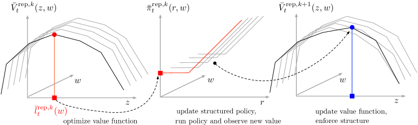
Figure 3: An illustration of the sequence of updates used in the S-AC algorithm.

Input: Lower-level optimal policy $\mu^{*}$ (learned from backward dynamic programming). Initial policy estimates $\mkern 1.5mu\overline{\mkern-0.5mul\mkern-0.5mu}\mkern 1.5mu^{\textnormal{rep},0}$ and $\bar{\pi}^{\textnormal{dis},0}$, and value estimates $\bar{v}^{\textnormal{rep},0}$ and $\bar{v}^{\textnormal{dis},0}$ (nonincreasing in $z^{\textnormal{rep}}$ and $z^{\textnormal{dis}}$ respectively). Stepsize rules $\tilde{\alpha}_{t}^{k}$ and $\tilde{\beta}_{t}^{k}$ for all $t,k$.

Output: Approximations $\mkern 1.5mu\overline{\mkern-0.5mul\mkern-0.5mu}\mkern 1.5mu^{\textnormal{rep},k}$, $\bar{\pi}^{\textnormal{dis},k}$, $\bar{v}^{\textnormal{rep},k}$, and $\bar{v}^{\textnormal{dis},k}$.

1 for $k=1,2,\ldots$ do

2       Sample initial states $z_{0}^{\textnormal{rep},k}$ and $z_{0}^{\textnormal{dis},k}$.

3       for $t=0,1,\ldots,T-1$ do

4             Observe $w_{t}^{k}$ and $\xi_{t,1}^{k}$, then observe $\hat{v}_{t}^{\textnormal{rep},k}$ and $\hat{v}_{t}^{\textnormal{dis},k}$ according to (17) and (18) respectively.

5             Perform SA step:

$$\textstyle\tilde{v}_{t}^{\textnormal{rep},k}(z^{\textnormal{rep}},w) =\bigl{(}1-\alpha_{t}^{k}(z^{\textnormal{rep}},w)\bigr{)}\,\bar{v}_{t}^{\textnormal{rep},k-1}(z^{\textnormal{rep}},w)+\alpha_{t}^{k}(z^{\textnormal{rep}},w)\,\hat{v}_{t}^{\textnormal{rep},k},$$

$$\textstyle\tilde{v}_{t}^{\textnormal{dis},k}(z^{\textnormal{dis}},w) =\bigl{(}1-\alpha_{t}^{k}(z^{\textnormal{dis}},w)\bigr{)}\,\bar{v}_{t}^{\textnormal{dis},k-1}(z^{\textnormal{dis}},w)+\alpha_{t}^{k}(z^{\textnormal{dis}},w)\,\hat{v}_{t}^{\textnormal{dis},k}.$$

6             Perform the concavity projection operation (19):

$$\textstyle\bar{v}_{t}^{\textnormal{rep},k}=\Pi_{z_{t}^{\textnormal{rep},k},w_{t}^{k}}(\tilde{v}_{t}^{\textnormal{rep},k}),\;\;\;\;\bar{v}_{t}^{\textnormal{dis},k}=\Pi_{z_{t}^{\textnormal{dis},k},w_{t}^{k}}(\tilde{v}_{t}^{\textnormal{dis},k}).$$

7             Observe and update the replenish-up-to threshold:

$$\hat{l}_{t}^{\textnormal{rep},k}=\textstyle\operatorname*{arg\,max}_{z^{\textnormal{rep}}\in\bar{\mathcal{Z}}(0)}\sum_{j=0}^{z^{\textnormal{rep}}}\bar{v}_{t}^{\textnormal{rep},k}\bigl{(}j,w_{t}^{k}\bigr{)},$$

$$\mkern 1.5mu\overline{\mkern-0.5mul\mkern-0.5mu}\mkern 1.5mu_{t}^{\textnormal{rep},k}(w)=\bigl{(}1-\beta_{t}^{k}(w)\bigr{)}\,\mkern 1.5mu\overline{\mkern-0.5mul\mkern-0.5mu}\mkern 1.5mu_{t}^{\textnormal{rep},k-1}(w)+\beta_{t}^{k}(w)\,\hat{l}_{t}^{\textnormal{rep},k}.$$

8             Observe and update the dispense-down-to policy:

9             for $z_{t}^{\textnormal{rep}}=0,1,\ldots,R_{\textnormal{max}}$  do

10                  

$$\hat{\pi}_{t}^{\textnormal{dis}}=\textstyle\operatorname*{arg\,max}_{z^{\textnormal{dis}}\in\underline{\mathcal{Z}}(z_{t}^{\textnormal{rep}})}U_{w_{t}^{k},0}^{\mu^{*}}\bigl{(}z_{t}^{\textnormal{rep}}-z^{\textnormal{dis}},\xi_{t,0}^{k}\bigr{)}+\sum_{j=0}^{z^{\textnormal{dis}}}\bar{v}_{t}^{\textnormal{dis},k}\bigl{(}j,w_{t}^{k}\bigr{)},$$

$$\bar{\pi}_{t}^{\textnormal{dis},k}(z^{\textnormal{rep}},w)=\bigl{(}1-\alpha^{k}(z^{\textnormal{rep}},w)\bigr{)}\,\bar{\pi}_{t}^{\textnormal{dis},k-1}(z^{\textnormal{rep}},w)+\alpha^{k}(z^{\textnormal{rep}},w)\,\hat{\pi}_{t}^{\textnormal{dis}}.$$

11             end for

12             If $t<T-1$, take $z_{t+1}^{\textnormal{rep},k}$ and $z_{t+1}^{\textnormal{dis},k}$ according to the $\epsilon$-greedy exploration policy.

13       end for

14      

15 end for

Algorithm 1 Structured Actor-Critic Method

• The inputs of Algorithm 1 are a random initial basestock policy $\mkern 1.5mu\overline{\mkern-0.5mul\mkern-0.5mu}\mkern 1.5mu^{\textnormal{rep},0}$, and concave, piecewise linear value function approximations $\bar{v}^{\textnormal{rep},0}$ and $\bar{v}^{\textnormal{dis},0}$.

• Each iteration $k$ consists of a loop through the time periods $t$.

• At period $t$, the approximate slopes are updated in Lines 1–1. Based on $z_{t}^{\textnormal{rep},k}$, $z_{t}^{\textnormal{dis},k}$ and $\mathbf{Z}_{t}^{k}(w_{t}^{k})$, we first observe the sequences of the predecision resource $\{r_{t+1},r_{t+2},\ldots,r_{T}\}$ and the postdecision resources $\{z_{t}^{\textnormal{rep},k},z_{t+1}^{\textnormal{rep}},\ldots,z_{T-1}^{\textnormal{rep}}\}$ and $\{z_{t}^{\textnormal{dis},k},z_{t+1}^{\textnormal{dis}},\ldots,z_{T-1}^{\textnormal{dis}}\}$. These are computed according to (2), and the equations $z_{\tau}^{\textnormal{rep}}=\tilde{\pi}_{\tau}^{\textnormal{rep},k-1}(r_{\tau},w_{\tau}^{k})$, and $z_{\tau}^{\textnormal{dis}}=\operatorname*{arg\,max}_{z^{\textnormal{dis}}\in\underline{\mathcal{Z}}(\tilde{z}_{\tau}^{\textnormal{rep}})}U_{\check{w}_{\tau}^{k},0}^{\mu^{*}}\bigl{(}\tilde{z}_{\tau}^{\textnormal{rep}}-z^{\textnormal{dis}},\check{\xi}_{\tau,0}^{k}\bigr{)}+\bar{V}_{\tau}^{\textnormal{dis},k-1}\bigl{(}z^{\textnormal{dis}},\check{w}_{\tau}^{k}\bigr{)}$ for all $\tau\geq t+1$. In the following illustration, let us take the value slope and policy corresponding to the replenish-up-to decision as an example, those corresponding to the dispense-down-to decision are similar.

• The observation of the slope $\hat{v}_{t}^{\textnormal{rep},k}$ implied by the policies $\tilde{\pi}^{\textnormal{rep},k-1}$ and $\tilde{\pi}^{\textnormal{dis},k-1}$ is computed using (15) and (17) and used to calculate the smoothed slopes $\tilde{v}_{t}^{\textnormal{rep},k}(z^{\textnormal{rep}},w)$ in Line 1, where $\alpha_{t}^{k}(z^{\textnormal{rep}},w)=\tilde{\alpha}_{t}^{k}\mathbbm{1}\{z^{\textnormal{rep}}=z_{t}^{\textnormal{rep},k}\}\mathbbm{1}\{w=w_{t}^{k}\}$. Thus, only the state $(z_{t}^{\textnormal{rep},k},w_{t}^{k})$ is updated.

• A concavity projection operation in Line 1 is performed on the slopes $\tilde{v}_{t}^{\textnormal{rep},k}$, resulting in a new set of slopes $\Pi_{z_{t}^{\textnormal{rep},k},w_{t}^{k}}(\tilde{v}_{t}^{\textnormal{rep},k})$, in order to avoid violation of concavity. The component of $\Pi_{z_{t}^{\textnormal{rep},k},w_{t}^{k}}(\tilde{v}_{t}^{\textnormal{rep},k})$ at state $(z^{\textnormal{rep}},w)$ is

  $$\Pi_{z_{t}^{\textnormal{rep},k},w_{t}^{k}}(\tilde{v}_{t}^{\textnormal{rep},k})[z^{\textnormal{rep}},w]$$ (19)

  $$=\begin{cases}\tilde{v}_{t}^{\textnormal{rep},k}(z_{t}^{\textnormal{rep},k},w_{t}^{k})&\text{if}\;\;w=w_{t}^{k},\;z^{\textnormal{rep}}<z_{t}^{\textnormal{rep},k},\;\tilde{v}_{t}^{\textnormal{rep},k}(z^{\textnormal{rep}},w)<\tilde{v}_{t}^{\textnormal{rep},k}(z_{t}^{\textnormal{rep},k},w_{t}^{k})\\ &\text{or}\;w=w_{t}^{k},\;z^{\textnormal{rep}}>z_{t}^{\textnormal{rep},k},\;\tilde{v}_{t}^{\textnormal{rep},k}(z^{\textnormal{rep}},w)>\tilde{v}_{t}^{\textnormal{rep},k}(z_{t}^{\textnormal{rep},k},w_{t}^{k}),\\ \tilde{v}_{t}^{\textnormal{rep},k}(z^{\textnormal{rep}},w)&\text{otherwise}.\end{cases}$$

• The approximate replenish-up-to policy is updated in Lines 1. The observation $\hat{l}_{t}^{\textnormal{rep},k}$ is the maximum point of $\bar{V}_{t}^{\textnormal{rep},k}(\cdot,w_{t}^{k})$ inside the set $\mathcal{Z}(0)$, which is the implied replenish-up-to basestock threshold from the value function approximation. Given the observation, the policy is updated with stepsize $\beta_{t}^{k}(w)=\tilde{\beta}_{t}^{k}\mathbbm{1}\{w=w_{t}^{k}\}$.

• The approximate dispense-down-to policy is updated in Lines 1–1. For each $z^{\textnormal{rep}}$, we can observe $\hat{\pi}_{t}^{\textnormal{dis}}$ according to (9). The policy is updated with the observation and stepsize $\alpha_{t}^{k}(z^{\textnormal{rep}},w)=\tilde{\alpha}_{t}^{k}\mathbbm{1}\{z^{\textnormal{rep}}=z_{t}^{\textnormal{rep}}\}\mathbbm{1}\{w=w_{t}^{k}\}$.

• Finally, the next replenish-up-to decision follows an $\epsilon$-greedy policy, which is to select $z_{t+1}^{\textnormal{rep},k}=\tilde{\pi}_{\tau}^{\textnormal{rep},k-1}(r_{\tau},w_{\tau}^{k})$ with probability $1-\epsilon$, or take $z_{t+1}^{\textnormal{rep},k}$ randomly from $\mathcal{Z}(r_{t+1}^{k})$ with probability $\epsilon$. In our numerical experiments, $\epsilon$ is chosen to be 0.1.

Figure 3 illustrates how the replenish-up-to value function and policy approximations interact with each other. The first two panels together show that given a structured value function, its maximizer (red square) is used to update the structured policy. Panels two and three together show that an observation of the current policy’s value (blue circle) is in turn used to update the structured value function (where a projection step occurs to enforce structure). The process then repeats with the new maximizer (blue square).

Convergence Analysis

In this section, we give some theoretical assumptions and then state the convergence of Algorithm 1; in particular, the convergence of both the value function approximations $\bar{v}^{\textnormal{rep},k}$ and $\bar{v}^{\textnormal{dis},k}$ and the basestock policies $\mkern 1.5mu\overline{\mkern-0.5mul\mkern-0.5mu}\mkern 1.5mu^{\textnormal{rep},k}$ and $\bar{\pi}^{\textnormal{dis},k}$. Let $\{\bar{v}_{t}^{\textnormal{rep},k}\}_{k\geq 0}$ and $\{\bar{v}_{t}^{\textnormal{dis},k}\}_{k\geq 0}$ be the sequences of slopes, let $\{\mkern 1.5mu\overline{\mkern-0.5mul\mkern-0.5mu}\mkern 1.5mu_{t}^{\textnormal{rep},k}\}_{k\geq 0}$ and $\{\bar{\pi}_{t}^{\textnormal{dis},k}\}_{k\geq 0}$, be the sequences of policies generated by the algorithm. For period $T$, we assume $v_{T}^{\textnormal{rep}}(z^{\textnormal{rep}},w)=0$ for all iterations $k\geq 0$ and all possible postdecision states $(z^{\textnormal{rep}},w)$, as we only need to learn the policy and slopes up to period $T-1$. We work on a probability space $(\Omega,\mathcal{F},\mathbf{P})$, where $\mathcal{F}=\sigma\{(r_{t}^{k},z_{t}^{\textnormal{rep},k},z_{t}^{\textnormal{dis},k},w_{t}^{k},\bm{\xi}_{t}^{k},\mathbf{D}_{t}^{k},\hat{v}_{t}^{k}),\,t\leq T,\,k\geq 0\}$, where $\bm{\xi}_{t}^{k}=(\xi_{t,1}^{k},\xi_{t,2}^{k},\ldots,\xi_{t,n_{k}}^{k})$, $\mathbf{D}_{t}^{k}=(D_{t,1}^{k},D_{t,2}^{k},\ldots,D_{t,n_{k}}^{k})$. Moreover, we define

$$\mathcal{F}_{t}^{k}=\sigma\bigl{\{}\{(r_{\tau}^{k^{\prime}},z_{\tau}^{\textnormal{rep},k^{\prime}},z_{\tau}^{\textnormal{dis},k^{\prime}},w_{\tau}^{k^{\prime}},\bm{\xi}_{\tau}^{k^{\prime}},\mathbf{D}_{\tau}^{k^{\prime}},\hat{v}_{\tau}^{k^{\prime}}),{k^{\prime}}<k,\tau\leq T\}\cup\{(r_{\tau}^{k},z_{\tau}^{\textnormal{rep},k},z_{\tau}^{\textnormal{dis},k},w_{\tau}^{k},\bm{\xi}_{\tau}^{k},\mathbf{D}_{\tau}^{k},\hat{v}_{t}^{k}),\tau\leq t\}\bigr{\}},$$

for $t\leq T-1$ and $k\geq 1$, with $\mathcal{F}_{t}^{0}=\{\emptyset,\Omega\}$ for all $t\leq T$. Their relationships are $\mathcal{F}_{t}^{k}\subseteq\mathcal{F}_{t+1}^{k}$ for $t\leq T-1$ and $\mathcal{F}_{T}^{k}\subseteq\mathcal{F}_{0}^{k+1}$.

Assumption 2.

For any $z$ and $w$, suppose the stepsize sequences $\bigl{\{}\alpha_{t}^{k}(z^{\textnormal{rep}},w)\bigr{\}}$, $\bigl{\{}\alpha_{t}^{k}(z^{\textnormal{dis}},w)\bigr{\}}$, and $\{\beta_{t}^{k}(w)\}$ satisfy the following conditions:

1. For $\textnormal{x}\in\{\textnormal{rep},\textnormal{dis}\}$, $\alpha_{t}^{k}(z^{\textnormal{x}},w)=\tilde{\alpha}_{t}^{k}\mathbbm{1}\{z^{\textnormal{x}}=z_{t}^{\textnormal{x},k}\}\mathbbm{1}\{w=w_{t}^{k}\}$ for some $\tilde{\alpha}_{t}^{k}\in\mathbb{R}$ that is $\mathcal{F}_{t}^{k}$-measurable,

2. $\beta_{t}^{k}(w)=\tilde{\beta}_{t}^{k}\mathbbm{1}\{w=w_{t}^{k}\}$ for some $\tilde{\beta}_{t}^{k}\in\mathbb{R}$ that is $\mathcal{F}_{t}^{k}$-measurable,

3. For $\textnormal{x}\in\{\textnormal{rep},\textnormal{dis}\}$, $\sum_{k=0}^{\infty}\alpha_{t}^{k}(z^{\textnormal{x}},w)=\infty$, $\sum_{k=0}^{\infty}\,\bigl{(}\alpha_{t}^{k}(z^{\textnormal{x}},w)\bigr{)}^{2}<\infty$ almost surely,

4. $\sum_{k=0}^{\infty}\beta_{t}^{k}(w)=\infty$, $\sum_{k=0}^{\infty}\,\bigl{(}\beta_{t}^{k}(w)\bigr{)}^{2}<\infty$ almost surely.

Assumption 2(1) and (2) ensures that only the slope and threshold for the observed state is updated in Line 1 of Algorithm 1; the ones corresponding to unobserved states are kept the same until the projection step. Parts (3) and (4) are standard conditions on the stepsize. To keep the convergence results clean, we also assume the state-dependent basestock thresholds are unique (this assumption can be easily relaxed).

Assumption 3.

There is a unique optimal solution to $\max_{z\in\mathcal{Z}(0)}\;\tilde{V}_{t}^{\textnormal{rep}}(z,w)$, which implies that there is a single optimal replenishment basestock threshold for each $w$. The unique optimal solution assumption also applies to $\tilde{V}_{t}^{\textnormal{dis}}$.

Assumptions (1)-(3) are used for the next two results. The primary novel aspect of our analysis is to connect the approximate policies with the approximate value functions through the structural properties of the problem. Before stating the main convergence result, Theorem 1, we introduce a lemma that illustrates the crucial mechanism for convergence.

Lemma 1.

The following hold:

1. For any fixed period $t$, suppose that the policies $\bar{\pi}_{\tau}^{\textnormal{rep},k}\rightarrow\pi_{\tau}^{\textnormal{rep}}$ almost surely for $\tau\geq t+1$, and $\bar{\pi}_{\tau}^{\textnormal{dis},k}\rightarrow\pi_{\tau}^{\textnormal{dis}}$ almost surely for $\tau\geq t$. Then it holds that $\bar{v}_{t}^{\textnormal{rep},k}(z^{\textnormal{rep}},w)\rightarrow v_{t}^{\textnormal{rep}}(z^{\textnormal{rep}},w)$ almost surely.

2. For any fixed period $t$, suppose that the policies $\bar{\pi}_{\tau}^{\textnormal{rep},k}\rightarrow\pi_{\tau}^{\textnormal{rep}}$ and $\bar{\pi}_{\tau}^{\textnormal{dis},k}\rightarrow\pi_{\tau}^{\textnormal{dis}}$ almost surely for $\tau\geq t+1$. Then it holds that $\bar{v}_{t}^{\textnormal{dis},k}(z^{\textnormal{dis}},w)\rightarrow v_{t}^{\textnormal{dis}}(z^{\textnormal{dis}},w)$ almost surely.

Sketch of Proof.

Let us show part (1) of the lemma. The proof for part (2) is similar. We first construct two deterministic sequences $\{G^{m}\}$ and $\{I^{m}\}$ such that $G^{0}=v^{\textnormal{rep}}+v_{\text{max}}^{\textnormal{rep}}$ and $I^{0}=v^{\textnormal{rep}}-v_{\text{max}}^{\textnormal{rep}}$ with

$$G^{m+1}=\frac{G^{m}+v^{\textnormal{rep}}}{2}\quad\text{and}\quad I^{m+1}=\frac{I^{m}+v^{\textnormal{rep}}}{2},$$

where $|v_{t}^{\textnormal{rep}}(z^{\textnormal{rep}},w)|\leq v_{\text{max}}^{\textnormal{rep}}$ for all $t$, $z^{\textnormal{rep}}$, and $w$. These sequences have been previously used in Bertsekas and Tsitsiklis (1996). Lemma 1 is proved if we have

$$I_{t}^{m}(z^{\textnormal{rep}},w)\leq\bar{v}_{t}^{\textnormal{rep},k-1}(z^{\textnormal{rep}},w)\leq G_{t}^{m}(z^{\textnormal{rep}},w),$$ (20)

for any $m$ and sufficiently large $k$. The proof proceeds by showing the following.

1. Define noise terms $\epsilon_{t}^{k}(z_{t}^{\textnormal{rep},k},w_{t}^{k})=\mathbf{E}\bigl{[}\hat{v}_{t}^{\textnormal{rep},k}\bigr{]}-v_{t}^{\textnormal{rep}}(z_{t}^{\textnormal{rep},k},w_{t}^{k})$ and $\varepsilon_{t}^{k}(z_{t}^{\textnormal{rep},k},w_{t}^{k})=\hat{v}_{t}^{\textnormal{rep},k}-\mathbf{E}\bigl{[}\hat{v}_{t}^{\textnormal{rep},k}\bigr{]}$. Recall that $\hat{v}_{t}^{\textnormal{rep},k}=\hat{V}_{t}^{\textnormal{rep},k}(z_{t}^{\textnormal{rep},k},w_{t}^{k})-\hat{V}_{t}^{\textnormal{rep},k}(z_{t}^{\textnormal{rep},k}-1,w_{t}^{k})$, where

   $$\hat{V}_{t}^{\textnormal{rep},k}(z^{\textnormal{rep}},w_{t}^{k})= -c_{w_{t}^{k}}z^{\textnormal{rep}}+U_{\check{w}_{t}^{k},0}^{\mu^{*}}\bigl{(}z^{\textnormal{rep}}-\tilde{\pi}_{t}^{\textnormal{dis},k-1}(z^{\textnormal{rep}},w_{t}^{k}),\check{\xi}_{t,0}^{k}\bigr{)}$$

   $$+f_{t}^{\textnormal{dis}}\bigl{(}\tilde{\pi}^{\textnormal{rep},k-1},\tilde{\pi}^{\textnormal{dis},k-1};\mathbf{Z}^{k}_{t}(w_{t}),z^{\textnormal{rep}}\bigr{)}.$$

   From the assumption that $\bar{\pi}_{\tau}^{\textnormal{rep},k}\rightarrow\pi_{\tau}^{\textnormal{rep}}$ and $\bar{\pi}_{\tau}^{\textnormal{dis},k}\rightarrow\pi_{\tau}^{\textnormal{dis}}$ almost surely for all $\tau\geq t+1$, and the fact that $f_{t}^{\textnormal{dis}}\bigl{(}\tilde{\pi}^{\textnormal{rep},k-1},\tilde{\pi}^{\textnormal{dis},k-1};\mathbf{Z}^{k}_{t}(w),z^{\textnormal{rep}}\bigr{)}$ depends on the replenish-up-to policies for periods $t+1$ onward and the dispense-down-to policies for periods $t$ onward, we conclude that

   $$\mathbf{E}_{w}\bigl{[}f_{t}^{\textnormal{dis}}\bigl{(}\tilde{\pi}^{\textnormal{rep},k-1},\tilde{\pi}^{\textnormal{dis},k-1};\mathbf{Z}_{t}^{k}(w),z^{\textnormal{rep}}\bigr{)}\bigr{]}\rightarrow\tilde{V}_{t}^{\textnormal{dis}}\bigl{(}\pi_{t}^{\textnormal{dis},*}(z^{\textnormal{rep}},w),w\bigr{)}$$

   almost surely. Therefore, $\epsilon_{t}^{k}(z_{t}^{\textnormal{rep},k},w_{t}^{k})$ converges to zero almost surely and $\varepsilon_{t}^{k}(z_{t}^{\textnormal{rep},k},w_{t}^{k})$ is unbiased.

2. We partition the state space $\mathcal{S}$ into two parts: (1) states $(z^{\textnormal{rep}},w)\in\mathcal{S}^{-}_{t}$ and (2) states $(z^{\textnormal{rep}},w)\in\mathcal{S}\setminus\mathcal{S}_{t}^{-}$, where $\mathcal{S}_{t}^{-}$ is a random set of states that are increased by the projection operator (19) on finitely many iterations $k$. The proof considers each partition separately to show (20). For states $(z^{\textnormal{rep}},w)\in\mathcal{S}^{-}_{t}$, we show by forward induction on $m$ the existence of a finite index $\tilde{K}_{t}^{m}$ such that (20) holds for all iterations $k\geq\tilde{K}_{t}^{m}$. The proof utilizes stochastic sequences related to the noise terms and stochastic “bounding” sequences. For any state $(z^{\textnormal{rep}},w)\in\mathcal{S}\setminus\mathcal{S}^{-}_{t}$ and a fixed $m$, by Lemma 6.4 of Nascimento and Powell (2009), we show the existence of a state-dependent random index $\hat{K}_{t}^{m}(z^{\textnormal{rep}},w)$ such that (20) holds for all $k\geq\hat{K}_{t}^{m}(z^{\textnormal{rep}},w)$.

See Appendix A.3 for the full details of the proof. ∎

Lemma 1 implies the convergence of the approximate slopes $\bar{v}^{k}$ to the true slopes $v$ as long as the policy approximation converges correctly.

Theorem 1.

For $\textnormal{x}\in\{\textnormal{rep},\textnormal{dis}\}$, the slope approximation $\bar{v}_{t}^{\textnormal{x},k}(z^{\textnormal{x}},w)$ converges to the slope of the postdecision value function $v_{t}^{\textnormal{x}}(z^{\textnormal{x}},w)$ almost surely for all $(z^{\textnormal{x}},w)$ and $t$; the policy approximations $\bar{\pi}_{t}^{\textnormal{rep},k}(r,w)$ and $\bar{\pi}_{t}^{\textnormal{dis},k}(z^{\textnormal{rep}},w)$ respectively converge to the optimal policies $\pi_{t}^{\textnormal{rep}}(r,w)$ and $\pi_{t}^{\textnormal{dis}}(z^{\textnormal{rep}},w)$ almost surely for all $r$, $z^{\textnormal{rep}}$, $w$ and $t$.

Sketch of Proof.

The proof depends inductively on Lemma 1. Given its result for period $t$, we can then argue the convergence of policy approximations $\bar{\pi}_{t}^{\textnormal{rep},k}(r,w)$ and $\bar{\pi}_{t}^{\textnormal{dis},k}(z^{\textnormal{rep}},w)$. This allows us to re-apply Lemma 1 on period $t-1$. The details are given in Appendix A.4. ∎

Numerical Experiments

In this section, we test the performance of our algorithm empirically and compare its convergence rate with other ADP algorithms on a common set of several benchmark problems with different state space sizes. Specifically, we compare with SPAR, a standard actor-critic method with a linear architecture, a policy gradient method with a linear architecture, and tabular Q-learning. We begin by giving a brief description of these algorithms.

• The multi-stage version of SPAR, introduced in Nascimento and Powell (2009), takes advantage of the concavity of the value function and uses the temporal difference to update slopes without a policy approximation. More specifically, in order to generate observations $\hat{V}_{t}^{\textnormal{rep},k}$ and $\hat{V}_{t}^{\textnormal{dis},k}$, instead of using (15) and (16), SPAR uses

  $$\textstyle\hat{V}_{t}^{\textnormal{rep},k}(z^{\textnormal{rep}},w_{t}^{k})=-c_{w_{t}^{k}}z^{\textnormal{rep}}+\max_{z^{\textnormal{dis}}\leq z^{\textnormal{rep}}}\bigl{\{}U_{w_{t}^{k},0}^{\mu^{*}}\bigl{(}z^{\textnormal{rep}}-z^{\textnormal{dis}},\xi_{t,0}^{k}\bigr{)}+\bar{V}_{t}^{\textnormal{dis},k-1}\bigl{(}z^{\textnormal{dis}},w_{t}^{k}\bigr{)}\bigr{\}},$$

  and

  $$\textstyle\hat{V}_{t}^{\textnormal{dis},k}(z^{\textnormal{dis}},w_{t}^{k})=(c_{w_{t+1}}-h)z^{\textnormal{dis}}+\max_{z^{\textnormal{rep}}\geq z^{\textnormal{dis}}}\bar{V}_{t+1}^{\textnormal{rep},k-1}\bigl{(}z^{\textnormal{rep}},w_{t+1}\bigr{)}$$

  respectively. Although the original specification of SPAR does not use an exploration policy, we implemented $\epsilon$-greedy with exploration rate $0.1$ for improved performance.

• We implement an actor-critic (AC) method (Sutton and Barto, 1998) based on a linear approximation architecture for both the policy and value approximations. In both cases, the basis functions are chosen to be Gaussian radial basis functions (RBFs). The “critic” approximates the value function using a weighted sum of RBF basis functions. The “actor” is a stochastic policy with a parameter $h_{t}(r,w;z^{\textnormal{rep}},z^{\textnormal{dis}})$ for each state-action pair $(r,w;z^{\textnormal{rep}},z^{\textnormal{dis}})$, and is also approximated using a weighted sum of RBFs, which indicate the tendency of selecting action $(z^{\textnormal{rep}},z^{\textnormal{dis}})$ in state $(r,w)$. The associated stochastic policy is obtained through a softmax function, so that the probability of taking action $(z^{\textnormal{rep}},z^{\textnormal{dis}})$ in state $(r,w)$ is $\pi_{t}(z^{\textnormal{rep}},z^{\textnormal{dis}}\,|\,r,w)=e^{h(r,w;z^{\textnormal{rep}},z^{\textnormal{dis}})}/\sum_{(z_{1},z_{2})}e^{h(r,w;z_{1},z_{2})}.$ Detailed steps of the method are shown in Appendix B.

• Our policy gradient (PG) method (Williams, 1992; Sutton et al., 2000) updates the stochastic policy in each iteration. We adopt the Monte-Carlo policy gradient method where the policy approximation follows the same softmax policy as in the AC algorithm above. There is no value function and the policy parameters are updated using a sampled cumulative reward from $t$ to $T$.

• The previous two algorithms use linear architectures for generalization. We also compare to the widely-used Q-learning (QL) algorithm (Watkins, 1989), which is called tabular because each state-action pair is updated independently (structured actor-critic and SPAR lie in-between these two extremes as they generalize by enforcing structure). Q-learning aims to learn the state-action value function:

  $$Q_{t}(r,w;z^{\textnormal{rep}},z^{\textnormal{dis}})=(c_{w}-h)r-c_{w}z^{\textnormal{rep}}+\mathbf{E}_{w}\bigl{[}U_{w_{t},0}^{\mu^{*}}(z^{\textnormal{rep}}-z^{\textnormal{dis}},\Xi_{t,0})+V_{t+1}\left(z^{\textnormal{dis}},W_{t+1}\right)\bigr{]}.$$

  Our implementation is a standard finite-horizon version of the algorithm that uses an $\epsilon$-greedy exploration policy at a rate of $0.1$.

Optimal benchmarks used to determine the effectiveness of the five algorithms were computed using standard backward dynamic programming (BDP). All computations in this paper were performed using Python 3.5.

Benchmark Instances and Parameters

We consider 10 PODs in these synthetic benchmark instances. Each POD has a randomly generated attribute ranging between 0 and 1 representing its priority, which is reflected in the utility function $u$. Let the stochastic utility function be $\tilde{u}\bigl{(}\min(y_{i},D_{i}),\xi_{i}\bigr{)}$, with expectation $u_{w}(x_{i},\xi_{i})=\mathbf{E}_{w}\bigl{[}\tilde{u}\bigl{(}\min(\mu_{i}(x_{i},\xi_{i}),D_{i}),\xi_{i}\bigr{)}\bigr{]}$, where $\mu_{i}$ and $D_{i}$ are respectively the policy and the amount of demand in sub-period $i$. Let $\tilde{u}\bigl{(}z,\xi_{i}\bigr{)}$ be nondecreasing and discretely concave in $z$, then $\tilde{u}\bigl{(}\min(y_{i},D_{i}),\xi_{i}\bigr{)}$ is $L^{\natural}$-concave in $y_{i}$ based on Lemma 2 in Chen et al. (2014), the structural properties are kept for this stochastic utility function. For each exogenous information realization $w$, we randomly generated 10 different patterns of the arriving POD sequences.

Our interpretation of the stochastic process $\{W_{t}\}$ is a signal of the total demand for period $t$. For benchmarking purposes, we use the model $W_{t+1}=\varphi_{t}W_{t}+\hat{W}_{t+1}$, where $\varphi_{t}$ is deterministic and $\hat{W}_{t+1}$ is an independent noise term that follows a mean zero discretized normal distribution with standard deviation $\sigma_{t+1}$. In this paper, a continuously distributed random variable $X$ is discretized to $X_{\textnormal{disc}}$ with $\mathbf{P}(X_{\textnormal{disc}}=x)=\mathbf{P}(X\leq x)-\mathbf{P}(X\leq x-1)$. Given a demand signal $W_{t}=w_{t}$, the realized demand $D_{t,i}$ is a discretized normal distribution with mean $d_{i}(w_{t})$ and standard deviation $\tilde{\sigma}_{t}=3$ for $i=1,2,\ldots,n$. All of the means above were generated randomly.

We created 25 benchmark problem instances by varying the sizes of the state, action, and outcome spaces (i.e., number of possible values of the exogenous information). Specifically, we consider problem instances with 21, 31, 41, 51, and 61 inventory levels and 3, 6, 9, 12, and 15 information states; these are the columns and rows shown in Tables 1 and 2. The sizes of the action spaces corresponding to inventory level sizes 21, 31, 41, 51, and 61 are respectively 231, 496, 861, 1326, and 1891. The time horizon for each instance is $T=10$ and the cost parameters are $b=0$, $h=5$, $c_{w}\in[10,50]$, $\mathbf{E}[c_{w}]=30$.

Table 1: Performance (% optimality) at iterations 500 and 1000.

		At iteration 500					At iteration 1000
$R_{\textnormal{max}}$	$|\mathcal{W}|$	3	6	9	12	15	3	6	9	12	15
20	AC	97.20	97.68	98.01	97.41	96.88	98.86	99.03	98.50	98.38	97.60
	PG	73.04	76.02	72.35	76.64	74.29	77.94	79.12	73.35	79.16	75.38
	QL	30.02	33.86	28.36	27.85	35.53	32.60	35.91	31.75	31.20	37.63
	S-AC (ours)	99.76	99.26	98.33	97.68	97.45	99.83	99.57	99.00	98.48	98.50
	SPAR	97.82	95.11	95.10	94.69	92.36	96.95	97.55	93.80	94.33	95.87
30	AC	97.21	96.40	95.75	95.17	94.91	97.65	97.13	96.40	96.31	95.27
	PG	69.97	72.24	76.48	73.36	78.19	76.07	74.15	76.91	81.04	78.30
	QL	38.26	34.09	28.84	27.47	34.21	40.35	37.14	35.43	33.99	37.78
	S-AC (ours)	99.58	99.36	98.53	97.70	97.61	99.83	99.67	99.18	98.67	98.60
	SPAR	97.85	97.94	92.57	95.11	92.58	98.62	97.88	95.24	95.12	94.46
40	AC	96.30	95.16	91.63	93.24	92.15	96.70	96.05	92.56	93.94	92.54
	PG	72.95	77.04	75.57	73.92	78.39	76.51	77.78	75.90	75.39	79.15
	QL	39.65	35.40	26.71	24.70	32.36	42.20	40.57	35.20	33.44	37.63
	S-AC (ours)	99.45	99.35	97.95	97.86	97.50	99.65	99.61	98.90	98.53	98.43
	SPAR	97.46	96.08	93.50	93.79	93.74	96.79	96.62	95.33	93.81	92.07
50	AC	90.96	90.56	86.47	88.00	88.02	91.65	91.76	87.18	89.03	89.73
	PG	72.06	70.67	66.57	69.34	76.81	73.95	74.75	67.71	71.71	78.05
	QL	41.63	36.35	26.26	22.00	29.87	47.68	42.72	35.22	31.90	35.60
	S-AC (ours)	99.42	99.15	97.49	97.47	97.09	99.52	99.46	98.18	98.25	98.01
	SPAR	95.54	96.65	90.91	91.27	94.02	97.39	96.30	92.21	94.35	90.38
60	AC	91.30	91.16	86.67	87.21	88.23	92.27	92.32	88.32	87.85	90.17
	PG	74.15	71.73	61.39	63.98	68.90	76.80	71.55	65.77	66.25	70.86
	QL	42.03	33.88	22.51	19.95	27.38	47.13	41.37	33.10	31.44	33.40
	S-AC (ours)	99.16	99.00	96.50	97.08	96.70	99.25	99.20	96.81	97.52	97.00
	SPAR	96.40	95.55	91.52	93.63	90.73	95.89	95.51	94.18	92.64	91.51

Table 2: Performance (% optimality) after 5 and 10 seconds of CPU time.

		CPU time = 5s					CPU time = 10s
$R_{\textnormal{max}}$	$|\mathcal{W}|$	3	6	9	12	15	3	6	9	12	15
20	AC	91.97	93.91	92.29	93.21	89.98	94.80	95.93	94.87	95.32	94.32
	PG	65.49	68.53	66.84	68.06	71.71	67.85	72.33	71.14	71.83	73.27
	QL	32.60	35.91	31.75	31.20	37.63	32.60	35.91	31.75	31.20	37.63
	S-AC (ours)	99.79	99.52	98.71	98.20	98.03	99.83	99.57	99.00	98.48	98.50
	SPAR	97.84	96.93	94.19	92.20	92.83	96.95	97.55	93.80	94.33	95.87
30	AC	89.78	89.61	88.64	88.31	88.74	93.20	91.90	92.62	91.26	91.77
	PG	68.84	64.37	71.91	67.15	74.40	67.55	68.01	73.35	65.14	74.44
	QL	40.35	37.14	35.43	33.99	37.78	40.35	37.14	35.43	33.99	37.78
	S-AC (ours)	99.62	99.39	98.00	97.37	97.40	99.80	99.67	99.01	98.35	98.35
	SPAR	95.97	97.42	94.97	94.85	94.96	97.53	97.88	92.86	94.90	95.37
40	AC	86.28	89.01	83.92	86.91	85.08	92.58	92.27	89.01	89.08	88.65
	PG	68.08	63.96	72.25	61.87	73.68	69.73	68.89	71.53	67.61	73.01
	QL	42.20	40.57	35.20	33.44	37.63	42.20	40.57	35.20	33.44	37.63
	S-AC (ours)	99.43	98.94	96.85	96.58	95.63	99.58	99.41	98.32	97.94	97.57
	SPAR	97.73	96.98	92.88	92.47	92.49	96.60	96.28	95.10	92.54	92.97
50	AC	86.79	81.48	79.76	81.90	80.34	88.10	88.05	82.45	84.92	83.29
	PG	67.47	68.04	63.74	60.86	69.41	66.57	65.26	65.34	65.01	71.29
	QL	47.60	42.72	35.22	31.34	35.60	47.68	42.72	35.22	31.90	35.60
	S-AC (ours)	98.92	98.51	95.10	94.60	93.92	99.36	99.06	97.01	96.83	96.33
	SPAR	96.85	96.62	93.17	88.63	91.35	95.02	96.27	94.17	92.61	92.27
60	AC	77.05	76.73	73.10	74.15	76.31	78.78	80.14	76.33	76.38	78.48
	PG	66.10	58.84	56.40	59.41	64.81	69.42	59.67	57.36	60.11	65.73
	QL	44.75	38.60	26.78	26.41	31.62	47.13	41.37	33.10	31.44	33.40
	S-AC (ours)	98.65	98.02	93.17	93.20	92.31	99.05	98.75	95.41	96.16	95.11
	SPAR	95.45	95.26	90.50	92.43	92.41	95.90	96.15	93.45	93.11	93.02

Optimality Gap of Approximate Policies

To estimate the value $V^{\tilde{\pi}^{k}}_{0}$ of an approximate policy $\tilde{\pi}^{k}$, we averaged the value of initial states $(r,w)$ drawn from a uniform distribution, where the value $V^{\tilde{\pi}^{k}}_{0}(r,w)$ is obtained from 100 Monte Carlo simulations following policy $\tilde{\pi}^{k}$. To evaluate the approximate policy learned from an ADP algorithm, we run 10 independent replications of the algorithm and average the performance of the learned approximate policy in each replication. Denote $\bar{V}^{\tilde{\pi}^{k}}_{0}$ the evaluation of the approximate policy learned from an algorithm. The percentage of optimality is the ratio of $\bar{V}^{\tilde{\pi}^{k}}_{0}$ to $V_{0}$, where the optimal value function $V_{0}$ is computed using BDP.

Tables 1 and 2 show the percentage of optimality of each algorithm at specific iterations and CPU times, across all problem instances. In almost all instances and comparison points, S-AC outperforms the baseline algorithms. AC is the most competitive baseline with respect to the number of iterations and SPAR is the most competitive when CPU time is of primary interest. Within the same number of iterations and CPU times, the performance of all the ADP algorithms becomes worse as the size of the problem increases; however, S-AC seems to be less sensitive than the others to problem size. Let us compare the percentage of optimality of the instance with $R_{\textnormal{max}}=20$ and $|\mathcal{W}|=3$ and the instance with $R_{\textnormal{max}}=60$ and $|\mathcal{W}|=15$ at iteration 1,000. The performance of AC, S-AC, and SPAR on the latter large instance is respectively 7.2, 2.8, and 6.5 percentage worse than the performance on the smaller instance. For the same instance at CPU time 10 seconds, the performance of the three algorithms on the larger instance is respectively 14.7, 4.7, and 4.9 percentage points worse than the performance on the smaller instance.

To further illustrate the performance of each ADP algorithm, we show the convergence curves of three instances with different sizes. Let us consider three problem instances: (1) $R_{\textnormal{max}}=20$, $|\mathcal{W}|=3$, (2) $R_{\textnormal{max}}=40$, $|\mathcal{W}|=9$, and (3) $R_{\textnormal{max}}=60$, $|\mathcal{W}|=15$. Figure 4 shows the rate of convergence of the ADP algorithms considered in this paper as a function of the number of iterations, while Figure 5 shows the rate of convergence as a function of the computation time. We plot “log regret” (log of the suboptimality from 100%) to help improve the visualization.

The policy approximations used in AC and PG are parameterized as stochastic policies initialized to take uniformly random actions in each state. This exploration helps to generate relatively high value in early iterations. AC and PG are very competitive with our S-AC algorithm when comparing performance with respect to the iteration count. However, this comes at a computational cost: although stochasticity encourages exploration, Figure 5 shows that each iteration is particularly time-consuming when compared to deterministic policies.

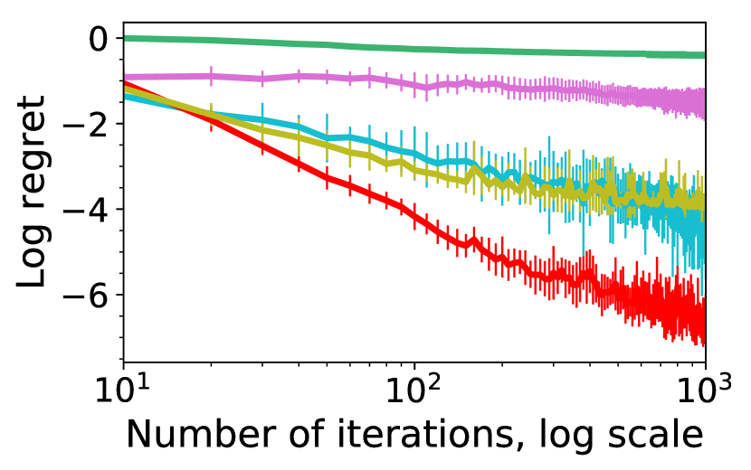
(a) $R_{\textnormal{max}}=20,|\mathcal{W}|=3$

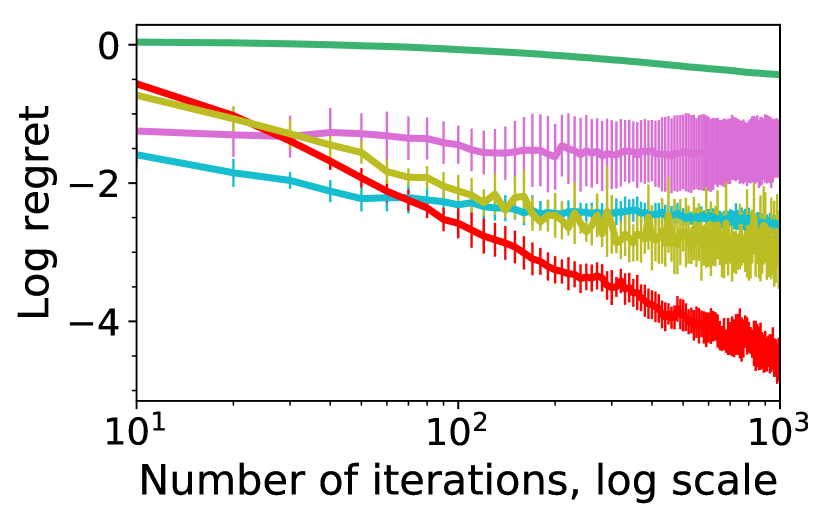
(b) $R_{\textnormal{max}}=40,|\mathcal{W}|=9$

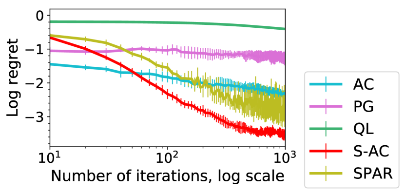
(c) $R_{\textnormal{max}}=60,|\mathcal{W}|=15$

Figure 4: Comparison of ADP algorithms with respect to iteration number.

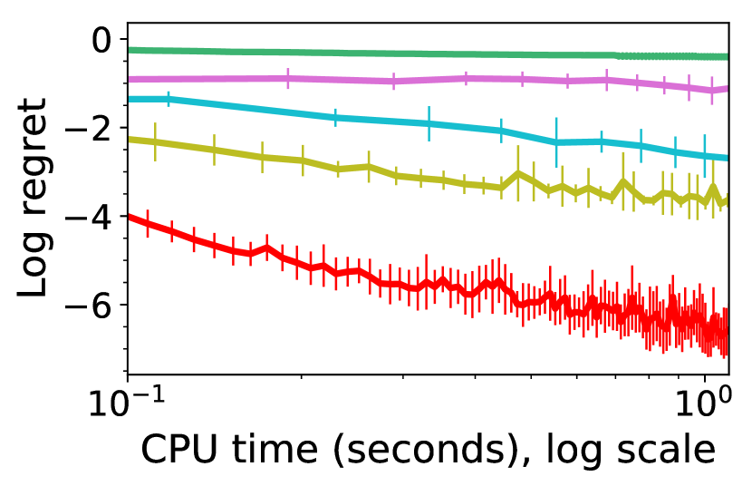
(a) $R_{\textnormal{max}}=20,|\mathcal{W}|=3$

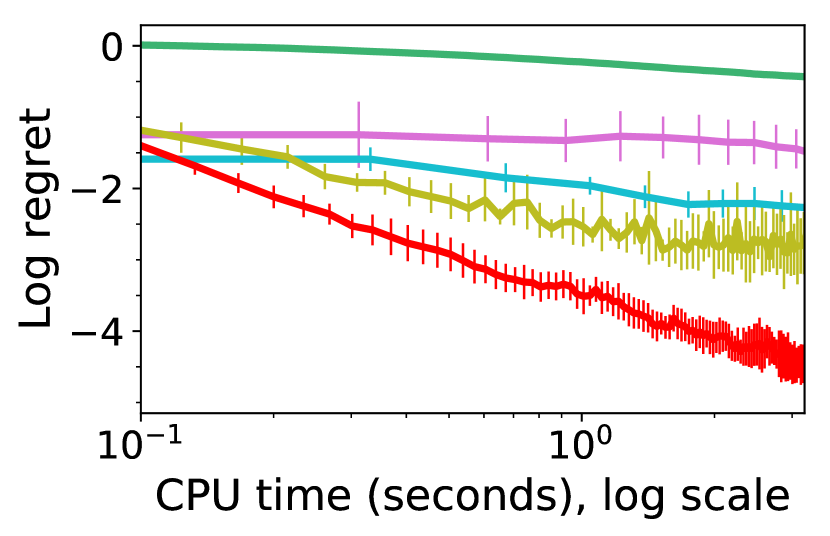
(b) $R_{\textnormal{max}}=40,|\mathcal{W}|=9$

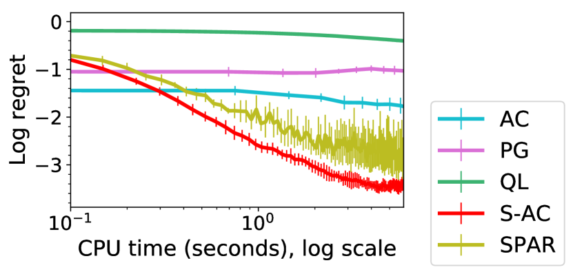
(c) $R_{\textnormal{max}}=60,|\mathcal{W}|=15$

Figure 5: Comparison of ADP algorithms with respect to CPU time.

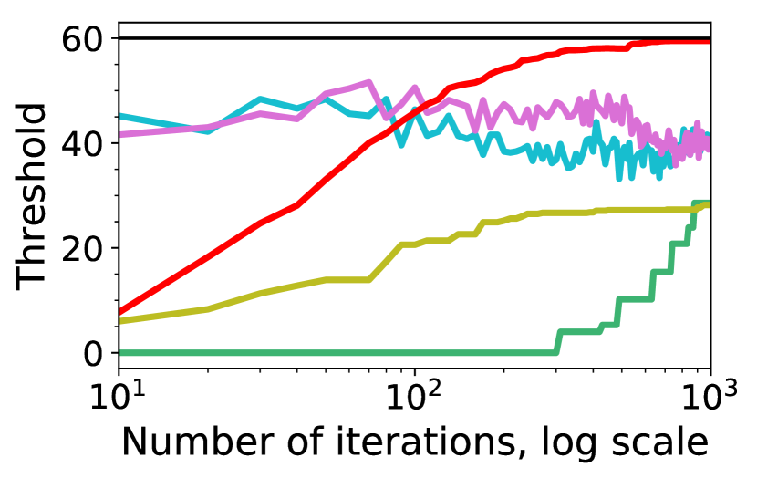
(a) $w_{0}=1$

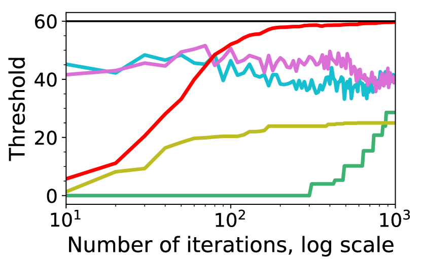
(b) $w_{0}=4$

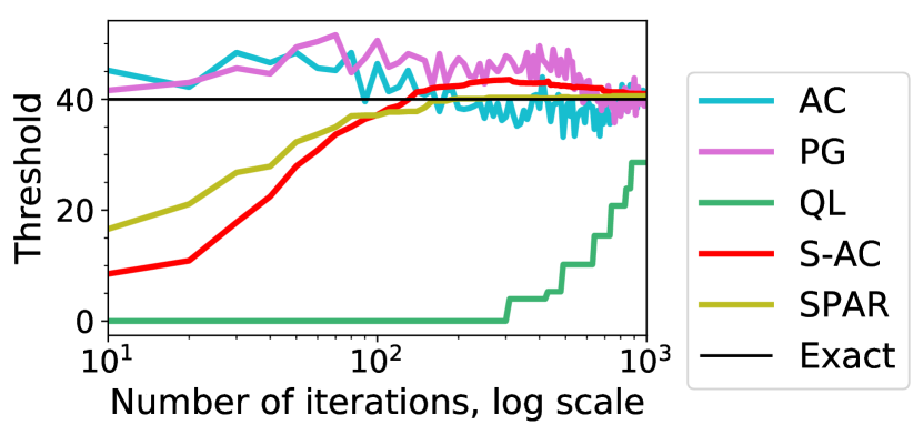
(c) $w_{0}=8$

Figure 6: Convergence of replenish-up-to thresholds at $t=0$ for the $R_{\textnormal{max}}=60,|\mathcal{W}|=9$ instance.

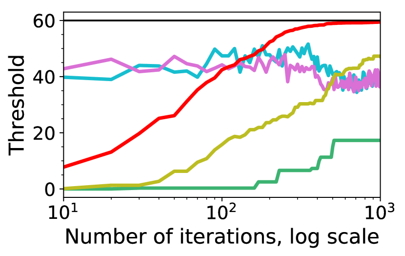
(a) $w_{0}=2$

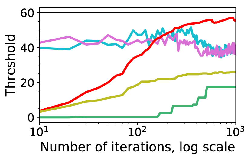
(b) $w_{0}=6$

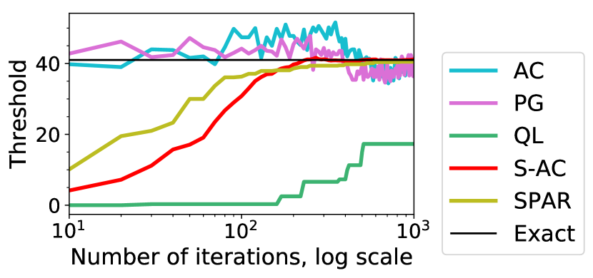
(c) $w_{0}=10$

Figure 7: Convergence of replenish-up-to thresholds at $t=0$ for the $R_{\textnormal{max}}=60,|\mathcal{W}|=12$ instance.

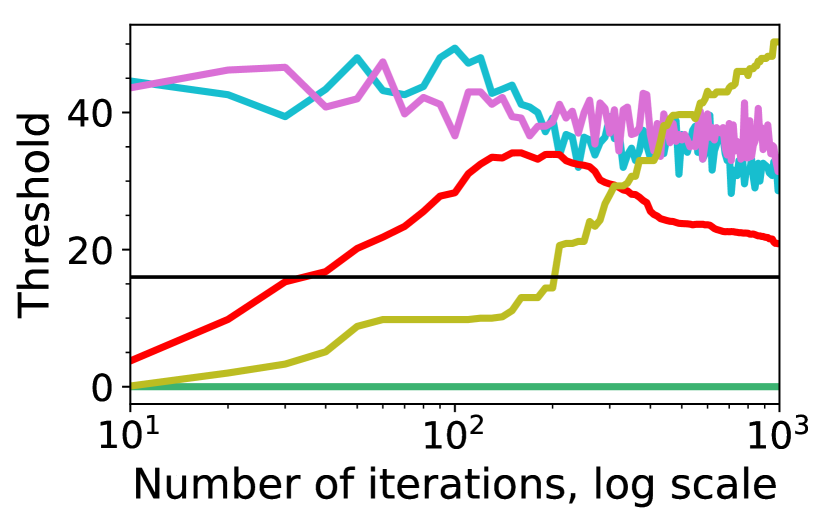
(a) $w_{0}=2$

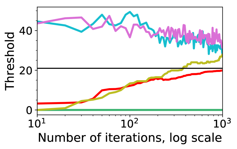
(b) $w_{0}=7$

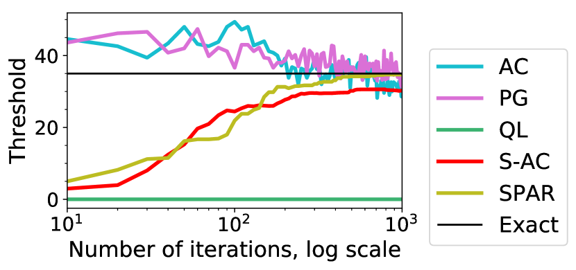
(c) $w_{0}=12$

Figure 8: Convergence of replenish-up-to thresholds at $t=0$ for the $R_{\textnormal{max}}=60,|\mathcal{W}|=15$ instance.

Convergence of Implied Basestock Thresholds

Next, we are interested in examining how the implied replenish-up-to thresholds evolve as each algorithm progresses. The thresholds of AC and PG are selected as the actions with highest probabilities for state $r=0$ and the thresholds of SPAR and QL correspond to the greedy policy with respect to the value function and state-action value function approximations. In this part, we take three problem instances as examples, whose storage capacities are all $R_{\textnormal{max}}=60$, and exogenous information spaces are $|\mathcal{W}|=9$, $|\mathcal{W}|=12$ and $|\mathcal{W}|=15$ respectively. Figures 6 to 8 show the convergence of approximate replenish-up-to threshold levels $\bar{l}^{\textnormal{rep},k}$ as well as the optimal levels $l^{\textnormal{rep}}$ (denoted “Exact” in the plots) for three different exogenous information states $w_{0}$ at period $t=0$ for the selected problem instances.

We see that the thresholds generated by S-AC quickly converge to the optimal ones in all instances. Due to the smoothing step of S-AC, the convergence is also observed to be relatively stable. On the other hand, the thresholds of AC, PG, QL, and SPAR tend to either have large gaps to the optimal thresholds or converge in a noisy manner. Stability of the basestock thresholds is particularly useful if S-AC is to be used in an online manner in practice, where drastic changes in the policy from one time period to the next (as observed in the competing algorithms) would be impractical. These results attest to the value of utilizing the structural properties of the policy and value function.

Sensitivity Analysis

In this section, we study the impact of model parameters. We take the instance with $R_{\textnormal{max}}=50$ and $|\mathcal{W}|=9$ in Section 6.1 as the base instance, and vary parameters in the model to evaluate the impact of each parameter. The results are summarized in Table 3. Each value in the table is an average of ten replications. For each replication, we take the policy learned by the algorithm at iteration 1,000 and evaluate it by averaging 100 simulations. The first parameter we are interested in is the demand distribution. We consider two types of distribution, normal and uniform distributions. For each type of distribution, we consider two values of the average demand of all PODs in a period, 30 and 50. The table shows that the value is highly influenced by the expected demand, and that with the same expected demand, the type of distribution has relatively little impact on the performance. We are also interested in the impact of the costs in the model. The ordering cost has a much larger impact than the holding cost, and any increase in the ordering cost can significantly reduce the value of the policy. We also note that S-AC finds near-optimal policies in each of these cases.

Table 3: Impact of parameters on ADP algorithms for the $R_{\textnormal{max}}=50,|\mathcal{W}|=9$ instance.

Parameter	Value	AC	PG	QL	S-AC	SPAR	Exact
Mean total demand	30, Normal	19,037	16,009	7,287	20,313	19,077	21,332
	30, Uniform	18,113	15,142	8,476	20,865	20,098	21,332
	50, Normal	28,422	23,237	10,318	29,080	28,278	29,387
	50, Uniform	28,023	23,112	10,286	29,077	28,150	29,387
Mean ordering cost	30	30,914	25,488	15,125	33,532	32,671	34,647
	50	18,037	14,009	7,287	20,313	19,077	20,689
	70	11,257	8,660	6,032	11,866	11,553	11,984
Holding cost	5	18,037	14,009	7,287	20,313	19,077	20,689
	20	18,402	15,064	7,189	19,839	19,285	20,131
	35	17,807	14,498	5,855	19,381	18,784	19,592
	50	17,150	15,011	4,582	18,988	18,418	19,203
	65	16,575	13,708	2,954	18,597	17,931	18,835

Case Study: Naloxone for First Responders in Pennsylvania

Our case study is motivated by the need to distribute naloxone (a drug that can reverse overdoses within seconds to minutes) amidst the ongoing opioid overdose crisis, which is affecting communities across the state of Pennsylvania. Our case study makes use a time-series demand model for naloxone, fit using publicly available data from Open Data Pennsylvania (2021). Our model in this section contains a five-dimensional information state $W_{t}$, which makes the standard version of S-AC intractable. Instead, we leverage an aggregation-based version of S-AC, whose details are introduced in Appendix C. In essence, the method uses clusters of the exogenous information state (via $k$-means clustering) and learns a cluster-dependent policy. When implementing the policy, we use regression to interpolate between clusters. Our experimental results show that this simple extension of S-AC for the case of a continuous and multi-dimensional information state is surprisingly effective.

Description of Naloxone for First Responders in Pennsylvania

The rate of opioid overdose deaths has quadrupled since 1999 (CDC, 2021d), with heroin deaths alone outpacing gun homicides in 2015 (Ingraham, 2016). Moreover, in 2015, drug overdose deaths in U.S. exceeded the combined mortalities from car accidents and firearms (Drug Enforcement Administration, 2015a; Drug Enforcement Administration, 2015b). By August 2020, the number of deaths from synthetic opioids was 52% more than the previous year (The Economist, 2021). There is significant benefit for drug users, family members, community members, law enforcement officers, and medical professionals alike to have training and access to the overdose reversal drug naloxone for use in risky situations (see Pennsylvania’s Act 139).

Table 4: Parameters used in the NFRP case study.

Parameter	Value	Meaning/Explanation
WTP/unit	$31,000	Willingness to pay (WTP) for a unit of naloxone. Product of the next 2 entries.
WTP/QALY	$50,000	WTP per quality-adjusted life-year (QALY) (Kaplan and Bush, 1982; Coffin and Sullivan, 2013).
QALY/unit	0.62	QALY adjustment factor for lives saved by naloxone. The average of utilities of “High-risk/low-risk prescription opioid use” and “Illicit opioid use” in Acharya et al. (2020).
Ordering cost	$185.30	Approximate retail price of an auto-injector form of naloxone (GoodRx, 2021).
Treatment cost	$2,976	The cost for EMS visit, EMS transport to hospital, and emergency department care (Coffin and Sullivan, 2013).
$R_{\textnormal{max}}$	700	Capacity of the central storage.
$h$	$10	Holding cost.
$b$	0	Disposal cost.

In this case study, we consider a somewhat simplified setting of a public health organization modeled after Naloxone for First Responders Program (NFRP), which distributes naloxone through a Centralized Coordination Entity (CCE). We use the top five counties in terms of overdose incidents responded to by emergency medical services (EMS) from publicly available data (Open Data Pennsylvania, 2021), Allegheny County, York County, Bucks County, Dauphin County, and Luzerne County (all of which have incident numbers over 1,000), as the five PODs (first responders) in our case study.

The parameters of our utility function are based on values found in Kaplan and Bush (1982), Coffin and Sullivan (2013), Acharya et al. (2020), and Open Data Pennsylvania (2021). Since the naloxone dispensed to first responders is used to reverse overdoses, we use willingness to pay (WTP) per unit of naloxone to measure the utility per demand satisfied. Specifically, let the WTP per unit of naloxone minus the treatment cost (EMS visit and related costs) be the unit utility $\Delta u$, similar to the approach taken by Coffin and Sullivan (2013). To reflect the different expected demand among counties, we adopt the following expected utility function in the case study: $u_{w}(y_{i},\xi_{i})=\Delta u\,\mathbf{E}_{w}\bigl{[}\min(y_{i},D_{i})\bigr{]}$, where $D_{i}$ is the demand of POD $i$. Further details (ordering cost, capacity of storage, and holding cost) are available in Table 4.

Figure 9: The hierarchical system structure used in the case study.

The system consists of an inventory control center, a dispensing coordinator, and multiple first responders as shown in Figure 9. Let the time horizon for the case study be $T=12$ months. At each period $t$, the inventory control center replenishes the inventory of naloxone after observing the recent incident history, modeled as the county-level incident count of the last period (thus, $W_{t}\in\mathbb{R}^{5}$). The control center then decides the total amount of naloxone to dispense in the current period. This naloxone is delivered to the CCE, who makes lower-level quantity-of-dispensing decisions based on the attribute of the arriving POD $\xi_{i}$, the current available naloxone in stock (the inventory level $x_{i}$), and the upper-level county-level incident count of the last period $W_{t}$. In the case study, the exogenous information is the incident history, which consists of the number of incidents from the five counties last month. We a vector autoregression (VAR) time-series model with a lag of 1.

Figure 10(a) shows the monthly number of overdose incidents in the five counties from January 1st, 2018 to July 31st, 2020, and 20 sample paths from the VAR(1) model for the next 24 months. The first planning period of the case study is July 2020. To generate the state aggregation, we sample 10,000 paths of the exogenous information, and use $k$-means clustering to cluster them into 12 clusters. Figure 10(b) shows the first three dimensions of the resulting clustering that is then used by S-AC.

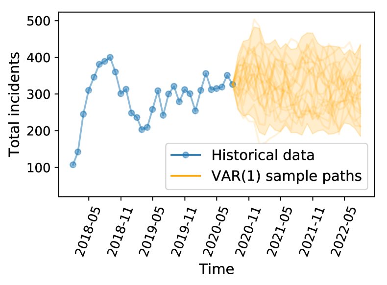
(a) Total number of incidents and predictions.

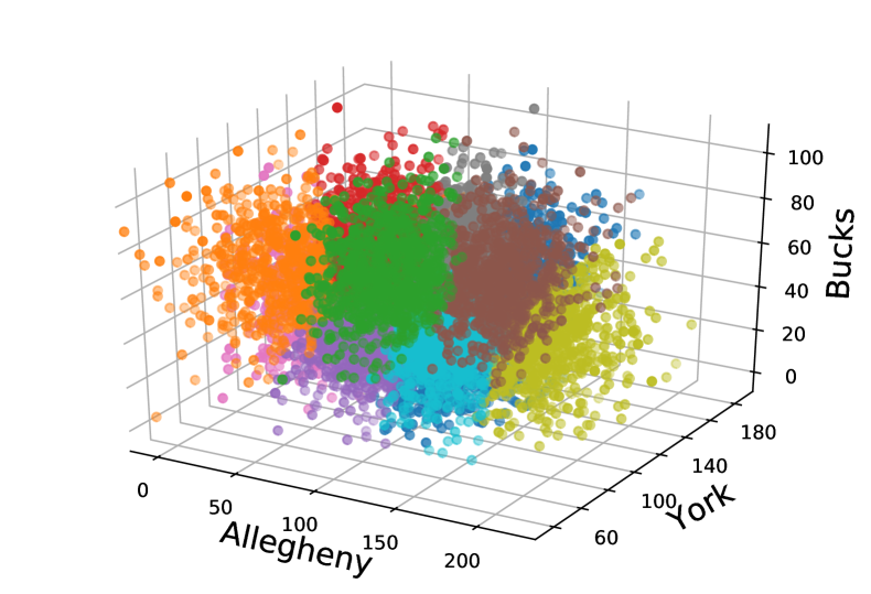
(b) Three dimensions of $k$-means clustering.

Figure 10: Total overdose incidents of the five PODs and $k$-means visualization.

Performance of the Algorithm

We denote the aggregate version of our algorithm S-AC+DPR, whose upper-level policies are learned by aggregate S-AC (see Appendix C). The learned cluster-dependent upper-level policies are then interpolated between clusters using Gaussian process regression. The lower-level policies are solved using a discretized DP we then interpolate using linear regression (DPR). In this section, we first study the performance of S-AC+DPR compared with AC+DPR and a suite of heuristic strategies. Next, we illustrate the impact of the various approaches on the lower-level dispensing decisions to each POD, showing some stark differences between the methods. Finally, we show some sensitivity analysis of the cost parameters on the value of the learned policies and heuristics.

Convergence and Comparison with Heuristics

We first describe the heuristic strategies to which we compare our new policy. We make a distinction between the upper-level and lower-level policies and consider two approaches for the upper-level and three approaches for the lower-level, resulting in six combined strategies. On the upper-level, we either take the S-AC policies (S-AC) or always replenish-up-to the expected demand and dispense-down-to zero (Mean). On the lower-level, the three strategies are: (1) take the policy trained using dynamic programming and interpolated to the continuous state space by linear regression (DPR), (2) evenly dispense naloxone to the five PODs (Even), and (3) follow the first-come-first-serve rule (FCFS), in which we dispense the expected demand of each POD upon its arrival until all the available resources are dispensed. We also apply AC+DPR as an alternative ADP method to which we can compare S-AC+DPR. We selected AC because it performs relatively well in Section 6 and is scalable to high-dimensional problems (unlike QL or SPAR).

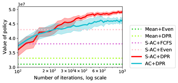
Figure 11: Convergence curve of S-AC and AC compared to performance of heuristics.

Figure 11 shows the cumulative performance of the policies over a year, averaged over 100 simulations (the value of policy Mean+FCFS is smaller than $3\mathrm{e}{7}$ and is removed from the plot to better show the results). We see that compared with the upper-level heuristic Mean, applying S-AC on the upper-level improves the performance (i.e., compare S-AC+DPR with Mean+DPR and S-AC+Even with Mean+Even). This is due to the ability of the state-dependent basestocks to adapt to dynamic state information. On the lower-level, we see that DPR outperforms the heuristics FCFS and Even (i.e., compare S-AC+DPR with S-AC+FCFS and S-AC+Even, and Mean+DPR with Mean+Even) significantly. The reason is that the heuristics FCFS dispensing policy is unable to take advantage of the large initial gains in dispensing resources to all of the first responders, and the heuristic Even dispensing policy is unable to adjust the dispensing decision to a POD based on exogenous information.

Figure 12: The relationship between total cost and total utility for each method.

Figure 12 shows the total cost vs. total utility for each method that we tested, which helps to illustrate the trade-offs associated with each. The total cost is mostly determined by the upper-level policy (i.e., the scatters of Mean+FCFS, Mean+Even and Mean+DPR are close on the x-axis, and the scatters of S-AC+FCFS, S-AC+Even and S-AC+DPR are close on the x-axis). The upper-level policy AC tends to always replenish the inventory up to a high level, which leads to the highest total cost. The heuristics Mean considers the exogenous information by always replenishing up to the expected demand and dispense all the inventory to the PODs; this approach leads to the lowest total cost. The upper-level policy learned by S-AC is able to adapt to the exogenous information state and usually replenishes up to a level that is higher than the expected demand. It also sometimes retains a small portion of the inventory to the next period. With the same upper-level policy, although the total cost is similar, the total utility differs when applying different lower-level policy. This observation suggests that by applying a smarter lower-level policy DPR, it is possible to achieve more utility without spending much more cost. Overall, we see that our primary approach S-AC+DPR attains the highest levels of utility while expending relatively moderate cost.

Utilities of Different First Responders

We now investigate the individual POD (or first responder) utilities achieved under each algorithm. Following the policy obtained after $1,000$ iterations of S-AC+DPR, we get the total utility of each POD during the entire planning horizon. Under our utility function definition and the parameters given in Table 4, the PODs with higher levels of overdose incidents are associated with a higher utilities than PODs fewer incidents. Thus, we expect that a good inventory and dispensing policy will learn to prioritize these high-utility PODs. Figure 13 shows the histograms of 1,000 simulations for the utilities of the five PODs alongside the historical county-level overdose incidents.

(a) County-level overdose incidents.

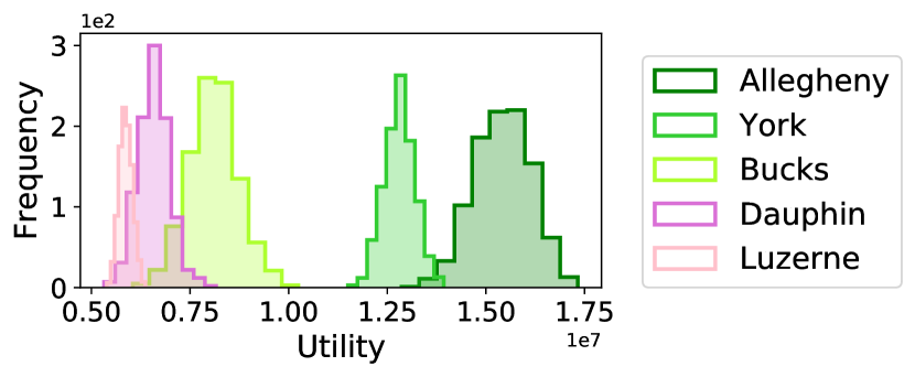
(b) Cumulative utilities achieved by S-AC+DPR.

Figure 13: Historical overdose incidents by county and the prioritization learned by S-AC+DPR

To investigate how each method prioritizes the different PODs, we show the utilities of each POD generated by each policy in Figure 14. S-AC+DPR leads to the highest utilities of the first three counties, while S-AC+Even leads to the highest utility of the last county. These two policies perform similarly for the fourth county. Moreover, the two ADP algorithms S-AC+DPR and AC+DPR are in the top three policies for all of the counties’ utilities.

(a) Allegheny

(b) York

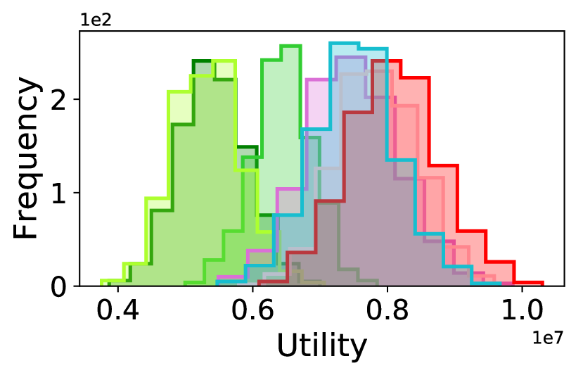
(c) Bucks

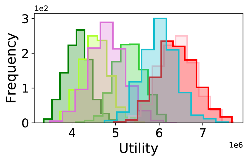
(d) Dauphin

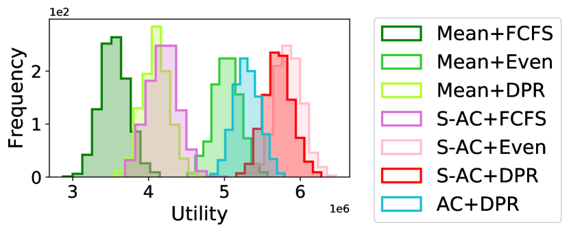
(e) Luzerne

Figure 14: Comparison of the cumulative utilities for each method.

When both levels’ policies are heuristics (i.e., Mean+FCFS and Mean+Even), the utility of all PODs are low, with Mean+FCFS leading to the lowest utilities in all cases. When only the upper-level is a heuristic (i.e., Mean+DPR), the utilities are still not particularly high; in fact, this method ranks in the bottom three policies for all the PODs except for Allegheny. When the upper-level is S-AC and the lower-level is a heuristic (i.e., S-AC+FCFS and S-AC+Even), the utilities of the top three counties are higher than the utilities by achieved using Mean. The policy S-AC+Even never falls in the bottom three policies; S-AC+FCFS performs reasonably but is part of the bottom three policies for Dauphin and Luzerne. In summary, both the upper-level and the lower-level policies play an important in this problem: a properly designed lower-level heuristic can achieve good utility values for some of the PODs; however, intelligent policies on both the upper and lower-levels is necessary to achieve the overall improvement.

Ordering Cost Sensitivity Analysis

Table 5 shows the effect of the ordering cost on the performance (in terms of value achieved) of the various algorithms. The other costs (holding cost and disposal cost) exhibited very minor effects on the value and thus we omitted the results. Each value in the table is an average of twenty replications of the algorithm, and for each replication of the ADP algorithms, S-AC+DPR and AC+DPR, we take the policy learned by the algorithm at iteration 1,000 and evaluate it by averaging 100 simulations. The table shows that S-AC+DPR outperforms the other approaches in all settings. When the ordering cost increases to 5 times (increases from 185 to 925), the value of S-AC+DPR decreases 9.35%, and when it increases to 20 times (increases from 185 to 3,700), the value decreases 42.48%. These results indicate that the ordering cost of naloxone has a significant influence on the operations of a public health department.

Table 5: Simulated value of the policies on instances with different ordering costs (value in 10 million).

Ordering cost	Mean+FCFS	Mean+Even	Mean+DPR	S-AC+FCFS	S-AC+Even	S-AC+DPR	AC+DPR
185	2.07	3.10	3.31	3.81	4.30	4.92	4.64
925	1.94	2.96	3.39	3.70	4.10	4.46	4.34
1,850	1.75	2.77	3.04	3.12	3.56	3.92	3.76
3,700	1.39	2.41	2.00	2.06	2.62	2.83	2.56

Extensions

We showed how an aggregation-based version of S-AC along with $k$-means clustering can be used to handle the multi-dimensional continuous features used in the case study. There are also other possible extensions to S-AC that can make it more scalable to high-dimensional problems. For example, shape-constrained deep neural networks Gupta et al. (2019) Gupta et al. (2021) can handle both monotonicity and concavity via penalization of derivatives during training. In principle, our S-AC algorithm could be extended to use techniques like these, but the same core principles of S-AC would remain intact. We leave these investigations to future work.

Conclusions

In this paper, we formulate a hierarchical MDP model for the sequential problem of optimizing inventory control and making dispensing decisions for a public health organization. We propose a novel, provably convergent actor-critic algorithm that utilizes problem structure in both the policy and value approximations (state-dependent basestock structure for the policy and concavity for the value functions). Although the algorithm is developed in the setting of our specific MDP, the general paradigm of a structured actor-critic algorithm is likely to be of broader methodological interest. Numerical experiments show that high-quality policies can be obtained in a small number of iterations and that the convergence of the policy is significantly less noisy when compared to competing algorithms. Lastly, we propose an aggregation-based version of our algorithm and provide a case study for the problem of dispensing naloxone to first responders.

Appendix A Proofs

In this section, we give the proofs of results from the main paper: Proposition 2, Lemma 1, and Theorem 1.

Proof of Proposition 1

We prove the $L^{\natural}$-concavity of the $Q$-value function of the lower-level problem by backward induction. Note that if this is true, then the discrete concavity of $U_{w,i}(x,\xi)$ in $x$ follows by Lemma 2 of Chen et al. (2014). Let $J_{w,i}(x,\xi,y)$ be the $Q$-value for a given state-action pair $(x,\xi,y)$ at period $i$:

$$J_{w,i}(x,\xi,y)=u_{w}\bigl{(}y,\xi\bigr{)}+\mathbf{E}_{w}\bigl{[}U_{w,i+1}(X_{i+1},\Xi_{i+1})\bigr{]}.$$

The base case is $J_{w,n+1}(x,\xi,y)=b\,x$, which is $L^{\natural}$-concave in $(x,y)$. The induction hypothesis is that $J_{w,i+1}(x,\xi,y)$ is $L^{\natural}$-concave in $(x,y)$.

We analyze $J_{w,i}(x,\xi,y)$ by breaking it up into two terms. The first term is $L^{\natural}$-concave in $y$ according to Assumption 1. The second term $U_{w,i+1}(X_{i+1},\Xi_{i+1})$ is $L^{\natural}$-concave in $X_{i+1}$ according to Lemma 2 of Chen et al. (2014). Since $X_{i+1}=x-y$, $U_{w,i+1}(X_{i+1},\Xi_{i+1})$ is $L^{\natural}$-concave in $(x,y)$ by Lemma 2 in Zipkin (2008b). This concludes the proof.

Proof of Proposition 2

First, we prove part 1. Let us define the state-action value function (or the $Q$-value). The terminal value is defined as $Q_{T}^{\textnormal{rep}}(r,w;z^{\textnormal{rep}})=-b\,r$. For $t<T$, replenish-up-to decision $z^{\textnormal{rep}}\in\bar{\mathcal{Z}}(r)$, and dispense-down-to decision $z^{\textnormal{dis}}\in\underline{\mathcal{Z}}(z^{\textnormal{rep}})$,

$$Q_{t}^{\textnormal{rep}}(r,w;z^{\textnormal{rep}})=(c_{w}-h)\,r-c_{w}z^{\textnormal{rep}}+V_{t}^{\textnormal{dis}}(z^{\textnormal{rep}},w),$$ (21)

$$Q_{t}^{\textnormal{dis}}(z^{\textnormal{rep}},w;z^{\textnormal{dis}})=\mathbf{E}_{w}\bigl{[}U_{w,0}\bigl{(}z^{\textnormal{rep}}-z^{\textnormal{dis}},\Xi_{t,0}\bigr{)}+V_{t+1}^{\textnormal{rep}}(R_{t+1},W_{t+1})\bigr{]},$$ (22)

where $R_{t+1}=z^{\textnormal{dis}}$. We now prove the $L^{\natural}$-concavity of $Q$-value by backward induction. Note that if this is true, then the $L^{\natural}$-concavity of $\tilde{V}_{t}^{\textnormal{rep}}$ and $\tilde{V}_{t}^{\textnormal{dis}}$ follows. The base case is $Q_{T}^{\textnormal{rep}}(r,w;z^{\textnormal{rep}})=-b\,r$, which is $L^{\natural}$-concave in $(r,z^{\textnormal{rep}})$, and the induction hypothesis is the same property for $Q_{t+1}^{\textnormal{rep}}(r,w;z^{\textnormal{rep}})$.

We first analyze (22) by breaking it up into two terms. The first term $\mathbf{E}_{w}\bigl{[}U_{w,0}\bigl{(}z^{\textnormal{rep}}-z^{\textnormal{dis}},\Xi_{t,0}\bigr{)}\bigr{]}$ is discretely concave in $(z^{\textnormal{rep}},z^{\textnormal{dis}})$ according to Proposition 1 and Lemma 2 in Zipkin (2008b). In the second term, $V_{t+1}^{\textnormal{rep}}(r,w)=\max_{z^{\textnormal{rep}}\in\bar{\mathcal{Z}}(r)}Q_{t+1}^{\textnormal{rep}}(r,w;z^{\textnormal{rep}})$. Lemma 2 of Chen et al. (2014) shows that $V_{t+1}^{\textnormal{rep}}(r,w)$ is $L^{\natural}$ concave in $r$. Since $R_{t+1}=z^{\textnormal{dis}}$, the term $V_{t+1}^{\textnormal{rep}}(R_{t+1},W_{t+1})$ is $L^{\natural}$-concave in $z^{\textnormal{dis}}$. $L^{\natural}$-concavity is preserved under expectations, so $Q_{t}^{\textnormal{dis}}(z^{\textnormal{rep}},w;z^{\textnormal{dis}})$ is $L^{\natural}$-concave in $(z^{\textnormal{rep}},z^{\textnormal{dis}})$.

Next, we analyze (21) by breaking it up into two terms. The first term $(c_{w}-h)\,r-c_{w}z^{\textnormal{rep}}$ is clearly $L^{\natural}$-concave in $(r,z^{\textnormal{rep}})$. The second term $V_{t}^{\textnormal{dis}}(z^{\textnormal{rep}},w)=\max_{z^{\textnormal{dis}}\in\underline{\mathcal{Z}}(z^{\textnormal{rep}})}Q_{t}^{\textnormal{dis}}(z^{\textnormal{rep}},w;z^{\textnormal{dis}})$. Lemma 2 of Chen et al. (2014) shows that $V_{t}^{\textnormal{dis}}(z^{\textnormal{rep}},w)$ is $L^{\natural}$ concave in $z^{\textnormal{rep}}$. This concludes Part 1.

Proof of Lemma 1

Let us show part (1), the convergence of $\bar{v}_{t}^{\textnormal{rep},k}(z^{\textnormal{rep}},w)$. The convergence of $\bar{v}_{t}^{\textnormal{dis},k}(z^{\textnormal{dis}},w)$ in part (2) of the lemma is similar. Since the demand $D_{t,i}$ is bounded by $D_{\textnormal{max}}$, there exists a $v_{\text{max}}^{\textnormal{rep}}>0$ such that $|v_{t}^{\textnormal{rep}}(z^{\textnormal{rep}},w)|\leq v_{\text{max}}^{\textnormal{rep}}$ for all $t$, $z^{\textnormal{rep}}$, and $w$. We first construct two deterministic sequences $\{G^{m}\}$ and $\{I^{m}\}$ such that $G^{0}=v^{\textnormal{rep}}+v_{\text{max}}^{\textnormal{rep}}$ and $I^{0}=v^{\textnormal{rep}}-v_{\text{max}}^{\textnormal{rep}}$ with

$$G^{m+1}=\frac{G^{m}+v^{\textnormal{rep}}}{2}\quad\text{and}\quad I^{m+1}=\frac{I^{m}+v^{\textnormal{rep}}}{2}.$$ (23)

It is easy to show that

$$G^{m}\rightarrow v^{\textnormal{rep}}\quad\text{and}\quad I^{m}\rightarrow v^{\textnormal{rep}}.$$ (24)

Our goal in this proof is to show that for any $m$ and sufficiently large $k$,

$$I_{t}^{m}(z^{\textnormal{rep}},w)\leq\bar{v}_{t}^{\textnormal{rep},k-1}(z^{\textnormal{rep}},w)\leq G_{t}^{m}(z^{\textnormal{rep}},w).$$ (25)

If (25) is true, then we can conclude the result of Lemma 1 by (24).

We now introduce a random set of states $\mathcal{S}_{t}^{-}$ that are increased by the projection operator (19) on finitely many iterations $k$. Formally, let

$$\mathcal{S}_{t}^{-}=\bigl{\{}(z^{\textnormal{rep}},w)\in\mathcal{S}:\tilde{v}_{t}^{\textnormal{rep},k}(z^{\textnormal{rep}},w)<\bar{v}_{t}^{\textnormal{rep},k}(z^{\textnormal{rep}},w)\;\;\text{finitely often}\bigr{\}}.$$

Let $\bar{K}$ be the random variable that describes the iteration number after which states in $\mathcal{S}_{t}^{-}$ are no longer increased by the projection step; i.e., for all $(z^{\textnormal{rep}},w)\in\mathcal{S}_{t}^{-}$, it holds that $\tilde{v}_{t}^{\textnormal{rep},k}(z^{\textnormal{rep}},w)\geq\bar{v}_{t}^{\textnormal{rep},k}(z^{\textnormal{rep}},w)$ for all $k\geq\bar{K}$. We break apart (25) into two separate inequalities; this proof will focus on showing that for a fixed $m$, there exists a finite random index $\hat{K}_{t}^{m}$ such that for all $k\geq\hat{K}_{t}^{m}$,

$$\bar{v}_{t}^{\textnormal{rep},k-1}(z^{\textnormal{rep}},w)\leq G_{t}^{m}(z^{\textnormal{rep}},w).$$ (26)

The state space $\mathcal{S}$ can be partitioned into two parts: (1) states $(z^{\textnormal{rep}},w)\in\mathcal{S}^{-}_{t}$ and (2) states $(z^{\textnormal{rep}},w)\in\mathcal{S}\setminus\mathcal{S}_{t}^{-}$. The proof of (26) will consider each partition separately. We now define some noise terms and stochastic sequences. Recall from (15) and (17) that $\hat{v}_{t}^{\textnormal{rep},k}=\hat{V}_{t}^{\textnormal{rep},k}(z_{t}^{\textnormal{rep},k},w_{t}^{k})-\hat{V}_{t}^{\textnormal{rep},k}(z_{t}^{\textnormal{rep},k}-1,w_{t}^{k})$, where

$$\hat{V}_{t}^{\textnormal{rep},k}(z^{\textnormal{rep}},w_{t}^{k})= -c_{w_{t}^{k}}z^{\textnormal{rep}}+U_{w_{t}^{k},0}^{\mu^{*}}\bigl{(}z^{\textnormal{rep}}-\tilde{\pi}_{t}^{\textnormal{dis},k-1}(z^{\textnormal{rep}},w_{t}^{k}),\check{\xi}_{t,0}^{k}\bigr{)}$$

$$+f_{t}^{\textnormal{dis}}\bigl{(}\tilde{\pi}^{\textnormal{rep},k-1},\tilde{\pi}^{\textnormal{dis},k-1};\mathbf{Z}^{k}_{t}(w_{t}),z^{\textnormal{rep}}\bigr{)},$$

By our assumption that $\mkern 1.5mu\overline{\mkern-0.5mul\mkern-0.5mu}\mkern 1.5mu_{\tau}^{\textnormal{rep},k}(w)\rightarrow l_{\tau}^{\textnormal{rep}}(w)$ almost surely for $\tau\geq t+1$, and $\mkern 1.5mu\overline{\mkern-0.5mul\mkern-0.5mu}\mkern 1.5mu_{\tau}^{\textnormal{dis},k}(w)\rightarrow l_{\tau}^{\textnormal{dis}}(w)$ almost surely for $\tau\geq t$, and the fact that $f_{t}^{\textnormal{dis}}\bigl{(}\tilde{\pi}^{\textnormal{rep},k-1},\tilde{\pi}^{\textnormal{dis},k-1};\mathbf{Z}^{k}_{t}(w_{t}),z^{\textnormal{rep}}\bigr{)}$ depends only on the replenish-up-to thresholds for periods $t+1$ onward and the dispense-down-to thresholds for periods $t$ onward, it follows that the simulated value of $\tilde{\pi}^{\textnormal{rep},k-1}$ and $\tilde{\pi}^{\textnormal{dis},k-1}$ becomes unbiased asymptotically:

$$\mathbf{E}_{w}\bigl{[}f_{t}^{\textnormal{dis}}\bigl{(}\tilde{\pi}^{\textnormal{rep},k-1},\tilde{\pi}^{\textnormal{dis},k-1};\mathbf{Z}^{k}_{t}(w),z^{\textnormal{rep}}\bigr{)}\bigr{]}\rightarrow\tilde{V}_{t}^{\textnormal{dis}}\bigl{(}\pi_{t}^{\textnormal{dis},*}(z^{\textnormal{rep}},w),w\bigr{)}\quad\text{a.s.}$$ (27)

We define the noise term $\epsilon_{t}^{k}(z_{t}^{\textnormal{rep},k},w_{t}^{k})$ such that

$$\epsilon_{t}^{k}(z_{t}^{\textnormal{rep},k},w_{t}^{k})=\mathbf{E}\bigl{[}\hat{v}_{t}^{\textnormal{rep},k}\bigr{]}-v_{t}^{\textnormal{rep}}(z_{t}^{\textnormal{rep},k},w_{t}^{k}).$$ (28)

Note that we can conclude from (27) that $\epsilon_{t}^{k}(z_{t}^{\textnormal{rep},k},w_{t}^{k})\rightarrow 0$ almost surely. We define another noise term $\varepsilon_{t}^{k}(z_{t}^{\textnormal{rep},k},w_{t}^{k})$ such that $\varepsilon_{t}^{k}(z_{t}^{\textnormal{rep},k},w_{t}^{k})=\hat{v}_{t}^{\textnormal{rep},k}-\mathbf{E}\bigl{[}\hat{v}_{t}^{\textnormal{rep},k}\bigr{]}$. Thus, we can see that

$$\hat{v}_{t}^{\textnormal{rep},k}=v_{t}^{\textnormal{rep}}(z_{t}^{\textnormal{rep},k},w_{t}^{k})+\epsilon_{t}^{k}(z_{t}^{\textnormal{rep},k},w_{t}^{k})+\varepsilon_{t}^{k}(z_{t}^{\textnormal{rep},k},w_{t}^{k})$$ (29)

Next, we need to define some stochastic sequences related to these noise terms. Let $\{\bar{s}_{t}^{k}\}$ be defined such that for $k<\bar{K}$, $\bar{s}_{t}^{k}(z^{\textnormal{rep}},w)=0$, and for $k\geq\bar{K}$,

$$\bar{s}_{t}^{k}(z^{\textnormal{rep}},w)=\bigl{(}1-\alpha_{t}^{k}(z^{\textnormal{rep}},w)\bigr{)}\,\bar{s}_{t}^{k-1}(z^{\textnormal{rep}},w)+\alpha_{t}^{k}(z^{\textnormal{rep}},w)\bigl{[}\epsilon_{t}^{k}(z_{t}^{\textnormal{rep},k},w_{t}^{k})+\varepsilon_{t}^{k}(z_{t}^{\textnormal{rep},k},w_{t}^{k})\bigr{]}.$$ (30)

This sequence averages both of the noise terms. Since $\epsilon_{t}^{k}$ is unbiased and $\varepsilon_{t}^{k}$ converges to zero, we can apply Theorem 2.4 of Kushner and Yin (2003), a standard stochastic approximation convergence result, to conclude that $\bar{s}_{t}^{k}(z^{\textnormal{rep}},w)\rightarrow 0$ almost surely. We then define a stochastic bounding sequence $\{\bar{g}_{t}\}$ such that for $k<\bar{K}$, $\bar{g}_{t}^{k}(z^{\textnormal{rep}},w)=G_{t}^{k}(z^{\textnormal{rep}},w)$ and for $k\geq\bar{K}$,

$$\bar{g}_{t}^{k}(z^{\textnormal{rep}},w)=\bigl{(}1-\alpha_{t}^{k}(z^{\textnormal{rep}},w)\bigr{)}\,\bar{g}_{t}^{k-1}(z^{\textnormal{rep}},w)+\alpha_{t}^{k}(z^{\textnormal{rep}},w)\,v_{t}^{\textnormal{rep}}(z^{\textnormal{rep}},w).$$ (31)

Part (1).

As in Nascimento and Powell (2009), we provide an $\omega$-wise argument, meaning that we consider a fixed $\omega\in\Omega$ (although the dependence of random variables on $\omega$ is omitted for notational simplicity). Here, we show the existence of a finite index $\tilde{K}_{t}^{m}$ such that for all states $(z^{\textnormal{rep}},w)\in\mathcal{S}^{-}_{t}$, it holds that for all iterations $k\geq\tilde{K}_{t}^{m}$, $\bar{v}_{t}^{\textnormal{rep},k-1}(z^{\textnormal{rep}},w)\leq G_{t}^{m}(z^{\textnormal{rep}},w)$. The proof is a forward induction on $m$ where the base case is $m=0$. The base case can be easily proved by applying the definition of $G^{0}$ (note that we can select $\tilde{K}_{t}^{m}\geq\bar{K}$. The induction hypothesis is that there exists an integer $\tilde{K}_{t}^{m}\geq\bar{K}$ such that for all $k\geq\tilde{K}_{t}^{m}$, the inequality (26) is true. The next step is $m+1$: we must show the existence of an integer $\tilde{K}_{t}^{m+1}\geq\bar{K}$ such that for all states $(z^{\textnormal{rep}},w)\in\mathcal{S}^{-}_{t}$, it holds that

$$\bar{v}_{t}^{\textnormal{rep},k-1}(z^{\textnormal{rep}},w)\leq G_{t}^{m+1}(z^{\textnormal{rep}},w)$$ (32)

for all iterations $k\geq\tilde{K}_{t}^{m+1}$. We require the following lemma.

Lemma 2.

The inequality

$$\bar{v}_{t}^{\textnormal{rep},k-1}(z^{\textnormal{rep}},w)\leq\bar{g}_{t}^{k-1}(z^{\textnormal{rep}},w)+\bar{s}_{t}^{k-1}(z^{\textnormal{rep}},w)$$ (33)

holds almost everywhere on $\{k\geq\tilde{K}_{t}^{m},\;(z^{\textnormal{rep}},w)\in\mathcal{S}^{-}_{t}\}$.

Proof.

When $k=\tilde{K}_{t}^{m}$, the relationship (33) can be shown using the definitions of $\bar{g}_{t}^{k-1}(z^{\textnormal{rep}},w)$ and $\bar{s}_{t}^{k-1}(z^{\textnormal{rep}},w)$, along with the induction hypothesis (26). We now induct on $k$. Suppose that (33) is true for a given $k\geq\tilde{K}_{t}^{m}$. The inductive step is to show $\bar{v}_{t}^{\textnormal{rep},k}(z^{\textnormal{rep}},w)\leq\bar{g}_{t}^{k}(z^{\textnormal{rep}},w)+\bar{s}_{t}^{k}(z^{\textnormal{rep}},w)$. To simplify notation, let $\check{\alpha}_{t}^{k}$, $\check{v}_{t}^{k}$, $\check{s}_{t}^{k}$, and $\check{g}_{t}^{k}$ respectively denote $\alpha_{t}^{k}(z^{\textnormal{rep}},w)$, $\bar{v}_{t}^{\textnormal{rep},k}(z^{\textnormal{rep}},w)$, $\bar{s}_{t}^{k}(z^{\textnormal{rep}},w)$ and $\bar{g}_{t}^{k}(z^{\textnormal{rep}},w)$. For state $(z^{\textnormal{rep}},w)=(z_{t}^{\textnormal{rep},k},w_{t}^{k})$, we have

$$\check{v}_{t}^{k} =\tilde{v}_{t}^{\textnormal{rep},k}(z^{\textnormal{rep}},w)=(1-\check{\alpha}_{t}^{k})\check{v}_{t}^{k-1}+\check{\alpha}_{t}^{k}\hat{v}_{t}^{\textnormal{rep},k}$$

$$\leq(1-\check{\alpha}_{t}^{k})\bigl{(}\check{g}_{t}^{k-1}+\check{s}_{t}^{k-1}\bigr{)}+\check{\alpha}_{t}^{k}\hat{v}_{t}^{\textnormal{rep},k}-\check{\alpha}_{t}^{k}v_{t}^{\textnormal{rep}}(z_{t}^{\textnormal{rep},k},w_{t}^{k})+\check{\alpha}_{t}^{k}v_{t}^{\textnormal{rep}}(z_{t}^{\textnormal{rep},k},w_{t}^{k})$$

$$=(1-\check{\alpha}_{t}^{k})\bigl{(}\check{g}_{t}^{k-1}+\check{s}_{t}^{k-1}\bigr{)}+\check{\alpha}_{t}^{k}\bigl{[}\epsilon_{t}^{k}(z_{t}^{\textnormal{rep},k},w_{t}^{k})+\varepsilon_{t}^{k}(z_{t}^{\textnormal{rep},k},w_{t}^{k})\bigr{]}+\check{\alpha}_{t}^{k}v_{t}^{\textnormal{rep}}(z_{t}^{\textnormal{rep},k},w_{t}^{k})$$

$$=(1-\check{\alpha}_{t}^{k})\check{g}_{t}^{k-1}+\check{s}_{t}^{k}+\check{\alpha}_{t}^{k}v_{t}^{\textnormal{rep}}(z_{t}^{\textnormal{rep},k},w_{t}^{k})$$

$$=\check{g}_{t}^{k}+\check{s}_{t}^{k}.$$

The first equality is due to the fact that $(z^{\textnormal{rep}},w)=(z_{t}^{\textnormal{rep},k},w_{t}^{k})$, which is unaltered by the projection operator (19). The second inequality follows from the induction hypothesis (33). The last three steps follow by (29), (30) and (31) respectively.

For $(z^{\textnormal{rep}},w)\neq(z_{t}^{\textnormal{rep},k},w_{t}^{k})$, which are the states that are not updated by a direct observation of the sample slope at iteration $k$, period $t$, the stepsize $\check{\alpha}_{t}^{k}=0$. Then, we have

$$\check{s}_{t}^{k}=\check{s}_{t}^{k-1}\quad\text{and }\quad\check{g}_{t}^{k}=\check{g}_{t}^{k-1}.$$

Therefore, from the definition of set $\mathcal{S}^{-}_{t}$, the fact that $\tilde{K}_{t}^{m}\geq\bar{K}$, and the induction hypothesis, we have

$$\check{v}_{t}^{k}\leq\tilde{v}_{t}^{\textnormal{rep},k}(z^{\textnormal{rep}},w)=\check{v}_{t}^{k-1}\leq\check{g}_{t}^{k-1}+\check{s}_{t}^{k-1}=\check{g}_{t}^{k}+\check{s}_{t}^{k},$$

which concludes the proof of (33). ∎

Since $G^{m}\geq G^{m+1}\geq v^{\textnormal{rep}}$ for all $m$, when $G_{t}^{m}(z^{\textnormal{rep}},w)=v_{t}^{\textnormal{rep}}(z^{\textnormal{rep}},w)=G_{t}^{m+1}(z^{\textnormal{rep}},w)$, the inequality $\bar{v}_{t}^{\textnormal{rep},k-1}(z^{\textnormal{rep}},w)\leq G_{t}^{m}(z^{\textnormal{rep}},w)$ implies that $\bar{v}_{t}^{\textnormal{rep},k-1}(z^{\textnormal{rep}},w)\leq G_{t}^{m+1}(z^{\textnormal{rep}},w)$. Thus, the only remaining states to consider are the ones where $G_{t}^{m}(z^{\textnormal{rep}},w)>v_{t}^{\textnormal{rep}}(z^{\textnormal{rep}},w)$. Let $\delta^{m}$ be the minimum of the quantity $[G_{t}^{k}(z^{\textnormal{rep}},w)-v_{t}^{\textnormal{rep}}(z^{\textnormal{rep}},w)]/4$ over states $(z^{\textnormal{rep}},w)\in\mathcal{S}_{t}^{-}$ with $G_{t}^{m}(z^{\textnormal{rep}},w)>v_{t}^{\textnormal{rep}}(z^{\textnormal{rep}},w)$. Define an integer $K^{G}\geq\tilde{K}_{t}^{m}$ such that for all states $(z^{\textnormal{rep}},w)\in\mathcal{S}^{-}_{t}$,

$$\textstyle\prod_{k=\tilde{K}_{t}^{m}}^{K^{G}-1}\bigl{(}1-\alpha_{t}^{k}(z^{\textnormal{rep}},w)\bigr{)}\leq 1/4\quad\text{and}\quad\bar{s}_{t}^{k}(z^{\textnormal{rep}},w)\leq\delta^{m}.$$

for every iteration $k\geq K^{G}$. We can find such a $K^{G}$ because the stepsize conditions of Assumption 2 imply that

$$\textstyle\prod_{k=\tilde{K}_{t}^{m}}^{\infty}\bigl{(}1-\alpha_{t}^{k}(z^{\textnormal{rep}},w)\bigr{)}=0,$$

and because $\bar{s}_{t}^{k}(z^{\textnormal{rep}},w)$ converges to zero.

Now we are ready to show (32). The definition of the sequence $\{\bar{g}_{t}^{k}\}$ implies that $\bar{g}_{t}^{k}(z^{\textnormal{rep}},w)$ is a convex combination of $G_{t}^{k}(z^{\textnormal{rep}},w)$ and $v_{t}^{\textnormal{rep}}(z^{\textnormal{rep}},w)$, of the form

$$\bar{g}_{t}^{k}(z^{\textnormal{rep}},w)=\hat{\alpha}_{t}^{k}(z^{\textnormal{rep}},w)\,G_{t}^{k}(z^{\textnormal{rep}},w)+\bigl{(}1-\hat{\alpha}_{t}^{k}(z^{\textnormal{rep}},w)\bigr{)}\,v_{t}^{\textnormal{rep}}(z^{\textnormal{rep}},w),$$

where $\hat{\alpha}_{t}^{k}(z^{\textnormal{rep}},w)=\prod_{k=\tilde{K}_{t}^{m}}^{K-1}\bigl{(}1-\alpha_{t}^{k}(z^{\textnormal{rep}},w)\bigr{)}\leq 1/4$ for $k\geq K^{G}$. Because $G^{m}\geq v^{\textnormal{rep}}$ for any $m$, it follows that

$$\bar{g}_{t}^{k}(z^{\textnormal{rep}},w) \leq\textstyle\frac{1}{4}\,G_{t}^{k}(z^{\textnormal{rep}},w)+\frac{3}{4}\,v_{t}^{\textnormal{rep}}(z^{\textnormal{rep}},w)$$

$$=\textstyle\frac{1}{2}\,G_{t}^{k}(z^{\textnormal{rep}},w)+\frac{1}{2}\,v_{t}^{\textnormal{rep}}(z^{\textnormal{rep}},w)-\frac{1}{4}\,\bigl{(}G_{t}^{k}(z^{\textnormal{rep}},w)-v_{t}^{\textnormal{rep}}(z^{\textnormal{rep}},w)\bigr{)}$$

$$\leq G_{t}^{k+1}(z^{\textnormal{rep}},w)-\delta^{m},$$

where the second inequality follows from (23) and the definition of $\delta^{m}$. Recall that we are concentrating on the case where $G_{t}^{m}(z^{\textnormal{rep}},w)>v_{t}^{\textnormal{rep}}(z^{\textnormal{rep}},w)$, so $\delta^{m}$ is well-defined and positive. This inequality, together with Lemma 2 and $\bar{s}_{t}^{k}(z^{\textnormal{rep}},w)\leq\delta^{m}$, imply that for all $k\geq K^{G}$,

$$\bar{g}_{t}^{k}(z^{\textnormal{rep}},w)\leq G_{t}^{k+1}(z^{\textnormal{rep}},w)-\delta^{m}+\bar{s}_{t}^{k}(z^{\textnormal{rep}},w)\leq G_{t}^{k+1}(z^{\textnormal{rep}},w)-\delta^{m}+\delta^{m}\leq G_{t}^{k+1}(z^{\textnormal{rep}},w).$$

We conclude Part (1) of the proof by letting $\tilde{K}_{t}^{m+1}=K^{G}$.

Part (2).

We now focus on the states $(z^{\textnormal{rep}},w)\in\mathcal{S}\setminus\mathcal{S}^{-}_{t}$ that are increased infinitely often. For a fixed $m$ and state $(z^{\textnormal{rep}},w)\in\mathcal{S}\setminus\mathcal{S}^{-}_{t}$, we wish to prove the existence of a random index $\hat{K}_{t}^{m}(z^{\textnormal{rep}},w)$ such that for all $k\geq\hat{K}_{t}^{m}(z^{\textnormal{rep}},w)$, it holds that $\bar{v}_{t}^{\textnormal{rep},k-1}(z^{\textnormal{rep}},w)\leq G_{t}^{m}(z^{\textnormal{rep}},w)$. Note that $\hat{K}_{t}^{m}(z^{\textnormal{rep}},w)$ differs from $\tilde{K}_{t}^{m}$ in that it depends on a specific $(z^{\textnormal{rep}},w)\in\mathcal{S}\setminus\mathcal{S}^{-}_{t}$ (while we $\tilde{K}_{t}^{m}$ is chosen uniformly for all states in $\mathcal{S}_{t}^{-}$). The crux of the proof depends on the following lemma.

Lemma 3.

Fix $m\geq 0$ and consider a state $(z^{\textnormal{rep}}-1,w)\in\mathcal{S}\setminus\mathcal{S}_{t}^{-}$ and suppose that there exists a random index $\hat{K}_{t}^{m}(z^{\textnormal{rep}},w)$ such that the required condition $\bar{v}_{t}^{\textnormal{rep},k-1}(z^{\textnormal{rep}},w)\leq G_{t}^{m}(z^{\textnormal{rep}},w)$ is true, then there exists another random index $\hat{K}_{t}^{m}(z^{\textnormal{rep}}-1,w)$ such that $\bar{v}_{t}^{\textnormal{rep},k-1}(z^{\textnormal{rep}}-1,w)\leq G_{t}^{m}(z^{\textnormal{rep}}-1,w)$ for all iterations $k\geq\hat{K}_{t}^{m}(z^{\textnormal{rep}}-1,w)$.

Proof.

See the proof of Lemma 6.4 of Nascimento and Powell (2009). The only modification that needs to be made is to redefine the Bellman operator ‘$H$’ from Nascimento and Powell (2009) so that it maps to the optimal value function slopes $v$ for any argument (we no longer interpret $H$ as a Bellman operator as our algorithm is not based on value iteration). ∎

Consider some $m\geq 0$ and a state $(z^{\textnormal{rep}},w)\in\mathcal{S}\setminus\mathcal{S}_{t}^{-}$. Now, let state $(z_{\textnormal{min}}^{\textnormal{rep}},w)$ where $z_{\textnormal{min}}^{\textnormal{rep}}$ is the minimum replenish-up-to postdecision resource level such that $z_{\textnormal{min}}^{\textnormal{rep}}>z^{\textnormal{rep}}$ and $(z_{\textnormal{min}}^{\textnormal{rep}},w)\in\mathcal{S}^{-}_{t}$. We note that such a state certainly exists because $(R_{\textnormal{max}},w)\in\mathcal{S}_{t}^{-}$. The state $(z_{\textnormal{min}}^{\textnormal{rep}},w)$ satisfies the condition of Lemma 3 with $\hat{K}_{t}^{m}(z_{\textnormal{min}}^{\textnormal{rep}},w)=K_{t}^{m}$, so we may conclude that there is an index $\hat{K}_{t}^{m}(z_{\textnormal{min}}^{\textnormal{rep}}-1,w)$ associated with state $(z_{\textnormal{min}}^{\textnormal{rep}}-1,w)$ such that for all $k\geq\hat{K}_{t}^{m}(z_{\textnormal{min}}^{\textnormal{rep}}-1,w)$, the required condition $\bar{v}_{t}^{\textnormal{rep},k-1}(z_{\textnormal{min}}^{\textnormal{rep}}-1,w)\leq G_{t}^{m}(z_{\textnormal{min}}^{\textnormal{rep}}-1,w)$ holds. This process can be repeated until we reach the state of interest $(z^{\textnormal{rep}},w)$, which provides the required $\hat{K}_{t}^{m}(z^{\textnormal{rep}},w)$. Finally, if we choose an iteration large enough, i.e.,

$$K_{t}^{m}=\textstyle\max\bigl{\{}\tilde{K}_{t}^{m},\max_{(z^{\textnormal{rep}},w)\,\in\,\mathcal{S}\setminus\mathcal{S}_{t}^{-}}\hat{K}_{t}^{m}(z^{\textnormal{rep}},w)\bigr{\}},$$

then (26) is true for all $k\geq\hat{K}_{t}^{m}$ and states $(z^{\textnormal{rep}},w)\in\mathcal{S}$. A symmetric proof can be given to verify that the other half of the inequality (25), $\bar{v}_{t}^{\textnormal{rep},k-1}(z^{\textnormal{rep}},w)\geq I_{t}^{m}(z^{\textnormal{rep}},w)$, holds for sufficiently large $k$, which completes the proof.

Proof of Theorem 1

The proof of Theorem 1 is a backward induction over time periods $t$. For the replenish-up-to value function and threshold, the base case is $t=T$, where the convergence of $\bar{v}_{T}^{\textnormal{rep},k}(z^{\textnormal{rep}},w)$ and $\bar{l}_{T}^{\textnormal{rep},k}(w)$ to their optimal counterparts (both equal to zero) are trivial by assumption (see Section 5.3). The induction hypothesis is that $\mkern 1.5mu\overline{\mkern-0.5mul\mkern-0.5mu}\mkern 1.5mu_{\tau}^{\textnormal{rep},k}(w)\rightarrow l_{\tau}^{\textnormal{rep}}(w)$ almost surely for $\tau\geq t+1$, and $\bar{\pi}_{\tau}^{\textnormal{dis},k}(z^{\textnormal{rep}},w)\rightarrow\pi_{\tau}^{\textnormal{dis}}(z^{\textnormal{rep}},w)$ almost surely for $\tau\geq t$. Now, consider period $t$. The almost sure convergence of $\bar{v}_{t}^{\textnormal{rep},k}(z^{\textnormal{rep}},w)$ to $v_{t}^{\textnormal{rep}}(z^{\textnormal{rep}},w)$ follows by Lemma 1. Therefore, by Assumption 3, we can conclude that

$$\hat{l}_{t}^{\textnormal{rep},k}=\textstyle\operatorname*{arg\,max}_{z^{\textnormal{rep}}\in\mathcal{Z}(0)}\sum_{j=0}^{z^{\textnormal{rep}}}\bar{v}_{t}^{\textnormal{rep},k}(j,w_{t}^{k})\rightarrow l_{t}^{\textnormal{rep}}(w)\quad\text{a.s.}$$

Combining this with the update formula for $\bar{l}_{t}^{\textnormal{rep},k}(w)$, the stepsize properties of Assumption 2, and Theorem 2.4 of Kushner and Yin (2003), we see that $\bar{l}_{t}^{\textnormal{rep},k}(w)$ converges to $l_{t}^{\textnormal{rep}}(w)$ almost surely.

For the dispense-down-to value function and policy, the proof is similar. We only need to notice that the dispense-down-to decision is made after the replenish-up-to decision, and the induction hypothesis for it is that $\mkern 1.5mu\overline{\mkern-0.5mul\mkern-0.5mu}\mkern 1.5mu_{\tau}^{\textnormal{rep},k}(w)\rightarrow l_{\tau}^{\textnormal{rep}}(w)$ and $\bar{\pi}_{\tau}^{\textnormal{dis},k}(z^{\textnormal{rep}},w)\rightarrow\pi_{\tau}^{\textnormal{dis}}(z^{\textnormal{rep}},w)$ almost surely for $\tau\geq t+1$.

Appendix B Actor-Critic Method

The actor-critic method is shown in Algorithm 2.

Input: RBFs $\bm{\psi}(r,w)$ for the state value, and $\bm{\phi}(r,w;z^{\textnormal{rep}},z^{\textnormal{dis}})$ for the policy.

Initial parameter estimate $\bm{\eta}^{0}$ and $\bm{\theta}^{0}$.

Stepsize rules $\tilde{\alpha}_{t}^{k}$ and $\tilde{\beta}_{t}^{k}$ for all $t,k$.

Output: Parameters $\bm{\eta}^{k}$ and $\bm{\theta}^{k}$.

1 for $k=1,2,\ldots,K$ do

2       Sample an initial state $s_{0}^{k}$.

3       for $t=0,1,\ldots,T-1$ do

4             Observe $w_{t}^{k}$ and $\xi_{t,1}^{k}$.

5             Take action $\bigl{(}z_{t}^{k,\textnormal{rep}},z_{t}^{k,\textnormal{dis}}\bigr{)}\sim\pi_{t}^{k-1}(z^{\textnormal{rep}},z^{\textnormal{dis}}|r_{t}^{k},w_{t}^{k};\bm{\theta}^{k-1})$, observe the next state $(r_{t+1}^{k},w_{t+1}^{k})$ and the immediate reward $C_{t}=(c_{w_{t}^{k}}-h)\,r-c_{w_{t}^{k}}z_{t}^{k,\textnormal{rep}}+U_{w_{t}^{k},0}\bigl{(}z_{t}^{k,\textnormal{rep}}-z_{t}^{k,\textnormal{dis}},\xi_{t,0}^{k}\bigr{)}$.

6             Calculate the temperal difference $\delta_{t}\leftarrow C_{t}+\bm{\psi}(r_{t+1}^{k},w_{t+1}^{k})^{T}\bm{\eta}_{t+1}^{k}-\bm{\psi}(r_{t}^{k},w_{t}^{k})^{T}\bm{\eta}_{t}^{k}$.

7             Critic update: $\bm{\eta}_{t}^{k}=\bm{\eta}_{t}^{k-1}+\alpha_{t}^{k}(r,w)\delta_{t}\bm{\psi}(r_{t}^{k},w_{t}^{k})$, where $\alpha_{t}^{k}(r,w)=\tilde{\alpha}_{t}^{k}\mathbbm{1}\{(r,w)=(r_{t}^{k},w_{t}^{k})\}$.

8             Actor update: $\bm{\theta}_{t}^{k}=\bm{\theta}_{t}^{k-1}+\beta_{t}^{k}(r,w;z^{\textnormal{rep}},z^{\textnormal{dis}})\delta_{t}\Delta_{\bm{\theta}_{t}^{k-1}}\ln\dot{\pi}_{t}^{k-1}(z^{\textnormal{rep}},z^{\textnormal{dis}}|r_{t}^{k},w_{t}^{k};\bm{\theta}^{k-1})$, where $\beta_{t}^{k}(r,w;z^{\textnormal{rep}},z^{\textnormal{dis}})=\tilde{\beta}_{t}^{k}\mathbbm{1}\{(r,w;z^{\textnormal{rep}},z^{\textnormal{dis}})=(r_{t}^{k},w_{t}^{k};z_{t}^{k,\textnormal{rep}},z_{t}^{k,\textnormal{dis}})\}$.

9            

10       end for

11      

12 end for

Algorithm 2 Actor-Critic Method

Appendix C A Practical, Aggregation-based Version of S-AC

To deal with potentially continuous information states $W_{t}\in\mathcal{W}$, we now introduce a practical version of our algorithm that utilizes aggregation in the information state. The essential idea is that the structural results from Section 4 continue to hold when we perform aggregation, so the S-AC idea can be applied almost directly. We partition the exogenous information space $\mathcal{W}$ into $J$ sets, i.e., let

$$\mathcal{W}=\mathcal{W}_{1}\cup\mathcal{W}_{2}\cup\ldots\cup\mathcal{W}_{J}\quad\text{with}\quad\mathcal{W}_{i}\cap\mathcal{W}_{j}=\emptyset\quad\text{if}\quad i\neq j.$$

Note that we do not aggregate in the inventory state and only do so in the information state. Each partition $\mathcal{W}_{j}$ contains a representative state, denoted $\dot{w}_{j}\in\mathcal{W}_{j}$, similar to what is done in Tsitsiklis and Van Roy (1996). We also assign a distribution over each partition and we suppose that the distribution is described with a density function $p^{j}(w)$, with $w\in\mathcal{W}_{j}$. This allows us to map the original MDP to an aggregate version by integrating with respect to this distribution (which should be thought of as a design choice). For the remainder of the paper, we assume that $p^{j}(\cdot)$ is a uniform density function, but remark that the algorithm can easily accommodate other aggregation distributions by including a likelihood ratio factor.

We use “dot” notation to denote variables related to state aggregation. For example, $\dot{W}_{t}$ denotes the aggregate exogenous information at period $t$. Further, let $\dot{V}_{t}^{\textnormal{rep}}(r,\dot{w}_{j})$ and $\dot{V}_{t}^{\textnormal{dis}}(z^{\textnormal{rep}},\dot{w}_{j})$ respectively denote the optimal aggregate value functions for the replenish-up-to decision and the dispense-down-to decision, let $\dot{\tilde{V}}_{t}^{\textnormal{rep}}(z,\dot{w}_{j})$ and $\dot{\tilde{V}}_{t}^{\textnormal{dis}}(z^{\textnormal{rep}},\dot{w}_{j})$ respectively denote their corresponding aggregate postdecision value function, let $\dot{\tilde{\pi}}^{\textnormal{rep}}$ and $\dot{\tilde{\pi}}^{\textnormal{dis}}$ be the rounded policies under state aggregation. The terminal aggregate value function is $\dot{V}_{T}^{\textnormal{rep}}(r,\dot{w}_{j})=-b\,r$ and for $t<T$, we have

$$\dot{V}_{t}^{\textnormal{rep}}(r,\dot{w}_{j})=\max_{z^{\textnormal{rep}}\in\bar{\mathcal{Z}}(r)}{\int}_{w\in\mathcal{W}_{j}}p^{j}(w)\,\bigl{\{}(c_{w}-h)r-c_{w}z^{\textnormal{rep}}+\dot{V}_{t}^{\textnormal{dis}}(z^{\textnormal{rep}},\dot{w}_{j})\bigr{\}}dw,$$

$$\dot{V}_{t}^{\textnormal{dis}}(z^{\textnormal{rep}},\dot{w}_{j})=\max_{z^{\textnormal{dis}}\in\underline{\mathcal{Z}}(z^{\textnormal{rep}})}{\int}_{w\in\mathcal{W}_{j}}p^{j}(w)\,\bigl{\{}\mathbf{E}_{w}\bigl{[}U_{w,0}^{\bar{\mu}}(z^{\textnormal{rep}}-z^{\textnormal{dis}},\Xi_{t,0})+\dot{V}_{t+1}^{\textnormal{rep}}\bigl{(}z^{\textnormal{dis}},\dot{W}_{t+1}\bigr{)}\bigr{]}\bigr{\}}dw,$$

where the transition to $\dot{W}_{t+1}$ satisfies $\dot{W}_{t+1}=\sum_{j=1}^{k}\dot{W}_{j}\mathbbm{1}\{W_{t+1}\in\dot{W}_{j}\}$, and $\bar{\mu}$ is the approximate policy for the lower-level. For the lower-level dispensing problem, similar the the discrete state space version, we solve the optimal policy $\mu^{*}$ for each aggregate state. Then the policy is extrapolated to the continuous state space by linear regression. Similar to the definition of postdecision value functions (6) and (7), define

$$\dot{\tilde{V}}_{t}^{\textnormal{rep}}(z,\dot{w}_{j})=\int_{w\in\mathcal{W}_{j}}p^{j}(w)\,\bigl{\{}-c_{w}z^{\textnormal{rep}}+\dot{V}_{t}^{\textnormal{dis}}(z^{\textnormal{rep}},\dot{w}_{j})\bigr{\}}dw,$$

$$\dot{\tilde{V}}_{t}^{\textnormal{dis}}(z^{\textnormal{rep}},\dot{w}_{j})=\int_{w\in\mathcal{W}_{j}}p^{j}(w)\,\mathbf{E}_{w}\bigl{[}\dot{V}_{t+1}^{\textnormal{rep}}\bigl{(}z^{\textnormal{dis}},\dot{W}_{t+1}\bigr{)}\bigr{]}dw.$$

The optimal replenish-up-to and dispense-down-to policies under state aggregation can be written as

$$\textstyle\dot{\pi}_{t}^{\textnormal{rep},*}(r,\dot{w}_{j})\in\operatorname*{arg\,max}_{z^{\textnormal{rep}}\in\bar{\mathcal{Z}}(r)}\dot{\tilde{V}}_{t}^{\textnormal{rep}}(z,\dot{w}_{j}),$$

$$\textstyle\dot{\pi}_{t}^{\textnormal{dis},*}(z^{\textnormal{rep}},\dot{w}_{j})\in\operatorname*{arg\,max}_{z^{\textnormal{dis}}\in\underline{\mathcal{Z}}(z^{\textnormal{rep}})}\;\dot{\tilde{V}}_{t}^{\textnormal{dis}}(z^{\textnormal{dis}},\dot{w}_{j}),$$

The postdecision Bellman equation under state aggregation is $\dot{\tilde{V}}_{T-1}^{\textnormal{dis}}(z^{\textnormal{dis}},\dot{w}_{j})=-b\,z^{\textnormal{dis}}$, and for any $t<T-1$,

$$\dot{\tilde{V}}_{t}^{\textnormal{rep}} (z^{\textnormal{rep}},\dot{w}_{j})$$

$$=\int_{w\in\mathcal{W}_{j}}p^{j}(w)\,\bigl{\{}-c_{w}z^{\textnormal{rep}}+\mathbf{E}_{w}\bigl{[}U_{w,0}^{\bar{\mu}}\bigl{(}z^{\textnormal{rep}}-\dot{\pi}_{t}^{\textnormal{dis},*}(z^{\textnormal{rep}},\dot{w}_{j}),\Xi_{t,0}\bigr{)}\bigr{]}+\dot{\tilde{V}}_{t}^{\textnormal{dis}}\bigl{(}\dot{\pi}_{t}^{\textnormal{dis},*}(z^{\textnormal{rep}},\dot{w}_{j}),\dot{w}_{j}\bigr{)}\bigr{\}}dw,$$

$$\dot{\tilde{V}}_{t}^{\textnormal{dis}}(z^{\textnormal{dis}},\dot{w}_{j})=\int_{w\in\mathcal{W}_{j}}p^{j}(w)\,\bigl{\{}\mathbf{E}_{w}\bigl{[}(c_{\dot{W}_{t+1}}-h)z^{\textnormal{dis}}+\dot{\tilde{V}}_{t+1}^{\textnormal{rep}}\bigl{(}\dot{\pi}_{t}^{\textnormal{rep},*}(z^{\textnormal{dis}},\dot{W}_{t+1}),\dot{W}_{t+1}\bigr{)}\bigr{]}\bigr{\}}dw.$$

The properties of the aggregate problem are stated in Proposition 3. The result follows from the proof of Proposition 2 and the fact that $L^{\natural}$-concavity is preserved under expectations.

Proposition 3.

Suppose Assumption 1 is satisfied. Then, the structural properties in Proposition 2 hold for the aggregate postdecision value functions $\dot{\tilde{V}}_{t}^{\textnormal{rep}}(z^{\textnormal{rep}},\dot{w}_{j})$ and $\dot{\tilde{V}}_{t}^{\textnormal{dis}}(z^{\textnormal{dis}},\dot{w}_{j})$ as well as the thresholds $\dot{l}_{t}^{\textnormal{rep}}(\dot{w}_{j})$ and $\dot{l}_{t}^{\textnormal{dis}}(\dot{w}_{j})$.

Proposition 3 is the theoretical basis of the algorithm for the aggregate problem. At each iteration and each period in the algorithm, we sample/observe the true exogenous information process as in Algorithm 1, while using the corresponding aggregate exogenous information states to update values and thresholds. The details are in Appendix C.1.

Algorithm for the Aggregate Problem

We define some other notations. At iteration $k$ and period $t$, we use the same notations as in Section 5 to represent the observation of the exogenous information and the attribute, which are $w_{t}^{k}$ and $\xi_{t,1}^{k}$ respectively. The corresponding information partition and the aggregate exogenous information are $\mathcal{W}_{t}^{k}$ and $\dot{w}_{t}^{k}$ respectively. For the process $\mathbf{Z}^{k}_{t}(w)=\bigl{\{}(\check{w}_{\tau}^{k},\check{\xi}_{\tau,1}^{k}):\tau=t,\ldots,T-1\bigr{\}}$, denote $\check{\mathcal{W}}_{t}^{k}$ and $\dot{\check{w}}_{t}^{k}$ the corresponding information partition and the aggregate exogenous information at period $\tau$ respectively, and we have $\check{w}_{t}^{k}\in\check{\mathcal{W}}_{t}^{k}$. Let $\dot{f}_{t}^{\textnormal{rep}}\bigl{(}\dot{\tilde{\pi}}^{\textnormal{rep},k-1},\dot{\tilde{\pi}}^{\textnormal{dis},k-1};\mathbf{Z}^{k}_{t}(w_{t}),r_{t}\bigr{)}$ be the Monte Carlo estimates of the replenish-up-to postdecision value starting in period $t$ under the current aggregate policy approximations and an initial state $(r_{t},w_{t})$:

$$\dot{f}_{t}^{\textnormal{rep}}\bigl{(}\dot{\tilde{\pi}}^{\textnormal{rep},k-1},\dot{\tilde{\pi}}^{\textnormal{dis},k-1};\mathbf{Z}^{k}_{t}(w_{t}),r_{t}\bigr{)}= \textstyle\sum_{\tau=t}^{T-2}\bigl{[}-c_{\check{w}_{\tau}^{k}}\dot{\tilde{z}}_{\tau}^{\textnormal{rep}}+U_{\check{w}_{\tau}^{k}}^{\bar{\mu}}\bigl{(}\dot{\tilde{z}}_{\tau}^{\textnormal{rep}}-\dot{\tilde{z}}_{\tau}^{\textnormal{dis}},\check{\xi}_{\tau,0}^{k}\bigr{)}+(c_{\check{w}_{\tau+1}^{k}}-h)\dot{\tilde{z}}_{\tau}^{\textnormal{dis}}\bigr{]}$$

$$-c_{\check{w}_{T-1}^{k}}\dot{\tilde{z}}_{T-1}^{\textnormal{rep}}+U_{\check{w}_{T-1}^{k},0}^{\bar{\mu}}\bigl{(}\dot{\tilde{z}}_{T-1}^{\textnormal{rep}}-\dot{\tilde{z}}_{T-1}^{\textnormal{dis}},\check{\xi}_{T-1,0}^{k}\bigr{)}-b\,\dot{\tilde{z}}_{T-1}^{\textnormal{dis}},$$

where for all $\tau\geq t$, the aggregate policies are $\dot{\tilde{z}}_{\tau}^{\textnormal{rep}}=\dot{\tilde{\pi}}_{\tau}^{\textnormal{rep},k-1}(r_{\tau},\dot{\check{w}}_{\tau}^{k})$, $\dot{\tilde{z}}_{\tau}^{\textnormal{dis}}=\dot{\tilde{\pi}}_{\tau}^{\textnormal{dis},k-1}\bigl{(}\tilde{\pi}_{\tau}^{\textnormal{rep},k-1}(r_{\tau},\dot{\check{w}}_{\tau}^{k}),\dot{\check{w}}_{\tau}^{k}\bigr{)}$. Let $\dot{f}_{t}^{\textnormal{dis}}\bigl{(}\dot{\tilde{\pi}}^{\textnormal{rep},k-1},\dot{\tilde{\pi}}^{\textnormal{dis},k-1};\mathbf{Z}^{k}_{t}(w_{t}),z_{t}^{\textnormal{rep}}\bigr{)}$ be the Monte Carlo estimates of the dispense-down-to postdecision value starting in period $t$ under the current aggregate policy approximations and an initial state $(z_{t}^{\textnormal{rep}},w_{t})$:

$$\textstyle\dot{f}_{t}^{\textnormal{dis}}\bigl{(}\dot{\tilde{\pi}}^{\textnormal{rep},k-1},\dot{\tilde{\pi}}^{\textnormal{dis},k-1}; \mathbf{Z}^{k}_{t}(w_{t}),z_{t}^{\textnormal{rep}}\bigr{)}$$

$$=\textstyle\sum_{\tau=t}^{T-2}\bigl{[}(c_{\check{w}_{\tau+1}^{k}}-h)\dot{\tilde{z}}_{\tau}^{\textnormal{dis}}-c_{\check{w}_{\tau+1}^{k}}\dot{\tilde{z}}_{\tau+1}^{\textnormal{rep}}+U_{\check{w}_{\tau+1}^{k},0}^{\bar{\mu}}\bigl{(}\tilde{z}_{\tau+1}^{\textnormal{rep}}-\dot{\tilde{z}}_{\tau+1}^{\textnormal{dis}},\check{\xi}_{\tau+1,0}^{k}\bigr{)}\bigr{]}-b\,\dot{\tilde{z}}_{T-1}^{\textnormal{dis}},$$

where $\dot{\tilde{z}}_{t}^{\textnormal{dis}}=\dot{\tilde{\pi}}_{t}^{\textnormal{dis},k-1}\bigl{(}z_{t}^{\textnormal{rep}},\dot{\check{w}}_{\tau}^{k}\bigr{)}$, and for all $\tau\geq t+1$, $\dot{\tilde{z}}_{\tau}^{\textnormal{rep}}=\dot{\tilde{\pi}}_{\tau}^{\textnormal{rep},k-1}(r_{\tau},\dot{\check{w}}_{\tau}^{k})$, $\dot{\tilde{z}}_{\tau}^{\textnormal{dis}}=\dot{\tilde{\pi}}_{\tau}^{\textnormal{dis},k-1}\bigl{(}\dot{\tilde{z}}_{\tau}^{\textnormal{rep}},\dot{\check{w}}_{\tau}^{k}\bigr{)}$.

At each period $t$, to compute the approximate slopes, we use $\dot{f}_{t}^{\textnormal{dis}}$ to observe values $\dot{\hat{V}}_{t}^{\textnormal{rep},k}(z_{t}^{\textnormal{rep},k},\dot{w}_{t}^{k})$ and $\dot{\hat{V}}_{t}^{\textnormal{rep},k}(z_{t}^{\textnormal{rep},k}-1,\dot{w}_{t}^{k})$, and $\dot{f}_{t+1}^{\textnormal{rep}}$ to observe values $\dot{\hat{V}}_{t}^{\textnormal{dis},k}(z_{t}^{\textnormal{dis},k},\dot{w}_{t}^{k})$ and $\dot{\hat{V}}_{t}^{\textnormal{dis},k}(z_{t}^{\textnormal{dis},k}-1,\dot{w}_{t}^{k})$, where $\dot{f}_{t}^{\textnormal{dis}}$ and $\dot{f}_{t+1}^{\textnormal{rep}}$ are implied by the current aggregate policies $\dot{\bar{\pi}}^{\textnormal{rep},k-1}$ and $\dot{\bar{\pi}}^{\textnormal{dis},k-1}$; specifically, for $z^{\textnormal{rep}},z^{\textnormal{dis}}\geq 0$, the observations $\dot{\hat{V}}_{t}^{\textnormal{rep},k}(z^{\textnormal{rep}},\dot{w}_{t}^{k})$ and $\dot{\hat{V}}_{t}^{\textnormal{dis},k}(z^{\textnormal{dis}},\dot{w}_{t}^{k})$ are

$$\dot{\hat{V}}_{t}^{\textnormal{rep},k}(z^{\textnormal{rep}},\dot{w}_{t}^{k})= -c_{\dot{w}_{t}^{k}}z^{\textnormal{rep}}+U_{\check{w}_{t}^{k},0}^{\bar{\mu}}\bigl{(}z^{\textnormal{rep}}-\dot{\tilde{\pi}}_{t}^{\textnormal{dis},k-1}(z^{\textnormal{rep}},\dot{w}_{t}^{k}),\check{\xi}_{t,0}^{k}\bigr{)}$$

$$+\dot{f}_{t}^{\textnormal{dis}}\bigl{(}\dot{\tilde{\pi}}^{\textnormal{rep},k-1},\dot{\tilde{\pi}}^{\textnormal{dis},k-1};\mathbf{Z}^{k}_{t}(\dot{w}_{t}),z^{\textnormal{rep}}\bigr{)},$$

and

$$\hat{V}_{t}^{\textnormal{dis},k}(z^{\textnormal{dis}},\dot{w}_{t}^{k})= (c_{w_{t+1}}-h)z^{\textnormal{dis}}+\dot{f}_{t+1}^{\textnormal{rep}}\bigl{(}\dot{\tilde{\pi}}^{\textnormal{rep},k-1},\dot{\tilde{\pi}}^{\textnormal{dis},k-1};\mathbf{Z}^{k}_{t+1}(w_{t+1}),z^{\textnormal{dis}}\bigr{)},$$

where $w_{t+1}$ is a realization from the distribution $W_{t+1}\,|\,W_{t}=\dot{w}_{t}^{k}$. The approximate slopes $\dot{\hat{v}}_{t}^{\textnormal{rep},k}$ and $\dot{\hat{v}}_{t}^{\textnormal{dis},k}$ are given by:

$$\dot{\hat{v}}_{t}^{\textnormal{rep},k}=\dot{\hat{V}}_{t}^{\textnormal{rep},k}(z_{t}^{\textnormal{rep},k},\dot{w}_{t}^{k})-\dot{\hat{V}}_{t}^{\textnormal{rep},k}(z_{t}^{\textnormal{rep},k}-1,\dot{w}_{t}^{k}),$$ (34)

$$\dot{\hat{v}}_{t}^{\textnormal{dis},k}=\dot{\hat{V}}_{t}^{\textnormal{dis},k}(z_{t}^{\textnormal{dis},k},\dot{w}_{t}^{k})-\dot{\hat{V}}_{t}^{\textnormal{dis},k}(z_{t}^{\textnormal{dis},k}-1,\dot{w}_{t}^{k}),$$ (35)

where we define $\dot{\hat{V}}_{t}^{\textnormal{rep},k}(-1,\dot{w}_{t}^{k})=\dot{\hat{V}}_{t}^{\textnormal{dis},k}(-1,\dot{w}_{t}^{k})\equiv 0$. Under the assumption that $p^{j}(\cdot)$ is a uniform density function for all $j$, an algorithm for the aggregate problem is given in Algorithm 3.

Input: Lower-level approximate policy $\bar{\mu}$ (learned from backward dynamic programming in the aggregate state space and extrapolated to continuous state space by linear regression). Initial policy estimates $\dot{\bar{l}}^{\textnormal{rep},0}$ and $\dot{\bar{\pi}}^{\textnormal{dis},0}$, and value estimates $\dot{\bar{v}}^{\textnormal{rep},0}$ and $\dot{\bar{v}}^{\textnormal{dis},0}$ (nonincreasing in $z^{\textnormal{rep}}$ and $z^{\textnormal{dis}}$ respectively). Stepsize rules $\tilde{\alpha}_{t}^{k}$ and $\tilde{\beta}_{t}^{k}$ for all $t,k$.

Output: Approximations $\{\dot{\bar{l}}^{\textnormal{rep},k}\}$, $\{\dot{\bar{\pi}}^{\textnormal{dis},k}\}$, $\{\dot{\bar{v}}^{\textnormal{rep},k}\}$, and $\{\dot{\bar{v}}^{\textnormal{dis},k}\}$.

1 for $k=1,2,\ldots$ do

2       Sample initial states $z_{0}^{\textnormal{rep},k}$ and $z_{0}^{\textnormal{dis},k}$.

3       for $t=0,1,\ldots,T-1$ do

4             Observe $w_{t}^{k}$ and $\xi_{t,1}^{k}$, then observe $\dot{\hat{v}}_{t}^{\textnormal{rep},k}$ and $\dot{\hat{v}}_{t}^{\textnormal{dis},k}$ according to (34) and (35) respectively.

5             Perform SA step:

$$\textstyle\dot{\tilde{v}}_{t}^{\textnormal{rep},k}(z^{\textnormal{rep}},\dot{w}) =\bigl{(}1-\alpha_{t}^{k}(z^{\textnormal{rep}},\dot{w})\bigr{)}\,\dot{\bar{v}}_{t}^{\textnormal{rep},k-1}(z^{\textnormal{rep}},\dot{w})+\alpha_{t}^{k}(z^{\textnormal{rep}},\dot{w})\,\dot{\hat{v}}_{t}^{\textnormal{rep},k},$$

$$\textstyle\dot{\tilde{v}}_{t}^{\textnormal{dis},k}(z^{\textnormal{dis}},\dot{w}) =\bigl{(}1-\alpha_{t}^{k}(z^{\textnormal{dis}},\dot{w})\bigr{)}\,\dot{\bar{v}}_{t}^{\textnormal{dis},k-1}(z^{\textnormal{dis}},\dot{w})+\alpha_{t}^{k}(z^{\textnormal{dis}},\dot{w})\,\dot{\hat{v}}_{t}^{\textnormal{dis},k}.$$

6             Perform the concavity projection operation (19):

$$\textstyle\dot{\bar{v}}_{t}^{\textnormal{rep},k}=\Pi_{z_{t}^{\textnormal{rep},k},\dot{w}_{t}^{k}}(\dot{\tilde{v}}_{t}^{\textnormal{rep},k}),\;\;\;\;\dot{\bar{v}}_{t}^{\textnormal{dis},k}=\Pi_{z_{t}^{\textnormal{dis},k},\dot{w}_{t}^{k}}(\dot{\tilde{v}}_{t}^{\textnormal{dis},k}).$$

7             Observe and update the replenish-up-to threshold:

$$\dot{\hat{l}}_{t}^{\textnormal{rep},k}=\textstyle\operatorname*{arg\,max}_{z^{\textnormal{rep}}\in\bar{\mathcal{Z}}(0)}\sum_{j=0}^{z^{\textnormal{rep}}}\dot{\bar{v}}_{t}^{\textnormal{rep},k}\bigl{(}j,\dot{w}_{t}^{k}\bigr{)},$$

$$\dot{\bar{l}}_{t}^{\textnormal{rep},k}(\dot{w})=\bigl{(}1-\beta_{t}^{k}(\dot{w})\bigr{)}\,\dot{\bar{l}}_{t}^{\textnormal{rep},k-1}(\dot{w})+\beta_{t}^{k}(\dot{w})\,\dot{\hat{l}}_{t}^{\textnormal{rep},k}.$$

8             Observe and update the dispense-down-to policy:

9             for $z_{t}^{\textnormal{rep}}=0,1,\ldots,R_{\textnormal{max}}$  do

10                  

$$\dot{\hat{\pi}}_{t}^{\textnormal{dis}}=\textstyle\operatorname*{arg\,max}_{z^{\textnormal{dis}}\in\underline{\mathcal{Z}}(z_{t}^{\textnormal{rep}})}U_{w_{t}^{k},0}^{\bar{\mu}}\bigl{(}z_{t}^{\textnormal{rep}}-z^{\textnormal{dis}},\xi_{t,0}^{k}\bigr{)}+\sum_{j=0}^{z^{\textnormal{dis}}}\dot{\bar{v}}_{t}^{\textnormal{dis},k}\bigl{(}j,\dot{w}_{t}^{k}\bigr{)},$$

$$\dot{\bar{\pi}}_{t}^{\textnormal{dis},k}(z^{\textnormal{rep}},\dot{w})=\bigl{(}1-\alpha^{k}(z^{\textnormal{rep}},\dot{w})\bigr{)}\,\dot{\bar{\pi}}_{t}^{\textnormal{dis},k-1}(z^{\textnormal{rep}},\dot{w})+\alpha^{k}(z^{\textnormal{rep}},\dot{w})\,\dot{\hat{\pi}}_{t}^{\textnormal{dis}}.$$

11             end for

12             If $t<T-1$, take $z_{t+1}^{\textnormal{rep},k}$ and $z_{t+1}^{\textnormal{dis},k}$ according to the $\epsilon$-greedy exploration policy.

13       end for

14      

15 end for

Algorithm 3 Aggregate Structured Actor-Critic Method

References

• Ablah et al. (2010) E. Ablah, E. Scanlon, K. Konda, A. Tinius, and K. M. Gebbie. A large-scale points-of-dispensing exercise for first responders and first receivers in Nassau County, New York. Biosecurity and Bioterrorism: Biodefense Strategy, Practice, and Science, 8(1):25–35, 2010.
• Acharya et al. (2020) M. Acharya, D. Chopra, C. J. Hayes, B. Teeter, and B. C. Martin. Cost-effectiveness of intranasal naloxone distribution to high-risk prescription opioid users. Value in Health, 23(4):451–460, 2020.
• Bean et al. (1987) J. C. Bean, J. R. Birge, and R. L. Smith. Aggregation in dynamic programming. Operations Research, 35(2):215–220, 1987.
• Bennett et al. (2018) A. S. Bennett, A. Bell, M. Doe-Simkins, L. Elliott, E. Pouget, and C. Davis. From peers to lay bystanders: Findings from a decade of naloxone distribution in Pittsburgh, PA. Journal of Psychoactive Drugs, 0(0):1–7, 2018.
• Bertsekas (1975) D. Bertsekas. Convergence of discretization procedures in dynamic programming. IEEE Transactions on Automatic Control, 20(3):415–419, 1975.
• Bertsekas and Tsitsiklis (1996) D. P. Bertsekas and J. N. Tsitsiklis. Neuro-Dynamic Programming, volume 3. Athena Scientific, 1996.
• Bijvank and Vis (2011) M. Bijvank and I. F. Vis. Lost-sales inventory theory: A review. European Journal of Operational Research, 215(1):1–13, 2011.
• Centers for Disease Control and Prevention (2009a) Centers for Disease Control and Prevention. 2009 H1N1 early outbreak and disease characteristics. 2009a. URL https://www.cdc.gov/h1n1flu/surveillanceqa.htm#7.
• Centers for Disease Control and Prevention (2009b) Centers for Disease Control and Prevention. Vaccine against 2009 H1N1 influenza virus. 2009b. URL https://www.cdc.gov/h1n1flu/vaccination/public/vaccination_qa_pub.htm.
• Centers for Disease Control and Prevention (2012) Centers for Disease Control and Prevention. VFC will benefit your patients and your practice! 2012. URL https://www.cdc.gov/vaccines/programs/vfc/providers/questions/qa-flyer-hcp.html.
• Centers for Disease Control and Prevention (2014) Centers for Disease Control and Prevention. Vaccines for Children Program (VFC). 2014. URL https://www.cdc.gov/vaccines/programs/vfc/about/index.html.
• Centers for Disease Control and Prevention (2019) Centers for Disease Control and Prevention. Widespread outbreaks of hepatitis A across the United States. 2019. URL https://www.cdc.gov/hepatitis/outbreaks/2017March-HepatitisA.htm.
• Centers for Disease Control and Prevention (2021a) Centers for Disease Control and Prevention. How CDC is making COVID-19 vaccine recommendations, 2021a. URL https://www.cdc.gov/coronavirus/2019-ncov/vaccines/recommendations-process.html.
• Centers for Disease Control and Prevention (2021b) Centers for Disease Control and Prevention. Risk for COVID-19 infection, hospitalization, and death by age group, 2021b. URL cdc.gov/coronavirus/2019-ncov/covid-data/investigations-discovery/hospitalization-death-by-age.html.
• Centers for Disease Control and Prevention (2021c) Centers for Disease Control and Prevention. Trends in number of COVID-19 cases and deaths in the US reported to CDC, by state/territory, 2021c. URL https://covid.cdc.gov/covid-data-tracker/#trends_totalandratecasessevendayrate.
• Centers for Disease Control and Prevention (2021d) Centers for Disease Control and Prevention. Understanding the epidemic, 2021d. URL https://www.cdc.gov/drugoverdose/epidemic/index.html.
• Chen and Samroengraja (2000) F. Chen and R. Samroengraja. A staggered ordering policy for one-warehouse, multiretailer systems. Operations Research, 48(2):281–293, 2000.
• Chen (1999) V. C. Chen. Application of orthogonal arrays and MARS to inventory forecasting stochastic dynamic programs. Computational Statistics & Data Analysis, 30(3):317–341, 1999.
• Chen et al. (1999) V. C. Chen, D. Ruppert, and C. A. Shoemaker. Applying experimental design and regression splines to high-dimensional continuous-state stochastic dynamic programming. Operations Research, 47(1):38–53, 1999.
• Chen et al. (2014) X. Chen, Z. Pang, and L. Pan. Coordinating inventory control and pricing strategies for perishable products. Operations Research, 62(2):284–300, 2014.
• Christie et al. (2017) C. Christie, C. Baker, R. Cooper, P. J. Kennedy, B. Madras, and P. Bondi. The president’s commission on combating drug addiction and the opioid crisis. WhiteHouse.gov, 2017. URL https://www.whitehouse.gov/sites/whitehouse.gov/files/images/Final_Report_Draft_11-1-2017.pdf.
• Clark and Scarf (1960) A. J. Clark and H. Scarf. Optimal policies for a multi-echelon inventory problem. Management Science, 6(4):475–490, 1960.
• Coffin and Sullivan (2013) P. O. Coffin and S. D. Sullivan. Cost-effectiveness of distributing naloxone to heroin users for lay overdose reversal. Annals of Internal Medicine, 158(1):1–9, 2013.
• Cohn (2017) M. Cohn. Baltimore city running low on opioid overdose remedy. 2017. URL http://www.baltimoresun.com/health/bs-hs-naloxone-shortage-20170614-story.html.
• Drug Enforcement Administration (2015a) Drug Enforcement Administration. 2015 national drug threat assessment summary. 2015a. URL https://www.dea.gov/docs/2015%20NDTA%20Report.pdf.
• Drug Enforcement Administration (2015b) Drug Enforcement Administration. DEA releases 2015 national drug threat assessment: Heroin and painkiller abuse continue to concern. 2015b. URL https://www.dea.gov/divisions/hq/2015/hq110415.shtml.
• Fanshel and Bush (1970) S. Fanshel and J. W. Bush. A health-status index and its application to health-services outcomes. Operations Research, 18(6):1021–1066, 1970.
• Florida Health (2019) Florida Health. Hepatitis A in Florida. 2019. URL http://www.floridahealth.gov/diseases-and-conditions/vaccine-preventable-disease/hepatitis-a/surveillance-data/.
• Fox (1973) B. L. Fox. Discretizing dynamic programs. Journal of Optimization Theory and Applications, 11(3):228–234, 1973.
• Fujishige and Murota (2000) S. Fujishige and K. Murota. Notes on L-/M-convex functions and the separation theorems. Mathematical Programming, 88(1):129–146, 2000.
• Gong and Chao (2013) X. Gong and X. Chao. Optimal control policy for capacitated inventory systems with remanufacturing. Operations Research, 61(3):603–611, 2013.
• Goodloe and Dailey (2014) J. M. Goodloe and M. W. Dailey. Should naloxone be available to all first responders? Journal of Emergency Medical Services, 2014.
• GoodRx (2021) GoodRx. Evzio naloxone, 2021. URL https://www.goodrx.com/evzio.
• Graves (1996) S. C. Graves. A multiechelon inventory model with fixed replenishment intervals. Management Science, 42(1):1–18, 1996.
• Grob (2018) C. Grob. Inventory Management in Multi-Echelon Networks: On the Optimization of Reorder Points, volume 128. Springer, 2018.
• Gupta et al. (2019) A. Gupta, N. Shukla, L. Marla, A. Kolbeinsson, and K. Yellepeddi. How to incorporate monotonicity in deep networks while preserving flexibility? arXiv preprint arXiv:1909.10662, 2019.
• Gupta et al. (2021) A. Gupta, L. Marla, R. Sun, N. Shukla, and A. Kolbeinsson. PenDer: Incorporating shape constraints via penalized derivatives. 2021.
• Ha (1997) A. Y. Ha. Inventory rationing in a make-to-stock production system with several demand classes and lost sales. Management Science, 43(8):1093–1103, 1997.
• Huh and Janakiraman (2010) W. T. Huh and G. Janakiraman. On the optimal policy structure in serial inventory systems with lost sales. Operations Research, 58(2):486–491, 2010.
• Ingraham (2016) C. Ingraham. Heroin deaths surpass gun homicides for the first time, CDC data shows. The Washington Post, December, 8, 2016.
• Janssen et al. (2016) L. Janssen, T. Claus, and J. Sauer. Literature review of deteriorating inventory models by key topics from 2012 to 2015. International Journal of Production Economics, 182:86–112, 2016.
• Kaplan and Bush (1982) R. M. Kaplan and J. W. Bush. Health-related quality of life measurement for evaluation research and policy analysis. Health Psychology, 1(1):61, 1982.
• Kentucky Department of Public Health (2018) Kentucky Department of Public Health. Department for public health. 2018. URL http://chfs.ky.gov/dph.
• Konda and Tsitsiklis (2000) V. R. Konda and J. N. Tsitsiklis. Actor-critic algorithms. In Advances in Neural Information Processing Systems, pages 1008–1014, 2000.
• Kunnumkal and Topaloglu (2008) S. Kunnumkal and H. Topaloglu. Using stochastic approximation methods to compute optimal base-stock levels in inventory control problems. Operations Research, 56(3):646–664, 2008.
• Kushner and Yin (2003) H. Kushner and G. Yin. Stochastic Approximation and Recursive Algorithms and Applications, volume 35. Springer-Verlag New York, 2003.
• Kwan-Gett et al. (2009) T. S. Kwan-Gett, A. Baer, and J. S. Duchin. Spring 2009 H1N1 influenza outbreak in King County, Washington. Disaster Medicine and Public Health Preparedness, 3(S2):S109–S116, 2009.
• Langham et al. (2018) S. Langham, A. Wright, J. Kenworthy, R. Grieve, and W. C. Dunlop. Cost-effectiveness of take-home naloxone for the prevention of overdose fatalities among heroin users in the United Kingdom. Value in Health, 21(4):407–415, 2018.
• Lee et al. (2015) E. K. Lee, F. Yuan, F. H. Pietz, B. A. Benecke, and G. Burel. Vaccine prioritization for effective pandemic response. Interfaces, 45(5):425–443, 2015.
• Levinson (2012) D. R. Levinson. Vaccines for children program: Vulnerabilities in vaccine management, 2012.
• Löhndorf et al. (2013) N. Löhndorf, D. Wozabal, and S. Minner. Optimizing trading decisions for hydro storage systems using approximate dual dynamic programming. Operations Research, 61(4):810–823, 2013.
• Lu and Song (2005) Y. Lu and J.-S. Song. Order-based cost optimization in assemble-to-order systems. Operations Research, 53(1):151–169, 2005.
• Michigan Department of Health and Human Services (2018) Michigan Department of Health and Human Services. Michigan Hepatitis A outbreak. 2018. URL http://www.michigan.gov/mdhhs/0,5885,7-339-71550_2955_2976_82305_82310-447907--,00.html.
• Mohebbi (2003) E. Mohebbi. Supply interruptions in a lost-sales inventory system with random lead time. Computers & Operations Research, 30(3):411–426, 2003.
• Mousavi et al. (2004) S. J. Mousavi, K. Mahdizadeh, and A. Afshar. A stochastic dynamic programming model with fuzzy storage states for reservoir operations. Advances in Water Resources, 27(11):1105–1110, 2004.
• Murota (1998) K. Murota. Discrete convex analysis. Mathematical Programming, 83(1):313–371, 1998.
• Murota and Shioura (2000) K. Murota and A. Shioura. Extension of M-convexity and L-convexity to polyhedral convex functions. Advances in Applied Mathematics, 25(4):352–427, 2000.
• Nahmias (1979) S. Nahmias. Simple approximations for a variety of dynamic leadtime lost-sales inventory models. Operations Research, 27(5):904–924, 1979.
• Nascimento and Powell (2009) J. M. Nascimento and W. B. Powell. An optimal approximate dynamic programming algorithm for the lagged asset acquisition problem. Mathematics of Operations Research, 34(1):210–237, 2009.
• Neumann et al. (2009) G. Neumann, T. Noda, and Y. Kawaoka. Emergence and pandemic potential of swine-origin H1N1 influenza virus. Nature, 459(7249):931, 2009.
• Novel Swine-Origin Influenza A Virus Investigation Team(2009) (H1N1) Novel Swine-Origin Influenza A (H1N1) Virus Investigation Team. Emergence of a novel swine-origin influenza A (H1N1) virus in humans. New England Journal of Medicine, 360(25):2605–2615, 2009.
• Ohio Department of Health (2019) Ohio Department of Health. Hepatitis A statewide community outbreak. 2019. URL https://odh.ohio.gov/wps/portal/gov/odh/know-our-programs/outbreak-response-bioterrorism-investigation-team/news-and-events/newsevent1.
• Open Data Pennsylvania (2021) Open Data Pennsylvania. Overdose information network data CY January 2018 - current monthly county state police, 2021. URL https://data.pa.gov/Opioid-Related/Overdose-Information-Network-Data-CY-January-2018-/hbkk-dwy3.
• Pang et al. (2012) Z. Pang, F. Y. Chen, and Y. Feng. A note on the structure of joint inventory-pricing control with leadtimes. Operations Research, 60(3):581–587, 2012.
• Pereira and Pinto (1991) M. Pereira and L. Pinto. Stochastic dual dynamic programming. Mathematical Programming, 52:359–375, 1991.
• Philpott and Guan (2008) A. B. Philpott and Z. Guan. On the convergence of stochastic dual dynamic programming and related methods. Operations Research Letters, 36(4):450–455, 2008.
• Powell et al. (2004) W. Powell, A. Ruszczyński, and H. Topaloglu. Learning algorithms for separable approximations of discrete stochastic optimization problems. Mathematics of Operations Research, 29(4):814–836, 2004.
• Powell (2007) W. B. Powell. Approximate Dynamic Programming: Solving the Curses of Dimensionality, volume 703. John Wiley & Sons, 2007.
• Rambhia et al. (2010) K. J. Rambhia, M. Watson, T. K. Sell, R. Waldhorn, and E. Toner. Mass vaccination for the 2009 H1N1 pandemic: Approaches, challenges, and recommendations. Biosecurity and Bioterrorism: Biodefense Strategy, Practice, and Science, 8(4):321–330, 2010.
• Rando et al. (2015) J. Rando, D. Broering, J. E. Olson, C. Marco, and S. B. Evans. Intranasal naloxone administration by police first responders is associated with decreased opioid overdose deaths. The American Journal of Emergency Medicine, 33(9):1201–1204, 2015.
• Ren and Krogh (2002) Z. Ren and B. H. Krogh. State aggregation in Markov decision processes. In Proceedings of the 41st IEEE Conference on Decision and Control, volume 4, pages 3819–3824. IEEE, 2002.
• Robbins and Monro (1951) H. Robbins and S. Monro. A stochastic approximation method. The Annals of Mathematical Statistics, pages 400–407, 1951.
• Rudd et al. (2016) R. A. Rudd, N. Aleshire, J. E. Zibbell, and R. Matthew Gladden. Increases in drug and opioid overdose deaths—United States, 2000–2014. American Journal of Transplantation, 16(4):1323–1327, 2016.
• Santoli et al. (1999) J. M. Santoli, L. E. Rodewald, E. F. Maes, M. P. Battaglia, and V. G. Coronado. Vaccines for children program, United States, 1997. Pediatrics, 104(2):e15, 1999.
• Schweitzer et al. (1985) P. J. Schweitzer, M. L. Puterman, and K. W. Kindle. Iterative aggregation-disaggregation procedures for discounted semi-Markov reward processes. Operations Research, 33(3):589–605, 1985.
• Shapiro (2011) A. Shapiro. Analysis of stochastic dual dynamic programming method. European Journal of Operational Research, 209(1):63–72, 2011.
• Singh et al. (1995) S. P. Singh, T. Jaakkola, and M. I. Jordan. Reinforcement learning with soft state aggregation. In Advances in Neural Information Processing Systems, pages 361–368, 1995.
• Smith et al. (2005) P. J. Smith, J. M. Santoli, S. Y. Chu, D. Q. Ochoa, and L. E. Rodewald. The association between having a medical home and vaccination coverage among children eligible for the vaccines for children program. Pediatrics, 116(1):130–139, 2005.
• Social Security Online (2005) Social Security Online. Compilation of the social security laws: Program for distribution of pediatric vaccines: SEC 1928 [42 USC 1396s]. 2005. URL https://www.ssa.gov/OP_Home/ssact/title19/1928.htm.
• Sutton and Barto (1998) R. S. Sutton and A. G. Barto. Reinforcement Learning: An Introduction, volume 1. MIT press Cambridge, 1998.
• Sutton et al. (2000) R. S. Sutton, D. A. McAllester, S. P. Singh, and Y. Mansour. Policy gradient methods for reinforcement learning with function approximation. In Advances in Neural Information Processing Systems, pages 1057–1063, 2000.
• Tan (1974) F. K. Tan. Optimal policies for a multi-echelon inventory problem with periodic ordering. Management Science, 20(7):1104–1111, 1974.
• Tennessee Department of Health (2019) Tennessee Department of Health. Tennessee Hepatitis A outbreak. 2019. URL https://www.tn.gov/health/cedep/tennessee-hepatitis-a-outbreak.html.
• The Economist (2021) The Economist. Opioid deaths in America reached new highs in the pandemic, 2021. URL https://www.economist.com/graphic-detail/2021/03/30/opioid-deaths-in-america-reached-new-highs-in-the-pandemic.
• Torrance et al. (1972) G. W. Torrance, W. H. Thomas, and D. L. Sackett. A utility maximization model for evaluation of health care programs. Health Services Research, 7(2):118, 1972.
• Tsitsiklis and Van Roy (1996) J. N. Tsitsiklis and B. Van Roy. Feature-based methods for large scale dynamic programming. Machine Learning, 22(1-3):59–94, 1996.
• U.S. Department of Health and Human Services and Centers for Disease Control and Prevention (2018) U.S. Department of Health and Human Services and Centers for Disease Control and Prevention. Vaccine storage and handling toolkit. 2018. URL https://www.cdc.gov/vaccines/hcp/admin/storage/toolkit/storage-handling-toolkit.pdf.
• Van Houtum et al. (2007) G.-J. Van Houtum, A. Scheller-Wolf, and J. Yi. Optimal control of serial inventory systems with fixed replenishment intervals. Operations Research, 55(4):674–687, 2007.
• Van Roy (2006) B. Van Roy. Performance loss bounds for approximate value iteration with state aggregation. Mathematics of Operations Research, 31(2):234–244, 2006.
• Watkins (1989) C. J. C. H. Watkins. Learning from delayed rewards. PhD thesis, King’s College, Cambridge, 1989.
• Weinstein and Stason (1977) M. C. Weinstein and W. B. Stason. Foundations of cost-effectiveness analysis for health and medical practices. New England Journal of Medicine, 296(13):716–721, 1977.
• Weinstein et al. (1996) M. C. Weinstein, L. B. Russell, M. R. Gold, J. E. Siegel, et al. Cost-effectiveness in health and medicine. Oxford University Press, 1996.
• Werbos (1974) P. J. Werbos. Beyond regression: New tools for prediction and analysis in the behavioral sciences. PhD thesis, Harvard University, 1974.
• Werbos (1992) P. J. Werbos. Approximate dynamic programming for real-time control and neural modeling. Handbook of Intelligent Control, pages 493–526, 1992.
• West Virginia Department of Health and Human (2019) West Virginia Department of Health and Human. Multistate Hepatitis A outbreak. 2019. URL https://oeps.wv.gov/ob_hav/pages/default.aspx.
• West Virginia Department of Health and Human Resources (2018) West Virginia Department of Health and Human Resources. DHHR begins distributing naloxone statewide for first responders, 2018. URL https://dhhr.wv.gov/News/2018/Pages/DHHR-Begins-Distributing-Naloxone-Statewide-for-First-Responders---.aspx.
• Williams (1992) R. J. Williams. Simple statistical gradient-following algorithms for connectionist reinforcement learning. In Reinforcement Learning, pages 5–32. Springer, 1992.
• Witten (1977) I. H. Witten. An adaptive optimal controller for discrete-time Markov environments. Information and Control, 34(4):286–295, 1977.
• World Health Organization (2010) World Health Organization. H1N1 in post-pandemic period. 2010. URL http://www.who.int/mediacentre/news/statements/2010/h1n1_vpc_20100810/en/.
• Xin (2017) C. Xin. L-natural-convexity and its applications in operations. Frontiers of Engineering Management, 4(3):283–294, 2017.
• Zaher and Zaki (2014) H. Zaher and T. T. Zaki. Optimal control theory to solve production inventory system in supply chain management. Journal of Mathematics Research, 6(4):109, 2014.
• Zhou et al. (2013) W.-Q. Zhou, L. Chen, and H.-M. Ge. A multi-product multi-echelon inventory control model with joint replenishment strategy. Applied Mathematical Modelling, 37(4):2039–2050, 2013.
• Zimmerman et al. (2001) R. K. Zimmerman, T. A. Mieczkowski, H. M. Mainzer, A. R. Medsger, M. Raymund, J. A. Ball, and I. K. Jewell. Effect of the vaccines for children program on physician referral of children to public vaccine clinics: A pre-post comparison. Pediatrics, 108(2):297–304, 2001.
• Zipkin (2008a) P. Zipkin. Old and new methods for lost-sales inventory systems. Operations Research, 56(5):1256–1263, 2008a.
• Zipkin (2008b) P. Zipkin. On the structure of lost-sales inventory models. Operations Research, 56(4):937–944, 2008b.