Stochastic Block Models are a Discrete Surface Tension

Abstract

Networks, which represent agents and interactions between them, arise in myriad applications throughout the sciences, engineering, and even the humanities. To understand large-scale structure in a network, a common task is to cluster a network’s nodes into sets called “communities”, such that there are dense connections within communities but sparse connections between them. A popular and statistically principled method to perform such clustering is to use a family of generative models known as stochastic block models (SBMs). In this paper, we show that maximum likelihood estimation in an SBM is a network analog of a well-known continuum surface-tension problem that arises from an application in metallurgy. To illustrate the utility of this relationship, we implement network analogs of three surface-tension algorithms, with which we successfully recover planted community structure in synthetic networks and which yield fascinating insights on empirical networks that we construct from hyperspectral videos.

65K10, 49M20, 35Q56, 62H30, 91C20, 91D30, 94C15

1 Introduction

The study of networks, in which nodes represent entities and edges encode interactions between entities [66], can provide useful insights into a wide variety of complex systems in myriad fields, such as granular materials [73], disease spreading [74], criminology [37], and more. In the study of such applications, the analysis of large data sets — from diverse sources and applications — continues to grow ever more important.

The simplest type of network is a graph, and empirical networks often appear to exhibit a complicated mixture of regular and seemingly random features [66]. Additionally, it is increasingly important to study networks with more complicated features, such as time-dependence [39], multiplexity [50], annotations [67], and connections that go beyond a pairwise paradigm [72]. One also has to worry about “features” such as missing information and false positives [48]. Nevertheless, it is convenient in the present paper to restrict our attention to undirected, unweighted graphs for simplicity.

To try to understand the large-scale structure of a network, it can be very insightful to coarse-grain it in various ways [81, 27, 79, 83, 84]. The most popular type of clustering is the detection of assortative “communities,” in which dense sets of nodes are connected sparsely to other dense sets of nodes [81, 27]. A statistically principled approach is to treat community detection as a statistical inference problem using a model such as a stochastic block model (SBM)[79]. The detection of communities has given fascinating insights into a variety of applications, including brain networks [10], social networks [89], granular networks [5], protein interaction networks [4], political networks [80], and many others.

One of the most popular frameworks for detecting communities is to use an SBM, a generative model that can produce networks with community structure [27, 79]. One uses an SBM for community detection by fitting an observed graph to a statistical model to attempt to infer the most probable community assignment for each node. SBMs can incorporate a variety of features, including degree heterogeneity [46], hierarchical structure [76], and metadata [67]. The benefits of an SBM approach include statistical defensibility, theoretical tractability, asymptotic consistency under certain conditions, definable transitions between solvable and unsolvable regimes, and theoretically optimal algorithms [79, 62]. As reviewed in [27], there are numerous other approaches for community detection, and statistical inference using SBMs is a method of choice among many people in the network-science community. A recent empirical study compared several types of SBMs and other community-detection approaches on a variety of examples [33].

Recently, Newman showed that one can interpret modularity maximization [68, 64], which is still among the most popular approaches for community detection, as a special case of an SBM [65]. In another paper [42], it was shown that one can also interpret modularity maximization in terms of graph cuts and total-variation (TV) minimization. The latter connection allows the application of methods from geometric partial differential equations (PDEs) and $\displaystyle\ell^{1}$ minimization to community detection. This relationship also raises the possibility of formulating SBM maximum-likelihood estimation (MLE) in terms of TV. In this paper, we develop such a formulation, and we also incorporate substantial new ingredients to do so. The principal one is the notion of surface tension as a generalization of total variation. Additionally, we need to examine an energy landscape that requires a novel splitting–merging heuristic to navigate it, whereas previous graph-TV methods have been able to rely on gradient descent to discover satisfactory optima. Moreover, the dynamical systems that arise in the present work differ from those in [42, 7], in that our modified Allen–Cahn (AC) and Merriman–Bence–Osher (MBO) schemes involve diffusion with all-to-all coupling in addition to coupling that arises from a potential well, balance terms, or thresholding.

The main result of the present work is the establishment of an equivalence between SBMs and surface-tension models from the literature on PDEs that model crystal growth. Crystal growth is an important aspect of certain annealing processes in metallurgy [63, 49]. It is a consolidation process, wherein the many crystals in a metal grow and absorb each other to reduce the surface-tension energy that is associated to the interfaces between them. The various processes involved have been modeled from many perspectives, including molecular dynamics [19], front tracking [30], vertex models [99], and many others. (See [49] for a much more extensive set of references.) It has been observed experimentally that the interface between any two grains evolves according to motion by mean curvature [86]. Because mean-curvature flow is related to gradient descent (in the $\displaystyle L^{2}$ inner product) of the TV energy [85], this leads naturally to formulations in terms of level sets [70], phase fields [11], and threshold dynamics [60]. Although the interfaces follow mean-curvature flow, each different interface can evolve at a different rate, as there are different surface-tension densities between each pair of crystals. In realistic cases, surface tensions are both inhomogeneous and anisotropic, and they require careful adaptation of standard mean-curvature-flow approaches [23, 43], especially for dealing with the topological challenges that arise at crystal junctions, which routinely form and disappear.

Recently, Jacobs showed how to apply techniques from models of crystal growth to graph-cut problems from semisupervised learning [43]. (See [44] for additional related work.) Several other recent papers, which do not directly involve surface tension, have used ideas from perimeter minimization and/or TV minimization for graph cuts and clustering in machine learning [8]. Three of those papers are concerned explicitly with ideas from network science [42, 12, 93].

Each community in a network is analogous to a crystal, and the set of edges between nodes from a pair of communities is akin to the topological boundary between a pair of crystals. The surface-tension densities correspond to the differing affinities between each pair of communities. To demonstrate the relevance of this viewpoint, we develop and test discrete analogs of surface-tension numerical schemes on several real and synthetic networks, and we find that straightforward analogs of the continuum techniques successfully recover planted community structure in synthetic networks and reveal meaningful structure in the real networks. We also prove a theoretical result, in terms of $\displaystyle\Gamma$-convergence, that one can meaningfully approximate the SBM MLE problem by smoother energies. Finally, we introduce three algorithms, which are inspired by work on crystal growth, that we test on synthetic and real-world networks.

Our paper proceeds as follows. In Section 2, we present background information about stochastic block models, total variation, and surface tension. In Section 3, we state and prove our main result, which establishes an equivalence between discrete surface tension and maximum-likelihood estimation via an SBM. In Section 4, we discuss three numerical approaches for performing SBM MLE: mean-curvature flow, $\displaystyle\Gamma$-convergence, and threshold dynamics. We discuss our results on both synthetic and real-world networks in Section 5. In Section 6, we conclude and discuss our results. We give additional technical details in appendices.

2 Background

2.1 Stochastic Block Models (SBMs)

The most basic type of SBM has $\displaystyle N$ nodes and an assignment $\displaystyle g:\{1,\ldots,N\}\to\{1,\ldots,\hat{n}\}$ that associates each node with one of $\displaystyle\hat{n}$ sets. It also has an associated $\displaystyle\hat{n}\times\hat{n}$ symmetric, nonnegative matrix $\displaystyle\omega$ that encodes the affinities between pairs of communities. One generates an undirected, unweighted graph as follows: for each pair of nodes, $\displaystyle i$ and $\displaystyle j$, we place an edge between them with probability $\displaystyle\omega_{\alpha\beta}$, where $\displaystyle\alpha$ and $\displaystyle\beta$ denote the community assignments of nodes $\displaystyle i$ and $\displaystyle j$, respectively. Similar models have been studied and rediscovered many times [79, 27, 25, 38, 87, 29, 20]. In the present paper, we use the SBM from [65].

There is considerable flexibility in the choice of $\displaystyle\omega$, which leads in turn to flexibility in the SBMs themselves [27, 79]. Three examples of $\displaystyle\omega$, using $\displaystyle\hat{n}=2$, will help illustrate the diversity of possible block structures.

1. If $\displaystyle\omega_{11}=\omega_{22}>\omega_{12}$, one obtains traditional assortative community structure, in which nodes have a larger probability to be adjacent to nodes in the same community, instead of ones in different communities.

2. If $\displaystyle\omega_{11}=\omega_{22}<\omega_{12}$, nodes tend to associate more with nodes that are in other communities. As $\displaystyle\omega_{12}\to 1,$ the graph becomes increasingly bipartite.

3. If $\displaystyle\omega_{11}>\omega_{12}>\omega_{22}$, there is a core–periphery (CP) structure: nodes from set $\displaystyle 1$ are connected densely to many nodes, but nodes from set $\displaystyle 2$ are connected sparsely to other nodes [21, 83].

We illustrate these three examples in Fig. 1. To simplify our presentation, we refer to latent block structures as “community structure,” regardless of the form of the matrix $\displaystyle\omega$.

Community structure	Core–periphery structure	Bipartite structure

Figure 1: Examples of different connectivity patterns that one can generate using stochastic block models. Each panel corresponds to a different type of structure. In each panel, the upper-left and lower-right squares represent the density of connections between nodes in the same set, and the upper-right and lower-left squares represent the density of connections between nodes in different sets. Darker squares represent more densely connected sets of nodes. In (assortative) community structure, nodes are densely connected to other nodes in the same community but sparsely connected to nodes in other communities. In core–periphery structure, core nodes (as illustrated by the dark square in the upper left) are densely connected both to other core nodes and somewhat densely connected to peripheral nodes, but the latter predominantly have connections only to core nodes. In bipartite block structures, nodes in a set are more densely connected to nodes in other sets than to nodes in their own set. One can also model other structures, such as hierarchical and role-based structures, using SBMs. See Section 2.1 for additional discussion. [This figure is inspired by a figure from [45].]

The above SBM is not realistic enough for many applications, largely because each node has the same expected degree [46]. To address this issue, one can suppose that one knows the degree sequence $\displaystyle\{k_{i}\}$ and then define connection probabilities to take this information into account. The easiest approach (see the discussion in [46]) is to model the adjacency-matrix elements $\displaystyle A_{ij}$ (which is generated by the SBM) as Poisson-distributed with the parameter $\displaystyle\tilde{\omega}_{g_{i}g_{j}}:=\omega_{g_{i}g_{j}}\frac{k_{i}k_{j}}{2m}$, where $\displaystyle m$ is the number of edges in the associated network and $\displaystyle\omega_{\alpha\beta}$ is now allowed to take any value in $\displaystyle[0,\infty)$. This allows both multi-edges and self-edges. Although such edges can have important effects (including in configuration models) [28], we neglect them for simplicity. Observe that the parameters $\displaystyle\omega$, $\displaystyle k$, and $\displaystyle g$ are necessary and sufficient to specify $\displaystyle A$ as a random variable. In the present paper, we focus on the SBM that we described in this paragraph; it is known as a “degree-corrected” SBM [46].

Given an observed network, one can attempt to infer some sort of underlying community structure by statistical fitting methods. There are several ways to do this, including maximum-likelihood estimation (MLE), maximum a posteriori (MAP) estimation, and maximum marginal likelihood (MML) estimation. In MLE, one chooses the parameters $\displaystyle g$ and $\displaystyle\omega$ under which an observed network is most probable (without using a prior), MAP estimation yields the most probable parameter configuration under a Bayesian prior, and MML estimation yields the best community assignment for each node individually by integrating out all of the other variables [62, 79]. We use MLE, which is the simplest approach. In mathematical terms, the problem is to determine

(1) $$\operatorname*{argmax}_{g,\omega}P(A|g,\omega)\,,$$

where $\displaystyle P$ is the probability density function. Because we determine the edges independently, $\displaystyle P$ is given by

$$P(A|g,\omega)=\prod_{i\leq j}P(A_{ij}|g,\omega)=\prod_{i\leq j}P\left(A_{ij}\left|w_{g_{i}g_{j}}\frac{k_{i}k_{j}}{2m}\right.\right)\,.$$

We use a Poisson distribution, so

$$P(A_{ij}|\lambda)=\begin{cases}\frac{\lambda^{A_{ij}}}{A_{ij}!}e^{-\lambda}\,,&i\neq j\,,\\ \frac{\lambda^{A_{ij}/2}}{(A_{ij}/2)!}e^{-\lambda}\,,&i=j\,,\end{cases}$$

where the need for cases arises from our convention that $\displaystyle A_{ii}=2$ if a self-edge is present. To solve Eq. 1, one can equivalently maximize the logarithm of $\displaystyle P(A|g,\omega)$. Conveniently, this changes the multiplicative structure into additive structure and allows us to drop irrelevant constants. The resulting problem is

(2) $$\operatorname*{argmax}_{g,\omega}\sum_{i,j}\left[A_{ij}\log(\omega_{g_{i}g_{j}})-\omega_{g_{i}g_{j}}\frac{k_{i}k_{j}}{2m}\right]\,.$$

If $\displaystyle\omega_{g_{i}g_{j}}=0$, the quantity $\displaystyle A_{ij}\log(\omega_{g_{i}g_{j}})$ is understood to be $\displaystyle 0$ if $\displaystyle A_{ij}=0$ and $\displaystyle-\infty$ otherwise.

Common optimization heuristics for solving Eq. 2 include greedy ascent [46], Kernighan–Lin (KL) node swapping [46, 47], and coordinate descent [65]. As far as we are aware, the theory of these approaches has not received much attention.

In light of the extreme nonconvexity of the modularity objective function [36] (which is known to be related to the planted-partition form of SBMs [65]), we expect that it is necessary to use multiple random initializations for any local algorithm. (Ideas from consensus clustering may also be helpful [27].)

Ways to elaborate the SBM of interest include incorporating overlapping and hierarchical communities [76, 78], generalizing to structures such as time-dependent and multilayer networks [77], and incorporating metadata [67]. There are also Bayesian models and pseudo-likelihood-based methods [79, 1]. We do not consider such embellishments in this paper, although we conjecture that it is possible to generalize our approach to some (and perhaps all) of these settings.

2.2 Total Variation

Consider a smooth function $\displaystyle f:\Omega\subset\mathbb{R}^{d}\to\mathbb{R}$ for some $\displaystyle d$. The total variation (TV) of $\displaystyle f$ is

(3) $$|f|_{\text{TV}}=\int_{\Omega}|\operatorname{\nabla}f|\mathrm{d}x\,.$$

For $\displaystyle d=1$, equation (3) describes the total amount of increase and decrease of the function $\displaystyle f$. If $\displaystyle f$ is smooth except for jump discontinuities along a smooth hypersurface $\displaystyle\Gamma$, one can interpret the derivative of $\displaystyle f$ in a generalized sense, yielding

$$|f|_{\text{TV}}=\int_{\mathbb{R}^{d}-\Gamma}|\operatorname{\nabla}f|\mathrm{d}x+\int_{\Gamma}\left|[f]\right|\mathrm{d}x\,,$$

where $\displaystyle[f]$ is the height of the jump across the discontinuity. The first integral uses a $\displaystyle d$-dimensional measure, and the second one uses a $\displaystyle(d-1)$-dimensional measure. In the particular case in which $\displaystyle d=2$ and $\displaystyle f$ is the characteristic function of some set $\displaystyle S$, we see that $\displaystyle|f|_{\text{TV}}$ is the perimeter of $\displaystyle S$. Similarly, when $\displaystyle d=3$, we obtain surface area.

Total variation is an important regularizer in machine learning. It is worth contrasting it with the Dirichlet energy $\displaystyle\int_{\Omega}|\operatorname{\nabla}f|^{2}\mathrm{d}x$, which has minimizers that satisfy $\displaystyle\Delta f=0$, a condition that guarantees smoothness. However, minimizers of TV need not be smooth, as they can admit jump discontinuities. In image denoising, for instance, regularization using Dirichlet energy tends to blur edges to remove discontinuities, whereas a TV regularizer preserves the edges [85, 16].

Another use of TV energy is in relaxations, in which one can transform a nonconvex problem involving piecewise-constant constraints into a convex problem with the same minimizers [16, 58]. A common heuristic explanation for this phenomenon (see Fig. 2) uses the shape of the $\displaystyle 1$-norm unit ball. The simplest case is in two dimensions, where the $\displaystyle 1$-norm ball is diamond-shaped, and minimizing the $\displaystyle 1$-norm over certain domains (e.g., a line) gives a sparse solution, in the sense that most components of the solution vector are $\displaystyle 0$. In this case, minimizing the $\displaystyle 1$-norm, constrained to a line, is the same as minimizing the number of nonzero elements of the vector, subject to the same constraint.

In the context of TV minimization, we take the $\displaystyle 1$-norm of a function’s gradient, rather than of the function itself. Therefore, instead of promoting sparsity of the function values, we promote sparse gradients, thereby incentivizing piecewise-constant minimizers for TV. Although our discussion is heuristic, note that the ideas therein can be treated rigorously [16].

Figure 2: Image of the $\displaystyle 1$-norm unit ball and a line in the plane. The point on the line with the smallest $\displaystyle 1$-norm is almost always on one of the axes.

Algorithmically, one can minimize TV using approaches such as phase-field models [11] or threshold dynamics [60], both of which rely on the fact that the gradient descent (in the $\displaystyle L^{2}$ inner product) of TV is related to mean-curvature flow [85]. The alternating-directions method of multipliers (ADMM) [35] and graph-cut methods, such as the one in [14], are also very effective at solving such problems.

Thus far, we have restricted our discussion of TV to a continuum setting. There exist graph analogs of the mathematical objects — gradients, measures, integrals, tangent spaces, divergences, and so on — that one uses to define TV in a continuum setting. For instance, for any function $\displaystyle f$ on the nodes of a graph and for any edge between nodes $\displaystyle i$ and $\displaystyle j$, the discrete derivative at $\displaystyle i$ in the direction $\displaystyle j$ is

$$\operatorname{\nabla}f(i,j)=f(j)-f(j)\,.$$

Using the inner products

$$\displaystyle\langle f,g\rangle \displaystyle=\sum_{i=1}^{N}f_{i}g_{i}\,,$$

$$\displaystyle\langle\phi,\psi\rangle \displaystyle=\sum_{i,j}A_{ij}\phi_{ij}\psi_{ij}$$

on the spaces of functions on the nodes and edges, respectively, gives the divergence as the adjoint of the gradient:

$$(\operatorname{div}\phi)_{i}=\sum_{j}A_{ij}\phi_{ji}\,.$$

In a continuum, an alternative definition of TV is

(4) $$|f|_{\text{TV}}=\sup\langle\operatorname{div}\phi,f\rangle\,,$$

where the supremum is over an appropriate set of test functions. For a graph, (4) is equivalent to

$$|f|_{\text{TV}}=\frac{1}{2}\sum_{i,j}A_{ij}|f(i)-f(j)|\,.$$

See [95, 34] for a detailed justification of these definitions.

Some methods for graph clustering (e.g., see [98]) rely on the combinatorial graph Laplacian $\displaystyle L=\operatorname{diag}(k)-A$, which is a discrete analog of the continuum Laplacian $\displaystyle\Delta$. The continuum Laplacian arises in solutions to constrained optimization problems that involve the Dirichlet energy, so it is reasonable to expect minimizers of energies that involve the combinatorial graph Laplacian to have analogous properties to minimizers of the Dirichlet energy. Indeed, minimizers that arise from graph spectral methods are usually smooth, instead of having sharp interfaces, so one needs to threshold them in some way. Such thresholding is a major source of difficulties for attempts to obtain theoretical guarantees about the nature of minimizers after thresholding. By contrast, methods that use graph TV can directly accommodate piecewise-constant solutions [58], which do not require thresholding to give classification information. Several previous papers have exploited this property of TV on graphs [42, 7, 102, 91].

2.3 Surface Tension

Very roughly, one can consider a metal object as being composed of a large number of crystals that range in size from microscopic to macroscopic [3]. Each crystal is a highly-ordered lattice; and there is a thin, disordered interface between crystals. The sizes and orientations of these crystals affect material properties, and one goal of annealing processes is to allow crystals to reorganize to produce a useful metal.

The potential energy of a crystal configuration is roughly

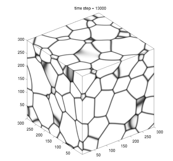
Figure 3: An example arrangement of crystals. The interfaces between pairs of crystals grow into each other according to motion by mean curvature. [This image is from Cenna/Wikimedia Commons/Public Domain [17].]

(5) $$\sum_{\alpha,\beta}\sigma_{\alpha\beta}\mathrm{Area}(\Gamma_{\alpha\beta})\,,$$

where $\displaystyle\Gamma_{\alpha\beta}$ is the interface between crystals $\displaystyle\alpha$ and $\displaystyle\beta$, and $\displaystyle\sigma_{\alpha\beta}$ is the surface-tension energy density between these crystals. Each $\displaystyle\sigma_{\alpha\beta}$ is different, based on physical considerations that involve the exact offset between the orientations of the lattices in each pair of crystals. When prepared and heated appropriately, the individual crystals decrease Eq. 5 by growing to consume their neighboring crystals. See [49, 43, 23] for further background information.

In the study of SBMs, one can use TV to express Eq. 2, but we find a more natural formulation in terms of surface-tension energy (a related notion). Specifically, we exploit the appearance of surface area in Eq. 5 to cast it as a TV problem. Mathematically, we model the metal as a region of space that is partitioned into $\displaystyle\hat{n}$ regions, corresponding to the crystals in the metal. Let $\displaystyle u^{\alpha}$ and $\displaystyle u^{\beta}$, respectively, denote the characteristic functions of the regions $\displaystyle\alpha$ and $\displaystyle\beta$. Therefore,

$$\mathrm{Area}_{\alpha\beta}=|u^{\alpha}|_{\text{TV}}+|u^{\beta}|_{\text{TV}}-|u^{\alpha}+u^{\beta}|_{\text{TV}}\,.$$

Each interface between two regions evolves according to mean-curvature flow. Consequently, the surface-tension flow is locally mean-curvature flow, except at the junction of three or more crystals [43, 23]. Because of this connection, one can use some of the ideas (such as phase-field and threshold-dynamics methods [23]) from TV minimization to perform surface-tension minimization. When using threshold dynamics, it is possible to do theoretical analysis in the form of Lyapunov functionals, $\displaystyle\Gamma$-convergence, and descent conditions [43].

3 An Equivalence Between SBM MLE and Discrete Surface Tension

We now present a mathematical result that connects SBM MLE and discrete surface tension.

Proposition 3.1.

Maximizing the likelihood of the parameters $\displaystyle g\in\{1,\hat{n}\}^{N}$ (i.e., node assignments) and $\displaystyle\omega$ (i.e., affinities) in the degree-corrected SBM (see Eq. 2) is equivalent to minimizing

(6) $$\sum_{\alpha,\beta}\left[W_{\alpha\beta}\mathrm{Cut}_{g,A}(\alpha,\beta)+e^{-W_{\alpha\beta}}\frac{\mathrm{vol}_{g,A}(\alpha)\,\mathrm{vol}_{g,A}(\beta)}{2m}\right]\,,$$

where $\displaystyle\mathrm{Cut}_{g,A}(\alpha,\beta)=\sum_{\begin{subarray}{c}g_{i}=\alpha\\ g_{j}=\beta\end{subarray}}A_{ij}$, the volume term is $\displaystyle\mathrm{vol}_{g,A}(\alpha)=\sum_{g_{i}=\alpha}k_{i}$, and $\displaystyle W_{\alpha\beta}=-\log\omega_{\alpha\beta}$ (so $\displaystyle W\in(-\infty,\infty]^{\hat{n}\times\hat{n}}$).

One immediately has the following well-posedness results. For a fixed $\displaystyle W$, the expression (6) has a solution, because the state space over which one is minimizing is of finite cardinality. Furthermore, for fixed $\displaystyle g$, one can find the optimal $\displaystyle W=W(g)$ in closed form by differentiating with respect to each component of $\displaystyle W$ and setting the result to $\displaystyle 0$ [46]. (We obtain a minimum of 6 because it is concave up.) Therefore, the full problem, in which we allow $\displaystyle W$ to vary, also has a solution, because there are a finite number of candidate pairs $\displaystyle(g,W(g))$. Uniqueness is not guaranteed, because one can permute the community labels (and the corresponding entries in $\displaystyle W$) to obtain another minimizer. Another source of non-uniqueness is the possibility of symmetries in the underlying graph, which allows any optimizer to be converted to another optimizer by permuting the node labels. Continuous dependence of the minimizer on $\displaystyle A$ is automatic, because the set of possible values for $\displaystyle A$ is discrete.

The analogy with continuum surface tension is as follows. Graph cuts are analogous to surface area: given a domain in $\displaystyle\mathbb{R}^{3}$, one can superimpose a fine grid on space and count the number of edges that cross the boundary to estimate its surface area. In the limit of an infinitely fine grid, this estimate converges to the surface area under appropriate conditions [13]. Similarly, graph volumes are analogous to continuum volumes. The quantities $\displaystyle W_{\alpha\beta}$ play the role of surface tensions $\displaystyle\sigma_{\alpha\beta}$, so the first set of terms is analogous to Eq. 5. One can view the second set of terms as a soft volume constraint. A constraint is “soft” if violating it adds a finite penalty on an objective function, so minimizers usually approximately satisfy the constraint. Volume-constrained versions of Eq. 5 have received a great deal of attention [49, 44].

We now prove Proposition 3.1.

Proof 3.2.

(Proposition 3.1)

In [65], it was shown that maximizing the log-likelihood of the parameters $\displaystyle g$ and $\displaystyle\omega$ for a particular version of the degree-corrected SBM amounts to maximizing Eq. 2. Let $\displaystyle\Pi(G,\hat{n})$ be the set of partitions of the nodes of a graph $\displaystyle G$ (associated with an adjacency matrix $\displaystyle A$) into at most $\displaystyle\hat{n}$ sets. Substituting $\displaystyle W_{\alpha\beta}=-\log\omega_{\alpha\beta}$ into Eq. 2 gives

$$\operatorname*{argmin}_{\begin{subarray}{c}W_{\alpha\beta}\in(-\infty,\infty]\\ g\in\Pi(G,\hat{n})\end{subarray}}\sum_{i,j}\left[A_{ij}W_{g_{i}g_{j}}+\frac{k_{i}k_{j}}{2m}e^{-W_{g_{i}g_{j}}}\right]\,.$$

Rearranging the summations gives

$$\operatorname*{argmin}_{\begin{subarray}{c}W_{\alpha\beta}\in(-\infty,\infty]\\ g\in\Pi(G,\hat{n})\end{subarray}}\left[\sum_{\alpha,\beta}\sum_{\begin{subarray}{c}g_{i}=\alpha\\ g_{j}=\beta\end{subarray}}A_{ij}W_{\alpha\beta}+\sum_{\alpha,\beta}\sum_{\begin{subarray}{c}g_{i}=\alpha\\ g_{j}=\beta\end{subarray}}\frac{k_{i}k_{j}}{2m}e^{-W_{\alpha\beta}}\right]\,,$$

where the inner sums are over all nodes $\displaystyle i$ and $\displaystyle j$ such that $\displaystyle g_{i}=\alpha$ and $\displaystyle g_{j}=\beta$. Rearranging again gives

$$\operatorname*{argmin}_{\begin{subarray}{c}W_{\alpha\beta}\in(-\infty,\infty]\\ g\in\Pi(G,\hat{n})\end{subarray}}\left[\sum_{\alpha,\beta}W_{\alpha\beta}\sum_{\begin{subarray}{c}g_{i}=\alpha\\ g_{j}=\beta\end{subarray}}A_{ij}+\sum_{\alpha,\beta}e^{-W_{\alpha\beta}}\sum_{\begin{subarray}{c}g_{i}=\alpha\\ g_{j}=\beta\end{subarray}}\frac{k_{i}k_{j}}{2m}\right]\,.$$

Using the definition of $\displaystyle\mathrm{Cut}_{g,A}$ in the first set of terms and summing over the $\displaystyle j$ index independently in the second set of terms gives

$$\operatorname*{argmin}_{\begin{subarray}{c}W_{\alpha\beta}\in(-\infty,\infty]\\ g\in\Pi(G,\hat{n})\end{subarray}}\left[\sum_{\alpha,\beta}W_{\alpha\beta}\mathrm{Cut}_{g,A}(\alpha,\beta)+\sum_{\alpha,\beta}e^{-W_{\alpha\beta}}\sum_{g_{i}=\alpha}\frac{k_{i}}{2m}\mathrm{vol}_{g,A}(\beta)\right]\,.$$

Finally, we sum over the $\displaystyle i$ index in the second set of terms to obtain

(7) $$\operatorname*{argmin}_{\begin{subarray}{c}W_{\alpha\beta}\in(-\infty,\infty]\\ g\in\Pi(G,\hat{n})\end{subarray}}\sum_{\alpha,\beta}\left[W_{\alpha\beta}\mathrm{Cut}_{g,A}(\alpha,\beta)+e^{-W_{\alpha\beta}}\frac{\mathrm{vol}_{g,A}(\alpha)\,\mathrm{vol}_{g,A}(\beta)}{2m}\right]\,.$$

One difference between Eq. 6 and Eq. 5 is that in Eq. 6, one performs optimization over the $\displaystyle W_{\alpha\beta}$, whereas in Eq. 5 (i.e., in a continuum), one ordinarily treats the surface-tension densities as fixed by the choice of material that one is modeling. Another difference is that the surface-tension coefficients in the graph setting can be any element of $\displaystyle(-\infty,\infty]$, subject only to the symmetry condition $\displaystyle W_{\alpha\beta}=W_{\beta\alpha}$ (see Section 2). By contrast, for a continuum, one needs further restrictions to ensure well-posedness. Esedoglu and Otto [23] proved the following sufficient conditions for well-posedness:

• $\displaystyle\sigma_{\alpha\beta}\geq 0$  ,

• $\displaystyle\sigma_{\alpha,\alpha}=0$  ,

• $\displaystyle\sigma_{\alpha\gamma}+\sigma_{\gamma\beta}\geq\sigma_{\alpha\beta}$ .

In a graph setting, one can use a straightforward change of variables, $\displaystyle W_{\alpha\beta}\to W_{\alpha\beta}-\frac{1}{2}W_{\alpha\alpha}-W_{\beta\beta}$, to make $\displaystyle W$ satisfy requirement (2). In general, however, at least one of requirements (1) and (3) is not necessarily satisfied for a graph. Requirement (1) is false whenever some component of $\displaystyle W$ is negative; this occurs exactly when $\displaystyle\omega$ has a component that is larger than $\displaystyle 1$. In the continuum, requirement (3) has the interpretation of preventing “wetting,” where one phase can spontaneously appear between two others. In the graph case, such a restriction is unnecessary, because the number of points is fixed and finite, with no possibility of inserting points of another phase between two nodes.

The analogy of Eq. 6 with continuum surface tension is simplest for the case of assortative communities, although it is also relevant for other types of block structure. For disassortative blocks, rather than an energy cost from surface area, particles in one phase can achieve a lower energy by interacting with particles in a different phase. This leads to solutions that maximize surface area, and the evolutions that we will consider in Section 4 then involve backward diffusion. In the continuum case, this is ill-posed; however, a graph does not include arbitrarily small length scales, so ill-posedness does not cause a problem. Backward diffusion on graphs also appeared recently in [100] in the context of image processing, and it would be interesting to see if their techniques would be insightful in our context. For core–periphery structure, one phase has an energy penalty from interacting with itself but lowers its energy by interacting with the other phase. The other phase, however, prefers to interact with itself. As far as we are aware, such structures have not been studied previously in the literature on surface-tension models of crystal growth. For more complicated block structures, it is concomitantly more complicated to interpret the analogy with continuum surface tension. In a sense, one should view the SBM in Eq. 6 as a generalization of discrete surface tension, rather than as an analog. In the present paper, we emphasize applications to assortative community structure.

4 Mean-Curvature Flow (MCF), $\displaystyle\Gamma$-Convergence, and Threshold Dynamics

We now outline three algorithmic approaches that illustrate how one can use tools from surface-tension theory to solve SBM MLE problems. Our three algorithms are graph versions of mean-curvature flow (MCF), Allen–Cahn (AC) evolution, and Merriman–Bence–Osher (MBO) dynamics. In Section 5, we will conduct several numerical experiments to demonstrate that these algorithms can effectively solve Eq. 2. We expect the performance of these algorithms to be good relative to other algorithms for SBM MLE, although a full evaluation of this claim is beyond the scope of our paper. We have posted our code at github.com/zboyd2/SBM-surface-tension. In the next three subsections, we describe how we infer $\displaystyle g$ when $\displaystyle\omega$ is fixed and finite. We then describe how to jointly infer $\displaystyle\omega$ and $\displaystyle g$.

4.1 Mean-Curvature Flow

Surface-tension dynamics are governed by mean-curvature flow except at junctions. Intuitively, each point on a surface moves in the direction normal to the surface at a speed given by the mean curvature at that point. In the two-phase case, such dynamics have been well-studied, and there exist notions of viscosity solutions and regularity theory [56]. In the multiphase case, the situation is much more complicated, especially because of the topological changes that can occur and the issue of defining the behavior at the junction of three or more phases. In two-phase surface-tension dynamics, it was shown in [14] that one can approximate the flow by solving a discrete-time minimizing-movements problem. Let $\displaystyle C_{n}$ be one of the two regions at time $\displaystyle n\,dt$, where $\displaystyle dt$ is the time step. To update $\displaystyle C_{n}$, one uses

(8) $$C_{n+1}=\operatorname*{argmin}_{C}\left[\mathrm{SurfaceArea}(C)+\frac{1}{dt}\int_{C_{n}\Delta C}\hat{\rho}(p,C_{n})\mathrm{d}p\right],$$

where

$$\hat{\rho}(p,C_{n})=\inf_{x\in\partial C_{n}}\|x-p\|\,,$$

the operation $\displaystyle\Delta$ denotes the symmetric difference, and $\displaystyle\partial$ is the topological boundary operator. The idea behind this approach is, at each time step, to shorten the curve as much as possible without straying too far from the curve location at the previous time step.

In the setting of graphs, a similar approach was developed in [95], where the mean-curvature flow was given by

(9) $$C_{n+1}=\operatorname*{argmin}\left[\mathrm{Cut}_{g,A}(C,C^{c})+\frac{1}{dt}\sum_{i\in C_{n}\Delta C}\rho(i,\partial(C_{n}))\right]\,,$$

the operation $\displaystyle\Delta$ is again the symmetric difference, and $\displaystyle\rho(i,\partial(C_{n}))$ is the shortest-path distance from node $\displaystyle i$ to the boundary of $\displaystyle C_{n}$. In this context, the boundary of a set of nodes is the set of nodes in $\displaystyle C_{n}$ with at least one neighbor in $\displaystyle C_{n}^{c}$ along with the nodes in $\displaystyle C_{n}^{c}$ that have at least one neighbor in $\displaystyle C_{n}$. We use the term boundary node for any node that lies on the boundary. In the limit of small $\displaystyle dt$, Eq. 9 may still evolve, as opposed to the MBO scheme (which we use later), which becomes “stuck” when the time step is too small. Such evolution can still occur, because the penalty (associated with moving any node in $\displaystyle\partial(C_{n})$) induced by the second set of terms in Eq. 9 is $\displaystyle 0$, regardless of the value of $\displaystyle dt$. Conveniently, this implies for sufficiently small $\displaystyle dt$ that the only acceptable moves at each time step are ones that are allowed to change only the boundary nodes themselves. This makes it possible to drastically reduce the search space when solving Eq. 9.

Because careful studies in the spirit of [95] are not yet available for multi-way graph partitioning, we resort to a heuristic approach based on what is known for bipartitioning. Specifically, we are motivated by the situation in which time steps are sufficiently small that only boundary nodes can change their community assignment. Ideally, we wish to compute an optimal reassignment of all boundary nodes jointly to minimize Eq. 6. To save computation time and facilitate implementation, we instead decouple the computations in the following manner. During a single time step, for each boundary node, we compute an optimal assignment of that node, assuming that all other nodes keep their assignment from the beginning of the time step. After this (but before the end of the time step), we assign each boundary node to its community, as computed previously in the time step. Because most nodes are boundary nodes in our SBM-generated graphs, we find it both more efficient and easier to consider reassigning all nodes in each time step, rather than maintaining and referencing a separate data structure to track the boundary. For other networks and initialization techniques, such as in networks that arise from nearest-neighbor graphs with initialization from spectral clustering, it may be more efficient to loop over only the boundary nodes. (This idea aligns particularly with the spirit of mean-curvature flow.) In Algorithm 1, we give pseudocode for this graph MCF procedure.

Input $\displaystyle A$, $\displaystyle W$, $\displaystyle\hat{n}$ .

Initialize $\displaystyle g$ so that nodes are assigned to communities uniformly at random.

Let $\displaystyle\mathrm{eW}=e^{-W}$  be the entry-wise exponential of $\displaystyle W$ .

while not converged do

     Let $\displaystyle U_{i\alpha}=\delta_{g_{i}\alpha}$ for each $\displaystyle i,\alpha$, where $\displaystyle\delta$ is the Kronecker delta.

     Let $\displaystyle X=AU$ .  // Counts the number of neighbors that each node has in each community

     Let $\displaystyle\mathrm{vol}_{g,A}=(k^{T}U)$ .

     for $\displaystyle a^{\prime}=1$ to $\displaystyle\hat{n}$ do

         Let $\displaystyle I_{a^{\prime}}$ be the set of nodes that are currently assigned to community. $\displaystyle a^{\prime}$ .

         for a=1 to $\displaystyle\hat{n}$ do

              Let $\displaystyle I$ be the indices $\displaystyle 1,\ldots,\hat{n}$ aside from $\displaystyle a$ and $\displaystyle a^{\prime}$ .

              Let $\displaystyle\mathrm{Delta}(I_{a^{\prime}},a)$ be given by the following formula:

$$\displaystyle\mathrm{Delta}(I_{a^{\prime}},a) \displaystyle=2X(I_{a^{\prime}},I)W(I,a)$$

$$\displaystyle-2X(I_{a^{\prime}},I)W(I,a^{\prime})$$

$$\displaystyle+2X(I_{a^{\prime}},a)W(a,a)$$

$$\displaystyle-2X(I_{a^{\prime}},a)W(a,a^{\prime})+2X(I_{a^{\prime}},a^{\prime})W(a,a^{\prime})$$

$$\displaystyle-2X(I_{a^{\prime}},a^{\prime})W(a^{\prime},a^{\prime})$$

$$\displaystyle+\frac{1}{2m}\left(2k(I_{a^{\prime}})\mathrm{vol}_{g,A}(\mathrm{eW}(:,a)-\mathrm{eW}(:,a^{\prime}))\right.$$

$$\displaystyle+\left.k(I_{a^{\prime}})^{2}(\mathrm{eW}(a,a)+\mathrm{eW}(a^{\prime},a^{\prime})-2\mathrm{eW}(a,a^{\prime}))\right).$$

         end for

     end for

     for $\displaystyle i=1$ to $\displaystyle N$ do

         $\displaystyle g_{i}=\operatorname*{argmin}(\mathrm{Delta(i,:)})$ .  // [Choose uniformly at random in case of a tie.]

     end for

end while

Output $\displaystyle g$ .

Algorithm 1 Modified graph mean-curvature flow (MCF) for SBM MLE Eq. 2.

4.2 Allen–Cahn (AC) Evolution

Another approach for studying MCF is approximation by a Ginzburg–Landau (GL) functional. This approach is popular due to its simple implementation and the existence of unconditionally-stable numerical methods [7].

In the two-phase case, the GL functional is

(10) $$\int_{\Omega}\left[\epsilon\left|\operatorname{\nabla}u\right|^{2}+\frac{1}{2\epsilon}u^{2}(1-u)^{2}\right]\mathrm{d}x\,,$$

where $\displaystyle u:\Omega\subset\mathbb{R}^{N}\to\mathbb{R}$ is a smooth function and $\displaystyle\epsilon$ is a small parameter.

The $\displaystyle L^{2}$ gradient descent of the GL functional is

$$u_{t}=\epsilon\Delta u-\frac{1}{2\epsilon}\frac{\mathrm{d}}{\mathrm{d}u}\left[u^{2}(1-u)^{2}\right]\,,$$

which is the Allen–Cahn (AC) equation. The minimizers of the GL energy are predominantly (piecewise) constant, with $\displaystyle O(\epsilon)$-width transition layers between the constant regions. One can show that the GL energy $\displaystyle\Gamma$-converges to the TV energy as $\displaystyle\epsilon\to 0$, assuming that $\displaystyle\int_{\Omega}u\,\mathrm{d}x=\operatorname{const}$ [61]. Consequently, if $\displaystyle u_{\epsilon}$ is a minimizer of the constrained GL energy with parameter $\displaystyle\epsilon$ and the minimizers converge in $\displaystyle L^{1}$ as $\displaystyle\epsilon\to 0$, then the accumulation point is a minimizer of the TV energy.

In the setting of graphs, the first use of AC schemes for TV minimization was in [7]. One can invoke the combinatorial graph Laplacian $\displaystyle L=\mathrm{diag}(k)-A$ to obtain a graph GL functional

(11) $$U^{T}LU+\frac{1}{\epsilon}U^{2}(1-U^{2})\,,$$

where $\displaystyle U$ is a function on the graph nodes (so it is an $\displaystyle N$-element vector) and $\displaystyle\epsilon$ is again a positive number. Expression (11) $\displaystyle\Gamma$-converges to graph TV [94].

In the multiphase case, we represent the community assignments $\displaystyle g$ in terms of an $\displaystyle N\times\hat{n}$ matrix whose $\displaystyle i,\alpha$ entry is $\displaystyle\delta_{g_{i}\alpha}$, where $\displaystyle\delta$ is the Kroneker delta. Instead of a double-well potential, we use a multi-well potential on $\displaystyle\mathbb{R}^{N\times\hat{n}}$ whose value is minimized by arguments with exactly one nonzero entry in each row. For example, Garcia-Cardona et al. [31] proposed the following potential:

$$T(U)=\sum_{i=1}^{N}\left(\prod_{\alpha=1}^{\hat{n}}\frac{1}{4}\left\|U_{i}-e_{k}\right\|^{2}_{\ell^{1}}\right)\,,$$

where $\displaystyle U_{i}$ is the $\displaystyle i$th row of the $\displaystyle N\times\hat{n}$ matrix $\displaystyle U$ and $\displaystyle e_{k}$ is an $\displaystyle\hat{n}$-element vector that is equal to $\displaystyle 0$ except for a $\displaystyle 1$ in the $\displaystyle k$th entry.

For the particular case of surface-tension dynamics, we proceed as follows. Additionally, we assume in this subsection and the next that we have already eliminated the diagonal of $\displaystyle W$ (see Appendix A).

Given community assignments (and hence a partition of a network), if $\displaystyle U$ is the corresponding $\displaystyle N\times\hat{n}$ matrix, one can show that $\displaystyle W.*(U^{T}LU)=-W.*(U^{T}AU)$, where $\displaystyle.*$ is the entry-wise product. Therefore, an appropriate GL functional for our problem is

(12) $$\sum_{\alpha,\beta}\left[-W_{\alpha\beta}U_{\alpha}^{T}LU_{\beta}+\frac{\mathrm{vol}_{g,A}(\alpha)\,\,e^{-W}_{\alpha\beta}\,\,\mathrm{vol}_{g,A}(\beta)}{2m}\right]+\sum_{\alpha}W_{\alpha\alpha}\mathrm{vol}_{g,A}(\alpha)+\frac{1}{2\epsilon}T(U)\,.$$

Because $\displaystyle k^{T}U$ gives the vector of volumes, one can rewrite Eq. 12 as

(13) $$\sum_{\alpha,\beta}\left[-W_{\alpha\beta}U_{\alpha}^{T}LU_{\beta}+\frac{k^{T}U_{\alpha}e^{-W}_{\alpha\beta}U_{\beta}^{T}k}{2m}\right]+\sum_{\alpha}W_{\alpha\alpha}\mathrm{vol}_{g,A}(\alpha)+\frac{1}{2\epsilon}T(U)\,,$$

where $\displaystyle e^{-W}$ is the entry-wise exponential.

As in a continuum setting, one can prove $\displaystyle\Gamma$-convergence.

Theorem 4.1.

Let $\displaystyle W\in\mathbb{R}^{\hat{n}\times\hat{n}}$. The functionals in Eq. 13 $\displaystyle\Gamma$-converge (as functions on $\displaystyle\mathbb{R}^{N\times\hat{n}}$) to Eq. 6 as $\displaystyle\epsilon\to 0$.

See Appendix B for a proof. As far as we are aware, this is the first $\displaystyle\Gamma$-convergence result for a multiphase graph energy on arbitrary graphs. However, see [71, 92, 90] for $\displaystyle\Gamma$-convergence applied to consistency of multiphase geometric graph energies.

The resulting AC equation is

(14) $$U_{t}=LUW-\frac{1}{2m}kk^{T}Ue^{-W}-k.*\operatorname{diag}(W)-\frac{1}{\epsilon}T^{\prime}(U)\,.$$

See Appendix C for further details on the numerical solution of Eq. 14.

4.3 MBO Iteration

Input the initial domain.

Initialize $\displaystyle u$ as the characteristic function of the initial domain.

for $\displaystyle i=1,\ldots$ do

     $\displaystyle u^{i+1/2}$ is the solution at time $\displaystyle dt$ of $\displaystyle u_{t}=\Delta u$ with initial condition $\displaystyle u^{i}$ .

     $\displaystyle u^{i+1}=\lfloor u^{i+1/2}+0.5\rfloor$ , where $\displaystyle\lfloor\cdot\rfloor$ is the floor function.

end for

Output the set of points for which $\displaystyle u=1$ .

Algorithm 2 A two-phase, continuum MBO scheme.

In [60], Merriman, Bence, and Osher showed that continuum MCF is well-approximated by the simple iteration in Algorithm 2. In a rectangular domain, the iteration is extremely efficient, as one can use a fast Fourier transform when solving the heat equation. Esedoglu and Otto [23] developed a generalized version of the MBO scheme (see  Algorithm 3) for computing the evolution of multiphase systems that are modeled by Eq. 5.

Input the initial state of the domain.

Initialize $\displaystyle u_{1},\ldots,u_{\hat{n}}$ as the characteristic functions of the initial domains.

for $\displaystyle i=1,\ldots$ do

     for $\displaystyle\alpha=1,\ldots,\hat{n}$ do

         $\displaystyle u^{i+1/2}_{\alpha}$ is the solution at time $\displaystyle dt$ to $\displaystyle u_{\alpha,t}=\Delta u_{\alpha}$ with initial condition $\displaystyle u^{i}_{\alpha}$ .

     end for

     for each point $\displaystyle x$ do

         $\displaystyle\hat{\alpha}=\operatorname*{argmin}_{\alpha}\sum_{\beta}\sigma_{\alpha\beta}u_{\beta}(x)\,.$  // [Choose uniformly at random in case of a tie]

         $\displaystyle u_{\hat{\alpha}}(x)=1$ and $\displaystyle u_{\beta}(x)=0$ if $\displaystyle\beta\neq\hat{\alpha}$ .

     end for

end for

Output $\displaystyle u$ .

Algorithm 3 A multiphase, continuum MBO scheme.

One can apply the MBO idea to community detection in networks by replacing the continuum Laplacian with the (negative) combinatorial graph Laplacian, replacing $\displaystyle\sigma$ with $\displaystyle W$, changing $\displaystyle u$ to $\displaystyle U$, and adding appropriate forcing terms for the gradient descent of the volume-balance terms. See Appendix C for additional implementation details.

4.4 Learning $\displaystyle\omega$

The MCF, AC, and MBO algorithms are able to produce a good partition of a network, given $\displaystyle W$, but they do not include a way to find $\displaystyle W$. A simple way to address this issue is to use an expectation-maximization (EM) algorithm, in which one alternates between solving for $\displaystyle g$ with fixed $\displaystyle W$ (using MCF, AC, or MBO) and solving for $\displaystyle W$ with fixed $\displaystyle g$. Given $\displaystyle g$, one can find a closed-form expression for the optimal $\displaystyle W$ by differentiating Eq. 6 with respect to any component of $\displaystyle W$ and setting the result to $\displaystyle 0$ [46].

One must be careful, however, because the optimal $\displaystyle W_{\alpha\beta}$ is infinite when $\displaystyle\mathrm{Cut}_{g,A}(\alpha,\beta)=0$. This is problematic, because once one of the entries in $\displaystyle W$ is infinite, it prevents $\displaystyle g$ in subsequent iterations from taking any nonzero value of $\displaystyle\mathrm{Cut}_{g,A}(\alpha,\beta)$; this gives bad results in our test examples. (See Section 5 for a discussion of these examples.) We address this issue by modifying the EM algorithm to reset all infinite values of $\displaystyle W$ to $\displaystyle 1.1\times W_{\text{max}}$, where $\displaystyle W_{\text{max}}$ is the largest non-infinite element of $\displaystyle W$ and $\displaystyle 1.1$ is a (hand-tuned) parameter that allows moderate growth in $\displaystyle W$.

We also need to address another practical issue for an EM approach to work. Specifically, the algorithm that we have described thus far in this section often finds bad local minima in which communities are merged erroneously or a single community is split inappropriately.

To overcome this issue, we implement a wrapper function (see  Algorithm 4) that checks each community that is returned by MCF, AC, or MBO for further possible splitting or merging with other communities. Whenever we call MCF, AC, or MBO on a subgraph, we use the values of $\displaystyle k$ and $\displaystyle m$ for the whole graph rather than those for a subgraph. A similar idea was used in [64, 42] for their recursive partitioning procedures.

There is also a danger of overfitting by setting $\displaystyle\hat{n}=N$, which gives a likelihood of $\displaystyle 1$ in Eq. 2. The proper selection of $\displaystyle\hat{n}$ is a complicated problem, both algorithmically and theoretically [69, 82]. For our tests, we were very successful by using a simple heuristic approach. (Our framework is also compatible with more sophisticated methods for selecting $\displaystyle\hat{n}$.) For each data set, we supply an expected value of $\displaystyle\hat{n}$ for that data set, and we then add a quadratic penalty to the objective-function value whenever $\displaystyle\hat{n}$ differs from its expected value. This helps curtail overfitting, while still allowing our algorithms to perform merges and splits to escape bad local minima. Notably, this penalty does not alter the MCF, AC, or MBO procedures; instead, it is part of Algorithm 4.

Input $\displaystyle A$, $\displaystyle\hat{n}_{\text{expected}}$ .

Place all nodes in the same community and add this community to a queue.

while the queue is not empty do

     Save $\displaystyle g_{\text{old}}=g$ and $\displaystyle W_{\text{old}}=W$ .

     Save the current objective-function value as $\displaystyle Q_{\text{old}}$ .

     Partition the next community (as an induced subgraph, as we include all associated edges) in the queue into $\displaystyle\min\{\hat{n}_{\text{expected}},\sqrt{N}\}$ communities using MCF, AC, or MBO with $\displaystyle w_{\alpha\beta}=\begin{cases}1\,,&\alpha=\beta\,,\\ 0.1\,,&\alpha\neq\beta\,.\end{cases}\,.$

     while it is possible to improve the objective-function value by merging two partition elements do

         Perform the merge that most improves the objective function.

     end while

     if the objective-function value is larger than $\displaystyle Q_{\text{old}}$ then

         Add any newly created communities to the queue.

     else

         Set $\displaystyle g=g_{\text{old}}$ and $\displaystyle W=W_{\text{old}}$ .

         Remove the current community from the queue.

     end if

end while

Output $\displaystyle g$, $\displaystyle W$ .

Algorithm 4 Our splitting–merging wrapper for escaping from bad local minima. In this algorithm, $\displaystyle Q$ is the objective function from Eq. 6 multiplied by $\displaystyle[1+0.1\left(\hat{n}-\hat{n}_{\text{expected}}\right)^{2}]$, where we chose the value $\displaystyle 0.1$ based on hand-tuning.

5 Empirical Results

We now discuss our results from several numerical experiments to (1) confirm that our algorithms can successfully recover $\displaystyle g$ and $\displaystyle\omega$ from networks that we generate using SBMs and (2) explore their applicability to real-world networks. In our experiments, we use three different families of SBMs, three Facebook networks (whose community structure is partly understood [88, 89]), and an example related to hyperspectral video segmentation. Because of the random initialization in our approach, we perform three trials on each of the networks for each algorithm, and we report the best result in each case. For comparison, we also report the results of a Kernighan–Lin (KL) algorithm, which was reported in [46] to be effective. We summarize our results in Table 1, and we highlight that we consistently recover the underlying structure in the synthetic examples. For the real networks, we compare our results with a reference partition based on metadata that is thought to be correlated with the community structure. We find that the MCF scheme performs the best among our three schemes on these networks, and it finds partitions with a larger likelihood than the reference partition. We implement our methods in Matlab, so one should interpret computation times in Table 2 as indicative that the run time is reasonable for networks with millions of edges. Given a careful implementation in a compiled language, it is possible to study even larger networks. For an example of code for a similar problem that was solved by an MBO scheme at large scale (including a weighted graph with almost $\displaystyle 14$ million nodes and $\displaystyle 1.8\times 10^{14}$ edges), see [57].

We briefly describe the three families of SBM-related networks that we use in our numerical experiments.

• Planted partition (PP) is a 16,000-node graph that consists of $\displaystyle 10$ equal-size communities. It is produced by the method that was described in [46]. It builds a degree-corrected SBM with a truncated power-law degree distribution with exponent $\displaystyle 2$. The parameter $\displaystyle\lambda$ from Equation (27) in [46] is $\displaystyle 0.001$, indicating a fairly clear separation between communities.

• Lancichinetti–Fortunato–Radicchi (LFR) is a standard benchmark SBM network [52]. We construct 1000-node LFR graphs with a power-law degree distribution (with exponent $\displaystyle 2$), mean degree $\displaystyle 20$, maximum degree $\displaystyle 50$, power-law-distributed community sizes (with exponent $\displaystyle 1$), community sizes between $\displaystyle 10$ and $\displaystyle 50$ nodes, and mixing parameter $\displaystyle 0.1$.

• Multiscale SBM (MS). To construct such a graph, we take a sequence of disjoint components; in order, these are a $\displaystyle 10$-clique, a $\displaystyle 20$-clique, and a sequence of Erdős–Rényi (ER) graphs (drawn from the $\displaystyle G(n,p)$ model with $\displaystyle n$ nodes and $\displaystyle np=20$) of sizes $\displaystyle 40$, $\displaystyle 80$, $\displaystyle 160$, …, $\displaystyle 5120$. Each of these graphs has a total of $\displaystyle 10,230$ nodes. In each such graph, we connect the components to each other by adding a single edge, from nodes chosen uniformly at random, between each consecutive clique or ER graph. This construction tests whether an algorithm can find communities of widely varying sizes in the same graph [26, 2].

The hyperspectral video is a recording of a gas plume as it was released at the Dugway Proving Ground [32, 55, 59]. A hyperspectral video is different from an RGB video, in that each pixel in the former encodes the intensity of light at a large number (e.g., $\displaystyle 129$, in this case) of different wavelengths rather than at only $\displaystyle 3$, with each channel corresponding to a wavelength. We consider the classification problem of identifying pixels that include similar materials (such as dirt, road, grass, and so on). This problem is difficult because of the diffuse nature of the gas, which leads to a faint signal that spreads out among many wavelengths and with boundaries that are difficult to determine. We construct a graph representation of this video using “nonlocal means,” as described in [15]. Specifically, we use the following construction. For each pixel $\displaystyle p$ and in each of $\displaystyle 7$ frames, we construct a vector $\displaystyle v_{p}$ by concatenating the data in a $\displaystyle 3\times 3$ window that is centered at $\displaystyle p$. We then use a weighted cosine similarity measure (which is a common choice for hyperspectral imaging applications) on these $\displaystyle(3\times 3\times 129)$-component vectors, where we give the most weight to the components from the center of the window. Finally, using the VLFeat software package [96], we build an unweighted 10-nearest-neighbor graph using the similarity measure and a $\displaystyle k$-dimensional tree (with $\displaystyle k=10$) [6]. We see from Fig. 4 that partitions with small values of Eq. 6 correspond to meaningful segmentations of the image.

		PP	LFR	MS	Caltech	Princeton	Penn. St.	Plume
	Nodes	16,000	1,000	10,230	762	6,575	41,536	284,481
	Edges	$\displaystyle 2.9\times 10^{5}$	$\displaystyle 9.8\times 10^{3}$	$\displaystyle 1.0\times 10^{5}$	$\displaystyle 16,651$	$\displaystyle 293,307$	$\displaystyle 1,362,220$	$\displaystyle 2,723,840$
	Communities	10	40	10	8	4	8	5
Score	MCF	0	0	0	$\displaystyle-0.16$	$\displaystyle-0.02$	$\displaystyle-0.56$	$\displaystyle-1.41$
	AC	0	0	0	0.21	0.58	$\displaystyle-0.04$	$\displaystyle-1.23$
	MBO	0	0	0	0.53	1.12	0.40	$\displaystyle-1.21$
	KL	0.28	0.03	0.04	$\displaystyle-0.16$	0.11	$\displaystyle-0.55$	$\displaystyle-1.38$
	Reference	0	0	0	0	0	0	0

Table 1: Results of several tests on several synthetic and empirical networks. We use three surface-tension-based methods (mean-curvature flow, Allen–Cahn, and Merriman–Bence–Osher) and the Kernighan–Lin algorithm from [46] to partition three synthetic networks (Planted Partition, LFR, and Multiscale SBM) and the largest connected components of three empirical networks (Caltech36, Princeton12, and Penn94) from the Facebook100 data set [89]. The score is the recovered surface-tension energy Eq. 6 minus the corresponding energy of a reference partition, divided by the absolute value of the energy of the reference partition. Smaller values indicate better performance, and $\displaystyle 0$ corresponds to a partition that is of comparable quality as the reference partition. For the synthetic networks, we use the planted (and hence ground-truth) community structure as the reference partition. For the Facebook networks, we use metadata that is positively correlated with community structure (namely, House affiliation for Caltech and graduation year for the other two networks). For the plume video, our reference partition is to assign all nodes to the same community, because no pixel-level metadata is associated with the images. The edge counts on the synthetic networks constitute an order-of-magnitude approximation, because the exact number differs across the three instantiations of these models. (This table gives the best result among three tests for each example; for the random-graph models, each such example is a different graph from the same model.)

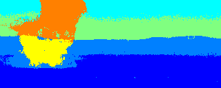
Figure 4: Segmentation of a hyperspectral video using graph MCF. The gas plume is clearly represented in the yellow and orange pixels. The two blue communities on the bottom are the ground, and the other two communities are the sky. This image is frame 3 of 7. (It is best to view this plot in color.)

	PP	LFR	MS	Caltech	Princeton	Penn. State	Plume
MCF	5.36	17.71	3.47	1.39	1.46	38.91	77.91
AC	5.37	26.27	7.28	8.84	480.4	3853	268.7
MBO	4.27	11.05	1.73	0.67	7.43	382.31	270.0
KL	16,566	176	5,117	20	662	95,603	980,520

Table 2: Median computation times (in seconds) for our example networks.

In Table 3, we show an example of a $\displaystyle W$ matrix that we obtain from an MS network to illustrate that we recover different surface tensions between different pairs of communities.

0	5.22	$\displaystyle\infty$	$\displaystyle\infty$	$\displaystyle\infty$	$\displaystyle\infty$	$\displaystyle\infty$	$\displaystyle\infty$	$\displaystyle\infty$	$\displaystyle\infty$
5.22	0	6.1817	$\displaystyle\infty$	$\displaystyle\infty$	$\displaystyle\infty$	$\displaystyle\infty$	$\displaystyle\infty$	$\displaystyle\infty$	$\displaystyle\infty$
$\displaystyle\infty$	6.1817	0	6.8471	$\displaystyle\infty$	$\displaystyle\infty$	$\displaystyle\infty$	$\displaystyle\infty$	$\displaystyle\infty$	$\displaystyle\infty$
$\displaystyle\infty$	$\displaystyle\infty$	6.8471	0	7.6316	$\displaystyle\infty$	$\displaystyle\infty$	$\displaystyle\infty$	$\displaystyle\infty$	$\displaystyle\infty$
$\displaystyle\infty$	$\displaystyle\infty$	$\displaystyle\infty$	7.6316	0	8.362	$\displaystyle\infty$	$\displaystyle\infty$	$\displaystyle\infty$	$\displaystyle\infty$
$\displaystyle\infty$	$\displaystyle\infty$	$\displaystyle\infty$	$\displaystyle\infty$	8.362	0	9.0869	$\displaystyle\infty$	$\displaystyle\infty$	$\displaystyle\infty$
$\displaystyle\infty$	$\displaystyle\infty$	$\displaystyle\infty$	$\displaystyle\infty$	$\displaystyle\infty$	9.0869	0	9.7926	$\displaystyle\infty$	$\displaystyle\infty$
$\displaystyle\infty$	$\displaystyle\infty$	$\displaystyle\infty$	$\displaystyle\infty$	$\displaystyle\infty$	$\displaystyle\infty$	9.7926	0	10.4911	$\displaystyle\infty$
$\displaystyle\infty$	$\displaystyle\infty$	$\displaystyle\infty$	$\displaystyle\infty$	$\displaystyle\infty$	$\displaystyle\infty$	$\displaystyle\infty$	10.4911	0	11.1869
$\displaystyle\infty$	$\displaystyle\infty$	$\displaystyle\infty$	$\displaystyle\infty$	$\displaystyle\infty$	$\displaystyle\infty$	$\displaystyle\infty$	$\displaystyle\infty$	11.1869	0

Table 3: Optimal surface tensions for the MS SBM example. (The entries are heterogeneous, so there are different surface tensions between different pairs of communities.) The infinite entries correspond to sets with no observed edge between them.

6 Conclusions and Discussion

We have shown that a particular stochastic block model (SBM) maximum-likelihood estimation (MLE) problem is equivalent to a discrete version of a well-known surface-tension problem. This equivalence, which associates graph cuts to surface areas and SBM parameters to physical surface tensions, gives new geometric and physical interpretations to SBM MLE problems, which are traditionally viewed from a statistical perspective. We used the new connection to adapt three well-known surface-tension-minimization algorithms to community detection in graphs. Our subsequent computations suggest that the resulting algorithms are able to successfully find underlying community structure in SBM-related graphs. When applied to graphs that are constructed from empirical data, our mean-curvature-flow (MCF) method performs very well, but the other two methods face some issues (which will be interesting to explore in future studies). We also proved a $\displaystyle\Gamma$-convergence result that gives theoretical justification for our algorithms.

Although our paper has focused on a specific form of an SBM and an associated MLE problem, our techniques should also be insightful for other studies of SBMs and their applications. One straightforward adaption is to consider SBMs without degree correction, although that is more interesting for theoretical work than for applications. Additionally, it seems promising to incorporate priors on the values of $\displaystyle g$ and $\displaystyle\omega$ as regularizers in the surface-tension energy (perhaps in a way that is similar to the procedure in [9]). Another viable extension is to incorporate a small amount of supervision into the community-inference process using techniques (such as quadratic fidelity terms) from image processing. A similar idea was used for modularity maximization in [42] and was tested further in [12].

Introducing supervision helps alleviate severe nonconvexity by penalizing local minima that are inconsistent with the (ideally) ground-truth classifications from which one draws the supervision. It is also important to generalize our approach to more complicated types of networks, such as multilayer [50] and temporal networks [40], and to incorporate metadata [67] into our inference methodology. For example, given our successful results on the hyperspectral video, it may be particularly interesting to use temporal network clustering to analyze time-dependent communities in the video.

Approaches such as inference using SBMs and modularity maximization are also related to other approaches for community detection, and the results in the present paper may help further illuminate those connections. These include recent work that relates SBMs to local methods for community detection that are based on personalized PageRank [51] and very recent work that established new connections between modularity maximization and several other approaches [97]. We expect that further mapping of the relations between the diverse available perspectives for community detection (and other problems in network clustering) will yield many new insights for network theory, algorithms, and applications.

Appendix A Eliminating the Diagonal Elements of $\displaystyle W$

It is difficult to interpret the parameters $\displaystyle W_{\alpha\alpha}$ in the context of Eq. 6 and our surface-tension analogy, because they correspond to “internal” surface tensions of a single crystal. In this appendix, we use a change of variables to eliminate these diagonal terms and replace them with additional volume terms, which are much easier to interpret.

We begin with the identity

(15) $$\displaystyle\sum_{\alpha,\beta}W_{\alpha\beta}\mathrm{Cut}_{g,A}(\alpha,\beta)=\sum_{\alpha}\sum_{\beta\neq\alpha}W_{\alpha\beta}\mathrm{Cut}_{g,A}(\alpha,\beta)+\sum_{\alpha}W_{\alpha\alpha}\mathrm{Cut}_{g,A}(\alpha,\alpha)\,,$$

and we compute

$$\displaystyle\sum_{\alpha}W_{\alpha\alpha}\mathrm{Cut}_{g,A}(\alpha,\alpha) \displaystyle=\sum_{\alpha}W_{\alpha,\alpha}\sum_{g_{i}=\alpha,g_{j}=\alpha}w_{ij}$$

$$\displaystyle=\sum_{\alpha}W_{\alpha,\alpha}\left(\sum_{g_{i}=\alpha,j=1,\dots,N}w_{ij}-\sum_{g_{i}=\alpha,g_{j}\neq\alpha}w_{ij}\right)$$

$$\displaystyle=\sum_{\alpha}W_{\alpha,\alpha}\left(\sum_{g_{i}=\alpha}k_{i}-\sum_{\beta\neq\alpha,g_{i}=\alpha,g_{j}=\beta}w_{ij}\right)$$

(16) $$\displaystyle=\sum_{\alpha}W_{\alpha,\alpha}\left(\mathrm{vol}_{g,A}(\alpha)-\sum_{\beta\neq\alpha}\mathrm{Cut}_{g,A}(\alpha,\beta)\right)\,.$$

Combining Eq. 16 with Eq. 15 yields

(17) $$\displaystyle\sum_{\alpha,\beta}W_{\alpha\beta}\mathrm{Cut}_{g,A}(\alpha,\beta)=\sum_{\alpha\neq\beta}\left(W_{\alpha\beta}-W_{\alpha\alpha}\right)\mathrm{Cut}_{g,A}(\alpha,\beta)+\sum_{\alpha}W_{\alpha\alpha}\mathrm{vol}_{g,A}(\alpha)\,,$$

assuming that $\displaystyle W_{\alpha\alpha}$ is finite for each $\displaystyle\alpha$. This formulation removes the diagonal from the double sum at the cost of introducing asymmetry into the subscripts of the coefficients. We can fix this new issue by replacing Eq. 17 with

$$\displaystyle\sum_{\alpha,\beta}W_{\alpha\beta}\mathrm{Cut}_{g,A}(\alpha,\beta) \displaystyle=\sum_{\alpha\neq\beta}\left(W_{\alpha\beta}-\frac{1}{2}W_{\alpha\alpha}-\frac{1}{2}W_{\beta\beta}\right)\mathrm{Cut}_{g,A}(\alpha,\beta)+\sum_{\alpha}W_{\alpha\alpha}\mathrm{vol}_{g,A}(\alpha)$$

(18) $$\displaystyle=\sum_{\alpha\neq\beta}\hat{\sigma}_{\alpha\beta}\mathrm{Cut}_{g,A}(\alpha,\beta)+\sum_{\alpha}W_{\alpha\alpha}\mathrm{vol}_{g,A}(\alpha)\,,$$

where $\displaystyle\hat{\sigma}_{\alpha\beta}=W_{\alpha\beta}-\frac{1}{2}W_{\alpha\alpha}-\frac{1}{2}W_{\beta\beta}$. The matrix $\displaystyle\hat{\sigma}$ is symmetric and has $\displaystyle 0$ values on the diagonal.

Finally, we expand a bit on the role of the volume terms in Eq. 6. The term

(19) $$\sum_{\alpha}W_{\alpha\alpha}\mathrm{vol}_{g,A}(\alpha)$$

is the inner product of the vector of volumes with the diagonal of $\displaystyle W$. We minimize Eq. 19, subject to the constraints $\displaystyle\sum_{\alpha}\mathrm{vol}_{g,A}(\alpha)=2m$ and $\displaystyle\mathrm{vol}_{g,A}(\alpha)\geq 0$, by placing all of the nodes in the community that corresponds to the smallest entry in the diagonal of $\displaystyle W$. Therefore, these terms incentivize placing more mass in the communities that have the smallest volume penalties.

Appendix B $\displaystyle\Gamma$-Convergence of the Ginzburg–Landau Approximation of (6)

The notion of $\displaystyle\Gamma$-convergence is defined as follows:

Definition B.1.

Let $\displaystyle Y$ be a metric space, and let $\displaystyle F_{n}$ be a sequence of functionals that take values in $\displaystyle\mathbb{R}\cup\{\infty\}\cup\{-\infty\}.$ We say that $\displaystyle F_{n}$ $\displaystyle\Gamma$-converges to another functional $\displaystyle F$ if for all $\displaystyle x\in Y$, the following bounds hold:

1. (Lower bound) For every sequence $\displaystyle x_{n}\to x$, we have $\displaystyle F(x)\leq\liminf_{n\to\infty}F_{n}(x_{n})$ .

2. (Upper bound) For every $\displaystyle x\in Y$, there is a sequence $\displaystyle x_{n}\to x$ such that $\displaystyle F(x)\geq\limsup_{n\to\infty}F_{n}(x_{n})$ .

We now prove Theorem 4.1.

Proof B.2.

We largely follow [94], although we generalize to account for the multiphase nature of our problem.

The terms that do not involve the potential $\displaystyle T$ are continuous and independent of $\displaystyle\epsilon$, so they cannot interfere with $\displaystyle\Gamma$-convergence [22]. Consequently, it suffices to prove that $\displaystyle\frac{1}{\epsilon}T:\mathbb{R}^{N\times\hat{n}}\to\mathbb{R}$ $\displaystyle\Gamma$-converges to

$$\chi(U)=\begin{cases}0\,,&\text{if $\displaystyle U$ corresponds to a partition}\,,\\ +\infty\,,&\text{otherwise}\,.\end{cases}$$

To prove the lower bound, let $\displaystyle U_{n}\to U$ and $\displaystyle\epsilon_{n}\to 0$. (In this proof, the subscript $\displaystyle n$ indexes the sequence, rather than the matrix columns.) If $\displaystyle U$ corresponds to a partition, $\displaystyle\chi(U)=0$, which is automatically less than or equal to $\displaystyle\frac{1}{\epsilon_{n}}T(U_{n})$ for each $\displaystyle n$. If $\displaystyle U$ does not correspond to a partition, $\displaystyle\chi(U)=+\infty.$ There exists a constant $\displaystyle c>0$ such that the distance (in, for example, the Frobenius norm) from $\displaystyle U_{n}$ to the nearest feasible point (i.e., a point corresponding to a partition) is at least $\displaystyle c$ as $\displaystyle n\to\infty$. Let $\displaystyle T_{c}$ be the infimum of $\displaystyle T$ on all of $\displaystyle\mathbb{R}^{N\times\hat{n}}$ except for the balls of radius $\displaystyle c$ that surround each feasible point (so, in particular, $\displaystyle T_{0}>0$). It follows that $\displaystyle\lim\inf_{n\to\infty}\frac{1}{\epsilon_{n}}T(U_{n})\geq\lim_{n\to\infty}\frac{1}{\epsilon_{n}}T_{0}=+\infty$. Therefore, the lower bound always holds.

To prove the upper bound, let $\displaystyle U$ be any $\displaystyle N\times\hat{n}$ matrix. If $\displaystyle U$ corresponds to a partition, then letting $\displaystyle U_{n}=U$ for all $\displaystyle n$ gives the required sequence. If $\displaystyle u$ does not correspond to a partition, then $\displaystyle U_{n}=U$ for all $\displaystyle n$ still satisfies the upper bound.

Therefore, both the upper and lower bound requirements hold, and we have proven $\displaystyle\Gamma$-convergence.

Appendix C Additional Notes on the AC and MBO Schemes

In this appendix, we discuss some practical details about our implementation of the AC and MBO solvers.

The choice of $\displaystyle\epsilon$ in AC is important, because it selects a characteristic scale of the transition between the $\displaystyle U_{\alpha}\approx 1$ and $\displaystyle U_{\alpha}\approx 0$ regions. If $\displaystyle\epsilon$ is too small, the barrier to transition is large, and no evolution occurs. If it is too large, the transition layer includes so many nodes that $\displaystyle U$ does not approximately correspond to a partition of a graph. Furthermore, Theorem 4.1 asserts only that the minimizers of Eq. 6 and Eq. 13 are related when $\displaystyle\epsilon$ is sufficiently small. In our numerical experiments, we set $\displaystyle\epsilon=0.004$, a choice that we selected by hand-tuning using our synthetic networks. There is no reason to believe that the same value should work for all networks. For example, for the well-known Zachary Karate Club network [101], we obtain much better results for $\displaystyle\epsilon=0.04$. A very interesting problem is to determine a correct notion of distance and accompanying quantitative estimates to allow an automated selection of $\displaystyle\epsilon$ to obtain a transition layer with an appropriate width to give useful results. We discretize the AC equation via convex splitting [24]:

$$(1+c\,dt)U^{n+1}-LU^{n+1}W=-dt\,\left(cU^{n}+k.*\operatorname{diag}(W)+T^{\prime}(U^{n})+\frac{1}{2m}kk^{T}Ue^{-W}\right)\,,$$

where $\displaystyle c>{2}/{\epsilon}$ [54]. Using the constant $\displaystyle c$ leads to an unconditionally stable scheme, which negates the stiffness caused by the $\displaystyle{1}/{\epsilon}$ scale.

It is necessary to solve a linear system of the form

(20) $$(1+c\,dt)U^{n+1}-LU^{n+1}W=F^{n}$$

many times. In a continuum setting, one can use a fast Fourier transform, but we do not know of a graph analog with comparable computational efficiency. Instead, we find the $\displaystyle 2\hat{n}$ eigenvectors that correspond to the smallest eigenvalues of $\displaystyle L$ and the entire spectrum of $\displaystyle W$. Therefore, $\displaystyle L$ is approximated by $\displaystyle V_{L}D_{L}V_{L}^{T}$, where $\displaystyle D_{L}$ is a $\displaystyle 2\hat{n}\times 2\hat{n}$ diagonal matrix of the smallest eigenvectors of $\displaystyle L$, sorted from smallest to largest, and $\displaystyle V_{L}$ is the associated matrix of eigenvectors. Furthermore, let $\displaystyle W=V_{W}D_{W}V_{W}^{T}$ be the full spectral decomposition of $\displaystyle W$. The system Eq. 20 is then approximately equivalent to

$$(1+c\,dt)V_{L}^{T}U^{n+1}V_{W}-D_{L}V_{L}^{T}U^{n+1}V_{W}D_{W}=V_{L}^{T}F^{n}V_{W}\,.$$

Letting $\displaystyle\hat{U}^{n}=V_{L}^{T}U^{n}V_{W}$ and $\displaystyle\hat{F}^{n}=V_{L}^{T}F^{n}V_{W}$, we write

(21) $$(1+c\,dt)\hat{U}^{n+1}-D_{L}\hat{U}^{n+1}D_{W}=\hat{F}^{n}\,,$$

which is easy to solve for $\displaystyle\hat{U}^{n+1}$. We convert $\displaystyle\hat{U}^{n+1}$ to a solution using $\displaystyle U^{n+1}=V_{L}\hat{U}^{N+1}V_{W}^{T}$. (See [7] for a discussion of this method of recovering $\displaystyle U^{n+1}$ from $\displaystyle\hat{U}^{n+1}$.)

One final detail that we wish to note is that we want the evolution of $\displaystyle U$ to be restricted to have a row sum of $\displaystyle 1$, so that we can interpret it in terms of probabilities. To do this, we use a modification of the projection algorithm from [18] at each time step.

The MBO solver uses a very similar pseudospectral scheme, although it does not include convex splitting. Unlike in the AC scheme, we need to estimate two time steps automatically in our code, instead of tuning them by hand. The first is the inner-loop step (i.e., the time step that we use for computing the diffusion), which we determine using a restriction (which one can show is necessary for stability) that the time step should not exceed twice the reciprocal of the largest eigenvalue of the linear operator that maps $\displaystyle U\to\frac{1}{m}kk^{T}Ue^{-W}$. The time step between thresholdings of $\displaystyle U$ is given by the reciprocal of the geometric mean of the largest and smallest eigenvalues of the operator that maps $\displaystyle U\to LUW$. The associated intuition is that linear diffusion should have enough time to evolve (to avoid getting stuck) but not enough time to evolve to steady state (because the steady state does not depend on the initial condition, so it carries no information about it). The reciprocal of the smallest eigenvalue gives an estimate of the time that it takes to reach steady state, and the reciprocal of the largest eigenvalue gives an estimate of the fastest evolution of the system. We choose the geometric mean between these values to produce a number between these two extremes. References [12] and [95] proved bounds (although in a simpler setting) that support these time-step choices for MBO schemes.

References

- [1] A. A. Amini, A. Chen, P. J. Bickel, and E. Levina, Pseudo-likelihood methods for community detection in large sparse networks, Ann. Statist., 41 (2013), pp. 2097–2122.
- [2] A. Arenas, A. Fernández, and S. Gómez, Analysis of the structure of complex networks at different resolution levels, New J. Phys., 10 (2008), 053039.
- [3] N. W. Ashcroft and N. D. Mermin, Solid State Physics, Brooks Cole, Pacific Grove, CA, 1st ed., 1976.
- [4] M. Ayati, S. Erten, M. R. Chance, and M. Koyuturk, Mobas: Identification of disease-associated protein subnets using modularity-based scoring, EURASIP J. Bioinf. Sys. Bio., 1 (2015), pp. 1–14.
- [5] D. S. Bassett, E. T. Owens, M. A. Porter, M. L. Manning, and K. E. Daniels, Extraction of force-chain network architecture in granular materials using community detection, Soft Matter, 11 (2015), pp. 2731–2744.
- [6] J. L. Bentley, Multidimensional binary search trees used for associative searching, Comm. ACM, 18 (1975), pp. 509–517.
- [7] A. L. Bertozzi and A. Flenner, Diffuse interface models on graphs for classification of high dimensional data, Multiscale Model. Simul., 10 (2012), pp. 1090–1118.
- [8] A. L. Bertozzi and A. Flenner, Diffuse interface models on graphs for classification of high dimensional data, SIAM Rev., 58 (2016), pp. 293–328.
- [9] A. L. Bertozzi, X. Luo, A. M. Stuart, and K. C. Zygalakis, Uncertainty quantification in graph-based classification of high dimensional data, SIAM/ASA J. Uncertain. Quantif., 6 (2018), pp. 568–595.
- [10] R. F. Betzel and D. S. Bassett, Multi-scale brain networks, NeuroImage, 160 (2017), pp. 73–83.
- [11] W. J. Boettinger, J. A. Warren, C. Beckermann, and A. Karma, Phase-field simulation of solidification, Ann. Rev. Mater. Res., 32 (2002), pp. 163–194.
- [12] Z. M. Boyd, E. Bae, X.-C. Tai, and A. L. Bertozzi, Simplified energy landscape for modularity using total variation, SIAM J. App. Math., 78 (2018), pp. 2439–2464.
- [13] Y. Boykov and V. Kolmogorov, Computing geodesics and minimal surfaces via graph cuts, in Proceedings of the Ninth IEEE International Conference on Computer Vision — Volume 2, ICCV ’03, Washington, DC, USA, 2003, IEEE Computer Society, pp. 26–33.
- [14] Y. Boykov, V. Kolmogorov, D. Cremers, and A. Delong, An integral solution to surface evolution PDEs via geo-cuts, in Computer Vision — ECCV 2006: 9th European Conference on Computer Vision, Graz, Austria, May 7–13, 2006, Proceedings, Part III, A. Leonardis, H. Bischof, and A. Pinz, eds., Springer-Verlag, Berlin, Germany, 2006, pp. 409–422.
- [15] A. Buades, B. Coll, and J. M. Morel, A non-local algorithm for image denoising, in Computer Vision and Pattern Recognition, vol. 2, June 2005, pp. 60–65.
- [16] E. J. Candès, J. Romberg, and T. Tao, Robust uncertainty principles: Exact signal reconstruction from highly incomplete frequency information, IEEE Trans. Inform. Theory, 52 (2006), pp. 489–509.
- [17] Cenna, Gr3gr.gif. Wikimedia Commons https://commons.wikimedia.org/wiki/File:Grgr3d_small.gif.
- [18] Y. Chen and X. Ye, Projection onto a simplex, arXiv:1101.6081, (2011).
- [19] F. Cleri, S. R. Phillpot, and D. Wolf, Atomistic simulations of intergranular fracture in symmetric-tilt grain boundaries, Interface Sci., 7 (1999), pp. 45–55.
- [20] A. Condon and R. M. Karp, Algorithms for graph partitioning on the planted partition model, Random Structures & Algorithms, 18 (2001), pp. 116–140.
- [21] P. Csermely, A. London, L.-Y. Wu, and B. Uzzi, Structure and dynamics of core–periphery networks, J. Complex Netw., 1 (2013), pp. 93–123.
- [22] G. Dal Maso, An Introduction to -Convergence, Birkhauser, Boston, MA, USA, 1993.
- [23] S. Esedoglu and F. Otto, Threshold dynamics for networks with arbitrary surface tensions, Comm. Pure Appl. Math., 68 (2015), pp. 808–864.
- [24] D. J. Eyre, An unconditionally stable one-step scheme for gradient systems. Preprint, available at https://www.math.utah.edu/~eyre/research/methods/stable.ps, 1998.
- [25] S. E. Fienberg and S. S. Wasserman, Categorical data analysis of single sociometric relations, Sociol. Meth., 12 (1981), pp. 156–192.
- [26] S. Fortunato and M. Barthélemy, Resolution limit in community detection, Proc. Natl. Acad. Sci. USA, 104 (2007), pp. 36–41.
- [27] S. Fortunato and D. Hric, Community detection in networks: A user guide, Phys. Rep., 659 (2016), pp. 1–44.
- [28] B. K. Fosdick, D. B. Larremore, J. Nishimura, and J. Ugander, Configuring random graph models with fixed degree sequences, SIAM Rev., 60 (2018), pp. 315–355.
- [29] O. Frank and F. Harary, Cluster inference by using transitivity indices in empirical graphs, J. Am. Stat. Soc., 77 (1982), pp. 835–840.
- [30] H. J. Frost, C. V. Thompson, and D. T. Walton, Simulation of thin film grain structures — I. Grain growth stagnation, Acta Metall. Mater., 38 (1990), pp. 1455–1462.
- [31] C. Garcia-Cardona, E. Merkurjev, A. L. Bertozzi, A. L. Percus, and A. Flenner, Multiclass segmentation using the Ginzburg–Landau functional and the MBO scheme, IEEE Trans. Pattern Anal. Mach. Intell., 36 (2014), pp. 1600–1614.
- [32] T. Gerhart, J. Sunu, L. Lieu, E. Merkurjev, J.-M. Chang, J. Gilles, and A. L. Bertozzi, Detection and tracking of gas plumes in LWIR hyperspectral video sequence data, in SPIE Defense, Security, and Sensing, International Society for Optics and Photonics, 2013, pp. 87430J–87430J.
- [33] A. Ghasemian, H. Hosseinmardi, and A. Clauset, Evaluating overfit and underfit in models of network community structure, arXiv:1802.10582, (2018).
- [34] G. Gilboa and S. Osher, Nonlocal operators with applications to image processing, Multiscale Model. Simul., 7 (2008), pp. 1005–1028.
- [35] T. Goldstein and S. Osher, The split Bregman method for L1-regularized problems, SIAM J. Imaging Sci., 2 (2009), pp. 323–343.
- [36] B. H. Good, Y.-A. de Montjoye, and A. Clauset, Performance of modularity maximization in practical contexts, Phys. Rev. E, 81 (2010), 046106.
- [37] R. A. Hegemann, L. M. Smith, A. B. Barbaro, A. L. Bertozzi, S. E. Reid, and G. E. Tita, Geographical influences of an emerging network of gang rivalries, Physica A, 390 (2011), pp. 3894–3914.
- [38] P. W. Holland, K. B. Laskey, and S. Leinhardt, Stochastic blockmodels: First steps, Social Netw., 5 (1983), pp. 109–137.
- [39] P. Holme, Modern temporal network theory: A colloquium, Eur. Phys. J. B, 88 (2015), 234.
- [40] P. Holme and J. Saramäki, Temporal networks, Phys. Rep., 519 (2012), pp. 97–125.
- [41] D. Hric, T. P. Peixoto, and S. Fortunato, Network structure, metadata, and the prediction of missing nodes and annotations, Phys. Rev. X, 6 (2016), 031038.
- [42] H. Hu, T. Laurent, M. A. Porter, and A. L. Bertozzi, A method based on total variation for network modularity optimization using the MBO scheme, SIAM J. Appl. Math., 73 (2013), pp. 2224–2246.
- [43] M. Jacobs, Algorithms for multiphase partitioning, PhD thesis, University of Michigan, Ann Arbor, 2017.
- [44] M. Jacobs, E. Merkurjev, and S. Esedoglu, Auction dynamics: A volume-constrained MBO scheme, J. Comp. Phys., 354 (2018), pp. 288–310.
- [45] L. G. S. Jeub, P. Balachandran, M. A. Porter, P. J. Mucha, and M. W. Mahoney, Think locally, act locally: The detection of small, medium-sized, and large communities in large networks, Phys. Rev. E, 91 (2015), 012821.
- [46] B. Karrer and M. E. J. Newman, Stochastic blockmodels and community structure in networks, Phys. Rev. E, 83 (2011), 016107.
- [47] B. W. Kernighan and S. Lin, An efficient heuristic procedure for partitioning graphs, Bell Syst. Tech. J., 49 (1970), pp. 291–307.
- [48] M. Kim and J. Leskovec, Inferring missing nodes and edges in networks, in Proceedings of the 2011 SIAM International Conference on Data Mining, N. Chawla and W. Wang, eds., 2011, pp. 47–58.
- [49] D. Kinderlehrer, I. Livshits, and S. Ta’asan, A variational approach to modeling and simulation of grain growth, SIAM J. Sci. Comput., 28 (2006), pp. 1694–1715.
- [50] M. Kivelä, A. Arenas, M. Barthélemy, J. P. Gleeson, Y. Moreno, and M. A. Porter, Multilayer networks, J. Complex Netw., 2 (2014), pp. 203–271.
- [51] I. M. Kloumann, J. Ugander, and J. Kleinberg, Block models and personalized PageRank, Proc. Nat. Acad. Sci. USA, 114 (2017), pp. 33–38.
- [52] A. Lancichinetti, S. Fortunato, and F. Radicchi, Benchmark graphs for testing community detection algorithms, Phys. Rev. E., 78 (2008), 056117.
- [53] R. J. LeVeque, Finite difference methods for differential equations. Preprint, available at https://pdfs.semanticscholar.org/8ec6/d5e07121fb25213657d89c3bfb523e1e4721.pdf.
- [54] X. Luo and A. L. Bertozzi, Convergence of the graph Allen–Cahn scheme, J. Stat. Phys., 167 (2017), pp. 934–958.
- [55] D. Manolakis, C. Siracusa, and G. Shaw, Adaptive matched subspace detectors for hyperspectral imaging applications, in 2001 IEEE International Conference on Acoustics, Speech, and Signal Processing, vol. 5, 2001, pp. 3153–3156.
- [56] C. Mantegazza, Lecture Notes on Mean Curvature Flow, Springer-Verlag, Berlin, Germany, 2011.
- [57] Z. Meng, E. Merkurjev, A. Koniges, and A. L. Bertozzi, Hyperspectral image classification using graph clustering methods, IPOL J. Image Process. Online, 7 (2017), pp. 218–245.
- [58] E. Merkurjev, E. Bae, A. L. Bertozzi, and X.-C. Tai, Global binary optimization on graphs for data segmentation, J. Math. Imaging Vision, 52 (2015), pp. 414–435.
- [59] E. Merkurjev, J. Sunu, and A. L. Bertozzi, Graph MBO method for multiclass segmentation of hyperspectral stand-off detection video, in IEEE International Conference on Image Processing, 2014.
- [60] B. Merriman, J. Bence, and S. Osher, Diffusion generated motion by mean curvature, Proc. Comput. Crystal Growers Workshop, (1992), pp. 73–83.
- [61] L. Modica, The gradient theory of phase transitions and the minimal interface criterion, Archive for Rational Mechanics and Analysis, 98 (1987), pp. 123–142.
- [62] C. Moore, The computer science and physics of community detection: Landscapes, phase transitions, and hardness, arXiv:1702.00467, (2017). Also see the version in Bulletin of the EATCS, which is available at http://bulletin.eatcs.org/index.php/beatcs/article/view/480/471.
- [63] W. W. Mullins, Two-dimensional motion of idealized grain boundaries, J. Appl. Phys., 27 (1956), pp. 900–904.
- [64] M. E. J. Newman, Finding community structure in networks using the eigenvectors of matrices, Phys. Rev. E, 74 (2006), p. 036104.
- [65] M. E. J. Newman, Equivalence between modularity optimization and maximum likelihood methods for community detection, Phys. Rev. E, 94 (2016), 052315.
- [66] M. E. J. Newman, Networks, Oxford University Press, second ed., 2018.
- [67] M. E. J. Newman and A. Clauset, Structure and inference in annotated networks, Nature Commun., 7 (2016), 11863.
- [68] M. E. J. Newman and M. Girvan, Finding and evaluating community structure in networks, Phys. Rev. E, 69 (2004), 026113.
- [69] M. E. J. Newman and G. Reinert, Estimating the number of communities in a network, Phys. Rev. Lett., 117 (2016), 078301.
- [70] S. Osher and J. A. Sethian, Fronts propagating with curvature-dependent speed: Algorithms based on Hamilton–Jacobi formulations, J. Comput. Phys., 79 (1988), pp. 12–49.
- [71] B. Osting and T. Reeb, Consistency of dirichlet partitions, SIAM J. Math. Anal., 49 (2017), pp. 4251–4274.
- [72] N. Otter, M. A. Porter, U. Tillmann, P. Grindrod, and H. A. Harrington, A roadmap for the computation of persistent homology, EPJ Data Sci., 6 (2017), pp. 1–38.
- [73] L. Papadopoulos, M. A. Porter, K. E. Daniels, and D. S. Bassett, Network analysis of particles and grains, J. Complex Netw., 6 (2018), pp. 485–565.
- [74] R. Pastor-Satorras, C. Castellano, P. Van Mieghem, and A. Vespignani, Epidemic processes in complex networks, Rev. Mod. Phys., 87 (2015), pp. 925–979.
- [75] L. Peel, D. B. Larremore, and A. Clauset, The ground truth about metadata and community detection in networks, Sci. Adv., 3 (2017), e1602548.
- [76] T. P. Peixoto, Hierarchical block structures and high-resolution model selection in large networks, Phys. Rev. X, 4 (2014), 011047.
- [77] T. P. Peixoto, Inferring the mesoscale structure of layered, edge-valued, and time-varying networks, Phys. Rev. E, 92 (2015), 042807.
- [78] T. P. Peixoto, Model selection and hypothesis testing for large-scale network models with overlapping groups, Phys. Rev. X, 5 (2015), 011033.
- [79] T. P. Peixoto, Bayesian stochastic blockmodeling, arXiv:1705.10225, (2018). Chapter in “Advances in Network Clustering and Blockmodeling”, edited by P. Doreian, V. Batagelj, A. Ferligoj, (John Wiley & Sons, New York City, USA [forthcoming]).
- [80] M. A. Porter, P. J. Mucha, M. E. J. Newman, and C. M. Warmbrand, A network analysis of committees in the U.S. House of Representatives, Proc. Nat. Acad. Sci. U.S.A., 102 (2005), pp. 7057–7062.
- [81] M. A. Porter, J.-P. Onnela, and P. J. Mucha, Communities in networks, Notices Amer. Math. Soc., 56 (2009), pp. 1082–1097, 1164–1166.
- [82] M. A. Riolo, G. T. Cantwell, G. Reinert, and M. E. J. Newman, Efficient method for estimating the number of communities in a network, Phys. Rev. E, 96 (2017), 032310.
- [83] P. Rombach, M. A. Porter, J. H. Fowler, and P. J. Mucha, Core-periphery structure in networks (revisited), SIAM Rev., 59 (2017), pp. 619–646.
- [84] R. A. Rossi and N. K. Ahmed, Role discovery in networks, IEEE Trans. Knowl. Data Eng., 27 (2015), pp. 1112–1131.
- [85] L. Rudin, S. Osher, and E. Fatemi, Nonlinear total variation noise removal algorithm, Phys. D, 60 (1992), pp. 259–268.
- [86] C. S. Smith, Metal Interfaces, American Society for Metals, Cleveland, 1952, ch. Grain shapes and other metallurgical applications of topology, pp. 65–113.
- [87] T. A. B. Snijders and K. Nowicki, Estimation and prediction for stochastic blockmodels for graphs with latent block structure, J. Classif., 14 (1997), pp. 75–100.
- [88] A. L. Traud, E. D. Kelsic, P. J. Mucha, and M. A. Porter, Comparing community structure to characteristics in online collegiate social networks, SIAM Rev., 53 (2011), pp. 526–543.
- [89] A. L. Traud, P. J. Mucha, and M. A. Porter, Social structure of Facebook networks, Physica A, 391 (2012), pp. 4165–4180.
- [90] N. G. Trillos and D. Slepčev, A variational approach to the consistency of spectral clustering, App. Comp. Harmonic Anal., 45 (2018), pp. 239–281.
- [91] N. G. Trillos, D. Slepčev, J. Von Brecht, T. Laurent, and X. Bresson, Consistency of Cheeger and ratio graph cuts, J. Mach. Learn. Res., 17 (2016), pp. 1–46.
- [92] N. G. Trillos, D. Slepčev, J. von Brecht, T. Laurent, and X. Bresson, Consistency of cheeger and ratio graph cuts, J. Machine Learning Res., 17 (2016), pp. 1–46.
- [93] F. Tudisco, P. Mercado, and M. Hein, Community detection in networks via nonlinear modularity eigenvectors, SIAM J. App. Math., 78 (2018), pp. 2393–2419.
- [94] Y. van Gennip and A. L. Bertozzi, Gamma-convergence of graph Ginzburg-Landau functionals, Adv. Differential Equations, 17 (2012), pp. 1115–1180.
- [95] Y. van Gennip, N. Guillen, B. Osting, and A. L. Bertozzi, Mean curvature, threshold dynamics, and phase field theory on finite graphs, Milan J. Math., 82 (2014), pp. 3–65.
- [96] A. Vedaldi and B. Fulkerson, VLFeat: An open and portable library of computer vision algorithms. Available at http://www.vlfeat.org, 2008.
- [97] N. Veldt, D. F. Gleich, and A. Wirth, A correlation clustering framework for community detection, in Proceedings of the 2018 World Wide Web Conference, WWW ’18, Republic and Canton of Geneva, Switzerland, 2018, International World Wide Web Conferences Steering Committee, pp. 439–448.
- [98] U. von Luxborg, A tutorial on spectral clustering, Statist. Comput., 17 (2007), pp. 395–416.
- [99] D. Weaire and J. P. Kermode, Computer simulation of a two-dimensional soap froth I: Method and motivation, Phil. Mag. B, 48 (1983), pp. 245–259.
- [100] M. Welk, J. Weickert, and G. Gilboa, A discrete theory and efficient algorithms for forward-and-backward diffusion filtering, Journal of Mathematical Imaging and Vision, 60 (2018), pp. 1399–1426.
- [101] W. W. Zachary, An information flow model for conflict and fission in small groups, Journal of Anthropological Research, 33 (1977), pp. 452–473.
- [102] W. Zhu, V. Chayes, A. Tiard, S. Sanchez, D. Dahlberg, A. L. Bertozzi, S. Osher, D. Zosso, and D. Kuang, Unsupervised classification in hyperspectral imagery with nonlocal total variation and primal-dual hybrid gradient algorithm, IEEE Trans. Geosci. Remote Sensing, 55 (2017), pp. 2786–2798.