On the self-similar solutions of the crystalline mean curvature flow in three dimensions

Abstract.

We present two types of self-similar shrinking solutions of positive genus for the crystalline mean curvature flow in three dimensions analogous to the solutions known for the standard mean curvature flow. We use them to test a numerical implementation of a level set algorithm for the crystalline mean curvature flow in three dimensions based on the minimizing movements scheme of A. Chambolle, Interfaces Free Bound. 6 (2004). We implement a finite element method discretization that seems to improve the handling of edges in three dimensions compared to the standard finite difference method and illustrate its behavior on a few examples.

1. Crystalline mean curvature flow

The understanding of the evolution of small crystals has been a challenging problem of material science and mathematical modeling. In this regime, the evolution seems to be governed by the surface energy, whose effects are usually modeled by mean curvature terms. Due to the lattice structure of a typical crystal, the surface energy density is anisotropic. In fact, it is postulated that the optimal shape (Wulff shape) is a convex polytope and such anisotropies are called crystalline. This causes difficulties for the definition of an anisotropic (crystalline) mean curvature and a suitable notion of solutions of the resulting surface evolution problem, and makes the development of an efficient numerical method challenging.

The crystalline mean curvature was introduced independently by S. B. Angenent and M. E. Gurtin [AG89] and J. E. Taylor [T91] to model the growth of small crystals, see also [Gurtin, B10]. The surfaces of solid and liquid bodies have a surface energy, which is usually expressed as the surface integral of a surface energy density $\sigma:\mathcal{S}^{n-1}\to(0,\infty)$ over the boundary of a set $E\subset{\mathbb{R}^{n}}$, representing the body,

$$\mathcal{F}(E):=\int_{\partial E}\sigma(\nu)\;dS,$$

where $\nu:\partial E\to\mathcal{S}^{n-1}$ is the unit outer normal of $E$. Here $n$ is the dimension, usually $2$ or $3$ in applications. For many materials, especially liquids, $\sigma$ is given by the surface tension coefficient and is therefore constant on the unit sphere $\mathcal{S}^{n-1}$. This surface energy is a manifestation of the fact that the atoms or molecules forming the body have a smaller interaction energy when surrounded by the particles of the same kind. Liquids, typically, do not have any preferred direction in the distribution of particles, and therefore the surface energy density is isotropic.

Figure 1. Left: Crystal of atoms on a regular lattice. Right: The $1$-level set of the associated surface energy density $\sigma$ and its Wulff shape $\mathcal{W}$.

The situation is quite different for crystals. Let us give a simplified illustration. If we suppose that the atoms are distributed along the regular square lattice in two dimensions, every atom inside the body has exactly four neighbors with which it creates chemical bonds, see Figure 1. On the surface, however, some of these bonds are broken where a neighbor is missing and the surface energy is proportional to the number of the broken bonds. This number is given in terms of the taxicab ($\ell^{1}$) length of the surface, not the usual Euclidean length. In particular, in this case $\sigma(\nu)\sim\left\|\nu\right\|_{1}:=|\nu_{1}|+|\nu_{2}|$, where $\nu$ is the macroscopic unit outer normal. This is the basic motivation for the introduction of nondifferentiable surface energy densities.

For convenience, we will assume that $\sigma$ is positively one-homogeneously extended from $\mathcal{S}^{n-1}$ to ${\mathbb{R}^{n}}$ as

(1.1) $$\sigma(p)=|p|\sigma(\tfrac{p}{|p|}),\qquad p\in{\mathbb{R}^{n}}\setminus{\left\{0\right\}},$$

$\sigma(0)=0$, where $|p|:=(\sum_{i}|p_{i}|^{2})^{1/2}$ is the usual Euclidean norm.

If $\sigma$ is convex on ${\mathbb{R}^{n}}$ and $\sigma(p)>0$ for all $p\in{\mathbb{R}^{n}}\setminus{\left\{0\right\}}$, we call it an anisotropy. We are in particular interested in anisotropies $\sigma$ that are piece-wise linear, for instance the $\ell^{1}$-norm $\sigma(p)=\left\|p\right\|_{1}:=\sum_{i}|p_{i}|$. Such anisotropies will be called crystalline anisotropies.

The optimal shape of the crystal, that is, the shape with minimal surface energy for a given volume, is a translation and scaling of the Wulff shape

$$\mathcal{W}:={\left\{x:x\cdot p\leq\sigma(p),\ p\in{\mathbb{R}^{n}}\right\}},$$

see [Taylor_Symposia].

The evolution $\{E_{t}\}_{t\geq 0}$ of a body driven by the dissipation of the surface energy then leads to a formal gradient flow

(1.2) $$V=\beta(\nu)(\kappa_{\sigma}+f)\qquad\text{on }\partial E_{t},$$

where $V$ is the normal velocity of the surface $\partial E_{t}$, $f=f(x,t)$ is a given external force, and $\beta:\mathcal{S}^{n-1}\to(0,\infty)$ is a mobility. Finally, $-\kappa_{\sigma}$ is the first variation of the surface energy $\mathcal{F}$ at $E_{t}$. $\kappa_{\sigma}$ is usually called the anisotropic mean curvature of the surface.

If $\sigma\in C^{2}({\mathbb{R}^{n}}\setminus{\left\{0\right\}})$ and ${\left\{p:\sigma(p)<1\right\}}$ is strictly convex, then it is well-known [G06] that the anisotropic mean curvature can be evaluated as

$$\kappa_{\sigma}=-\operatorname{div}_{\partial E}(\nabla\sigma(\nu)),$$

where $\operatorname{div}_{\partial E}$ is the surface divergence on $\partial E$.

When $\sigma$ is crystalline, the situation is significantly more complicated. In particular, even if $\partial E$ is smooth, $\nabla\sigma(\nu)$ might be discontinuous (or not even defined) on parts of the surface. Therefore $\kappa_{\sigma}$ might not be defined, or might not be a function.

Instead, following for example [B10], we define the subdifferential of $\sigma$ as

$$\partial\sigma(p):={\left\{\xi\in{\mathbb{R}^{n}}:\sigma(p+h)-\sigma(p)\geq\xi\cdot h,\ h\in{\mathbb{R}^{n}}\right\}},$$

where $\xi\cdot h$ is the usual inner product on ${\mathbb{R}^{n}}$. Note that $\partial\sigma(p)$ is a nonempty compact convex subset of ${\mathbb{R}^{n}}$. We replace $\nabla\sigma(\nu)$ by a vector field $z:\partial E\to{\mathbb{R}^{n}}$, usually called a Cahn-Hoffman vector field, that is a selection of $\partial\sigma(\nu(x))$ on $\partial E$, that is, $z(x)\in\partial\sigma(\nu(x))$, $x\in\partial E$. However, now there are multiple choices of $z$ which potentially lead to different values of $\kappa_{\sigma}=-\operatorname{div}_{\partial E}z$. It turns out that a reasonable choice is a vector field $z_{\rm min}$ that minimizes $\left\|-\operatorname{div}_{\partial E}z+f\right\|_{L^{2}(\partial E)}$. The crystalline (mean) curvature is then defined as

$$\kappa_{\sigma}:=-\operatorname{div}_{\partial E}(z_{\rm min}).$$

Such a choice is motivated by the standard theory of monotone operators due to Y. Kōmura and H. Brézis [Komura67, Br71]. Furthermore, since the Euler-Lagrange equation of the minimization problem is $\nabla(-\operatorname{div}_{\partial E}z+f)=0$, this choice yields $\kappa_{\sigma}+f$ that is constant, if possible, on flat parts, or facets, of the crystal parallel to the flat parts of the Wulff shape $\mathcal{W}$. Therefore facets are usually preserved during the evolution, as expected. However, $\kappa_{\sigma}$ might be even discontinuous on facets, and then facet breaking or bending occurs, see [BNP99] and Figure 14, Figure 15. This poses a serious difficulty for introducing a suitable notion of solutions for this problem. Since $\kappa_{\sigma}$ is itself given as a solution of a minimization problem, it is in general difficult to evaluate it, except in special circumstances. Moreover, $\kappa_{\sigma}$ is a nonlocal quantity on the facets of the crystal as the following example shows.

1.1 Example.

Consider the cubic anisotropy $\sigma(p)=\left\|p\right\|_{1}:=\sum_{i=1}^{n}|p_{i}|$ and suppose that the initial shape is the cube centered at $0$ with side-length $L_{0}>0$, $\beta\equiv 1$. Let us try to find ${\left\{E_{t}\right\}}_{t\geq 0}$. It is not difficult to see that for a cube $Q_{L}=(-\frac{L}{2},\frac{L}{2})^{n}$, $L>0$, the vector field $z(x)=\frac{x}{\sigma^{\circ}(x)}$ is a Cahn-Hoffman vector field on $\partial Q_{L}$, where $\sigma^{\circ}(x):=\sup{\left\{x\cdot p:\sigma(p)\leq 1\right\}}$. Here $\sigma^{\circ}$ is the convex polar of $\sigma$ and it is the dual norm of $\sigma$, $\sigma^{\circ}(x)=\left\|x\right\|_{\infty}:=\max_{1\leq i\leq n}|x_{i}|$, see [Rockafellar]. In particular, $\sigma^{\circ}(x)=\frac{L}{2}$ on $\partial Q_{L}$. Therefore $\operatorname{div}_{\partial Q_{L}}z=\frac{2}{L}(n-1)$. Since it is a constant on the facets, $z$ actually minimizes $\left\|-\operatorname{div}z\right\|_{L^{2}(\partial Q_{L})}$ among all Cahn-Hoffman vector fields, and therefore $\kappa_{\sigma}=-\frac{2}{L}(n-1)$ if $f\equiv const$. We deduce that, if $\frac{2}{L_{0}}(n-1)\geq f\equiv const$ so that solution is shrinking, the solution of (1.2) is ${\left\{E_{t}\right\}}_{t\geq 0}$, $E_{t}=Q_{L(t)}$, where $L(0)=L_{0}$ and $L^{\prime}=-\frac{2}{L}(n-1)+f$. When $f=0$, the unique solution is $L(t)=\sqrt{L_{0}^{2}-4(n-1)t}$. At the extinction time $t_{1}:=\frac{L_{0}^{2}}{4(n-1)}$ the cube vanishes.

If the forcing term $f$ is strong enough, the crystal will grow. However, it will only stay a cube as long as the velocity of corners is less than $f$ since $\beta\equiv 1$. If the speed of the corners is bigger, the corners will round up, as can be easily seen by the comparison principle. See for example [GGR15] and references therein.

Solutions of the crystalline mean curvature flow

Introducing a notion of solutions for (1.2) with the crystalline anisotropy have been a challenging problem. In two dimensions, if $f$ is constant on facets, the situation is somewhat simpler since $\kappa_{\sigma}$ is constant on facets of the crystal parallel to the facets of the Wulff shape $\mathcal{W}$. Therefore if the initial shape is a polygon with edges parallel to edges of the Wulff shape, the facets will move without breaking or bending. Their evolution can be tracked by the crystalline algorithm [T91], which also yields efficient numerical methods. However, these methods cannot treat evolutions that are not strictly faceted. For fully general situations, the level set method was successfully used to introduce a notion of viscosity solutions to (1.2) in two dimensions by M.-H. Giga and Y. Giga [GG98ARMA, GGGakuto, GG01], and a numerical algorithm was developed by A. Chambolle [Chambolle] and further extended to the crystalline case by A. Oberman, S. Osher, R. Takei and R. Tsai [OOTT].

In three dimensions, the situation is significantly more complicated by the possible bending or breaking of facets. There is an extensive number of publications that is beyond the scope of this paper, for instance [BNP99, BN00, BNP01a, BCCN06], and [B10] for an introduction to the topic and references. Recently, A. Chambolle, M. Morini and M. Ponsiglione [CMP], introduced a well-posed notion of solutions for the particular velocity law $V=\sigma(\nu)\kappa_{\sigma}$. In a subsequent paper with M. Novaga [CMNP], they generalized the theory to $V=\beta(\nu)(\kappa_{\sigma}+f)$, where $\beta$ is an anisotropy and $f=f(x,t)$ is a Lipschitz continuous function. They define solutions using the signed distance function to the evolving set, which is required to be a solution of a certain PDE in a sense of distributions, and prove the existence of such a solution using the minimizing movements algorithm. Independently, Y. Giga and the author introduced a well-posed notion of viscosity solutions for the level set formulation of (1.2) in the fully general form $V=F(\nu,\kappa_{\sigma}+f)$ where the continuous nonlinearity $F$ is nondecreasing in the second variable, but with constant $f$ and for bounded crystals [GP16, GP_CPAM]. See also Section 2.1. It was shown in [CMNP] that both of these notions coincide whenever they both apply.

As for the available numerical results, published results concerning the purely crystalline anisotropy so far seem to only treat the two dimensional evolution. However, the algorithm proposed in [Chambolle, OOTT] generalizes naturally to three dimensions, and can easily accommodate a general external force as explained in Section 3. We present some of the results of this implementation below. Let us also mention the three dimensional results of J. W. Barrett, H. Garcke and R. Nürnberg [BGN_NM, BGN_IFB, BGN], who develop a parametric finite element method for the anisotropic mean curvature flow and apply it to the Stefan problem with Gibbs-Thomson law that features an almost-crystalline, but still smooth, anisotropic curvature. This method does not seem to be able to handle topological changes. For a flow with topological changes their phase field method [BGN_ZAMM, BGN_IMA] is available. See also [GarckeSurvey] for a survey of numerical approaches.

Self-similar solutions

The study of self-similar solutions of the classical mean curvature flow has been important for the understanding of the singularities of the flow. In two dimensions, it is known that any simple initial closed curve will become a boundary of a convex set in a finite time and therefore the only compact embedded self-similar solution is the circle [GageHamilton, Grayson].

In three dimension the situation is more interesting. It is known that the sphere is the only convex self-similar solution [Huisken]. The first embedded nonconvex self-similar solution was the “shrinking doughnut” solution constructed by S. B. Angenent [Angenent]. This solution can be used to rigorously show the neck-pinching singularity starting with a dumbbell-shaped initial data. Self-similar solutions of higher genus were discovered numerically by D. L. Chopp [Chopp], but to the author’s knowledge their existence have not been proven rigorously. The construction of the first higher-genus embedded self-similar solution was done by X. H. Nguyen [Nguyen_TransAMS, Nguyen_ADE, Nguyen_Duke], but this solution is different from the one found by Chopp in [Chopp].

The behavior is more complex in the crystalline case. There are convex self-similar solutions other than the Wulff shape even in two dimensions. For example, any axes-aligned rectangle will generate a self-similar solution of the crystalline curvature flow with the $\ell^{1}$ anisotropy. For “non-rectangular” even anisotropies, the Wulff shapes in two dimensions are stable [Stancu]. The stability of the Wulff shape solution in three dimensions was considered in [NP_MMMAS], with more examples of non-Wulff convex solutions. There are also examples of nonconvex self-similar solutions in two dimensions [IUYY]. For a construction of self-similar solutions in a sector see [GGH]. The self-similar solutions of positive genus constructed below appear to be new.

Main results and the outline

We construct the crystalline shrinking doughnut in Section 2.2 and the crystalline sponge-like solution in Section 2.3. In Section 3 we present an implementation of a numerical algorithm for the crystalline mean curvature flow and test its accuracy using the self-similar solutions.

2. Self-similar solutions with positive genus

It is known that the solution of $V=\sigma(\nu)\kappa_{\sigma}$ with initial data given by the Wulff shape $\mathcal{W}$ of the anisotropy $\sigma$ is self-similar up to the vanishing time, see Example 1.1. In this section we construct self-similar solutions of the anisotropic or crystalline mean curvature flow with positive genus. One is a torus-like solution, analogous to the solution constructed by S. B. Angenent for the isotropic mean curvature flow [Angenent], and the other is a sponge-like solution of genus 5, similar to the solution for the isotropic mean curvature flow discovered numerically by D. L. Chopp [Chopp]. Such solutions are useful for understanding possible singularities of the flow, for instance showing that a neck-pinching occurs [Angenent]. Furthermore, the solutions can be constructed explicitly for certain anisotropies and may be therefore useful for testing numerical methods, as we will do in Section 3.4.

2.1. Notion of solutions using the level set method

We need to first clarify what we mean by a solution of the crystalline mean curvature flow (1.2). The level set method for the mean curvature flow was introduced and developed in [OS, CGG, ES]. The basic idea is to introduce an auxiliary function $u:{\mathbb{R}^{n}}\times[0,\infty)$, whose evolution of every level set $\{{\left\{x\in{\mathbb{R}^{n}}:u(x,t)<c\right\}}\}_{t\geq 0}$, $c\in\mathbb{R}$, satisfies the velocity law (1.2). It is easy to see [G06] that in this case

$$V=-\frac{u_{t}}{|\nabla u|},\qquad\nu=\frac{\nabla u}{|\nabla u|},\qquad\text{and}\qquad\kappa_{\sigma}=-\operatorname{div}(\nabla\sigma(\nabla u)).$$

Therefore $u$ formally satisfies the equation

(2.1) $$-\frac{u_{t}}{|\nabla u|}=\beta\left(\frac{\nabla u}{|\nabla u|}\right)(-\operatorname{div}(\nabla\sigma(\nabla u))+f)\qquad\text{in }{\mathbb{R}^{n}}\times 0.$$

If $\sigma$ is a crystalline anisotropy, $\nabla\sigma$ might be discontinuous and therefore the differential operator on the right-hand side is very singular. In fact, it is a nonlocal operator on the flat parts of the surface of the crystal parallel to the flat parts of the Wulff shape. Therefore this equation does not fit within the classical framework of viscosity solutions for geometric equations [CGG, ES]. The extension of the viscosity theory to (2.1) had been a challenging open problem. In one dimension, which also covers two-dimensional crystals, the theory was developed by M.-H. Giga, Y. Giga, P. Rybka and others [GG98ARMA, GG01, GGR]. Y. Giga and the author recently introduced a new notion of viscosity solutions for (2.1) with $f$ independent of the space variable that applies to the crystalline anisotropy [GP16, GP_CPAM]. This notion is well-posed for bounded crystals and stable with respect to a regularization of the anisotropy, that is, with respect to the approximation of the crystalline curvature by smooth anisotropic curvatures. The main idea is to restrict the space of test functions to faceted test functions for which it is possible define the operator $\operatorname{div}[\nabla\sigma(\nabla u)]$ as the divergence of a minimizing Cahn-Hoffman vector field $z\in\partial\sigma(\nabla u)$ as explained above. The solutions constructed below are viscosity solutions of the level set formulations.

2.2. The shrinking doughnut

In [Angenent], S. B. Angenent showed the existence of a doughnut-like self-similar shrinking solution for the isotropic mean curvature flow in dimensions $n\geq 3$.

An analogue of this solution can be also constructed in the anisotropic case. Let us fix a dimension $n\geq 3$. We consider a “cylindrical” anisotropy

$$\sigma(p):=\tilde{\sigma}(p^{\prime})+|p_{n}|,\qquad p=(p^{\prime},p_{n})\in{\mathbb{R}^{n}},$$

where $\tilde{\sigma}$ is an even anisotropy on $\mathbb{R}^{n-1}$ (not necessarily crystalline), i.e., we require that $\tilde{\sigma}(-p^{\prime})=\tilde{\sigma}(p^{\prime})$. We define the mobility

(2.2) $$\beta(p):=\tilde{\sigma}(p^{\prime})+\mu|p_{n}|,\qquad p=(p^{\prime},p_{n})\in{\mathbb{R}^{n}},$$

where $\mu>0$ is a given constant. We will see later that we must take $\mu=\frac{1}{2}$ for $n=3$ to get a self-similar solution. Note that

$$\sigma^{\circ}(x)=\max(\tilde{\sigma}^{\circ}(x^{\prime}),|x_{n}|),\qquad x=(x^{\prime},x_{n})\in{\mathbb{R}^{n}},$$

where $\tilde{\sigma}^{\circ}(x^{\prime}):=\sup{\left\{x^{\prime}\cdot p^{\prime}:p^{\prime}\in\mathbb{R}^{n-1},\ \tilde{\sigma}(p^{\prime})\leq 1\right\}}$ is the convex polar of $\tilde{\sigma}$, see for instance [Rockafellar] for this and other convex analysis results.

We consider the anisotropic mean curvature flow

(2.3) $$V=\beta(\nu)\kappa_{\sigma}.$$

Let $R>r>0$, $h>0$ be real parameters. Define the set

$$T_{r,R,h}:={\left\{x=(x^{\prime},x_{n})\in\mathbb{R}^{n}:r<\tilde{\sigma}^{\circ}(x^{\prime})<R,\ |x_{n}|<h\right\}}.$$

This is a “torus” with the hole aligned with the $x_{n}$-direction, see Figure 2.

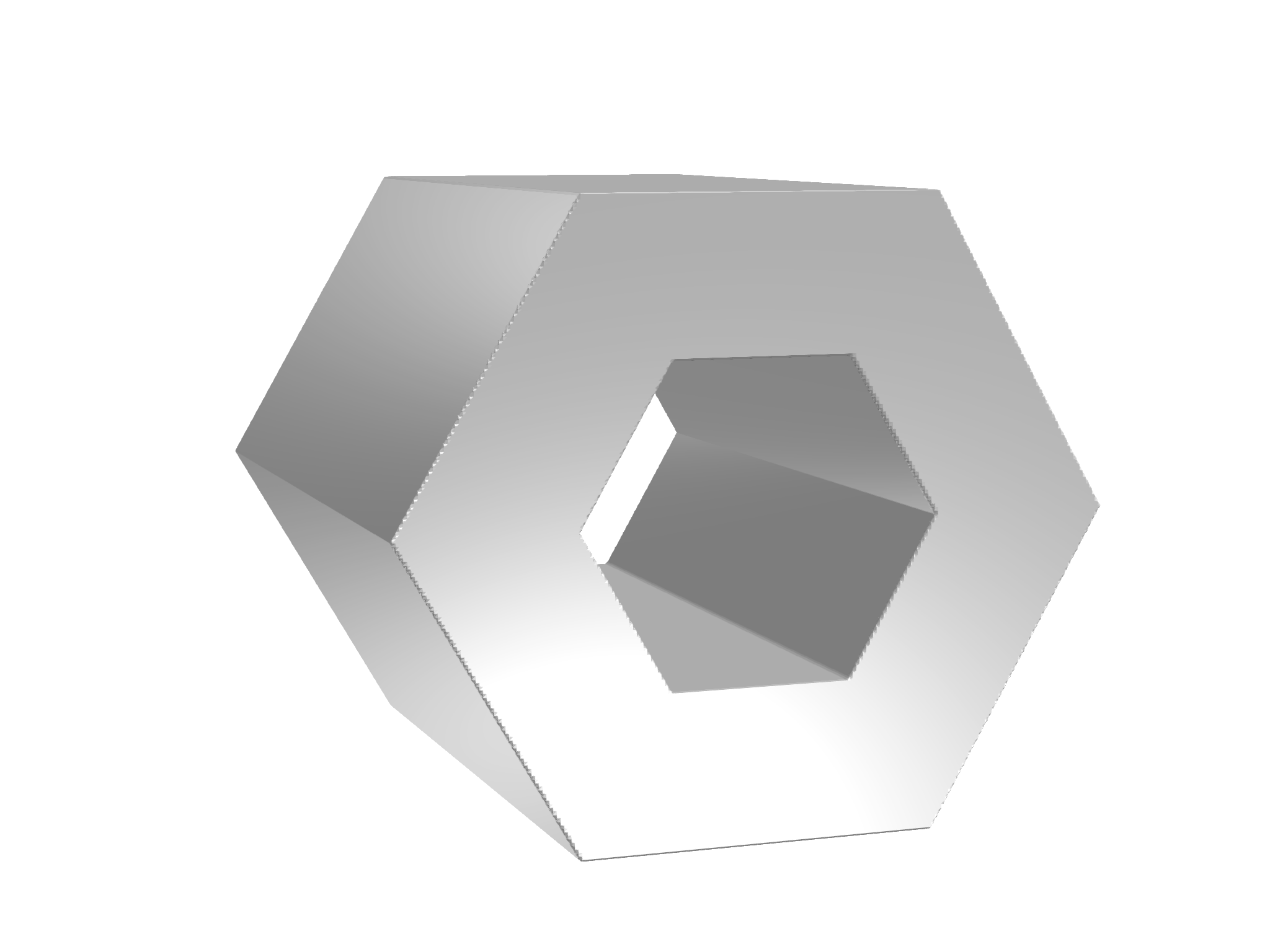
Figure 2. Torus $T_{r,R,h}$ for $n=3$ and $\tilde{\sigma}(p^{\prime})=|p^{\prime}|_{1}$ (left), and with hexagonal anisotropy (right).

We will use this set to construct a self-similar evolution

$$E_{t}:=\begin{cases}T_{r(t),R(t),h(t)},&0\leq t<t^{*},\\ \emptyset,&t\geq t^{*},\end{cases}$$

given appropriate functions $r(t)$, $R(t)$ and $h(t)$, where $t^{*}$ is the extinction time.

Let us first calculate the anisotropic curvature on the surface of $T_{r,R,h}$. We will split the surface $\Gamma=\partial T_{r,R,h}$ into (o) the outer surface $\Gamma_{\rm o}$ where $\tilde{\sigma}^{\circ}(x^{\prime})=R$, (i) the inner surface $\Gamma_{\rm i}$ where $\tilde{\sigma}^{\circ}(x^{\prime})=r$, and (s) the side facets $\Gamma_{\rm s}$ with $|x_{n}|=h$.

To compute the anisotropic curvature, we need to find a Cahn-Hoffman vector field $z:\Gamma\to{\mathbb{R}^{n}}$ on the surface such that $z(x)\in\partial\sigma(\nu(x))$ for $\mathcal{H}^{n-1}$-a.e. $x$ with minimal $\left\|\operatorname{div}_{\Gamma}z\right\|_{L^{2}(\Gamma)}$. It can be shown that $\operatorname{div}_{\Gamma}z$ minimizes the $L^{2}$ norm exactly when $\operatorname{div}_{\Gamma}z$ is constant on the flat parts of $\Gamma$, see [B10].

One such $z$ can be given explicitly as

(2.4) $$z(x)=\left(g(\tilde{\sigma}^{\circ}(x^{\prime}))x^{\prime},\frac{x_{n}}{h}\right),\qquad x=(x^{\prime},x_{n})\in\Gamma,$$

where

$$g(s):=as^{-n+1}+b,$$

with

$$a=-\frac{R^{n-2}r^{n-2}(R+r)}{R^{n-1}-r^{n-1}},\qquad b=\frac{R^{n-2}+r^{n-2}}{R^{n-1}-r^{n-1}}.$$

The constants $a$ and $b$ are chosen so that $g(r)r=-1$ and $g(R)R=1$. Since $r<R$ and $g(s)s$ is increasing in $s$ as $a<0$, we conclude that $-1<g(s)s<1$ for $r<s<R$. In particular,

(2.5) $$\tilde{\sigma}^{\circ}(g(\tilde{\sigma}^{\circ}(x^{\prime}))x^{\prime})\leq 1\Leftrightarrow g(\tilde{\sigma}^{\circ}(x^{\prime}))x^{\prime}\in\partial\tilde{\sigma}(0)\qquad\text{for all }x=(x^{\prime},x_{n})\in\Gamma.$$

Furthermore,

$$g^{\prime}(s)s+(n-1)g(s)=(n-1)b$$

and thus

(2.6) $$\begin{aligned} \operatorname{div}_{x^{\prime}}(g(\tilde{\sigma}^{\circ}(x^{\prime}))x^{\prime})&=g^{\prime}(\tilde{\sigma}^{\circ}(x^{\prime}))x^{\prime}\cdot\nabla\tilde{\sigma}^{\circ}(x^{\prime})+(n-1)g(\tilde{\sigma}^{\circ}(x^{\prime}))\\ &=g^{\prime}(\tilde{\sigma}^{\circ}(x^{\prime}))\tilde{\sigma}^{\circ}(x^{\prime})+(n-1)g(\tilde{\sigma}^{\circ}(x^{\prime}))=(n-1)b\end{aligned}$$

whenever $\nabla\tilde{\sigma}^{\circ}(x^{\prime})$ exists, where we used that $x^{\prime}\cdot\nabla\tilde{\sigma}^{\circ}(x^{\prime})=\tilde{\sigma}^{\circ}(x^{\prime})$, see [Rockafellar].

Let us check that $z$ is indeed a Cahn-Hoffman vector field on $\Gamma$. A convenient approach is to write $\Gamma$ as the level set of a Lipschitz continuous function. Consider

(2.7) $$\psi(x)=\max(r-\tilde{\sigma}^{\circ}(x^{\prime}),\tilde{\sigma}^{\circ}(x^{\prime})-R,|x_{n}|-h),\qquad x=(x^{\prime},x_{n})\in{\mathbb{R}^{n}}.$$

Clearly $\psi$ is Lipschitz, $\Gamma={\left\{x:\psi(x)=0\right\}}$ and $T_{r,R,h}={\left\{x:\psi(x)<0\right\}}$. $\nabla\psi$ is an outer normal vector of $\Gamma$ (with respect to $T_{r,R,h}$) and exists $\mathcal{H}^{n-1}$-a.e. on $\Gamma$. Since $\partial\sigma$ is positively zero-homogeneous, it is enough to show that $z(x)\in\partial\sigma(\nabla\psi(x))$ $\mathcal{H}^{n-1}$-a.e. $x\in\Gamma$.

Let $\operatorname{ri}\Gamma_{j}$ denote the relative interior of the surface $\Gamma_{j}$. Thus suppose that $x\in\Gamma$ such that $\nabla\psi(x)$ exists. We have three cases:

$x\in\operatorname{ri}\Gamma_{\rm o}$:

In a neighborhood of such a point, we see that $\psi(y)=\tilde{\sigma}(y^{\prime})-R$, and so in this case we have $\nabla\psi(x)=(\nabla\tilde{\sigma}^{\circ}(x^{\prime}),0)$, from which we deduce

$$z(x)=\left(\frac{x^{\prime}}{\tilde{\sigma}^{\circ}(x^{\prime})},\frac{x_{n}}{h}\right)\in\partial\tilde{\sigma}(\nabla\tilde{\sigma}^{\circ}(x^{\prime}))\times[-1,1]=\partial\sigma(\nabla\psi(x)).$$

$x\in\operatorname{ri}\Gamma_{\rm i}$:

This can be handled as the previous case, recalling that $\tilde{\sigma}$ is even and thus $-\frac{x^{\prime}}{\tilde{\sigma}^{\circ}(x^{\prime})}\in\partial\tilde{\sigma}(-\nabla\tilde{\sigma}^{\circ}(x^{\prime}))$.

$x\in\operatorname{ri}\Gamma_{\rm s}$:

Now we are on the top or the bottom flat facet, $\psi(y)=|y_{n}|-h$ in the neighborhood of this point, and so $\nabla\psi(x)=\left(0,\frac{x_{n}}{|x_{n}|}\right)$. Thus, recalling (2.5), we deduce

$$z(x)=\left(g(\tilde{\sigma}^{\circ}(x^{\prime}))x^{\prime},\frac{x_{n}}{|x_{n}|}\right)\in\partial\tilde{\sigma}(0)\times{\left\{\frac{x_{n}}{|x_{n}|}\right\}}=\partial\sigma(\nabla\psi(x)).$$

We have proved that $z$ defined in (2.4) is a Cahn-Hoffman field on $\Gamma$.

Now we show that $\operatorname{div}_{\Gamma}z$ is constant on the flat parts of $\Gamma$, and hence it minimizes $\left\|\operatorname{div}_{\Gamma}z\right\|_{L^{2}(\Gamma)}$. The surface (tangential) divergence $\operatorname{div}_{\Gamma}z(x)$ for $x\in\Gamma$ can be computed easily using the level set method by constructing an extension $\bar{z}$ of $z$ away from the facet such that $\bar{z}\in\partial\sigma(\nabla\psi)$ a.e. in a neighborhood of $x\in\Gamma$ so that $\operatorname{div}\bar{z}(x)$ exists. Then we have $\operatorname{div}_{\Gamma}z(x)=\operatorname{div}\bar{z}(x)$, see [G06].

Following the above verification that $z$ is a Cahn-Hoffman vector field, we can construct the extension $\bar{z}$ in a neighborhood of $x\in\Gamma$ in the following three cases in the following way:

$x\in\operatorname{ri}\Gamma_{\rm o}$:

Here we can simply take $\bar{z}(y)=\left(\frac{y^{\prime}}{\tilde{\sigma}^{\circ}(y^{\prime})},\frac{y_{n}}{h}\right)$ which yields

$$\operatorname{div}_{\Gamma}z(x)=\operatorname{div}\bar{z}(x)=\frac{n-2}{R}+\frac{1}{h},$$

if the divergence exists, where we followed the computation in (2.6) with $g(s)=\frac{1}{s}$.

$x\in\operatorname{ri}\Gamma_{\rm i}$:

Similarly to the previous situation, we may take

$$\bar{z}(y)=\left(-\frac{y^{\prime}}{\tilde{\sigma}^{\circ}(y^{\prime})},\frac{y_{n}}{h}\right),$$

which yields

$$\operatorname{div}_{\Gamma}z(x)=\operatorname{div}\bar{z}(x)=-\frac{n-2}{r}+\frac{1}{h}$$

if the divergence exists.

$x\in\operatorname{ri}\Gamma_{\rm s}$:

Here we may take $\bar{z}(y)=\left(g(\tilde{\sigma}^{\circ}(y^{\prime}))y^{\prime},\frac{y_{n}}{|y_{n}|}\right)$, yielding

$$\operatorname{div}_{\Gamma}z(x)=\operatorname{div}\bar{z}(x)=(n-1)b$$

using (2.6).

Since $\operatorname{div}_{\Gamma}z$ is constant on the flat parts of the surface, we deduce that it minimizes the $L^{2}$ norm among all Cahn-Hoffman vector fields and therefore we can define $\kappa_{\sigma}=-\operatorname{div}_{\Gamma}z$.

Let us now find the normal velocity $V$ of the surface $\Gamma_{t}=\partial T_{r(t),R(t),h(t)}$ where $r(t)$, $R(t)$ and $h(t)$ are some $C^{1}$ functions satisfying $0<r(t)<R(t)$, $0<h(t)$. It is straightforward to use the level set method. Let $\psi(x,t)$ be the function defined in (2.7) with the time dependent parameters $r(t)$, $R(t)$, $h(t)$ above. Let us fix $t$ and $x\in\Gamma_{t}$ so that $\psi_{t}(x,t)$ and $\nabla\psi(x,t)$ are defined. We can again consider three cases and use the formula $V(x,t)=-\frac{\psi_{t}}{|\nabla\psi|}(x,t)$ [G06]:

(2.8) $$V(x,t)=\begin{cases}\frac{R^{\prime}(t)}{|\nabla\tilde{\sigma}^{\circ}(x^{\prime})|},&x\in\operatorname{ri}\Gamma_{\rm o},\\ -\frac{r^{\prime}(t)}{|\nabla\tilde{\sigma}^{\circ}(x^{\prime})|},&x\in\operatorname{ri}\Gamma_{\rm i},\\ h^{\prime}(t),&x\in\operatorname{ri}\Gamma_{\rm s}.\end{cases}$$

To relate $V$ to $\kappa_{\sigma}$ using the law (2.3), it is left to compute $\beta(\nu)$ on $\Gamma$. Using the level set method again, $\nu=\frac{\nabla\psi}{|\nabla\psi|}$ whenever $\nabla\psi$ exists and is nonzero [G06], and therefore

(2.9) $$\nu(x)=\begin{cases}\frac{(\nabla\tilde{\sigma}^{\circ}(x^{\prime}),0)}{|\nabla\tilde{\sigma}^{\circ}(x^{\prime})|},&x\in\operatorname{ri}\Gamma_{\rm o},\\ -\frac{(\nabla\tilde{\sigma}^{\circ}(x^{\prime}),0)}{|\nabla\tilde{\sigma}^{\circ}(x^{\prime})|},&x\in\operatorname{ri}\Gamma_{\rm i},\\ (0,\frac{x_{n}}{|x_{n}|}),&x\in\operatorname{ri}\Gamma_{\rm s}.\end{cases}$$

Recalling $\beta$ given in (2.2) and that $\tilde{\sigma}(\pm\nabla\tilde{\sigma}^{\circ}(x^{\prime}))=1$ whenever $\nabla\tilde{\sigma}^{\circ}(x^{\prime})$ exists [Rockafellar], we deduce

(2.10) $$\beta(\nu(x))=\begin{cases}\frac{1}{|\nabla\tilde{\sigma}^{\circ}(x^{\prime})|},&x\in\operatorname{ri}\Gamma_{\rm o}\cup\operatorname{ri}\Gamma_{\rm i},\\ \mu,&x\in\operatorname{ri}\Gamma_{\rm s}.\end{cases}$$

Relating the anisotropic curvature $\kappa_{\sigma}=-\operatorname{div}_{\Gamma}z$ with (2.8), (2.9) and (2.10) via (2.3), we must have

(2.11) $$\begin{aligned} R^{\prime}&=-\frac{n-2}{R}-\frac{1}{h},\\ r^{\prime}&=-\frac{n-2}{r}+\frac{1}{h},\\ h^{\prime}&=-(n-1)\mu\frac{R^{n-2}+r^{n-2}}{R^{n-1}-r^{n-1}}.\end{aligned}$$

For the evolution to be self-similar, we therefore need

$$\left(\frac{r}{R}\right)^{\prime}=0=\left(\frac{h}{R}\right)^{\prime}.$$

Thus there are constants $\gamma\in(0,1)$ and $\lambda>0$ such that

$$r=\gamma R,\qquad h=\lambda R.$$

Plugging this into (2.11) and multiplying each equation by $R$, we get

(2.12a) $$RR^{\prime} =-(n-2)-\frac{1}{\lambda}$$

(2.12b) $$=-\frac{n-2}{\gamma^{2}}+\frac{1}{\lambda\gamma}$$

(2.12c) $$=-\frac{(n-1)\mu}{\lambda}\cdot\frac{1+\gamma^{n-2}}{1-\gamma^{n-1}}.$$

From (2.12a) and (2.12b), we obtain

(2.13) $$\lambda=\frac{\gamma}{(n-2)(1-\gamma)}.$$

On the other hand, (2.12a) and (2.12c) yield

(2.14) $$\lambda=\frac{1}{n-2}\left((n-1)\mu\frac{1+\gamma^{n-2}}{1-\gamma^{n-1}}-1\right).$$

Hence combining (2.13) and (2.14) and multiplying both sides by $(n-2)(1-\gamma^{n-1})$, we have

$$1+\gamma+\cdots+\gamma^{n-2}=(n-1)\mu(1+\gamma^{n-2}).$$

This equation has a solution $\gamma\in(0,1)$ only for certain $\mu$. Let us only consider $n=3$. Then we have

$$0=(2\mu-1)(1+\gamma),$$

which has a solution $\gamma\in(0,1)$ only if $\mu=\frac{1}{2}$. In this case there are infinitely many solutions, for instance,

$$\gamma=\tfrac{1}{2},\quad\lambda=1.$$

Then the solution of (2.3) with initial data $E_{0}=T_{\frac{1}{2},1,1}$ is the self-similar evolution

$$E_{t}=\begin{cases}\sqrt{1-4t}E_{0},&0\leq t<t^{*}=\frac{1}{4},\\ \emptyset,&t^{*}\leq t.\end{cases}$$

It is possible to show that this is the unique (open) evolution given by the viscosity solution of (2.3) in the sense of [GP_CPAM], but this is beyond the scope of this note. For more details, see [GGGakuto].

2.3. The sponge

In this section we construct a shrinking “sponge” in dimension $n=3$. It is a self similar solution of the crystalline mean curvature flow with cubic anisotropy $\sigma(p)=|p|_{1}$ with genus $5$ and resembles the level $1$ Menger sponge. Its shape is given by a cube centered at the origin from which the neighborhood (in the maximum ($\ell^{\infty}$) norm) of all three axes has been removed, see Figure 3. It is an analogue of the solution that was discovered numerically by D. L. Chopp [Chopp] for the standard isotropic mean curvature flow.

Let us thus consider the crystalline mean curvature flow

(2.15) $$V=\sigma(\nu)\kappa_{\sigma}$$

where $\sigma(p)=|p|_{1}$ is the cubic ($\ell^{1}$) anisotropy, with initial data

(2.16) $$E_{0}:=S_{r_{0},R_{0}}$$

for some constants $0<r_{0}<R_{0}$, where

$$S_{r,R} :={\left\{x\in\mathbb{R}^{3}:|x|_{\infty}<R,\ |x_{i}|>r\text{ for at least two of $i=1,2,3$}\right\}}$$

for $0<r<R$, see Figure 3.

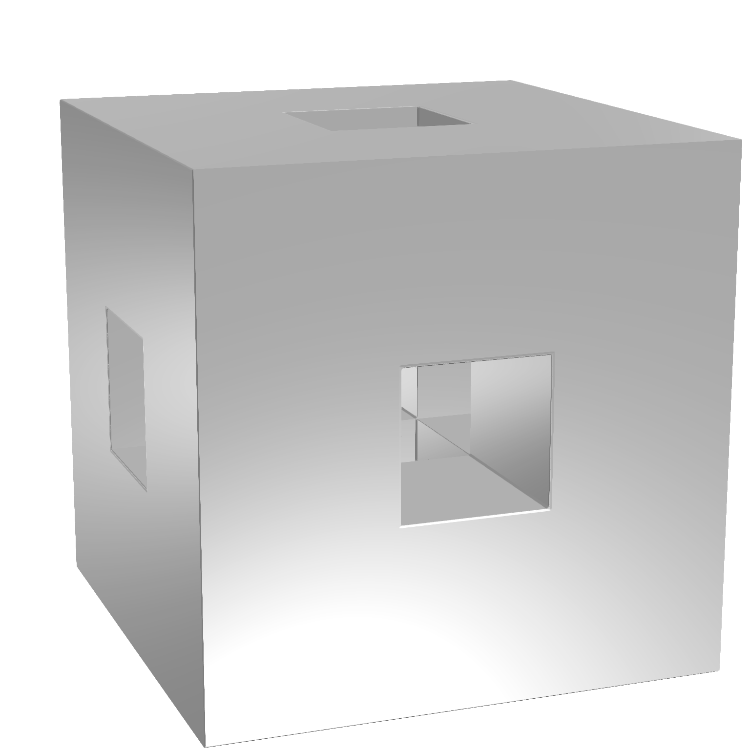
(a)

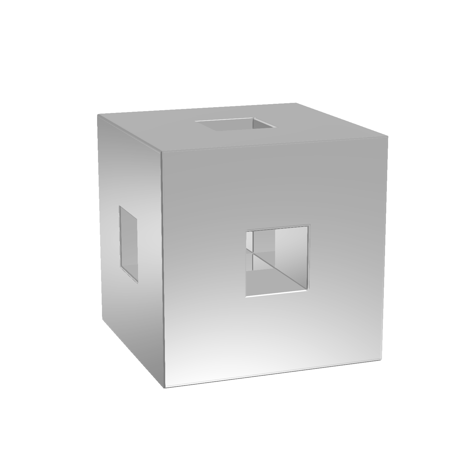
(b)

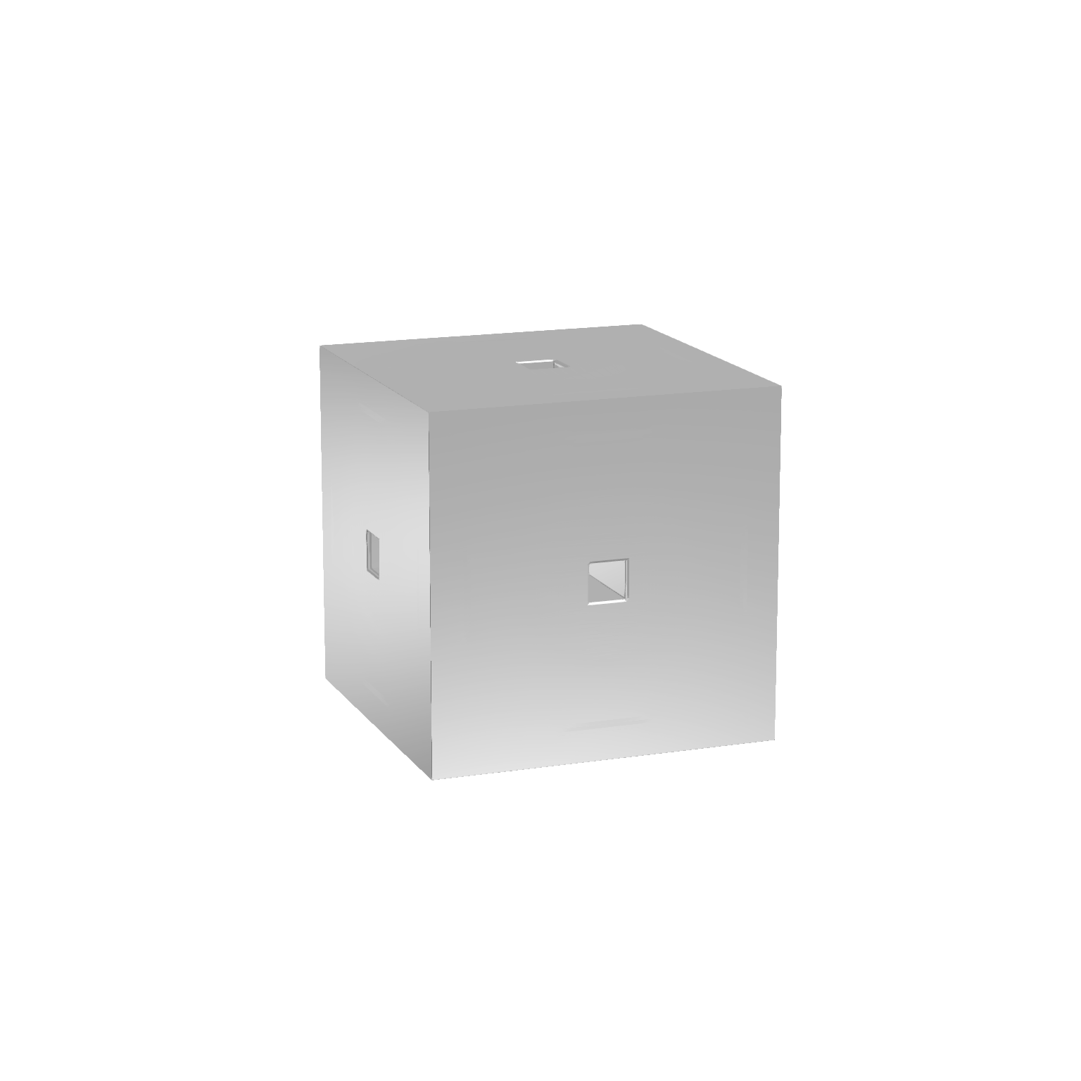
(c)

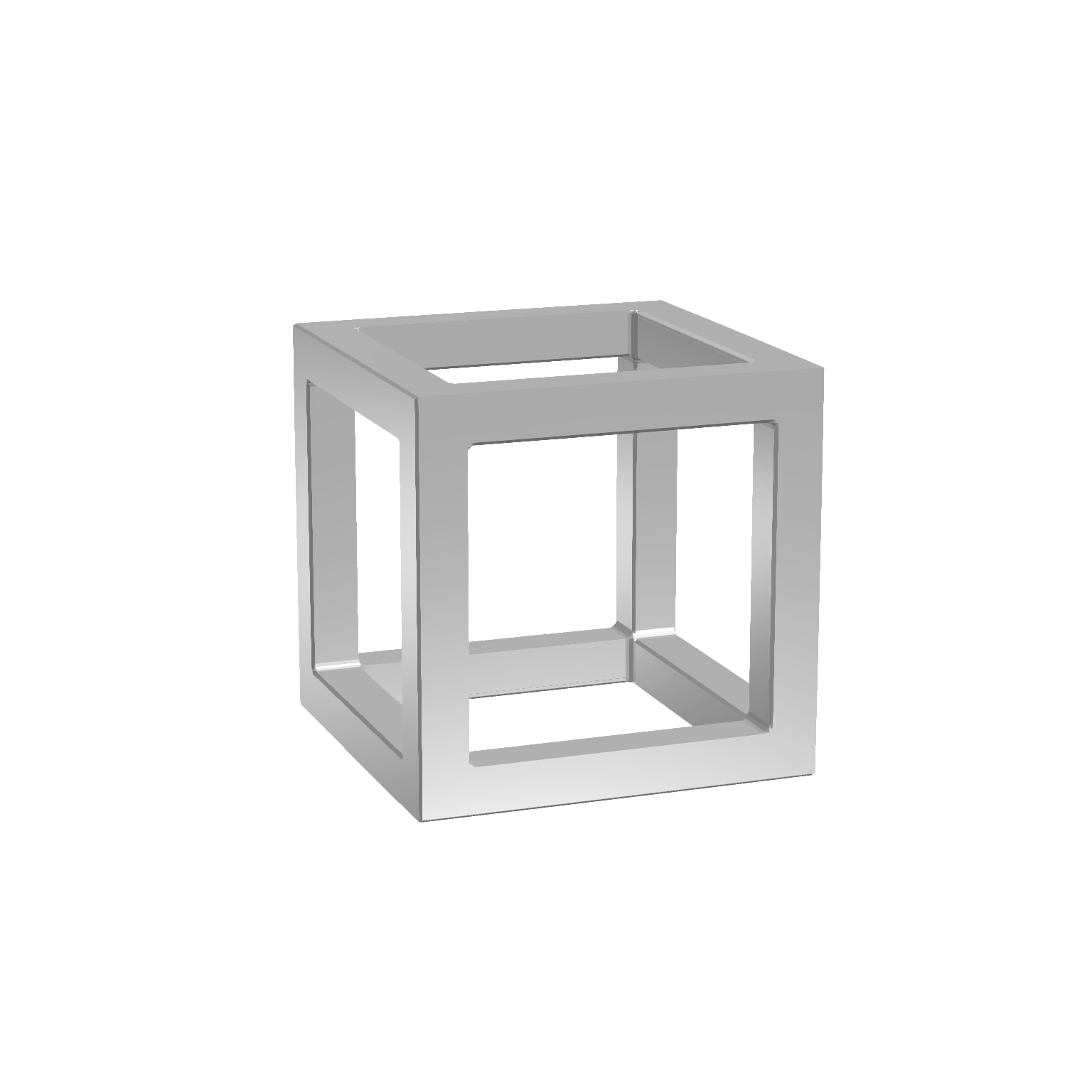
(d)

Figure 3. The shrinking sponge. (A) The initial set $E_{0}$. The outer edge has length $2R_{0}$ while the inner edge has length $2r_{0}$. (B) Self-similar sponge solution with initial size $0.8$ at time $t=0.015$ computed with domain resolution $M=256$. A numerical solution uses Chambolle’s algorithm; since the solution is unstable, the accumulated numerical errors will cause it to eventually diverge from the self-similar solution. (C) Evolution for $\frac{R_{0}}{r_{0}}>\xi^{*}$. (D) Evolution for $\frac{R_{0}}{r_{0}}<\xi^{*}$.

We claim that the open evolution ${\left\{E_{t}\right\}}_{t\geq 0}$ solving (2.15) is of the form

$$E_{t}:=S_{r(t),R(t)},$$

where $r(t)$, $R(t)$ are solutions of a certain ODE system. Our goal is to find $0<r_{0}<R_{0}$ so that the evolution ${\left\{E_{t}\right\}}_{t\geq 0}$ is self-similar.

For $0<r<R$, due to the symmetries, $S_{r,R}$ has only exactly two types of facets: (o) the outer facet given by a square of side $2R$ with square of side $2r$ with the same center removed, and (i) the inner facet given by a rectangle with sides of lengths $2r$ and $R-r$. The crystalline curvature on each of these facets can be expressed as the ratio of their signed perimeter and their area, that is,

$$\kappa_{\textrm{o}} =-\frac{8(R+r)}{4R^{2}-4r^{2}}=-\frac{2}{R-r}, \kappa_{\textrm{i}} =\frac{1}{r}-\frac{2}{R-r}=\frac{R-3r}{r(R-r)}.$$

For a detailed explanation of why these are indeed the curvatures, see Section 2.2 for an explicit Cahn-Hoffman field construction, or [LMM].

Following the reasoning in Section 2.2, the normal velocity of the outer facet of ${\left\{E_{t}\right\}}$ is $V=R^{\prime}(t)$ and the inner facet is $V=-r^{\prime}(t)$. Note also that since the facets of $S_{r,R}$ are axes-aligned, we have $\sigma(\nu)=|\nu|_{1}=1$ a.e. on $\partial S_{r,R}$. Therefore (2.15) simplifies for ${\left\{E_{t}\right\}}$ into the system of ODEs

(2.17) $$\left\{\begin{aligned} R^{\prime}&=\kappa_{\textrm{o}}=-\frac{2}{R-r},\\ r^{\prime}&=-\kappa_{\textrm{i}}=-\frac{R-3r}{r(R-r)},\end{aligned}\right.\qquad t>0,$$

with initial data $r(0)=r_{0}$, $R(0)=R_{0}$.

Let us perform a more detailed analysis of the behavior of the system (2.17). The evolution will be self-similar if

$$\xi(t):=\frac{R(t)}{r(t)}\equiv const.$$

Rewriting the system (2.17) for $\xi$ and $r$, we have

(2.18) $$\left\{\begin{aligned} \xi^{\prime}&=\frac{\xi^{2}-3\xi-2}{r^{2}(\xi-1)},\\ r^{\prime}&=-\frac{\xi-3}{r(\xi-1)},\end{aligned}\right.\qquad t>0,$$

with initial data $\xi_{0}=\frac{R_{0}}{r_{0}}>1$, $r(0)=r_{0}>0$.

We set

$$g(\xi):=\xi^{2}-3\xi-2.$$

The constant $\xi^{*}:=\frac{3+\sqrt{17}}{2}$ is the unique value $>1$ such that $g(\xi^{*})=0$. Let us also introduce $Q_{R}:={\left\{x\in\mathbb{R}^{3}:|x|_{\infty}<R\right\}}$

We can classify the behavior of the solution of (2.18) according to the initial ratio $\xi_{0}=\frac{R_{0}}{r_{0}}$ as follows:

1. $1<\xi_{0}<\xi^{*}$: Since $\xi^{\prime}<0$ and $r(t)\leq R_{0}$, there exists a time $t^{*}>0$ such that $\lim_{t\to t^{*}-}\xi(t)=1$, that is, $\lim_{t\to t^{*}-}R(t)-r(t)=0$. The sponge gets thinner with time and converges to the edges of the cube $Q_{R(t^{*})}$, and vanishes at $t^{*}$; Figure 3(D).

2. $\xi_{0}=\xi^{*}$: The solution is $\xi(t)=\xi_{0}=\xi^{*}$, $r(t)=\sqrt{r_{0}^{2}-2ct}$ for $0<t<t^{*}$, where $c=\frac{\xi^{*}-3}{\xi^{*}-1}>0$ and $t^{*}=\frac{r_{0}^{2}}{2c}>0$. At $t=t^{*}$ the sponge vanishes. The evolution is self-similar.

3. $\xi_{0}>\xi^{*}$: There is time $t^{\Box}>0$ such that $\lim_{t\to t^{\Box}-}(\xi(t),r(t),R(t))=(+\infty,0,R(t^{\Box}))$. In this case, the holes close up and the sponge becomes a cube at time $t^{\Box}$; Figure 3(D). After $t=t^{\Box}$, $R$ evolves with $R^{\prime}=-\frac{2}{R}$. The cube vanishes at a later time $t^{*}>t^{\Box}$.

See Figure 3 for a numerical solution using Chambolle’s algorithm discussed in Section 3. Note that (b) is unstable since $g^{\prime}(\xi^{*})>0$, and therefore numerically we will observe either (a) or (c).

Let us summarize the solution of (2.15) in terms of the values $0<r_{0}<R_{0}$:

$1<\frac{R_{0}}{r_{0}}\leq\xi^{*}$:

$$E_{t}:=\begin{cases}S_{r(t),R(t)},&0\leq t<t^{*},\\ \emptyset,&t\geq t^{*}.\end{cases}$$

$\frac{R_{0}}{r_{0}}>\xi^{*}$:

$$E_{t}:=\begin{cases}S_{r(t),R(t)},&0\leq t<t^{\Box},\\ Q_{R(t)},&t^{\Box}\leq t<t^{*},\\ \emptyset,&t\geq t^{*}.\end{cases}$$

As in the shrinking doughnut case by following [GGGakuto], one can show that this is the unique (open) evolution given by the viscosity solution of (2.15) in the sense of [GP_CPAM].

3. The numerical algorithm

An efficient method for the mean curvature flow (1.2) is based on a minimizing movement formulation due to A. Chambolle [Chambolle], which can be efficiently solved by a split Bregman iteration proposed by [GO, OOTT]. Suppose that $\Omega\subset{\mathbb{R}^{n}}$ is a bounded convex domain and that the evolving set is contained in $\Omega$. Furthermore, we need to assume that the one-homogeneous extension of $\beta$ as in (1.1) is convex.

The insight of Chambolle is to formulate the minimizing scheme of F. Almgren, J. E. Taylor and L. Wang [ATW] in terms of the signed distance function, so that the evolving set is its level set. In [Chambolle], he proposed the time discretization by the minimization problem ($f\equiv 0$ in [Chambolle])

(3.1) $$v_{m+1}\leftarrow\operatorname*{arg\,min}_{v\in L^{2}(\Omega)}\left(\frac{1}{2h}\left\|v-w_{m}\right\|^{2}+\int_{\Omega}\sigma(Dv)\;dx-{\left\langle f_{m},v\right\rangle}\right),$$

where $h>0$ is a chosen time step, $w_{m}$ is the signed distance function of the level set ${\left\{v_{m}<0\right\}}$ at the previous time step $m$, induced by the metric given by the mobility $\beta$ and $f_{m}=f(\cdot,mh)$. The minimization is performed over all $v\in L^{2}(\Omega)$, and $\left\|\cdot\right\|$ and ${\left\langle\cdot,\cdot\right\rangle}$ are the $L^{2}(\Omega)$-norm and inner product, respectively. The total variation energy $\int_{\Omega}\sigma(Dv)\;dx$ is defined as the $L^{2}$ lower semicontinuous envelope of the functional $v\mapsto\int_{\Omega}\sigma(\nabla v)\;dx$ defined for $v$ in the Sobolev space $W^{1,1}(\Omega)$. Note that the functional in (3.1) is the Moreau-Yosida regularization of the total variation energy with parameter $h$, and the minimization problem (3.1) is equivalent to the resolvent problem for the total variation energy. In other words, it is the implicit Euler discretization of the total variation flow [ACM]. Since $\left|\nabla v_{m+1}\right|\approx\left|\nabla w_{m}\right|=1$ when $h$ is small, we can deduce that $\frac{v_{m+1}-w_{m}}{h}\approx V$ using (2.1).

The full minimizing movements algorithm to find a discrete sequence of approximations $E_{m}$, $m=0,1,2,\ldots$ of the evolving set ${\left\{E_{t}\right\}}_{t\geq 0}$ at time steps $t_{m}=mh$ reads: Set $E_{0}$ as the initial data and then iteratively for $m=0,\ldots$ do

(3.2) $$\begin{aligned} w_{m}&\leftarrow\operatorname{signdist}_{\beta}E_{m}\\ v_{m+1}&\leftarrow\operatorname*{arg\,min}_{v\in L^{2}(\Omega)}\left(\frac{\mu}{2}\left\|v-w_{m}\right\|^{2}+\left\|\sigma(\nabla v)\right\|_{1}-{\left\langle f_{m},v\right\rangle}\right),\\ E_{m+1}&\leftarrow{\left\{v_{m+1}<0\right\}},\end{aligned}$$

where $\mu=\frac{1}{h}$, and $f$ is a given source, and we write $\left\|\sigma(\nabla v)\right\|_{1}=\int_{\Omega}\sigma(Dv)\;dx$. Note that the minimization is equivalent to the minimization of

$$\frac{\mu}{2}\left\|v-(w_{m}+\mu^{-1}f_{m})\right\|^{2}+\left\|\sigma(\nabla v)\right\|_{1}.$$

The signed distance function must correspond to the anisotropy $\beta$. Recall that we assume that $\beta$ is one-homogeneously extended to ${\mathbb{R}^{n}}$ as in (1.1), and such a extension is an anisotropy. In particular, $\beta$ is assumed to be convex (but it needs not to be symmetric with respect to the origin). We define the signed distance as

$$\operatorname{signdist}_{\beta}E_{m}(x) :=\inf_{y\in E_{m}}\beta^{\circ}(x-y)-\inf_{y\in E_{m}^{\textsf{c}}}\beta^{\circ}(y-x)$$

$$\ =\begin{cases}\inf_{y\in E_{m}}\beta^{\circ}(x-y),&x\notin E_{m},\\ -\inf_{y\in E_{m}^{\textsf{c}}}\beta^{\circ}(y-x),&x\in E_{m},\end{cases}$$

where $\beta^{\circ}(x):=\sup{\left\{x\cdot p:\beta(p)\leq 1\right\}}$ is the convex polar of $\beta$. If $\beta(p)=|p|$, $\operatorname{signdist}_{\beta}$ is just the standard signed distance function induced by the Euclidean metric.

Let us motivate the above choice of $w_{m}$. If we set $w_{m}$ to be the signed distance above, we have $\beta(\nabla w_{m})=1$ a.e., see [Rockafellar]. Then performing (3.2), $v_{m+1}-w_{m}$ is approximately $(\kappa-f_{m})h$ and the free boundary advances in the normal direction by

$$-\frac{(\kappa-f_{m})h}{|\nabla w_{m}|}=-\beta\left(\frac{\nabla w_{m}}{|\nabla w_{m}|}\right)(\kappa-f_{m})h=\beta(\nu)(-\kappa+f_{m})h$$

yielding the correct free boundary velocity.

As $h\to 0$, the evolution will converge to a continuous evolution ${\left\{E_{t}\right\}}_{t\geq 0}$, see [Chambolle]. Provided that there is no fattening, this evolution will be the unique solution of the anisotropic mean curvature flow [CMP, CMNP, Ishii14] and, in the crystalline case in particular, the unique viscosity solution solution of the crystalline mean curvature flow [GP16, GP_CPAM].

It might seem that the minimization problem in (3.2) is rather difficult for numerical computation, mainly due to the non-differentiable second term. In particular, the standard minimization methods like conjugate gradients or Newton iteration are poorly suited. For this reason, Chambolle proposed an iterative algorithm in [Chambolle]. More recently, it was recognized in [OOTT] that the minimization problem can be addressed by the so-called proximal algorithms [ParikhBoyd], the alternative direction method of multipliers (ADMM) or the split Bregman method [GO]. To find the minimizer $v$ of $\frac{\mu}{2}\left\|v-u\right\|^{2}+\left\|\sigma(\nabla v)\right\|_{1}$, we choose $\lambda>0$, set $b_{0}=d_{0}=0$ and then iterate for $k=0,1,\ldots$

(3.3a) $$v_{k+1} \leftarrow\operatorname*{arg\,min}_{v}\frac{\mu}{2}\left\|v-u\right\|^{2}+\frac{\lambda}{2}\left\|d_{k}-\nabla v-b_{k}\right\|^{2},$$

(3.3b) $$d_{k+1} \leftarrow\operatorname*{arg\,min}_{d}\left\|\sigma(d)\right\|_{1}+\frac{\lambda}{2}\left\|d-\nabla v_{k+1}-b_{k}\right\|^{2},$$

(3.3c) $$b_{k+1} \leftarrow b_{k}+\nabla v_{k+1}-d_{k+1},$$

until some stopping condition is reached, typically when $\left\|v_{k+1}-v_{k}\right\|_{2}$ is sufficiently small. Heuristically, this scheme introduces a new gradient variable $d$, and then enforces the constraint $d=\nabla v$ by a quadratic penalty. Since we are minimizing a sum of convex terms over two variables, the problems can be decoupled into iterating (3.3a) and (3.3b). (3.3c) is called a Bregman iteration, and it helps to enforce the constraint exactly. Note that when convergence is achieved, (3.3c) implies $d=\nabla v$. For a detailed discussion of the motivation, convergence and other properties, see [GO].

The advantage of this iteration process is the simplicity of the subproblems. The first minimization problem (3.3a) is equivalent to finding the solution $v$ of

(3.4) $$(\mu-\lambda\Delta)v=\mu u+\lambda\operatorname{div}(b_{k}-d_{k})\qquad\text{in $\Omega$},$$

with an appropriate boundary condition, for instance Neumann. It is not necessary to solve it accurately, so one or two Gauss-Seidel iterations are sufficient [GO].

To find a numerical solution, we use the finite difference method (FDM) or the finite element method (FEM) to discretize (3.2), see Section 3.1. In both cases, we represent $d,b$ by discrete values on the lattice (FDM) or on the elements (FEM). This has the important consequence that the minimization problem (3.3b) for $d$ in the discrete case completely decouples. Then, for each node or element $i$ the $i$th component of the minimizer $d_{k+1,i}$ is given by the so-called shrink operator [GO]

(3.5) $$d_{k+1,i}=\operatorname{shrink}_{\sigma}((\nabla v_{k+1}+b_{k})_{i},1/\lambda).$$

Note that the shrink operator can be expressed using the orthogonal projection on the Wulff shape $\mathcal{W}$ of $\sigma$ [OOTT],

$$\operatorname{shrink}_{\sigma}(\xi,1/\lambda):=(I-P_{\mathcal{W}/\lambda})(\xi).$$

In typical cases of isotropic, cubic and hexagonal anisotropies, that is, when the Wulff shape $\mathcal{W}$ is a sphere, a cube or a hexagonal prism, respectively, the orthogonal projection is very simple. More general Wulff shapes can be handled by the method proposed in [OOTT].

It is interesting to relate the Bregman iterate $b$ to the Cahn-Hoffman vector field in the definition of the anisotropic (crystalline) mean curvature. In particular, for a node or an element $i$, if convergence is achieved, (3.5) yields $d_{i}=\operatorname{shrink}_{\sigma}(d_{i}+b_{i},1/\lambda)$ and we have $b_{i}=P_{\mathcal{W}/\lambda}(d_{i}+b_{i})$. From the last equality, we see that either $d_{i}=0$, but then $\lambda b_{i}\in\mathcal{W}$, or $d_{i}\neq 0$, but then $\lambda b_{i}\in\partial\mathcal{W}$ and $d_{i}$ is a normal of $\partial\mathcal{W}$ at $\lambda b_{i}$. In other words, $\lambda b_{i}\in\partial\sigma(d_{i})$. From (3.4) we deduce that $\frac{v-u}{h}=\lambda\operatorname{div}b$. Hence $\lambda b$ is a discrete Cahn-Hoffman vector field for the resolvent problem (3.1).

3.1. Discretization: FDM vs FEM

The standard way [GO, OOTT] to discretize (3.3) is to use the finite difference method (FDM). This is quite straightforward, see also [Chambolle], and seems sufficient in two dimensions and for applications in image processing. For instance, (3.4) is discretized using the standard central difference scheme on a $2n+1$ point stencil. However, in three dimensions this approach introduces unwanted artifacts, for instance rounding of edges in certain directions, see Figure 4.

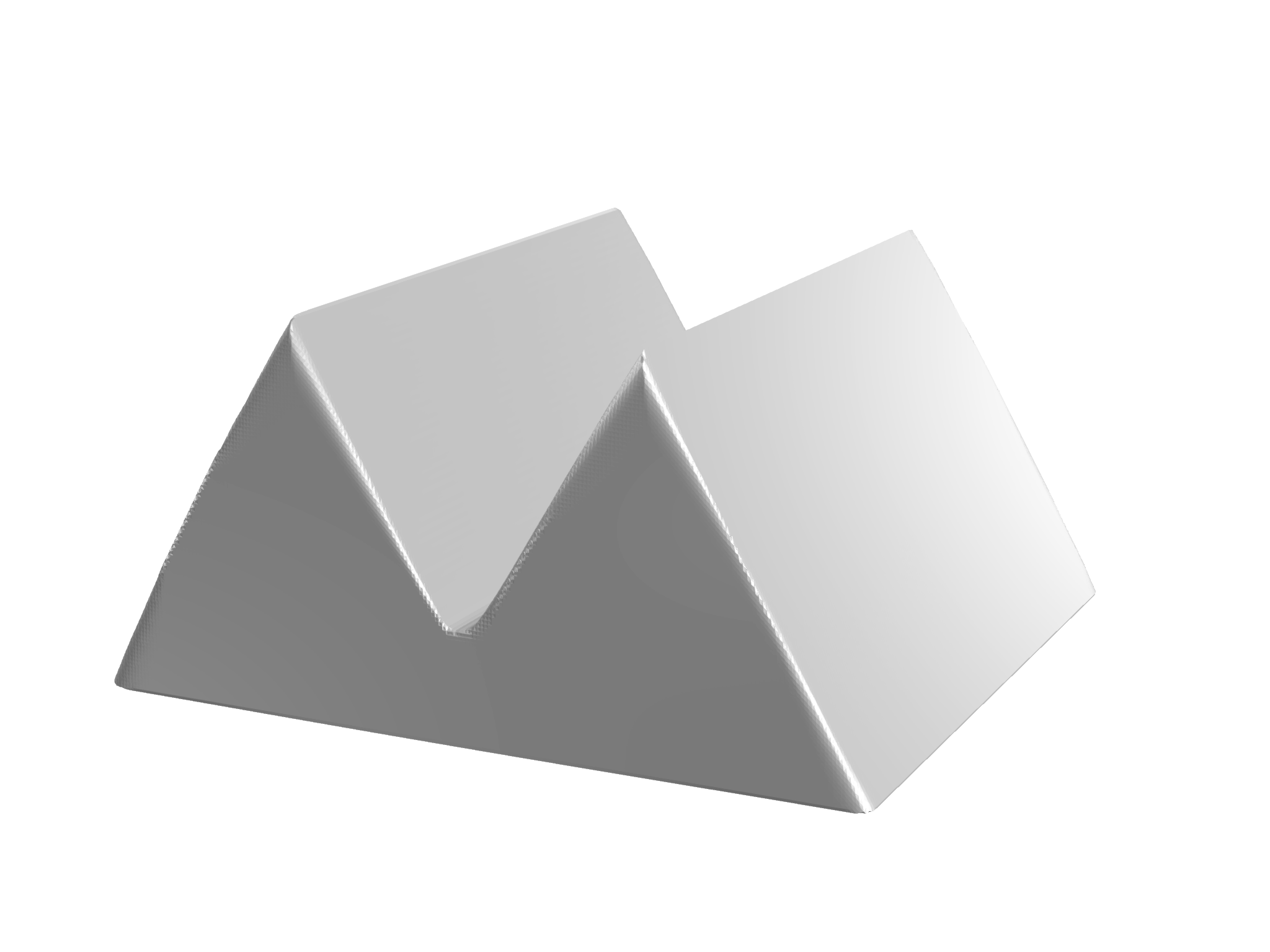
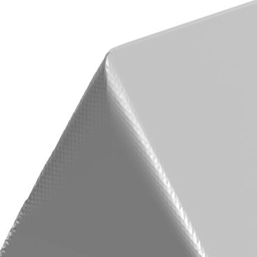
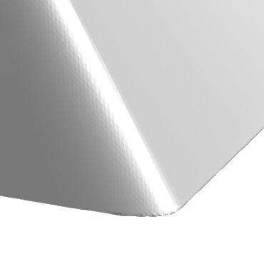
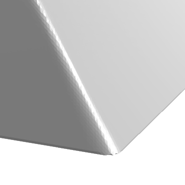
Figure 4. Rounding of edges in the computation in Figure 18; neighborhood of the top left vertex (top row) and bottom right vertex (bottom row) are magnified: FDM (left column) vs. FEM (right column).

This is most likely caused by the fact that the gradient $d$ and the Cahn-Hoffman vector field $b$ on a given cubic cell are given only by four out of the eight nodes. This restriction of the number of degrees of freedom for the gradient limits the ability of the discretization to account for a rapidly changing vector field near an edge.

We propose a finite element method (FEM) discretization. We minimize the functional in (3.3a) on the space of piece-wise linear functions ($P^{1}$ elements) on a tetrahedral mesh. The vector fields $\nabla v$, $d$ and $b$ are then approximated by piece-wise constant vector fields ($P^{0}$ elements) on this mesh. The minimization problem (3.3b) on the space of piece-wise constant ($P^{0}$ elements) completely decouples on each element and the minimizer is given by (3.5).

The merit of this approach is the six-fold increase of the number of degrees of freedom of $d$ and $b$ (for the cost of also increasing the memory and computational time requirements), which allows for a better resolution of edges, see Figure 4. Additionally, it is consistent with our redistance approach in Section 3.2. However, at some extreme cases in two dimensions the FEM performs worse than FDM, see Figure 5 for an example.

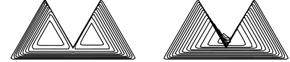
Figure 5. A triangular anisotropy demonstrates a topological change in 2D for non-even anisotropies. Left: FDM Right: FEM. Parameters $h=10^{-4}$, $M=64$, and plot step $0.005=50h$.

Let us present the mesh construction in an arbitrary dimension to fix the idea. We assume that the computational domain is a cube $\Omega$ is subdivided into $M^{n}$ smaller cubes of equal size, $M\in\mathbb{N}$ is the resolution. We split each of the smaller cubes into $n!$ simplices in the following way. By translation and scaling, we may assume that the small cube is $Q=[0,1]^{n}$. Let ${\left\{p_{m}\right\}}_{m=1}^{n!}$ be the $n!$ permutations of $(1,\ldots,n)$. For each $m=1,\ldots,n!$, we define the sequence of $n+1$ vertices $\xi_{m,1},\ldots,\xi_{m,n+1}$ of $Q$ using

$$\xi_{m,1} =(0,\ldots,0),$$

$$(\xi_{m,j+1})_{i} =\begin{cases}(\xi_{m,j})_{i}+1&\text{if $i=(p_{m})_{j}$,}\\ (\xi_{m,j})_{i}&\text{otherwise},\end{cases}\qquad i=1,\ldots,n.$$

Then their convex hulls,

$$\operatorname{conv}(\xi_{m,1},\ldots,\xi_{m,n+1}),\qquad 1\leq m\leq n!,$$

are simplices that form a tessellation of $Q$, see Figure 6.

Figure 6. Tessellation of the unit cube in $n=2$.

We use the mesh that is given by the above tessellation of each of the $M^{n}$ cubes in $\Omega$. The total number of elements is $n!M^{n}$.

3.2. Redistance

At each time step of the algorithm (3.2), the signed distance function $\operatorname{signdist}_{\beta}{\left\{v_{m}<0\right\}}$ to the $0$-level set of the solution of the minimization problem has to be recomputed. (This is not strictly true, see the discussion in Section 3.3.) It is sometimes referred to as redistance. The problem amounts to solving the (anisotropic) eikonal equation $|\nabla w|_{\beta}:=\beta^{\circ}(\nabla w)=1$ with boundary data $w=0$ on $\partial E$. There are various efficient methods for doing this, including an iteration scheme [SSO], as well as more direct algorithms like the fast marching method [Sethian96] or the fast sweeping method [Zhao]. We choose the fast sweeping method due to its simplicity and efficiency.

The boundary $\partial E$ is given as the $0$-level set of a function $v$ with discrete values on a regular grid. Unfortunately, in general the $0$-level set of the resulting approximation $w$ of the signed distance function will be different from the $0$-level set of the original function $v$. The fast marching and fast sweeping methods require an initialization step, where the distance function is assigned at grid points that are direct neighbors of the $0$-level set of $v$. A special care must be taken so that the interface is not moved unnecessarily, as these effects might quickly accumulate over a series of consecutive time steps. This is especially important at points where the surface should not move, a typical case for non-convex and non-concave facets, where this unwanted redistance effect might dominate the evolution.

There are a few standard schemes to initialize the nearby values in the literature, by analyzing the intersection of the level set with the grid lines [AS, Chambolle]. However, they do not seem to reproduce the correct value of the distance function even if the level set is flat, which is a common situation in the crystalline mean curvature flow. Furthermore, the generalization to three dimensions seems unnecessarily complicated.

We choose a naive method that appears to be superior in our case, is very simple to implement in an arbitrary dimension, and that computes the exact signed distance function in a neighborhood of the flat facets (away from vertices and edges). The idea is to split the $M^{n}$ cubes of the uniform grid into $n!$ simplices as explained in the construction of the mesh for the finite element method in Section 3.1 and suppose that $v$ is affine on each of them. This is very much in the spirit of the marching tetrahedra method [DK]. Then for all elements that the $0$-level set intersects, that is, on which $v$ changes sign, we set the initial value of the signed distance function at each vertex of the element to be the value of $v$ normalized by the $\beta$-norm of the gradient of the affine function given by $v$ on the element. If a given grid node is a vertex of multiple elements intersecting the $0$-level set, we set the initial value to be the minimum over all the elements. To be more explicit, suppose that $v_{i}$, $w_{i}$, $i=1,\ldots,N$ are the values at the grid nodes $x_{i}$, and $\mathcal{T}_{j}$, $j=1,\ldots,K$ are the simplices on which $v$ changes sign. We initialize $w_{i}$ to

$$w_{i}=(\operatorname{sign}{v_{i}})\inf_{\begin{subarray}{c}1\leq j\leq K\\ x_{i}\in\partial\mathcal{T}_{j}\end{subarray}}\frac{|v_{i}|}{\beta^{\circ}({{\left.{\nabla v}\right|}_{\mathcal{T}_{j}}})},$$

where the infimum is defined as $+\infty$ if it is over an empty set and ${{\left.{\nabla v}\right|}_{\mathcal{T}_{j}}}$ is the (constant) value of $\nabla v$ on the simplex $\mathcal{T}_{j}$. This initialization method is second order accurate, $O(M^{-2})$, near a smooth surface, in contrast to the first order accuracy of the initialization in [AS, Chambolle]. Moreover, the unwanted artifacts caused by the redistance seem to be reduced, for instance compare the preservation of non-convex/non-concave facets in Figure 17, even for a modest space resolution $M=64$.

After this initialization step, we perform the $2^{n}$ sweeps of the fast sweeping method [Zhao].

3.3. Notes on the implementation

Let us give a few notes on our implementation from a practical point of view.

In the discussion of the iteration (3.3), we suggested to initialize $b_{0}=d_{0}=0$. However, this is unnecessary since the iteration converges to the unique minimizer no matter the initial guess. Since the vector fields $b$ and $d$ vary relatively slowly from one time step to another, we can reuse the value of $b$ and $d$ from the previous time step to start the iteration. The main consequence is that the number of iterations of (3.3) necessary to obtain a reasonably accurate result is dramatically decreased as the work is spread out over consecutive time steps, see Table 1.

The choice of the stopping criterion for the iteration (3.3) is important. In our implementation we stop once $\left\|v_{k+1}-v_{k}\right\|<\varepsilon_{\rm btol}$ for some given $\varepsilon_{\rm btol}>0$, where $\left\|\cdot\right\|$ is for example the $\ell^{2}$ norm. When $\varepsilon_{\rm btol}$ is chosen too large, the facets do not become flat as there are too few iterations to reduce the lowest frequency mode of the error, whose wavelength is proportional to the size of the facets. On the other hand, if $\varepsilon_{\rm btol}$ is chosen too small, the number of iterations becomes unnecessarily high for no gain in accuracy, which is limited by the time step error $O(h)$ and the ability to resolve the corners and edges of the crystal with accuracy $O(M^{-1})$. Unfortunately, there does not seem to be an explicit way to estimate the necessary $\varepsilon_{\rm btol}$ and some experimentation is required, see Figure 8.

Another source of numerical problems is the computation of the distance function in (3.2), see the discussion in Section 3.2. However, often $v_{m}$ is a very good approximation of $w_{m}$ close to the zero-level set and hence we can take $w_{m}=v_{m}$ and skip the distance computation for a few time steps, after which we need to recompute the distance function. This can help reducing the redistance artifacts that sometimes appear, especially if the time step is very small and there are parts of the surface that do not move, such as non-convex/non-concave facets or curved sections. We did not use this in the results presented here.

3.4. Numerical results

To illustrate the performance, we present a few simple numerical results based on our implementation of the above algorithm in the Rust programming language. The domain is always taken to be $\Omega=(-\frac{1}{2},\frac{1}{2})^{n}$ and $\lambda=\frac{\mu}{8}$ in (3.3a), (3.3b), see Section 3.4.2. The stopping condition is chosen as $\left\|v_{k+1}-v_{k}\right\|_{\ell^{2}}<10^{-5}$ for $n=2$ and $\left\|v_{k+1}-v_{k}\right\|_{\ell^{2}}<10^{-4}M^{\frac{1}{2}}$ for $n=3$, where $\left\|\cdot\right\|_{\ell^{2}}$ is the discrete $\ell^{2}$-norm, so that the average stopping tolerance per element scales like $M^{-1}$. This choice seems to give reasonable results across all computations presented here. We use $M=64$ in $n=2$ and $M=256$ for $n=3$. The performance for $n=3$ is $\approx 1{\rm min}/\rm{timestep}$ for FDM and $\approx 5{\rm min}/\rm{timestep}$ for FEM on a single core of Intel Core i7-4770K @ 3.50 GHz. The figures depicting the solution show the zero-level set of the numerical solution $v_{m}$.

3.4.1. Estimating the error of solutions

To quantify the error between the numerical and the exact solution, we consider the Hausdorff distance between two surfaces $\Gamma_{1},\Gamma_{2}\subset{\mathbb{R}^{n}}$ in the maximum and $L^{2}$ norms as

$$\operatorname{dist}_{H,\infty}(\Gamma_{1},\Gamma_{2}) :=\max\left(\max_{x\in\Gamma_{1}}\operatorname{dist}(x,\Gamma_{2}),\max_{x\in\Gamma_{2}}\operatorname{dist}(x,\Gamma_{1})\right),$$

$$\operatorname{dist}_{H,2}(\Gamma_{1},\Gamma_{2}) :=\left(\int_{\Gamma_{1}}\operatorname{dist}(x,\Gamma_{2})^{2}\;d{\mathcal{H}^{n-1}}+\int_{\Gamma_{2}}\operatorname{dist}(x,\Gamma_{1})^{2}\;d{\mathcal{H}^{n-1}}\right)^{\frac{1}{2}}.$$

Note that $\operatorname{dist}_{H,\infty}$ is the usual Hausdorff distance. Both are defined to be $\infty$ if exactly one of the surfaces is empty.

Numerically, these two distances between two level sets are computed with the discrete distance function given by the fast sweeping method with the initialization described in Section 3.2. The integrals and maxima are approximated by those of the piece-wise linear distance function over a mesh generated from the level set function by the marching tetrahedra method [DK] in two or three dimensions. Both distances work well for smooth surfaces, but $\operatorname{dist}_{H,\infty}$ penalizes corners and overemphasizes errors on a small part of the boundary. In Figure 7 we test the accuracy of this numerical algorithm in cases of the level set of $(x_{1}^{2}+x_{2}^{2})^{1/2}-r$ (circle) and $\max(|x_{1}|,|x_{2}|)-r$ (square) with $r=0.3,0.4$ for each. Initially, when $M^{-1}\approx 0.1$, the accuracy is dominated by the accuracy of the level set reconstruction using the marching tetrahedra and the distance function initialization explained in Section 3.2 and both of these are second-order accurate. Once $M^{-1}\ll 0.1$, the first-order discretization error in the fast sweeping algorithm dominates. Therefore we report the errors using $\operatorname{dist}_{H,2}$, which appears to be less sensitive to this error.

Figure 7. Relative error of the numerical Hausdorff distance for two concentric circles of radii $0.3$ and $0.4$ (left) and two concentric squares of side-length $0.6$ and $0.8$ (right) as a function of the mesh resolution $M$. The distance function in our implementation of the fast sweeping method is only first-order accurate, which influences the computation for larger $M$. This is more apparent in the case of the maximum distance. Dotted lines are $M^{-1}$ and $M^{-2}$ for comparison.

3.4.2. Choice of $\lambda$

Let us address the choice of the parameter $\lambda$ in proportion to $\mu$. Theoretically, the split Bregman iteration will converge for any $\lambda>0$. However, this parameter significantly affects the speed of convergence. In the original paper [GO] it was suggested to use $\lambda=2\mu$. But after somewhat extensive testing in our case it appears that the value $\lambda=\frac{\mu}{8}$ gives the fastest convergence and smallest error overall over both two and three dimensional computations. In this test, we simply ran the computation for many choices of parameters $\frac{\lambda}{\mu}$ and stopping conditions $\varepsilon_{\rm btol}$ in $\left\|v_{k+1}-v_{k}\right\|_{\ell^{2}}<\varepsilon_{\rm btol}$ for a self-similar shrinking hexagon in two dimensions and shrinking cube in three dimensions with various $M$ and $h$, and plotted the errors and computational time. See Figure 8 for an example. Due to the computational cost in three dimensions, the testing was much less exhaustive there.

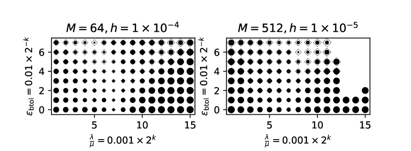
Figure 8. Performance for different $\frac{\lambda}{\mu}$ and $\varepsilon_{\rm btol}$ for the shrinking hexagon in $n=2$. The area of the discs is proportional to the logarithm of the error, while the area of the diamonds is proportional to the logarithm of the computational time. $\frac{\lambda}{\mu}=0.001\times 2^{7}\approx\frac{1}{8}$ is generally well-performing.

3.4.3. Self-similar solutions

We test the method in two and three dimensions using self-similar solutions of $V=\beta(\nu)\kappa_{\sigma}$. In two dimensions, we use the shrinking Wulff shape solution with hexagonal symmetry: the Wulff shape is the regular hexagon with edge of length $1$, Figure 9. The results are given for three different time step sizes $h$. For implementation reasons, this and the below tests with hexagonal mobility have time scaled by the factor $\frac{2\sqrt{3}}{3}$. Therefore the extinction time in $n=2$ is not $t^{*}=\frac{0.4^{2}}{2}=0.08$ as expected but $\frac{0.4^{2}\sqrt{3}}{4}\approx 0.069$, and $\frac{0.4^{2}\sqrt{3}}{8}\approx 0.035$ in $n=3$. In three dimensions, we use the shrinking Wulff shape solution when the Wulff shape is the hexagonal prism with height $2$ and regular hexagonal base with edges of length $1$, Figure 10. Finally, we use the self-similar solutions constructed in Section 2. Due to their instability, presence of different types of facets and simplicity, they seem to provide a convenient benchmark. For the crystalline shrinking doughnut, we use cubic and hexagonal anisotropies $\tilde{\sigma}$, see Figure 11 and Figure 12 respectively. The error of the sponge solution is presented in Figure 13. In all of these, the error is estimated as $\max_{m\in\mathcal{M}}\operatorname{dist}_{H,2}(\partial E(t_{m}),\partial E_{m})$ where $\mathcal{M}$ is a set of selected time steps such that for all $m\in\mathcal{M}$ we have $t_{m}=0.002z$ for some $z\in\mathbb{Z}$, and that $t_{m}$ are far enough from the extinction time $t^{*}$, where all the solutions diverge significantly due to the instability. Table 1 shows the details on the performance of the algorithm for $n=3$ and $M=64,256$.

$M=64$
	FDM		FEM
Test	#Breg/step	time/Breg (s)	#Breg/step	time/Breg (s)
Hex Wulff	$24$	$0.017$	$29$	$0.066$
$\ell^{1}$ doughnut	$35$	$0.017$	$52$	$0.068$
Hex doughnut	$38$	$0.017$	$39$	$0.075$
Sponge	$28$	$0.014$	$33$	$0.044$
$M=256$
	FDM		FEM
Test	#Breg/step	time/Breg (s)	#Breg/step	time/Breg (s)
Hex Wulff	$42$	$0.93$	$42$	$2.8$
$\ell^{1}$ doughnut	$100$	$0.68$	$109$	$3.0$
Hex doughnut	$93$	$0.78$	$98$	$3.5$
Sponge	$133$	$0.69$	$125$	$3.1$

Table 1. Performance of the numerical method in $n=3$ with $M=64$ and $M=256$ for tests in Section 3.4.3 based on the average number of Bregman iteration per time step (#Breg/step) and average time per one Bregman iterations (time/Breg (s)) in seconds. Ran on Intel Xeon CPU E5-4650 v2 @ 2.40GHz.

3.4.4. Qualitative tests

Samples of evolutions in two dimensions for various anisotropies are shown in Figure 17. In this case, the stopping condition is taken as $\left\|v_{k+1}-v_{k}\right\|_{\ell^{2}}<10^{-4}$ to illustrate the effect of choosing too large of a stopping tolerance, and therefore the very long edges in the bottom right figure are not completely straight. The stationary parts of the boundary are very well preserved and redistancing artifacts are not noticeable. In the rest of the figures, we show qualitative tests of facet breaking, bending and topological changes in $n=3$, see Figure 14, Figure 15, Figure 16 and Figure 18.

3.4.5. Discussion

The implementation of the numerical method presented in the paper is able to reproduce all of the tested features of the highly singular crystalline mean curvature flow without the need to regularize the crystalline curvature: flat faces, sharp edges and vertices, correct facet breaking and bending, and finally topological changes like neck pinching and facet-edge or edge-vertex collisions. Moreover, the method appears to be first order accurate both in space and time. We also presented a FEM discretization of the total variation energy that seems to perform visually somewhat better than the FDM discretization for non-cubic anisotropies for the cost of increased computational time. Our scheme for the reinitialization of the distance function seems to perform well without introducing redistancing artifacts.

Various optimizations, such as performing the computation only in a small neighborhood of the level set to significantly reduce the computational complexity, as well as the coupling of the curvature flow with the heat equation via the Gibbs-Thomson relation are under investigation [PozarRIMS].

Acknowledgments

Parts of this paper are based on an extended abstract for a talk that the author gave at the 2017 Spring Meeting of the Mathematical Society of Japan.

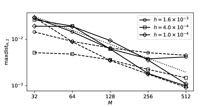
Figure 9. The error of a self-similar shrinking hexagonal Wulff shape of side-length $0.4$ in $n=2$ with the numerical solution using the FEM (solid) and FDM (dashed) discretization (maximum over $t\in[0,0.05]$). Dotted line is $M^{-1}$.

Figure 10. The error of a self-similar shrinking hexagonal Wulff shape with a hexagonal base with edges of length $0.4$ and height $0.8$ in $n=3$ with $h=10^{-4}$ as the function of $M$ (top, maximum over $t\in[0,0.026]$) and $t$ for $M=128$ (bottom).

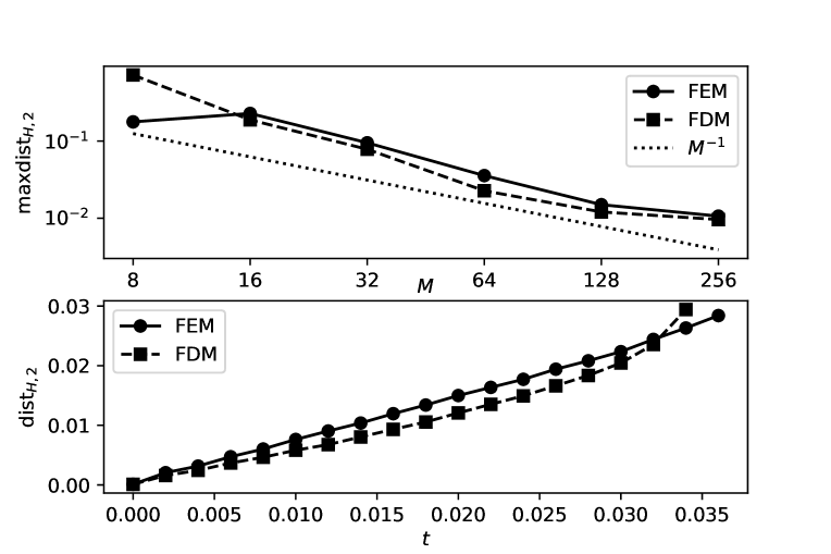
Figure 11. The error of a self-similar crystalline shrinking doughnut with $\ell^{1}$ anisotropy from Section 2.2 of side-length $0.8$ in $n=3$ with $h=10^{-4}$ as the function of $M$ (top, maximum over $t\in[0,0.02]$) and $t$ for $M=128$ (bottom).

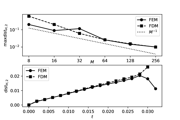
Figure 12. The error of a self-similar crystalline shrinking doughnut with hexagonal anisotropy from Section 2.2 of hexagonal base with side-length $0.4$ and height $0.8$ in $n=3$ with $h=10^{-4}$ as the function of $M$ (top, maximum over $t\in[0,0.02]$) and $t$ for $M=128$ (bottom).

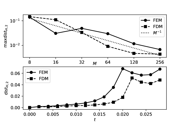
Figure 13. The error of a self-similar shrinking sponge from Section 2.3 with $R_{0}=0.4$ in $n=3$ with $h=10^{-4}$ as the function of $M$ (top, maximum over $t\in[0,0.014]$) and $t$ for $M=128$ (bottom).

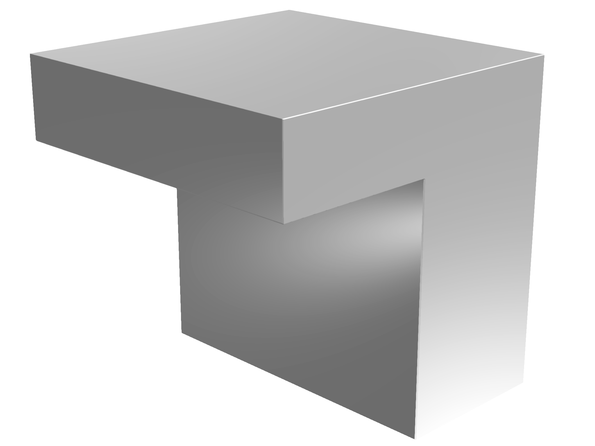
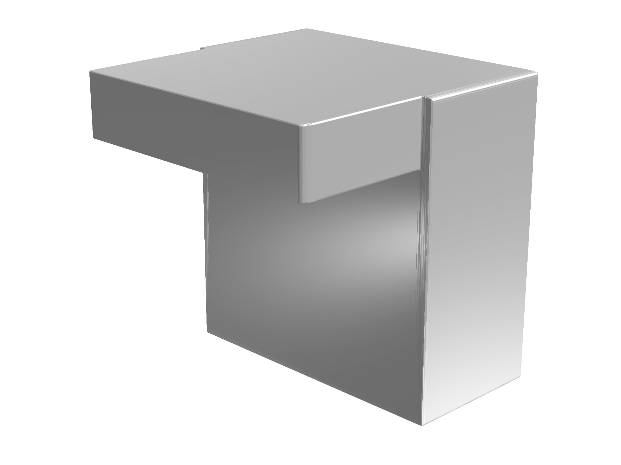
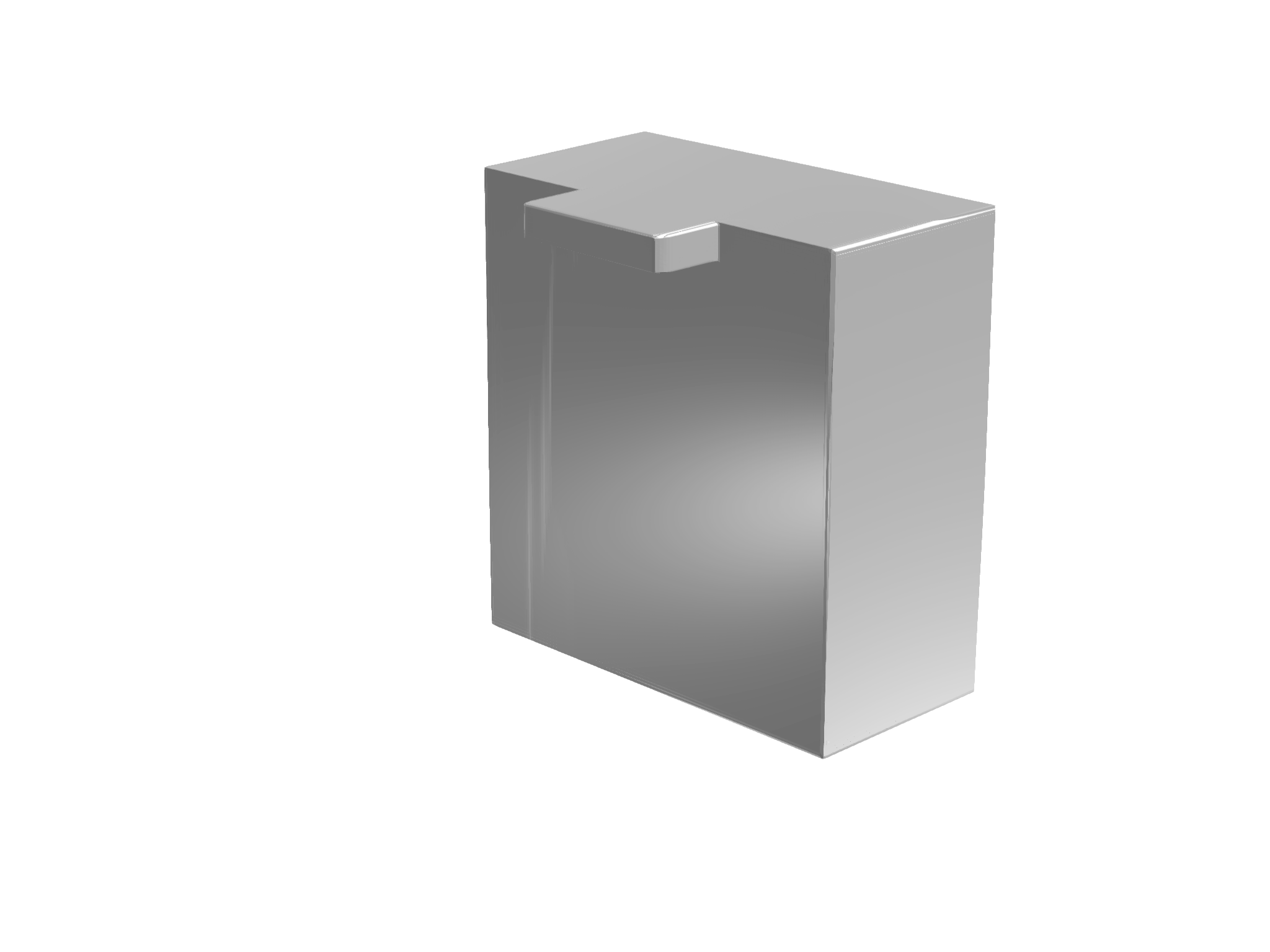
Figure 14. Facet breaking example in 3D [BNP99] at three selected times—L-shaped facets break into rectangular facets.

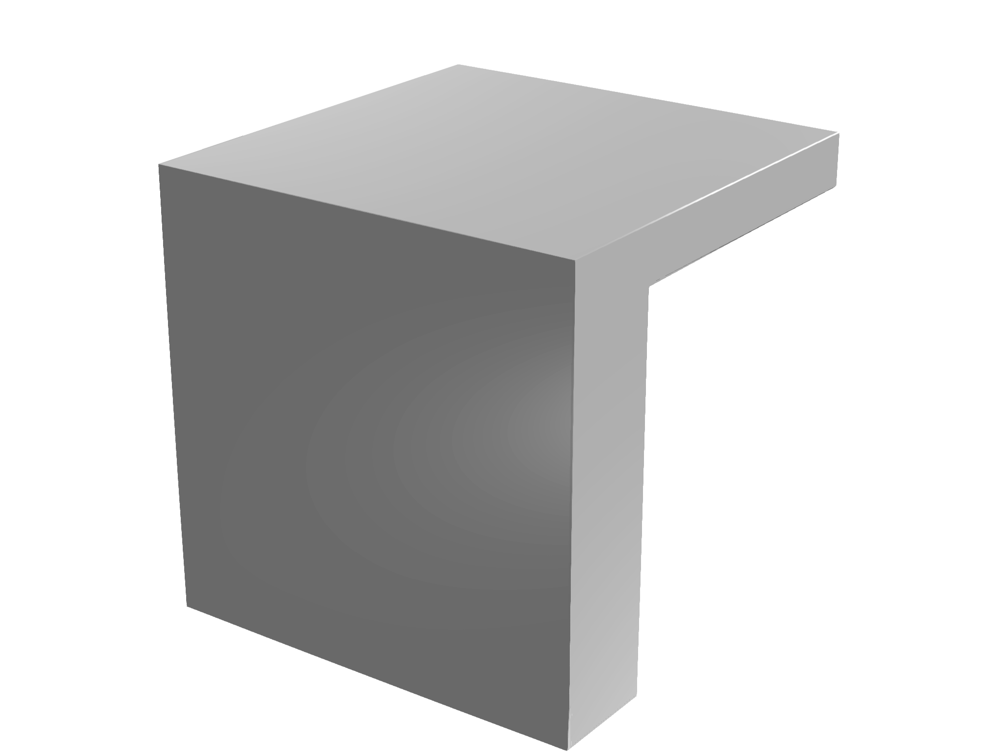
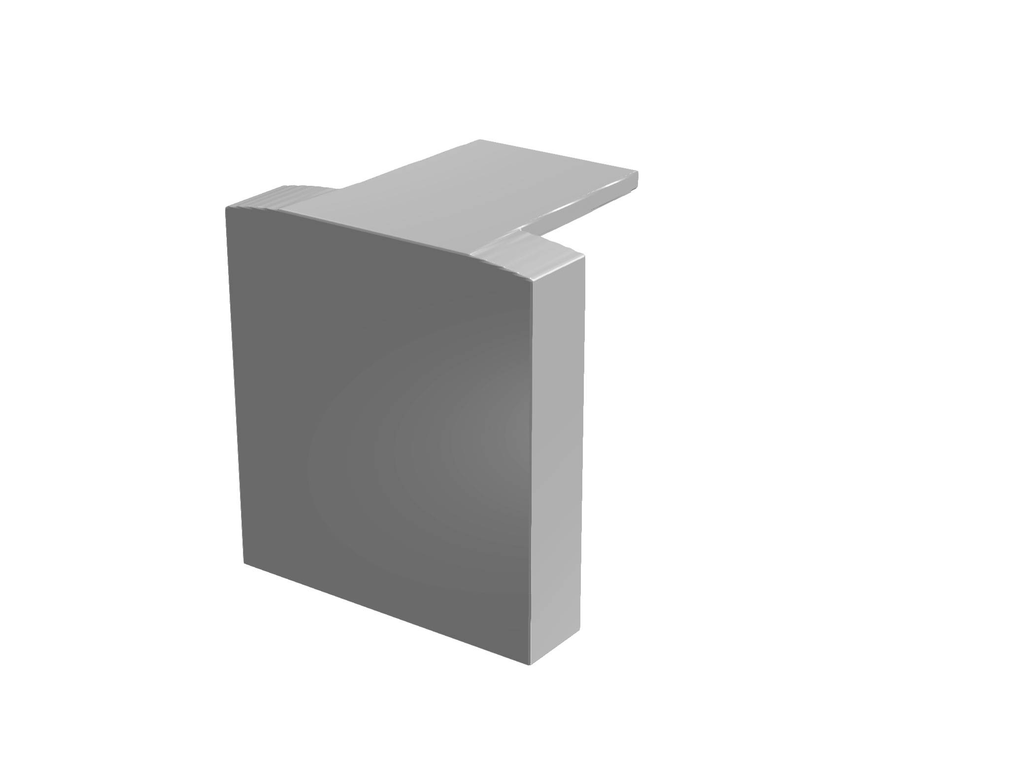
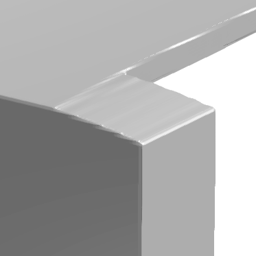
Figure 15. Facet bending (the top facet) in an axes-aligned initial shape for the cubic ($\ell^{1}$) anisotropy [Lasica-comm], with a detail on the right.

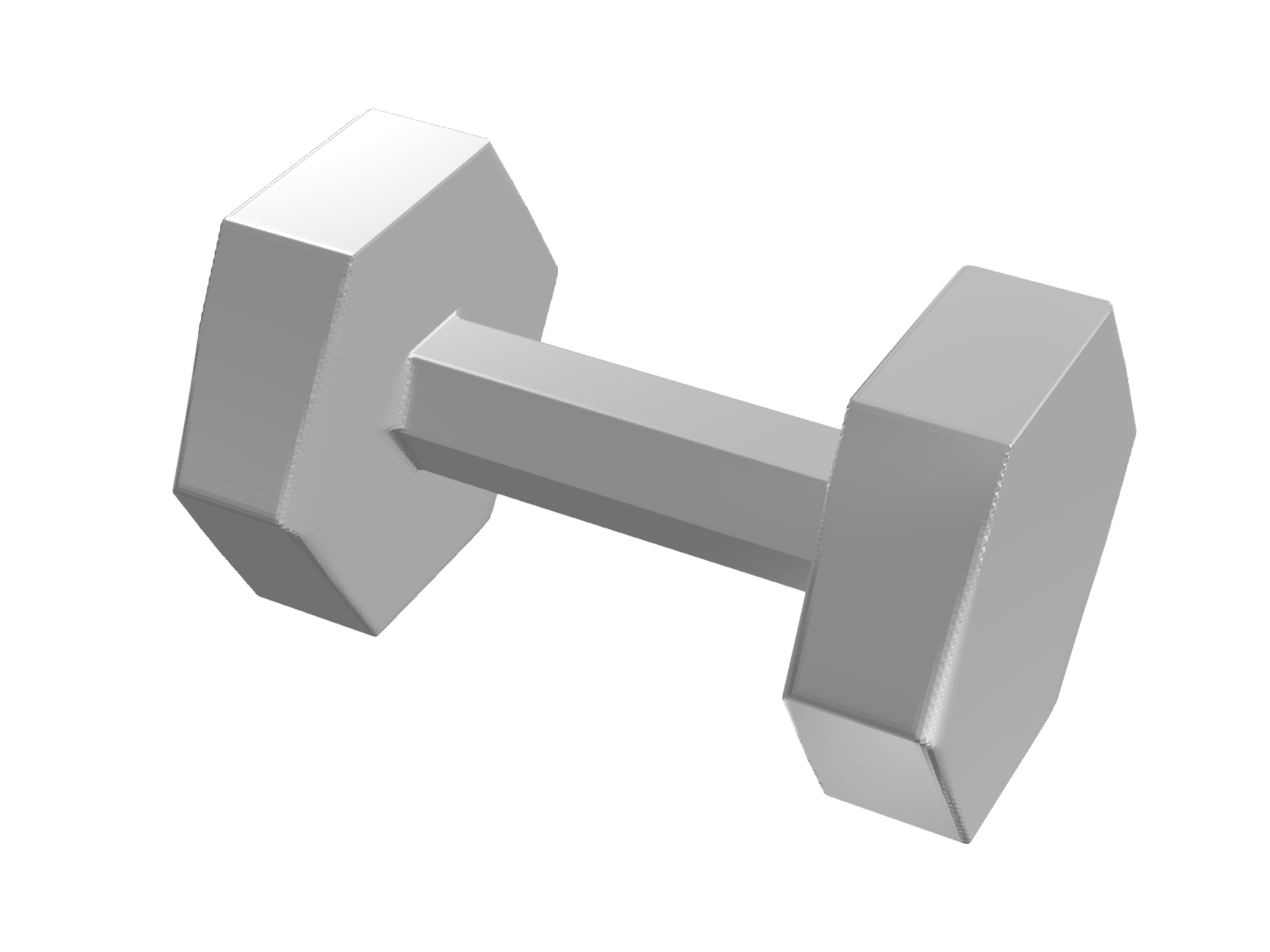
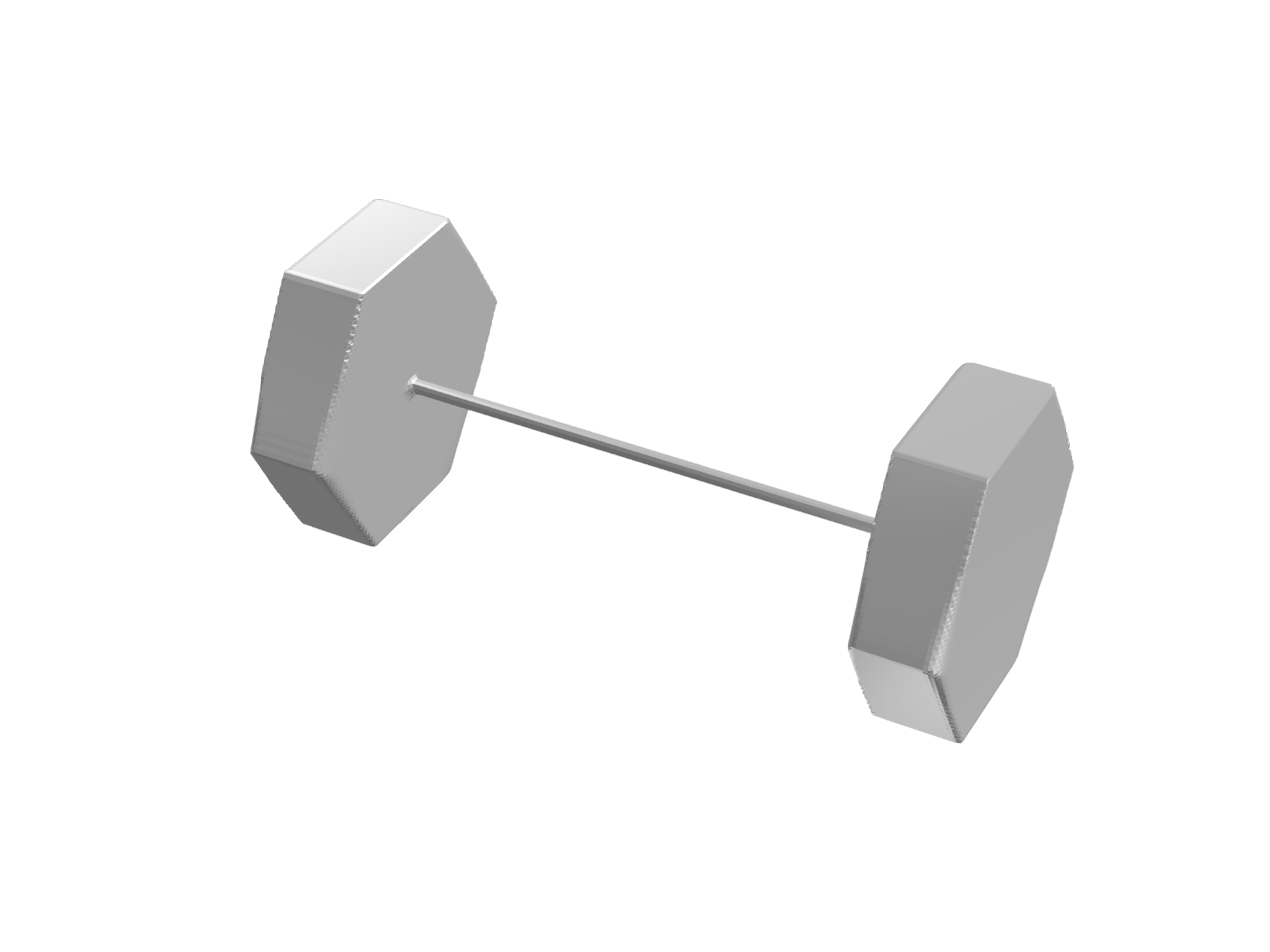
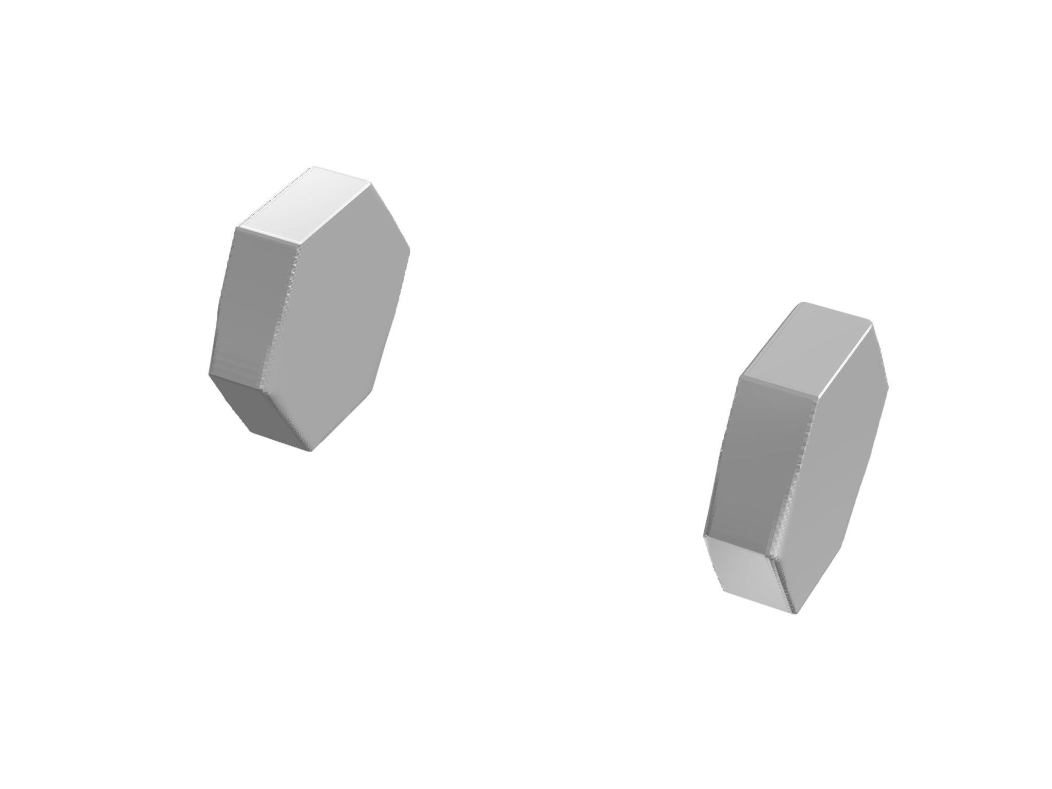
Figure 16. Topological change in 3D with a hexagonal anisotropy—a pinch-off of an initially connected dumbbell shape. FDM discretization; some rounding of edges is apparent.

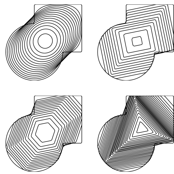
Figure 17. Flow $V=\kappa_{\sigma}$ with various anisotropies: $h=10^{-4}$, $M=64$, FEM discretization and plot step $0.005=50h$. The bounding box of the initial curve is the square $[-0.4,0.4]^{2}$ inside the computational domain $(-\frac{1}{2},\frac{1}{2})^{2}$. Even at this relatively low resolution, artifacts caused by the redistance are not apparent.

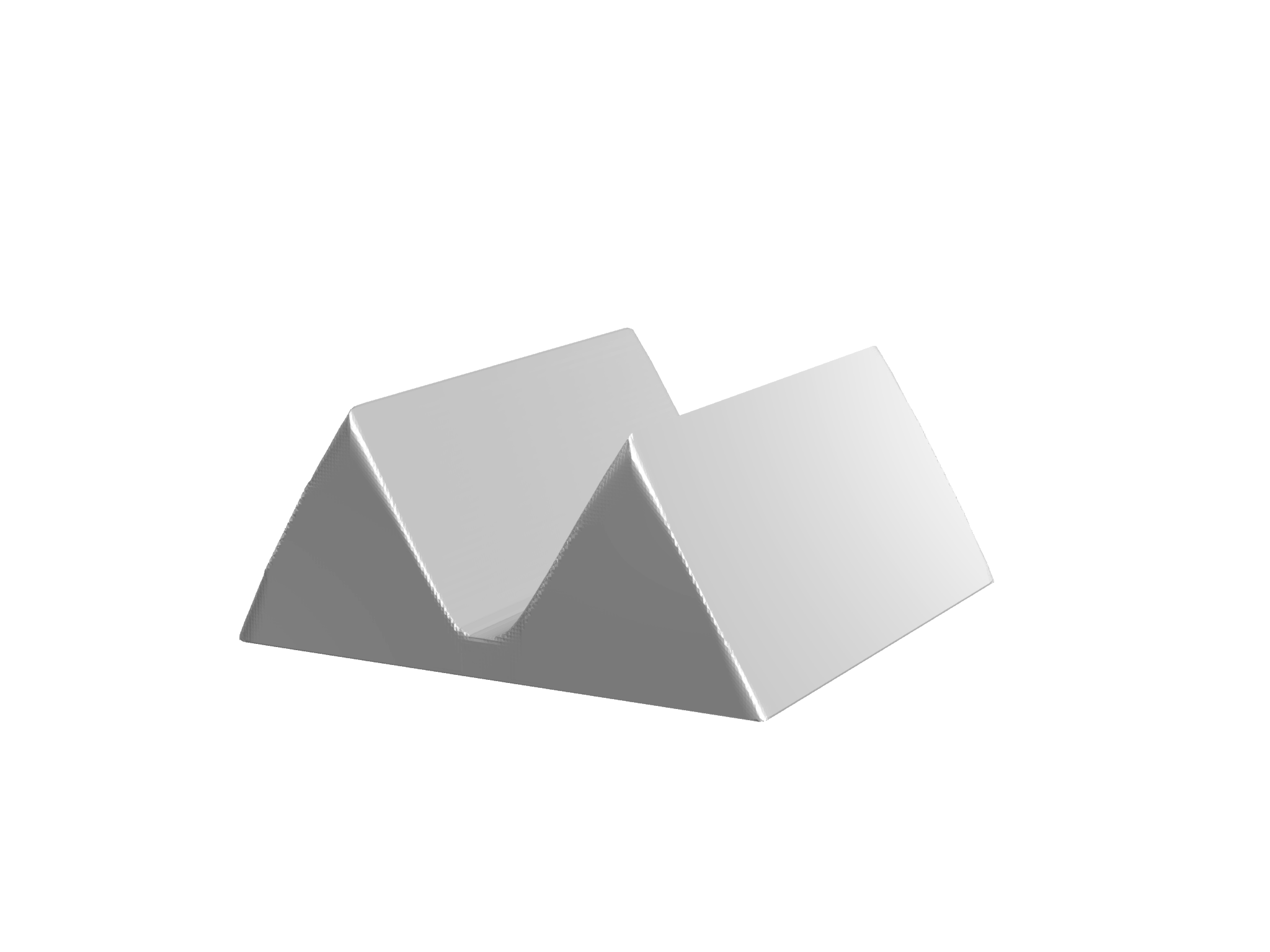
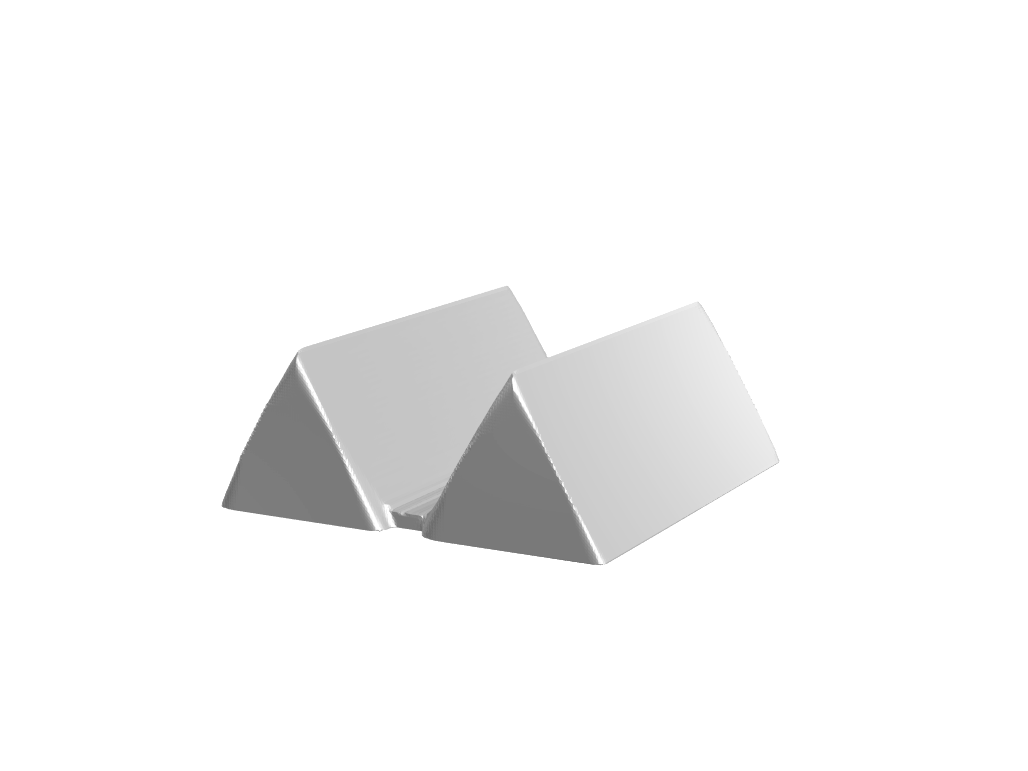
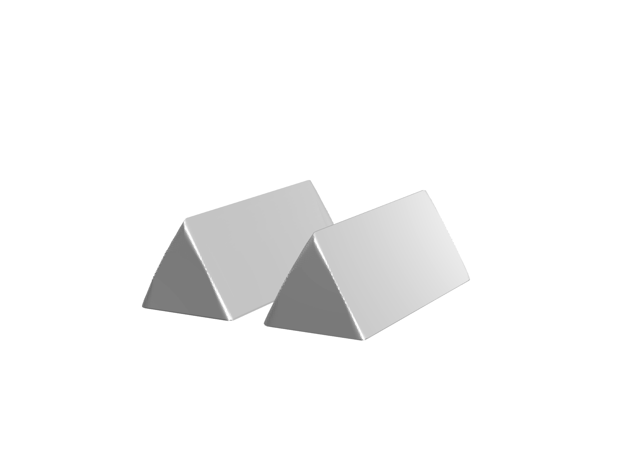
Figure 18. Topological change in 3D with a triangular anisotropy—a pinch-off due to a collision of a facet and an edge. FEM discretization.

References

AdalsteinssonD.SethianJ. A.The fast construction of extension velocities in level set methodsJ. Comput. Phys.148199912–22ISSN 0021-9991Document@article{AS, author = {Adalsteinsson, D.}, author = {Sethian, J. A.}, title = {The fast construction of extension velocities in level set methods}, journal = {J. Comput. Phys.}, volume = {148}, date = {1999}, number = {1}, pages = {2–22}, issn = {0021-9991}, doi = {10.1006/jcph.1998.6090}} AlmgrenFredTaylorJean E.WangLiheCurvature-driven flows: a variational approachSIAM J. Control Optim.3119932387–438ISSN 0363-0129Document@article{ATW, author = {Almgren, Fred}, author = {Taylor, Jean E.}, author = {Wang, Lihe}, title = {Curvature-driven flows: a variational approach}, journal = {SIAM J. Control Optim.}, volume = {31}, date = {1993}, number = {2}, pages = {387–438}, issn = {0363-0129}, doi = {10.1137/0331020}} Andreu-VailloFuensantaCasellesVicentMazónJosé M.Parabolic quasilinear equations minimizing linear growth functionalsProgress in Mathematics223Birkhäuser VerlagBasel2004xiv+340ISBN 3-7643-6619-2Review MathReviews@book{ACM, author = {Andreu-Vaillo, Fuensanta}, author = {Caselles, Vicent}, author = {Maz{\'o}n, Jos{\'e} M.}, title = {Parabolic quasilinear equations minimizing linear growth functionals}, series = {Progress in Mathematics}, volume = {223}, publisher = {Birkh\"auser Verlag}, place = {Basel}, date = {2004}, pages = {xiv+340}, isbn = {3-7643-6619-2}, review = {\MR{2033382 (2005c:35002)}}} AngenentSigurd B.Shrinking doughnutstitle={Nonlinear diffusion equations and their equilibrium states, 3}, address={Gregynog}, date={1989}, series={Progr. Nonlinear Differential Equations Appl.}, volume={7}, publisher={Birkh\"auser Boston, Boston, MA}, 199221–38Review MathReviews@article{Angenent, author = {Angenent, Sigurd B.}, title = {Shrinking doughnuts}, conference = {title={Nonlinear diffusion equations and their equilibrium states, 3}, address={Gregynog}, date={1989}, }, book = {series={Progr. Nonlinear Differential Equations Appl.}, volume={7}, publisher={Birkh\"auser Boston, Boston, MA}, }, date = {1992}, pages = {21–38}, review = {\MR{1167827}}} AngenentSigurdGurtinMorton E.Multiphase thermomechanics with interfacial structure. ii. evolution of an isothermal interfaceArch. Rational Mech. Anal.10819894323–391ISSN 0003-9527Document@article{AG89, author = {Angenent, Sigurd}, author = {Gurtin, Morton E.}, title = {Multiphase thermomechanics with interfacial structure. II.\ Evolution of an isothermal interface}, journal = {Arch. Rational Mech. Anal.}, volume = {108}, date = {1989}, number = {4}, pages = {323–391}, issn = {0003-9527}, doi = {10.1007/BF01041068}} BarrettJohn W.GarckeHaraldNürnbergRobertA variational formulation of anisotropic geometric evolution equations in higher dimensionsNumer. Math.109200811–44ISSN 0029-599XReview MathReviewsDocument@article{BGN_NM, author = {Barrett, John W.}, author = {Garcke, Harald}, author = {N\"urnberg, Robert}, title = {A variational formulation of anisotropic geometric evolution equations in higher dimensions}, journal = {Numer. Math.}, volume = {109}, date = {2008}, number = {1}, pages = {1–44}, issn = {0029-599X}, review = {\MR{2377611}}, doi = {10.1007/s00211-007-0135-5}} BarrettJohn W.GarckeHaraldNürnbergRobertParametric approximation of surface clusters driven by isotropic and anisotropic surface energiesInterfaces Free Bound.1220102187–234ISSN 1463-9963Review MathReviewsDocument@article{BGN_IFB, author = {Barrett, John W.}, author = {Garcke, Harald}, author = {N\"urnberg, Robert}, title = {Parametric approximation of surface clusters driven by isotropic and anisotropic surface energies}, journal = {Interfaces Free Bound.}, volume = {12}, date = {2010}, number = {2}, pages = {187–234}, issn = {1463-9963}, review = {\MR{2652017}}, doi = {10.4171/IFB/232}} BarrettJohn W.GarckeHaraldNürnbergRobertFinite-element approximation of one-sided stefan problems with anisotropic, approximately crystalline, gibbs-thomson lawAdv. Differential Equations1820133-4383–432ISSN 1079-9389@article{BGN, author = {Barrett, John W.}, author = {Garcke, Harald}, author = {N\"urnberg, Robert}, title = {Finite-element approximation of one-sided Stefan problems with anisotropic, approximately crystalline, Gibbs-Thomson law}, journal = {Adv. Differential Equations}, volume = {18}, date = {2013}, number = {3-4}, pages = {383–432}, issn = {1079-9389}} BarrettJohn W.GarckeHaraldNürnbergRobertOn the stable discretization of strongly anisotropic phase field models with applications to crystal growthZAMM Z. Angew. Math. Mech.93201310-11719–732ISSN 0044-2267Review MathReviewsDocument@article{BGN_ZAMM, author = {Barrett, John W.}, author = {Garcke, Harald}, author = {N\"urnberg, Robert}, title = {On the stable discretization of strongly anisotropic phase field models with applications to crystal growth}, journal = {ZAMM Z. Angew. Math. Mech.}, volume = {93}, date = {2013}, number = {10-11}, pages = {719–732}, issn = {0044-2267}, review = {\MR{3118772}}, doi = {10.1002/zamm.201200147}} BarrettJohn W.GarckeHaraldNürnbergRobertStable phase field approximations of anisotropic solidificationIMA J. Numer. Anal.34201441289–1327ISSN 0272-4979Review MathReviewsDocument@article{BGN_IMA, author = {Barrett, John W.}, author = {Garcke, Harald}, author = {N\"urnberg, Robert}, title = {Stable phase field approximations of anisotropic solidification}, journal = {IMA J. Numer. Anal.}, volume = {34}, date = {2014}, number = {4}, pages = {1289–1327}, issn = {0272-4979}, review = {\MR{3269427}}, doi = {10.1093/imanum/drt044}} BellettiniG.An introduction to anisotropic and crystalline mean curvature flowHokkaido Univ. Tech. Rep. Ser. in Math.1452010102–162@article{B10, author = {Bellettini, G.}, title = {An introduction to anisotropic and crystalline mean curvature flow}, journal = {Hokkaido Univ. Tech. Rep. Ser. in Math.}, volume = {145}, date = {2010}, pages = {102–162}} BellettiniGiovanniCasellesVicentChambolleAntoninNovagaMatteoCrystalline mean curvature flow of convex setsArch. Ration. Mech. Anal.17920061109–152ISSN 0003-9527Document@article{BCCN06, author = {Bellettini, Giovanni}, author = {Caselles, Vicent}, author = {Chambolle, Antonin}, author = {Novaga, Matteo}, title = {Crystalline mean curvature flow of convex sets}, journal = {Arch. Ration. Mech. Anal.}, volume = {179}, date = {2006}, number = {1}, pages = {109–152}, issn = {0003-9527}, doi = {10.1007/s00205-005-0387-0}} BellettiniG.NovagaM.Approximation and comparison for nonsmooth anisotropic motion by mean curvature in ${\bf R}^{N}$Math. Models Methods Appl. Sci.10200011–10ISSN 0218-2025Document@article{BN00, author = {Bellettini, G.}, author = {Novaga, M.}, title = {Approximation and comparison for nonsmooth anisotropic motion by mean curvature in ${\bf R}^N$}, journal = {Math. Models Methods Appl. Sci.}, volume = {10}, date = {2000}, number = {1}, pages = {1–10}, issn = {0218-2025}, doi = {10.1142/S0218202500000021}} BellettiniG.NovagaM.PaoliniM.Facet-breaking for three-dimensional crystals evolving by mean curvatureInterfaces Free Bound.11999139–55ISSN 1463-9963Document@article{BNP99, author = {Bellettini, G.}, author = {Novaga, M.}, author = {Paolini, M.}, title = {Facet-breaking for three-dimensional crystals evolving by mean curvature}, journal = {Interfaces Free Bound.}, volume = {1}, date = {1999}, number = {1}, pages = {39–55}, issn = {1463-9963}, doi = {10.4171/IFB/3}} BellettiniG.NovagaM.PaoliniM.On a crystalline variational problem. i. first variation and global $L^{\infty}$ regularityArch. Ration. Mech. Anal.15720013165–191ISSN 0003-9527Document@article{BNP01a, author = {Bellettini, G.}, author = {Novaga, M.}, author = {Paolini, M.}, title = {On a crystalline variational problem. I. First variation and global $L^\infty$ regularity}, journal = {Arch. Ration. Mech. Anal.}, volume = {157}, date = {2001}, number = {3}, pages = {165–191}, issn = {0003-9527}, doi = {10.1007/s002050010127}} BrézisHaïmMonotonicity methods in hilbert spaces and some applications to nonlinear partial differential equationstitle={Contributions to nonlinear functional analysis}, address={Proc. Sympos., Math. Res. Center, Univ. Wisconsin, Madison, Wis.}, date={1971}, publisher={Academic Press, New York}, 1971101–156@article{Br71, author = {Br{\'e}zis, Ha{\"{\i}}m}, title = {Monotonicity methods in Hilbert spaces and some applications to nonlinear partial differential equations}, conference = {title={Contributions to nonlinear functional analysis}, address={Proc. Sympos., Math. Res. Center, Univ. Wisconsin, Madison, Wis.}, date={1971}, }, book = {publisher={Academic Press, New York}, }, date = {1971}, pages = {101–156}} ChambolleAntoninAn algorithm for mean curvature motionInterfaces Free Bound.620042195–218ISSN 1463-9963Document@article{Chambolle, author = {Chambolle, Antonin}, title = {An algorithm for mean curvature motion}, journal = {Interfaces Free Bound.}, volume = {6}, date = {2004}, number = {2}, pages = {195–218}, issn = {1463-9963}, doi = {10.4171/IFB/97}} ChambolleAntoninMoriniMassimilianoNovagaMatteoPonsiglioneMarcelloExistence and uniqueness for anisotropic and crystalline mean curvature flowshttps://arxiv.org/abs/1702.03094preprint@article{CMNP, author = {Chambolle, Antonin}, author = {Morini, Massimiliano}, author = {Novaga, Matteo}, author = {Ponsiglione, Marcello}, title = {Existence and uniqueness for anisotropic and crystalline mean curvature flows}, eprint = {https://arxiv.org/abs/1702.03094}, status = {preprint}} ChambolleAntoninMoriniMassimilianoPonsiglioneMarcelloExistence and uniqueness for a crystalline mean curvature flowComm. Pure Appl. Math.70201761084–1114ISSN 0010-3640Review MathReviewsDocument@article{CMP, author = {Chambolle, Antonin}, author = {Morini, Massimiliano}, author = {Ponsiglione, Marcello}, title = {Existence and uniqueness for a crystalline mean curvature flow}, journal = {Comm. Pure Appl. Math.}, volume = {70}, date = {2017}, number = {6}, pages = {1084–1114}, issn = {0010-3640}, review = {\MR{3639320}}, doi = {10.1002/cpa.21668}} ChenYun GangGigaYoshikazuGotoShun’ichiUniqueness and existence of viscosity solutions of generalized mean curvature flow equationsJ. Differential Geom.3319913749–786ISSN 0022-040X@article{CGG, author = {Chen, Yun Gang}, author = {Giga, Yoshikazu}, author = {Goto, Shun'ichi}, title = {Uniqueness and existence of viscosity solutions of generalized mean curvature flow equations}, journal = {J. Differential Geom.}, volume = {33}, date = {1991}, number = {3}, pages = {749–786}, issn = {0022-040X}} ChoppDavid L.Experiment. Math.11–15A K Peters, Ltd.Computation of self-similar solutions for mean curvature flow31994@article{Chopp, author = {Chopp, David L.}, journal = {Experiment. Math.}, number = {1}, pages = {1–15}, publisher = {A K Peters, Ltd.}, title = {Computation of self-similar solutions for mean curvature flow}, volume = {3}, year = {1994}} An efficient method of triangulating equi-valued surfaces by using tetrahedral cellsDoiAkioKoideAkioIEICE TRANSACTIONS on Information and SystemsE74-D1214–2241991@article{DK, title = {An Efficient Method of Triangulating Equi-Valued Surfaces by Using Tetrahedral Cells}, author = {Doi, Akio}, author = {Koide, Akio}, journal = {IEICE TRANSACTIONS on Information and Systems}, volume = {E74-D}, number = {1}, pages = {214–224}, date = {1991}} EvansL. C.SpruckJ.Motion of level sets by mean curvature. iJ. Differential Geom.3319913635–681ISSN 0022-040X@article{ES, author = {Evans, L. C.}, author = {Spruck, J.}, title = {Motion of level sets by mean curvature. I}, journal = {J. Differential Geom.}, volume = {33}, date = {1991}, number = {3}, pages = {635–681}, issn = {0022-040X}} GageM.HamiltonR. S.The heat equation shrinking convex plane curvesJ. Differential Geom.231986169–96ISSN 0022-040XReview MathReviews@article{GageHamilton, author = {Gage, M.}, author = {Hamilton, R. S.}, title = {The heat equation shrinking convex plane curves}, journal = {J. Differential Geom.}, volume = {23}, date = {1986}, number = {1}, pages = {69–96}, issn = {0022-040X}, review = {\MR{840401}}} GarckeHaraldCurvature driven interface evolutionJahresber. Dtsch. Math.-Ver.1152013263–100ISSN 0012-0456Document@article{GarckeSurvey, author = {Garcke, Harald}, title = {Curvature driven interface evolution}, journal = {Jahresber. Dtsch. Math.-Ver.}, volume = {115}, date = {2013}, number = {2}, pages = {63–100}, issn = {0012-0456}, doi = {10.1365/s13291-013-0066-2}} GigaYoshikazuSurface evolution equations - a level set approachMonographs in Mathematics99(earlier version: Lipschitz Lecture Notes 44, University of Bonn, 2002)Birkhäuser Verlag, Basel2006xii+264ISBN 978-3-7643-2430-8ISBN 3-7643-2430-9@book{G06, author = {Giga, Yoshikazu}, title = {Surface evolution equations - a level set approach}, series = {Monographs in Mathematics}, volume = {99}, note = {(earlier version: Lipschitz Lecture Notes \textbf{44}, University of Bonn, 2002)}, publisher = {Birkh\"auser Verlag, Basel}, date = {2006}, pages = {xii+264}, isbn = {978-3-7643-2430-8}, isbn = {3-7643-2430-9}} GigaMi-HoGigaYoshikazuEvolving graphs by singular weighted curvatureArch. Rational Mech. Anal.14119982117–198ISSN 0003-9527@article{GG98ARMA, author = {Giga, Mi-Ho}, author = {Giga, Yoshikazu}, title = {Evolving graphs by singular weighted curvature}, journal = {Arch. Rational Mech. Anal.}, volume = {141}, date = {1998}, number = {2}, pages = {117–198}, issn = {0003-9527}} GigaMi-HoGigaYoshikazuCrystalline and level set flow—convergence of a crystalline algorithm for a general anisotropic curvature flow in the planetitle={Free boundary problems: theory and applications, I}, address={Chiba}, date={1999}, series={GAKUTO Internat. Ser. Math. Sci. Appl.}, volume={13}, publisher={Gakk\=otosho, Tokyo}, 200064–79Review MathReviews@article{GGGakuto, author = {Giga, Mi-Ho}, author = {Giga, Yoshikazu}, title = {Crystalline and level set flow—convergence of a crystalline algorithm for a general anisotropic curvature flow in the plane}, conference = {title={Free boundary problems: theory and applications, I}, address={Chiba}, date={1999}, }, book = {series={GAKUTO Internat. Ser. Math. Sci. Appl.}, volume={13}, publisher={Gakk\=otosho, Tokyo}, }, date = {2000}, pages = {64–79}, review = {\MR{1793023}}} GigaMi-HoGigaYoshikazuGeneralized motion by nonlocal curvature in the planeArch. Ration. Mech. Anal.15920014295–333ISSN 0003-9527Document@article{GG01, author = {Giga, Mi-Ho}, author = {Giga, Yoshikazu}, title = {Generalized motion by nonlocal curvature in the plane}, journal = {Arch. Ration. Mech. Anal.}, volume = {159}, date = {2001}, number = {4}, pages = {295–333}, issn = {0003-9527}, doi = {10.1007/s002050100154}} GigaMi-HoGigaYoshikazuHontaniHidekataSelf-similar expanding solutions in a sector for a crystalline flowSIAM J. Math. Anal.37200541207–1226ISSN 0036-1410Review MathReviewsDocument@article{GGH, author = {Giga, Mi-Ho}, author = {Giga, Yoshikazu}, author = {Hontani, Hidekata}, title = {Self-similar expanding solutions in a sector for a crystalline flow}, journal = {SIAM J. Math. Anal.}, volume = {37}, date = {2005}, number = {4}, pages = {1207–1226}, issn = {0036-1410}, review = {\MR{2192293}}, doi = {10.1137/040614372}} GigaM.-H.GigaY.RybkaP.A comparison principle for singular diffusion equations with spatially inhomogeneous driving force for graphsArch. Ration. Mech. Anal.21120142419–453ISSN 0003-9527Document@article{GGR, author = {Giga, M.-H.}, author = {Giga, Y.}, author = {Rybka, P.}, title = {A comparison principle for singular diffusion equations with spatially inhomogeneous driving force for graphs}, journal = {Arch. Ration. Mech. Anal.}, volume = {211}, date = {2014}, number = {2}, pages = {419–453}, issn = {0003-9527}, doi = {10.1007/s00205-013-0676-y}} GigaYoshikazuGórkaPrzemysławRybkaPiotrBent rectangles as viscosity solutions over a circleNonlinear Anal.1252015518–549ISSN 0362-546XDocument@article{GGR15, author = {Giga, Yoshikazu}, author = {G\'orka, Przemys\l aw}, author = {Rybka, Piotr}, title = {Bent rectangles as viscosity solutions over a circle}, journal = {Nonlinear Anal.}, volume = {125}, date = {2015}, pages = {518–549}, issn = {0362-546X}, doi = {10.1016/j.na.2015.05.033}} GigaYoshikazuPožárNorbertA level set crystalline mean curvature flow of surfacesAdv. Differential Equations2120167-8631–698ISSN 1079-9389@article{GP16, author = {Giga, Yoshikazu}, author = {Po{\v{z}}{\'a}r, Norbert}, title = {A level set crystalline mean curvature flow of surfaces}, journal = {Adv. Differential Equations}, volume = {21}, date = {2016}, number = {7-8}, pages = {631–698}, issn = {1079-9389}} GigaYoshikazuPožárNorbertApproximation of general facets by admissible facets for anisotropic total variation energies and its application to the crystalline mean curvature flowComm. Pure Appl. Math.71201871461–1491Document@article{GP_CPAM, author = {Giga, Yoshikazu}, author = {Po{\v{z}}{\'a}r, Norbert}, title = {Approximation of general facets by admissible facets for anisotropic total variation energies and its application to the crystalline mean curvature flow}, journal = {Comm. Pure Appl. Math.}, volume = {71}, date = {2018}, number = {7}, pages = {1461–1491}, doi = {doi.org/10.1002/cpa.21752}} GoldsteinTomOsherStanleyThe split bregman method for $L1$-regularized problemsSIAM J. Imaging Sci.220092323–343ISSN 1936-4954Document@article{GO, author = {Goldstein, Tom}, author = {Osher, Stanley}, title = {The split Bregman method for $L1$-regularized problems}, journal = {SIAM J. Imaging Sci.}, volume = {2}, date = {2009}, number = {2}, pages = {323–343}, issn = {1936-4954}, doi = {10.1137/080725891}} GraysonMatthew A.The heat equation shrinks embedded plane curves to round pointsJ. Differential Geom.2619872285–314ISSN 0022-040XReview MathReviews@article{Grayson, author = {Grayson, Matthew A.}, title = {The heat equation shrinks embedded plane curves to round points}, journal = {J. Differential Geom.}, volume = {26}, date = {1987}, number = {2}, pages = {285–314}, issn = {0022-040X}, review = {\MR{906392}}} GurtinMorton E.Thermomechanics of evolving phase boundaries in the planeOxford Mathematical MonographsThe Clarendon Press, Oxford University Press, New York1993xi+148ISBN 0-19-853694-1@book{Gurtin, author = {Gurtin, Morton E.}, title = {Thermomechanics of evolving phase boundaries in the plane}, series = {Oxford Mathematical Monographs}, publisher = {The Clarendon Press, Oxford University Press, New York}, date = {1993}, pages = {xi+148}, isbn = {0-19-853694-1}} HuiskenGerhardFlow by mean curvature of convex surfaces into spheresJ. Differential Geom.2019841237–266ISSN 0022-040XReview MathReviews@article{Huisken, author = {Huisken, Gerhard}, title = {Flow by mean curvature of convex surfaces into spheres}, journal = {J. Differential Geom.}, volume = {20}, date = {1984}, number = {1}, pages = {237–266}, issn = {0022-040X}, review = {\MR{772132}}} IshiiKatsuyukiAn approximation scheme for the anisotropic and nonlocal mean curvature flowNoDEA Nonlinear Differential Equations Appl.2120142219–252ISSN 1021-9722Document@article{Ishii14, author = {Ishii, Katsuyuki}, title = {An approximation scheme for the anisotropic and nonlocal mean curvature flow}, journal = {NoDEA Nonlinear Differential Equations Appl.}, volume = {21}, date = {2014}, number = {2}, pages = {219–252}, issn = {1021-9722}, doi = {10.1007/s00030-013-0244-z}} IshiwataTetsuyaUshijimaTakeo K.YagisitaHirokiYazakiShigetoshiTwo examples of nonconvex self-similar solution curves for a crystalline curvature flowProc. Japan Acad. Ser. A Math. Sci.8020048151–154ISSN 0386-2194Review MathReviews@article{IUYY, author = {Ishiwata, Tetsuya}, author = {Ushijima, Takeo K.}, author = {Yagisita, Hiroki}, author = {Yazaki, Shigetoshi}, title = {Two examples of nonconvex self-similar solution curves for a crystalline curvature flow}, journal = {Proc. Japan Acad. Ser. A Math. Sci.}, volume = {80}, date = {2004}, number = {8}, pages = {151–154}, issn = {0386-2194}, review = {\MR{2099341}}} KōmuraYukioNonlinear semi-groups in hilbert spaceJ. Math. Soc. Japan191967493–507ISSN 0025-5645@article{Komura67, author = {K{\=o}mura, Yukio}, title = {Nonlinear semi-groups in Hilbert space}, journal = {J. Math. Soc. Japan}, volume = {19}, date = {1967}, pages = {493–507}, issn = {0025-5645}} ŁasicaMichalPersonal communication2016@article{Lasica-comm, author = {\L asica, Michal}, title = {Personal communication}, date = {2016}} ŁasicaMichałMollSalvadorMuchaPiotr B.Total variation denoising in $l^{1}$ anisotropySIAM J. Imaging Sci.10201741691–1723ISSN 1936-4954Review MathReviews@article{LMM, author = {\L asica, Micha\l}, author = {Moll, Salvador}, author = {Mucha, Piotr B.}, title = {Total Variation Denoising in $l^1$ Anisotropy}, journal = {SIAM J. Imaging Sci.}, volume = {10}, date = {2017}, number = {4}, pages = {1691–1723}, issn = {1936-4954}, review = {\MR{3709886}}} NguyenXuan HienConstruction of complete embedded self-similar surfaces under mean curvature flow. iTrans. Amer. Math. Soc.361200941683–1701ISSN 0002-9947Review MathReviewsDocument@article{Nguyen_TransAMS, author = {Nguyen, Xuan Hien}, title = {Construction of complete embedded self-similar surfaces under mean curvature flow. I}, journal = {Trans. Amer. Math. Soc.}, volume = {361}, date = {2009}, number = {4}, pages = {1683–1701}, issn = {0002-9947}, review = {\MR{2465812}}, doi = {10.1090/S0002-9947-08-04748-X}} NguyenXuan HienConstruction of complete embedded self-similar surfaces under mean curvature flow. iiAdv. Differential Equations1520105-6503–530ISSN 1079-9389Review MathReviews@article{Nguyen_ADE, author = {Nguyen, Xuan Hien}, title = {Construction of complete embedded self-similar surfaces under mean curvature flow. II}, journal = {Adv. Differential Equations}, volume = {15}, date = {2010}, number = {5-6}, pages = {503–530}, issn = {1079-9389}, review = {\MR{2643233}}} NguyenXuan HienConstruction of complete embedded self-similar surfaces under mean curvature flow, part iiiDuke Math. J.1632014112023–2056ISSN 0012-7094Review MathReviewsDocument@article{Nguyen_Duke, author = {Nguyen, Xuan Hien}, title = {Construction of complete embedded self-similar surfaces under mean curvature flow, Part III}, journal = {Duke Math. J.}, volume = {163}, date = {2014}, number = {11}, pages = {2023–2056}, issn = {0012-7094}, review = {\MR{3263027}}, doi = {10.1215/00127094-2795108}} NovagaMatteoPaoliniEmanueleStability of crystalline evolutionsMath. Models Methods Appl. Sci.1520056921–937ISSN 0218-2025Review MathReviewsDocument@article{NP_MMMAS, author = {Novaga, Matteo}, author = {Paolini, Emanuele}, title = {Stability of crystalline evolutions}, journal = {Math. Models Methods Appl. Sci.}, volume = {15}, date = {2005}, number = {6}, pages = {921–937}, issn = {0218-2025}, review = {\MR{2149929}}, doi = {10.1142/S0218202505000571}} ObermanAdamOsherStanleyTakeiRyoTsaiRichardNumerical methods for anisotropic mean curvature flow based on a discrete time variational formulationCommun. Math. Sci.920113637–662ISSN 1539-6746Document@article{OOTT, author = {Oberman, Adam}, author = {Osher, Stanley}, author = {Takei, Ryo}, author = {Tsai, Richard}, title = {Numerical methods for anisotropic mean curvature flow based on a discrete time variational formulation}, journal = {Commun. Math. Sci.}, volume = {9}, date = {2011}, number = {3}, pages = {637–662}, issn = {1539-6746}, doi = {10.4310/CMS.2011.v9.n3.a1}} OsherStanleySethianJames A.Fronts propagating with curvature-dependent speed: algorithms based on hamilton-jacobi formulationsJ. Comput. Phys.791988no. 112–49ISSN 0021-9991@article{OS, author = {Osher, Stanley}, author = {Sethian, James A.}, title = {Fronts propagating with curvature-dependent speed: algorithms based on Hamilton-Jacobi formulations}, journal = {J. Comput. Phys.}, volume = {79}, date = {1988}, number = {no.~1}, pages = {12–49}, issn = {0021-9991}} ParikhNealBoydStephenProximal algorithmsFound. Trends Optim.132014127–239DocumentNow Publishers Inc.Hanover, MA, USA@article{ParikhBoyd, author = {Parikh, Neal}, author = {Boyd, Stephen}, title = {Proximal Algorithms}, journal = {Found. Trends Optim.}, volume = {1}, number = {3}, year = {2014}, pages = {127–239}, doi = {10.1561/2400000003}, publisher = {Now Publishers Inc.}, address = {Hanover, MA, USA}} PožárNorbertA numerical level set method for the stefan problem with a crystalline gibbs-thomson lawpreprint@article{PozarRIMS, author = {Po{\v{z}}{\'a}r, Norbert}, title = {A numerical level set method for the Stefan problem with a crystalline Gibbs-Thomson law}, date = {preprint}} RockafellarR. TyrrellConvex analysisPrinceton Mathematical Series, No. 28Princeton University Press, Princeton, N.J.1970xviii+451Review MathReviews@book{Rockafellar, author = {Rockafellar, R. Tyrrell}, title = {Convex analysis}, series = {Princeton Mathematical Series, No. 28}, publisher = {Princeton University Press, Princeton, N.J.}, date = {1970}, pages = {xviii+451}, review = {\MR{0274683 (43 \#445)}}} SethianJ. A.A fast marching level set method for monotonically advancing frontsProc. Nat. Acad. Sci. U.S.A.93199641591–1595ISSN 0027-8424Document@article{Sethian96, author = {Sethian, J. A.}, title = {A fast marching level set method for monotonically advancing fronts}, journal = {Proc. Nat. Acad. Sci. U.S.A.}, volume = {93}, date = {1996}, number = {4}, pages = {1591–1595}, issn = {0027-8424}, doi = {10.1073/pnas.93.4.1591}} StancuAlinaAsymptotic behavior of solutions to a crystalline flowHokkaido Math. J.2719982303–320ISSN 0385-4035Review MathReviewsDocument@article{Stancu, author = {Stancu, Alina}, title = {Asymptotic behavior of solutions to a crystalline flow}, journal = {Hokkaido Math. J.}, volume = {27}, date = {1998}, number = {2}, pages = {303–320}, issn = {0385-4035}, review = {\MR{1637988}}, doi = {10.14492/hokmj/1351001287}} A level set approach for computing solutions to incompressible two-phase flowJournal of Computational Physics 1141146 – 1591994ISSN 0021-9991DocumentSussmanMarkSmerekaPeterOsherStanley@article{SSO, title = {A Level Set Approach for Computing Solutions to Incompressible Two-Phase Flow }, journal = {Journal of Computational Physics }, volume = {114}, number = {1}, pages = {146 - 159}, year = {1994}, issn = {0021-9991}, doi = {http://dx.doi.org/10.1006/jcph.1994.1155}, author = {Sussman, Mark}, author = {Smereka, Peter}, author = {Osher, Stanley}} TaylorJean E.Existence and structure of solutions to a class of nonelliptic variational problemstitle={Symposia Mathematica, Vol. XIV (Convegno di Teoria Geometrica dell'Integrazione e Variet\`a Minimali, INDAM, Roma, Maggio 1973)}, publisher={Academic Press, London}, 1974499–508Review MathReviews@article{Taylor_Symposia, author = {Taylor, Jean E.}, title = {Existence and structure of solutions to a class of nonelliptic variational problems}, conference = {title={Symposia Mathematica, Vol. XIV (Convegno di Teoria Geometrica dell'Integrazione e Variet\`a Minimali, INDAM, Roma, Maggio 1973)}, }, book = {publisher={Academic Press, London}, }, date = {1974}, pages = {499–508}, review = {\MR{0420407}}} TaylorJean E.Constructions and conjectures in crystalline nondifferential geometrytitle={Differential geometry}, title={Proceedings of the Conference on Differential Geometry, Rio de Janeiro}, editor={Lawson, B.}, editor={Tanenblat, K.}, series={Pitman Monogr. Surveys Pure Appl. Math.}, volume={52}, publisher={Longman Sci. Tech., Harlow}, 1991321–336Document@article{T91, author = {Taylor, Jean E.}, title = {Constructions and conjectures in crystalline nondifferential geometry}, conference = {title={Differential geometry}, }, book = {title={Proceedings of the Conference on Differential Geometry, Rio de Janeiro}, editor={Lawson, B.}, editor={Tanenblat, K.}, series={Pitman Monogr. Surveys Pure Appl. Math.}, volume={52}, publisher={Longman Sci. Tech., Harlow}, }, date = {1991}, pages = {321–336}, doi = {10.1111/j.1439-0388.1991.tb00191.x}} ZhaoHongkaiA fast sweeping method for eikonal equationsMath. Comp.742005250603–627ISSN 0025-5718Document@article{Zhao, author = {Zhao, Hongkai}, title = {A fast sweeping method for eikonal equations}, journal = {Math. Comp.}, volume = {74}, date = {2005}, number = {250}, pages = {603–627}, issn = {0025-5718}, doi = {10.1090/S0025-5718-04-01678-3}}