Multiphoton Tomography with Linear Optics and Photon Counting

Abstract

Determining an unknown quantum state from an ensemble of identical systems is a fundamental, yet experimentally demanding, task in quantum science. Here we study the number of measurement bases needed to fully characterize an arbitrary multi-mode state containing a definite number of photons, or an arbitrary mixture of such states. We show this task can be achieved using only linear optics and photon counting, which yield a practical though non-universal set of projective measurements. We derive the minimum number of measurement settings required and numerically show that this lower bound is saturated with random linear optics configurations, such as when the corresponding unitary transformation is Haar-random. Furthermore, we show that for $N$ photons, any unitary $2N$-design can be used to derive an analytical, though non-optimal, state reconstruction protocol.

Introduction– An unknown quantum state can be determined by making a set of suitable measurements on identically prepared copies D’Ariano et al. (2003); James et al. (2001); Banaszek et al. (1999); Christandl and Renner (2012); Paul et al. (1996). This procedure, known as quantum state tomography, is a fundamental concept in quantum science with wide ranging applications. For example, tomography allows one to assess quantum systems for use in quantum information processing by quantifying resources such as entanglement Horodecki et al. (2009), quantum correlations Modi et al. (2010), and coherence Streltsov et al. (2017). Indeed, since most measures of these resources require complete knowledge of the density matrix describing a system, full quantum tomography is often necessary. Similarly, tomography can be applied to quantum sensing Degen et al. (2017); Braun et al. (2017) to evaluate the capacity of a quantum probe state to yield enhanced measurement precision Giovannetti et al. (2011); Vidrighin et al. (2014).

A well-established framework for photonic quantum information uses a single photon and multiple modes to encode discrete-variable quantum states. A qubit may be encoded using a single-photon, two-mode state Chuang and Yamamoto (1995), and a qudit may be encoded by incorporating additional modes Langford et al. (2004). Multi-qubit states of this form have been employed widely, including entanglement-based quantum-key distribution Gisin et al. (2002), quantum simulation Pitsios et al. (2017), tests of quantum nonlocality Brunner et al. (2014), entanglement generation Wang et al. (2018), and linear optical quantum computing Kok et al. (2007). For these states, optical tomography can be readily achieved using combinations of single-qudit measurements James et al. (2001); Thew et al. (2002), which require only linear optics and single-photon detection. Exact reconstruction of $N$ qubits can thus be achieved using $2^{N}+1$ measurement bases. Using this method, full tomography of up to six single-photon qubits has been demonstrated Schwemmer et al. (2014).

However, this approach to optical tomography does not apply to more general states of multiple modes containing a definite total number of photons. In this case, a mode may contain multiple photons, which enables new applications including approaches to quantum sampling Aaronson and Arkhipov (2011), imaging Humphreys et al. (2013), and error-correction Chuang et al. (1997); Wasilewski and Banaszek (2007). An alternate approach to state tomography for such states is to use balanced homodyne detection and well-developed continuous-variable algorithms to reconstruct the phase-space Wigner function Smithey et al. (1993); D’ariano et al. (1999); Lvovsky and Raymer (2009). In the general continuous variable setting, however, only partial reconstruction is possible with a finite number of measurement settings. Furthermore, this detection scheme adds substantial experimental requirements, including access to a mode-matched, multimode phase-stable local oscillator. In contrast, since the state has a definite photon number, tomographically complete measurements can theoretically be formulated using a finite number of measurement bases. Whether or not these measurement bases can be achieved using photon counting, though, has not been previously known.

Here we prove that an arbitrary state of $N$ indistinguishable photons in $M$ modes can be reconstructed using a finite number of measurement bases that correspond to different configurations of an $M$-mode linear-optical interferometer followed by photon counting. Notably, this result is not limited to states that can be created from Fock states using linear optics. Furthermore, we derive a minimal number of interferometer configurations required for a given $N$ and $M$.

Our results extend to arbitrary mixtures of states with fixed, but possibly different, number of photons and to measurement strategies that incorporate additional modes through the use of ancillary vacuum states. As the number of measured modes increases, the required number of interferometer configurations decreases, eventually reaching one. In this limit, our work relates to previous studies of tomography using a single measurement basis in an extended Hilbert space D’Ariano (2002); Allahverdyan et al. (2004), a concept first applied experimentally to nuclear spins Du et al. (2006) and then to single-photon qubits measured using a multimode quantum walk Zhao et al. (2015); Bian et al. (2015). The latter approach was recently extended to two-photon, two-mode states using a six-mode interferometer and it was conjectured this method would work for larger systems Titchener et al. (2016, 2017). Related work has investigated how the number of additional modes required for high-fidelity state estimation depends on the purity of the input state Oren et al. (2017). Our results generalize these photonic studies that use a single measurement configuration by proving tomographic feasibility, deriving a bound on the minimum number of measurement modes, and providing an explicit reconstruction protocol.

We numerically show that use of random interferometer configurations, in particular those corresponding to Haar-random transformations, enable tomography using the minimum number of configurations. Additionally, we derive an analytical algorithm for state tomography that employs any unitary $2N$-design Roy and Scott (2009), thus generalising a known result for qudit systems Roy and Scott (2007) to the multi-photon case. While unitary designs are not optimal for our task, an advantage is they have been extensively studied in the past for their relevance in many quantum information theory protocols Ambainis and Emerson (2007) and quantum metrology Oszmaniec et al. (2016). Indeed, unitary designs can be obtained either with random circuits Hayden et al. (2004); Brandao et al. (2016); Dankert et al. (2009); Brown and Viola (2010), random basis switching Nakata et al. (2017) or, more physically, by applying random pulses to a controllable system Banchi et al. (2017).

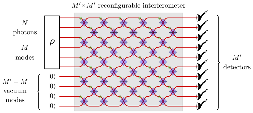
Figure 1: Tomography of a generic unknown state $\rho$ of $N$ photons in $M$ modes. Our protocol uses configurations of an $M^{\prime}$-mode linear optical interferometer followed by photon counting. When $M^{\prime}>M$, vacuum modes are appended to the state $\rho$.

Feasibility of tomography– Consider a generic quantum state of $N$ indistinguishable photons in $M$ modes. Our goal is to completely characterize the state by measuring multiple copies of it using linear optics and photon counting, as illustrated in Fig. 1. In this approach, a measurement basis corresponds to a particular configuration of linear optics. We also allow for measurements over $M^{\prime}\geq M$ modes, achieved by appending $M^{\prime}-M$ vacuum modes to the state of interest. Our first main result is that full tomography can always be achieved using a finite number of measurement configurations:

Theorem 1.

An $N$-photon, $M$-mode state can be reconstructed using photon counting and $M$-mode linear optical interferometer with a finite number $R$ of configurations, where

$$R<\binom{N+M^{2}-1}{N}^{2}.$$ (1)

The theorem is proved by building an explicit reconstruction algorithm. Let $|{\nu}\rangle$ be the multi-mode Fock basis $|{\nu}\rangle\equiv|{k_{1},\dots,k_{M}}\rangle$, where $k_{j}$ is the number of particles in mode $j$ and $\sum_{j}k_{j}=N$, while we use a prime to denote a Fock basis $|{\nu^{\prime}}\rangle\equiv|{k_{1},\dots,k_{M^{\prime}}}\rangle$, where the number of output modes $M^{\prime}$ may be higher than the number of inputs $M$. Moreover, let $U(g)$ be a set of available unitary operations that can be made in the system. In linear optics the most general SU(M^′) transformation can be obtained with a collection of beam splitters and phase shifters Clements et al. (2016), as shown in Fig. 1. Such transformation can be expressed in the second quantized notation as $U(g)=e^{i\sum_{kl}H_{kl}a_{k}^{\dagger}a_{l}}$, where $g=e^{iH}$ is a $M^{\prime}\times M^{\prime}$ unitary matrix.

State tomography requires reconstruction of the state $\rho$ from measurement outcomes, each specified by a series of photon counts $\nu^{\prime}$. These outcome probabilities are readily calculated as $p_{\nu^{\prime},g}=\langle{\nu^{\prime}}|U(g)^{\dagger}\rho U(g)|{\nu^{\prime}}\rangle$ for a specified interferometer configuration $g$. Expanding the above equation gives

$$p_{\nu^{\prime},g}=\sum_{\alpha,\beta}\langle{\nu^{\prime}}|U(g)^{\dagger}|{\alpha}\rangle\langle{\alpha}|\rho|{\beta}\rangle\langle{\beta}|U(g)|{\nu^{\prime}}\rangle\equiv[\mathcal{L}(\rho)]_{\nu^{\prime},g}~{},$$ (2)

with the superoperator $\mathcal{L}_{\nu^{\prime}g,\alpha\beta}=\langle{\nu^{\prime}}|U(g)^{\dagger}|{\alpha}\rangle\langle{\beta}|U(g)|{\nu^{\prime}}\rangle$. The superoperator $\mathcal{L}$ is constructed using different configurations $g_{j}$, with $j=1,\dots,R$. The numbers $\alpha$ and $\beta$ index the elements of the Fock space, whose dimension is $D_{N,M}=\binom{N+M-1}{N}$, while $\nu^{\prime}=1,\dots,D_{N,M^{\prime}}$. As such, $\mathcal{L}$ is normally a rectangular operator. Tomography is possible if there is a large enough $R$ such that the linear system (2) admits a unique solution for any $p$. A unique solution is obtained Klose et al. (2001) when the Gramian matrix $\mathcal{L}^{\dagger}\mathcal{L}$ has full rank. In this case, the best reconstruction algorithm Klose et al. (2001) is given by the pseudo-inverse $\rho_{\rm best}:=(\mathcal{L}^{\dagger}\mathcal{L})^{-1}\mathcal{L}^{\dagger}[p]$, which is always the best fit solution that minimizes the least-square error.

For any linear optics configuration $g$, the matrix elements $\langle{\beta}|U(g)|{\nu^{\prime}}\rangle$ can be calculated exactly, either using combinatorial expressions or matrix permanents Scheel (2004); Biedenharn et al. (1985); Aaronson and Arkhipov (2011): for $|{\alpha}\rangle=|{a_{1},a_{2},\dots}\rangle$ and $|{\beta}\rangle=|{b_{1},b_{2},\dots}\rangle$, one finds $\langle{\alpha}|U(g)|{\beta}\rangle={{\rm per}(g_{\{\alpha,\beta\}})}{/}{\sqrt{\alpha!\beta!}}$ where $\alpha!=a_{1}!a_{2}!\dots$, and similarly for $\beta!$, while $g_{\{\alpha,\beta\}}$ is the $N\times N$ matrix obtained by copying $a_{i}$ times the $i$-th columns of $g$ and, and $b_{j}$ times the $j$-th row of $g$. Although the computation of the matrix permanent is #P-hard, it is still possible for the values of $N$ and $M$ available in near-term devices Neville et al. (2017). Moreover, there are cases for which specific values of the permanent can be computed analytically Tichy et al. (2014); Dittel et al. (2017); Viggianiello et al. (2018). In the worst case, without making any simplifications about the permanents, in the Supplementary Material we show that the number of operations to reconstruct the state from Eq. (2) is $\mathcal{O}({\rm poly}(D_{N,M},2^{N}))$. Therefore, as in qubit systems, the difficulty is mostly due to exponentially growing Hilbert space, rather than to the complexity of the permanent.

Given the above framework, we now sketch our proof of Theorem 1, which is elaborated in the Supplementary Material. In particular, we show that with interferometer configurations $\{g_{j}\}_{j=1,\dots,R}$ corresponding to a unitary $2N$-design, exact reconstruction is possible from experimental measurements of $p_{\nu^{\prime},g_{j}}$ for all $j=1,\dots,R$. Our theorem then follows from known properties of unitary designs Roy and Scott (2009): they exist for all $N$ and $M$, and their size is bounded by $R<D_{N,M^{2}}^{2}$.

To connect our tomographic task to unitary designs, we first note that the matrix $\mathcal{L}$ is composed by $U(g)\otimes U(g)^{*}$ matrices. Although $U(g)$ is an irreducible representation of $g$, $U(g)\otimes U(g)^{*}$ is not, and indeed it can be written as a direct sum of Wigner-$D$ matrices $\mathcal{D}^{\lambda_{r}}_{m,m^{\prime}}$ where $\lambda_{r}$ refer to different irreducible representations and $m,m^{\prime}$ are Gelfand-Tsetlin patterns that index the different states (see Supplementary Material). Since the matrices $\mathcal{D}^{\lambda_{r}}_{m,m^{\prime}}(g)$ are orthogonal over $g$ and $\mathcal{L}\propto\mathcal{D}(g)$, one can use the matrix $\mathcal{D}(g)^{*}$ to construct an operator $X^{\nu^{\prime}}_{\alpha\beta}(g)$ such that $\langle{\alpha}|\rho|{\beta}\rangle=\sum_{\nu^{\prime}}\int dg\,X^{\nu^{\prime}}_{\alpha\beta}(g)p_{\nu^{\prime},g}$, where $p_{\nu^{\prime},g}$ are the outcome probabilities in Eq. (2).

Tomography is therefore achieved via a formal average over the continuous group. However, this is not practical as it would require an infinite number of measurement configurations. Instead we use the theory of weighted unitary designs Roy and Scott (2009), to replace the continuous average with a discrete average over a discrete set of unitaries $g_{j}$. A $q$-design is a discrete set of unitaries such that the weighted average of group functions $f(g)$ over those unitaries is equal to the average over the continuous group $\int dgf(g)$, provided that $f(g)$ is a polynomial of at most degree $q$ in $g$ and $g^{*}$. Since the matrices $\mathcal{D}(g)$ are a polynomial of at most degree $N$ in $g$ and $g^{*}$, one can choose any weighted $2N$-design protocol to analytically perform full-state tomography, as shown in the Supplementary Material. Calling $g_{j}$ those unitaries, $\langle{\alpha}|\rho|{\beta}\rangle=\sum_{\nu^{\prime},j}X^{\nu^{\prime}}_{\alpha\beta}(g_{j})p_{\nu^{\prime},g_{j}}$. This concludes the proof of Theorem 1. We note however that unitary $2N$-designs satisfy a more stringent requirement than the simpler inversion of Eq. (2), and consequently, this approach is generally not optimal in terms of the number of measurement configurations used. Theorem 1 can be trivially extended to mixtures $\rho=\sum_{N=1}^{N_{\rm max}}\pi_{N}\,\rho_{N}$ where $\rho_{N}$ is a $M$-mode $N$-photon state, as each $N$-photon state can be reconstructed independently via postselection (see Supplementary Material).

Minimum measurement configurations– We now consider the minimum number of linear optics configurations $R$ required to achieve tomography. Our second main result gives a lower bound on the number of configurations required:

Theorem 2.

An $N$-photon, $M$-mode state can be reconstructed with photon counting and an $M$-mode linear optical interferometer using at least

$$R_{N,M}=\binom{N+M}{N}-\binom{N+M-2}{M}$$ (3)

configurations. More generally, for an interferometer with $M^{\prime}>M\geq 2$ modes and ancillary vacuum states, the minimal number of reconfigurations is

$$R_{N,M,M^{\prime}}=\left[\frac{(N+M-2)!(M^{\prime}-2)!}{(N+M^{\prime}-2)!(M-2)!}R_{N,M}\right]~{},$$ (4)

where $[x]$ is the smallest integer greatest or equal to $x$.

Equation (3) shows that the number of measurement configurations is larger than estimated from a simple counting argument. In particular, the number of $M$-mode Fock states with $N$ total photons, $D_{N,M}=\binom{N+M-1}{N}$, gives the dimension of the symmetric Hilbert space. A generic state is thus specified by $D_{N,M}^{2}-1$ independent elements.

A single measurement configuration involves $D_{N,M}$ different outcomes, which provide $D_{N,M}-1$ independent parameters. Therefore, one may expect that $D_{N,M}+1$ configuration may be sufficient for full state reconstruction. Instead, our theorem shows a larger number is required, $R_{N,M}>D_{N,M}+1$. This increased requirement is due to linear optics providing only a subset of the possible unitary operations on the multi-particle state. Nonetheless, complete tomography with a smaller set of configurations is possible with ancillary output modes, as $R_{N,M,M^{\prime}}<D_{N,M}+1<R_{N,M}$ for any $M^{\prime}>M$.

For the two-mode case, $M=2$, an explicit measurement protocol which saturates our bound $R_{N,2}=2N+1$ is known Walser (1997). This protocol exploits the Schwinger boson formalism that maps our problem onto the tomography of a spin $S=N/2$, allowing the use of known algorithms for large spin systems Newton and Young (1968); Klose et al. (2001); Hofmann and Takeuchi (2004). However, this approach exploits properties of SU(2) representations that cannot be easily adapted to larger $M$ Filippov and Man’ko (2009); Tan et al. (2013). Our theorem generalizes the above construction to the general multi-mode case.

Two proofs of Theorem 2 are presented in the Supplementary Material, one based on representation theory and one based on irreducible tensors. Here we briefly describe the main steps of the second proof. Measuring diagonal elements in the Fock basis is equivalent to the measurement of all the expectation values of polynomials of number operators $T^{k}_{k}=a^{\dagger}_{k}a_{k}$. According to Wick’s theorem, all independent polynomials in the number operators can be written via the rank $r$ tensors $T^{k_{1},\dots,k_{r}}_{k_{1},\dots,k_{r}}=a^{\dagger}_{k_{1}}\cdots a^{\dagger}_{k_{r}}a_{k_{1}}\cdots a_{k_{r}}$. However, not all $\langle{T^{k_{1},\dots,k_{r}}_{k_{1},\dots,k_{r}}}\rangle$ are independent. For instance, if one measures $\langle{T^{k}_{k}}\rangle$ for $k=1,\dots,M-1$, then one gets $\langle{T^{M}_{M}}\rangle=N-\sum_{k=1}^{M-1}\langle{T_{k}^{k}}\rangle$ without further measurements. In the Supplementary Material we show that the number of independent rank-$r$ tensors is $D_{r,M-1}$. Their expectation value for $r=1,\dots,N$ completely and uniquely specify photodetection measurements. Similarly, the full state is completely and uniquely specified by the expectation value of the tensors $T^{k_{1},\dots,k_{r}}_{\ell_{1},\dots,\ell_{r}}=a^{\dagger}_{k_{1}}\cdots a^{\dagger}_{k_{r}}a_{\ell_{1}}\cdots a_{\ell_{r}}$. The number of such independent rank-$r$ tensors is $D_{r,M}^{2}-D_{r-1,M}^{2}$.

Tomography then consists in reconstructing the expectation value of off-diagonal tensors from the measurement of $\langle{T^{k_{1},\dots,k_{r}}_{k_{1},\dots,k_{r}}}\rangle$ after different configurations $U(g)$. Since the latter corresponds to $\langle{U(g)^{\dagger}T^{k_{1},\dots,k_{r}}_{k_{1},\dots,k_{r}}U(g)}\rangle=[g^{\dagger\otimes r}\langle{T}\rangle g^{\otimes r}]^{k_{1},\dots,k_{r}}_{k_{1},\dots,k_{r}}$, all off-diagonal tensors with different rank $r$ can be reconstructed independently for $r=1,\dots,N$. The most difficult tensor to reconstruct is then that with $r=N$. Via dimensional counting, this reconstruction requires $[D_{N,M}^{2}-D_{N-1,M}^{2}]/D_{N,M-1}\equiv R_{N,M}$ transformations. Equation (3) follows by assuming that the same configurations are sufficient for reconstructing even lower rank tensor. This latter assumption is the reason why Eq. (3) is a lower bound. Similarly, Eq. (4) appears for different number of modes as $R_{N,M,M^{\prime}}=[(D_{N,M}^{2}-D_{N-1,M}^{2})/D_{N,M^{\prime}-1}]\equiv[R_{N,M}D_{N,M-1}/D_{N,M^{\prime}-1}]$.

Theorem 2 can be extended to mixtures $\rho=\sum_{N=1}^{N_{\rm max}}\pi_{N}\,\rho_{N}$ where $\rho_{N}$ is a $M$-mode $N$-photon state. In this case, the minimal number of settings is $\max_{N\leq N_{\rm max}}R_{N,M,M^{\prime}}$ (see Supplementary Material). Theorem 2 also determines the number of ancillary modes needed to achieve tomography with a single measurement configuration:

Corollary.

An $N$-photon, $M$-mode state can be reconstructed with a single configuration of an $M^{\prime}$-mode linear optical interferometer if

$$D_{N,M^{\prime}-1}\geq D_{N,M}^{2}-D_{N-1,M}^{2}=R_{N,M}D_{N,M-1}~{}.$$ (5)

The scaling of Eq. (5) can be investigated for large $N$ and $M$ using the entropic expansion $\binom{n}{k}\approx 2^{nH_{2}(k/n)}$, where $H_{2}(x)={-}x\log_{2}x{-}(1{-}x)\log_{2}(1{-}x)$ is the binary entropy. If additionally $N\gg M$, we find that $R_{N,M}D_{N,M-1}\approx N^{2M-3}$, and $D_{N,M^{\prime}-1}\approx N^{M^{\prime}-2}$. Therefore the minimum number of measurement modes required is given by

$$M^{\prime}\stackrel{{\scriptstyle N\gg M}}{{\gtrsim}}2M-1~{}.$$ (6)

In this limit, tomography can be achieved using a single measurement configuration with photon counting over twice as many modes as the input state, and this result is independent of $N$.

In the opposite limit $N\ll M$, we approximate $\binom{N+M}{M}\approx M^{N}/N!$ to find

$$M^{\prime}\stackrel{{\scriptstyle N\ll M}}{{\gtrsim}}\frac{M^{2}}{\sqrt[N]{N!}}~{}.$$ (7)

This seemingly counterintuitive result shows that the required number of measured modes decreases as the number of photons increases. This is due to the large increase in number of measurement outcomes that results from an increase in the number of photons.

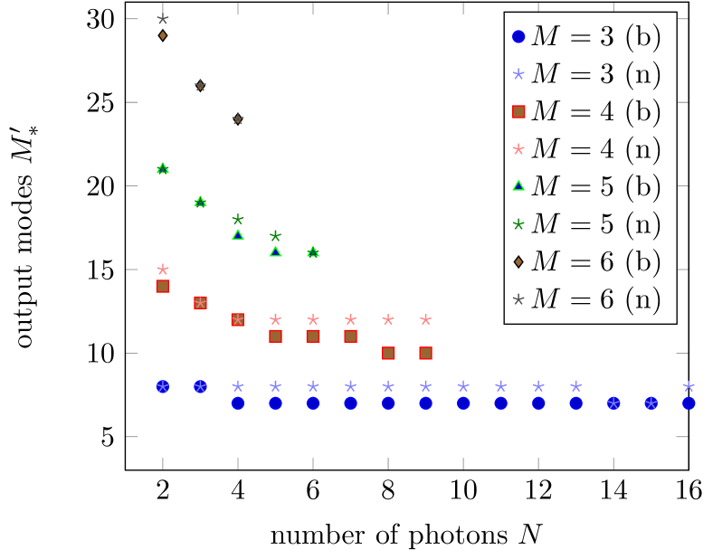
Figure 2: Number of measurement output modes required for full tomography with a single experimental setup. The lower-bound (b) is estimated from the minimal $M^{\prime}$ that satisfies Eq. (5). The observed numerical value (n) is obtained from the minimal $M^{\prime}$ such that Eq. (2) is invertible. For $M=2$ we always observe $M^{\prime}=4$, consistently with Eq. (5).

Practical implementation– We have done extensive numerical experiments showing that the bound (3) is achieved by Haar-random configurations $\{g_{\alpha}\}_{\alpha=1,\dots,R}$, which can be implemented using programmable interferometers Russell et al. (2017); Burgwal et al. (2017). In particular, we find that $\mathcal{L}$ has full-rank $D_{N,M}^{2}$ only when $R_{N,M}$, or more, configurations are used. For $M^{\prime}>M$, we find that the lower bound (4) is achievable with $R_{N,M,M^{\prime}}$, or slightly more, configurations. The slightly larger number of configurations or modes required for full-tomography when $M^{\prime}\neq M$ may be due to the simple reconstruction algorithm, which does not explicitly take into account independent components and normalization.

The minimum number of measurement modes $M^{\prime}$ required for a single interferometer is shown in Fig. 2, which shows agreement of numerical results calculated using a single sample from the Haar distribution and the minimal number that satisfies Eq. (6). As predicted by Eq. (7), $M^{\prime}$ initially decreases as a function of $N$ and then becomes constant for $N\approx M$. When $N\approx M$, we find $H_{2}\approx 1$ and hence $M^{\prime}\gtrsim\alpha M$, thus confirming the scaling relation (6), and its independence on $N$, although with a larger $\alpha>2$. Based on these numerical experiments, we conjecture that with a single Haar-random configuration one can perform full-reconstruction with a number of measurement modes that increases linearly with $M$.

In a realistic experiment, the number of detected photons will sometimes fluctuate, either because of imperfect photon sources (where $N$-photon states $\rho_{N}$ are generated with probability $\pi_{N}$), photon losses García-Patrón et al. (2017) or imperfect detector efficiency Lee et al. (2004); Achilles et al. (2004). When there are either imperfect sources or losses, the subset of detection events containing exactly the right number of photons is sufficient to reconstruct the state, provided these events occur at an acceptable rate. On the other hand, if losses are low and well characterized, one can use all the measured data to reconstruct the entire state $\rho=\sum_{N=1}^{N_{\rm max}}\pi_{N}\,\rho_{N}$ as we show in the Supplementary Material.

Single-photon detectors (SPDs) that merely distinguish between vacuum and non-vacuum states are often employed in realistic experiments, instead of true photon-counting detectors. To achieve sensitivity to photon number, a nondeterministic number resolving detector (NRD) can be built by multiplexing SPDs using linear optics and ancillary vacuum states Achilles et al. (2003); Řeháček et al. (2003); Fitch et al. (2003). We note that this concept is consistent with the scheme shown in Fig. 1, and therefore for sufficiently large $M^{\prime}$, complete state reconstruction can be achieved with SPDs. Since an NRD sensitive to $N$ photons requires $N$ SPDs, Eq. (6) implies that $\mathcal{O}(NM)$ SPDs are required. For $N\ll M$ fewer SPDs are required, due to the vanishing probability that multiple photons emerge in the same mode of a random interferometer with $M’>\mathcal{O}(N^{2})$ Aaronson and Arkhipov (2011). More precisely, from Eq. (7) we get $M^{\prime}>\mathcal{O}(M^{2}N/\sqrt[N]{N!})\approx\mathcal{O}(M^{2})$.

Conclusion– We have studied the feasibility and number of measurement configurations required to perform quantum tomography of a multi-mode multi-photon Fock state using linear optics and photon counting. We have shown that any such state can be tomographically reconstructed with a finite number of linear optics configurations (Theorem 1). To do so, we show that configurations corresponding to any unitary $2N$-design Roy and Scott (2009) defines an analytical, thought non optimal, reconstruction protocol. Moreover, Theorem 2 quantifies the minimal number of configurations, even when the number of detectors $M^{\prime}$ is larger than $M$. For sufficiently many detectors, as specified by Eq. (5), this leads to tomography with a single measurement configuration. Our results can be used to test the optimality of tomography protocols with a finite number of particles. For instance, the two-photon protocol presented in Walser (1997) saturates our bound, and is therefore optimal. Finally, we presented a simple reconstruction algorithm based on Haar sampled unitary configurations, and we have observed that it is optimal for $M^{\prime}=M$ and nearly optimality for $M^{\prime}>M$.

Appendix A SUPPLEMENTARY MATERIAL

Appendix B Bosonic representation of U(M)

Let us consider a set of bosonic creation and annihilation operators specified by $a^{\dagger}_{i\alpha}$ and $a_{j\beta}$. Using second quantization notation, we can define the operators

$$E_{ij}=\sum_{\alpha}a^{\dagger}_{i\alpha}a_{j\alpha}~{},$$ (8)

where $i,j=1,\dots,M$, and $\sum_{i}E_{ii}=N$. These operators satisfy the U(M) commutation relations

$$[E_{ij},E_{kl}]=\delta_{jk}E_{il}-\delta_{il}E_{kj}~{}.$$ (9)

Since bosonic operators are symmetric upon exchange of particles, the extra index $\alpha$ will be used to simulate other symmetries. For instance, a two-mode anti-symmetric wave function can be obtained with $(a_{1H}^{\dagger}a_{2V}^{\dagger}-a_{1V}^{\dagger}a_{2H}^{\dagger})|{0}\rangle$, where $|{0}\rangle$ is the bosonic vacuum and $\alpha=H,V$ is an external index, such as the horizontal (H) and vertical (V) photon polarization. The operators $H_{i}:=E_{ii}$ are called Cartan operators and form the maximal subset of commuting operators in the algebra. Operators $E_{ij}$ are called raising operators for $i<j$ and lowering operators for $i>j$. If an eigenstate $|{\psi}\rangle$ is an eigenstate of all Cartan operators $H_{i}|{\psi}\rangle=\lambda_{i}|{\psi}\rangle$ we say that the set $(\lambda_{1},\dots,\lambda_{M})$ is a weight of the state $|{\psi}\rangle$. Clearly $\sum_{i}\lambda_{i}=N$, where $N$ is the number of particles, as $\sum_{i}H_{i}=N$. Therefore, only $M-1$ Cartan operators $\tilde{H}_{i}=H_{i}-H_{i+1}$ are independent. A weight $(\lambda_{1},\dots,\lambda_{M})$ is said to be higher than $(\lambda^{\prime}_{1},\dots,\lambda^{\prime}_{M})$ if $\lambda_{1}>\lambda^{\prime}_{1}$, or if $\lambda_{1}=\lambda_{1}^{\prime}$ and $\lambda_{2}>\lambda^{\prime}_{2}$ etc. Irreducible representations (irreps) of the unitary group are uniquely characterized by their highest weight. All the other states in a certain irrep can be obtained from the highest weight state via multiple applications of the lowering operator Alex et al. (2011). A highest weight is a set of integers $\lambda_{1},\dots,\lambda_{M}$ that satisfy $\lambda_{i}\geq\lambda_{i+1}$. These numbers can be represented by a Young diagram $Y(\lambda)$, which is an array of left adjusted boxes, with $\lambda_{1}$ boxes on the first row, $\lambda_{2}$ boxes in the second row, etc. An alternative labeling of irreps is via Dynkin labels $(b_{1}b_{2}\dots)$ where $b_{j}$ is is the number of columns in the Young diagram with $j$ boxes.

The Gelfand-Tsetlin (GZ) basis Moshinsky (1966) is a convenient basis specified by a set of integers $m_{ij}$

$$\begin{pmatrix}m_{1,M}&&m_{2,M}&&m_{3,M}&&\dots&&m_{M,M}\\ &m_{1,M-1}&&m_{2,M-1}&&\dots&&m_{M-1,M-1}\\ &&&&\vdots&&&\\ &&&m_{1,2}&&m_{2,2}&&\\ &&&&m_{1,1}&&&\end{pmatrix}.$$

In this basis the $s$-th row $m_{rs}$ gives the irreducible representation of the subgroup U(s) in the chain decomposition U(M)$\supset$U(M-1)$\supset\dots\supset$U(1). The entries in lower rows satisfy the “betweenness condition” $m_{k,i}\geq m_{k,i-1}\geq m_{k+1,i}$ Alex et al. (2011). The first row then specifies the irreps with $\lambda_{i}=m_{i,M}$ while the other rows (that we collectively call $m$) specify the state in that particular irreps. These states will be labeled then as $|{\lambda,m}\rangle$. All Cartan operators $H_{i}$ are diagonal in the GZ basis, with eigenvalues (weights)

$$w_{i}=\sum_{k=1}^{i}m_{k,i}-\sum_{k=1}^{i-1}m_{k,i-1}~{}.$$ (10)

Because of the definition Eq. (8), the boson number operators are diagonal in the GZ basis, namely the GZ basis is like a Fock basis but with a convenient labelling. Highest weight states are such that $m_{ki}=m_{kM}\equiv\lambda_{k}$, namely where all the elements in the same diagonal are equal. These states, that we call $|{\lambda}\rangle$, have weights $w_{i}=\lambda_{i}$ and can be written in the second quantized form as Moshinsky (1966) $|{\lambda}\rangle\propto B(\lambda)|{0}\rangle$, where $|{0}\rangle$ is the bosonic vacuum, and $B(\lambda)$ is a polynomial in the creation operators Vilenkin and Klimyk (2013a)

$$B(\lambda)=\left(\Delta^{1}_{1}\right)^{\lambda_{1}-\lambda_{2}}\left(\Delta^{12}_{12}\right)^{\lambda_{2}-\lambda_{3}}\cdots\left(\Delta^{12\cdots M}_{12\cdots M}\right)^{\lambda_{M}}~{},$$ (11)

where $\Delta$ is the Slater determinant

$$\Delta^{i_{1},i_{2},\dots}_{j_{1},j_{2},\dots}=\det\begin{pmatrix}a^{\dagger}_{i_{1},j_{1}}&a^{\dagger}_{i_{1},j_{2}}&\dots\\ a^{\dagger}_{i_{2},j_{1}}&a^{\dagger}_{i_{2},j_{2}}&\dots\\ \vdots&\vdots&\ddots\end{pmatrix}~{}.$$ (12)

The fully symmetric representation with $N$ particles is then specified by the highest weight state with $\lambda=(N,0,\dots,0)$. Other states in the same irrep can be constructed from the repeated action of lowering operators. For instance, $E_{k+1,k}|{\{m_{i,j}\}}\rangle=\sum_{l}\alpha_{lk}(\{m\})|{\{m_{ij}-\delta_{il}\delta_{jk}\}}\rangle$, where the coefficients $\alpha$ are explicitly written in Vilenkin and Klimyk (2013b) (Chapter 18.1.2).

Generally we call a vector $|{\lambda,m}\rangle$ where $\lambda$ specifies the first row in the GZ pattern (and thus defines the irrep), while $m$ collects the other rows $m_{k,i}$ for $i<M$. An important vector for our discussion is $|{\lambda,0}\rangle$; using (10), we see that this vector is defined by the weight $w_{i}=0$ for $i<M$ and $w_{M}=\sum_{i}\lambda_{i}=N$. Therefore, for the bosonic representation $\lambda=[N]:=(N,0,\dots,0)$ this vector corresponds to the “boson condensate” state where all the particles are in the $M$-th mode. Other vectors in $[N]$ are parametrized by the GZ pattern

$$\begin{pmatrix}m_{1,M-1}&&0&&\dots&&0\\ &\ddots&&\vdots&&&\\ &&m_{1,2}&&0&&\\ &&&m_{1,1}&&&\end{pmatrix}.$$

where $m_{1,j}$ is related to the occupation number (10) via $w_{i}=m_{1,i}-m_{1,i-1}$, so here $w_{i}$ is the number of particles in mode $i$.

For a given irrep $\lambda$ the Wigner matrices are defined as

$$\mathcal{D}_{m,m^{\prime}}^{\lambda}(g)=\langle{\lambda,m}|U(g)|{\lambda,m^{\prime}}\rangle~{}.$$ (13)

These matrices are orthogonal with respect to the scalar product

$$\int dg\,\mathcal{D}_{m,m^{\prime}}^{\lambda}(g)\mathcal{D}_{\tilde{m},\tilde{m}^{\prime}}^{\tilde{\lambda}}(g)^{*}=\frac{\delta_{\lambda\tilde{\lambda}}}{d_{\lambda}}\delta_{m\tilde{m}}\delta_{m^{\prime}\tilde{m}^{\prime}}~{},$$ (14)

where $dg$ is the Haar measure and $d_{\lambda}$ is the dimension of the representation, given by Alex et al. (2011)

$$d_{\lambda}=\prod_{1\leq k<k^{\prime}\leq M}\left(1+\frac{\lambda_{k}-\lambda_{k^{\prime}}}{k^{\prime}-k}\right)~{}.$$ (15)

Given a representation $\lambda=(\lambda_{1},\dots,\lambda_{M})$ the conjugate representation can be defined as $\lambda^{*}=(-\lambda_{M},\dots,-\lambda_{1})$. Indeed, a representation of $g=e^{ih}$ is $U(g)=e^{i\sum_{jk}h_{jk}E_{jk}}$ and its conjugate is $U(g)^{*}=e^{-i\sum_{jk}h^{*}_{jk}E_{jk}}$, since the operators (8) are real (in the Fock basis). Therefore, the Cartan operators $H_{i}$ are mapped to $-H_{i}$ and so are the weights. However, with these definitions highest weights in the conjugate representation corresponds to lowest weights in the original one. The order reversal $\lambda^{*}=(-\lambda_{M},\dots,-\lambda_{1})$ assures that highest weights are mapped to highest weights. By definition the polynomial $B(\lambda^{*})$ associated with the conjugate representation can be obtained from (11) exchanging creation with annihilation operators. For each GZ pattern $m$ we can also get the corresponding dual pattern $m^{*}$ by reflecting each row $m_{k,i}^{*}=(-m_{i,i},\dots,-m_{1,i})$. Although the GZ pattern now contains negative numbers, this is not a problem because two patterns designate the same irrep if $m_{k,M}=m^{\prime}_{k,M}+c$ – this can be used to bring the GZ basis into the “normalized” form Alex et al. (2011) where $m_{M,M}=0$. However, the polynomials (11) are defined only when $m_{k,M}\geq 0$.

We consider the tensor product of the symmetric irrep $[N]:=(N,0,\dots,0)$ and its conjugate $[N]^{*}:=(0,\dots,0,-N)$, which in the normalized form is $(N,\dots,N,0)$. As in the addition of angular momenta, this product can be written as a direct sum of irreps. In general, see Vilenkin and Klimyk (2013b) Chapter 18.2.6, the product of an irrep $\{m_{k,M}\}$ with the fully symmetric one $(N,0,\dots,0)$ is a direct sum over the irreps $\{m_{k,M}+p_{k}\}$ where the non-negative $p_{k}$ satisfy $\sum_{k}p_{k}=N$ and

$$m_{1,M}+p_{1} \geq m_{1,M}\geq m_{2,M}+p_{2}\geq\dots\geq m_{M-2,M}\geq$$

$$\geq m_{M-1,M}+p_{M-1}\geq m_{M-1,M}\geq m_{M,M}+p_{M}\geq m_{M,M}~{}.$$

For the product of the symmetric irrep and its conjugate, the above equations force $p_{2}=\dots=p_{M-1}=0$. All the solutions can then be parametrized by an integer $0\leq\ell\leq N$ such that $p_{1}=\ell$ and $p_{M}=N-\ell$. The resulting irreps are then $(N+\ell,N,\dots,N,N-\ell)$ in the normalized form. These can be written in the more compact form $\lambda_{\ell}:=(\ell,0,\dots,0,-\ell)$. Important states for our analysis are the ones with zero weight. These are the states such that $\sum_{k=1}^{i}m_{k,i}=0$, namely the states such that, if you reflect the GZ pattern $m$ along the central vertical axis, you obtain $-m$. For $M=2$ and any $\ell$, the only state is the one with $m_{1,1}=0$. For $M=3$ all the $\ell+1$ states with $m_{1,1}=0$ and $m_{1,2}=-m_{2,2}$ with $0\leq m_{1,2}\leq\ell$ have zero weight. In general the number of zero weight states for fixed $\ell$ is

$$d^{0}_{\ell,M}=\begin{pmatrix}\ell+M-2\\ \ell\end{pmatrix}~{}.$$ (16)

Appendix C Proof of the main theorems

In Ref. Christandl and Renner (2012) (arXiv version) it has been shown that any bosonic density matrix (in fact any operator) with $N$ bosons and $M$ modes can be written in the integral form (P-representation)

$$\rho=\int_{\mathcal{U}_{M}}dx\,P_{\rho}(x)\,|{(x)_{N}}\rangle\langle{(x)_{N}}|$$ (17)

where the integration is over the continuous group $\mathcal{U}_{M}={\rm U}(M)/{\rm U}(M{-}1)\times{\rm U}(1)$,

$$|{(x)_{N}}\rangle=|{x}\rangle^{\otimes N}=\frac{\left(\sum_{j=1}^{M}x_{j}a_{j}^{\dagger}\right)^{N}}{\sqrt{N!}}|{0}\rangle~{},$$ (18)

is a bosonic condensate, and

$$P_{\rho}(x)=\sum_{\ell=0}^{N}\sum_{m}p_{\rho}(\ell,m)y_{\ell,m}(x)~{},$$ (19)

where $p_{\rho}(\ell,m)$ are coefficients, $m$ is a GZ pattern corresponding to the irrep $\lambda_{\ell}$, and $y_{\ell,m}(g)=\mathcal{D}^{\lambda_{\ell}}_{m,0}(g)$ is written in terms of the Wigner matrices (13). A generic $g\in{\rm U}(M)$ can be decomposed as $g=xh$ with $x\in\mathcal{U}_{M}$ and $h\in{\rm U}(M-1)\times{\rm U}(1)$. The bosonic condensate (18) can be written in terms of the state $|{\lambda,0}\rangle$ for $\lambda=[N]$. Indeed, as shown in the previous section, this state is the one where all the particles are in the $M$-th mode. Since this state is invariant under U($M-1$) one finds that then $|{(x)_{N}}\rangle=U(g)|{[N],0}\rangle\equiv U(x)|{[N],0}\rangle$. Because of this, from the orthogonality of Wigner matrices (14), one finds that

$$\int_{\mathcal{U}_{M}}\!\!\!dx\,y_{\ell,m}(x)y_{\ell^{\prime},m^{\prime}}(x)^{*} =\int_{{\rm U}(M)}\!\!\!\!dg\,\mathcal{D}_{m,0}^{\lambda_{\ell}}(g)\mathcal{D}_{m^{\prime},0}^{\lambda_{\ell^{\prime}}}(g)^{*}=$$ (20)

$$=\frac{1}{d_{\ell}}\delta_{\ell,\ell^{\prime}}\delta_{m,m^{\prime}}~{},$$ (21)

where $d_{\ell}=d_{\lambda_{\ell}}$.

Operators diagonal in the Fock basis are also diagonal in the GZ basis. One can therefore use the latter for calculations. Off-diagonal elements of the density matrix are then

$$\rho_{m,m^{\prime}}=\langle{[N],m}|\rho|{[N],m^{\prime}}\rangle~{}.$$ (22)

Using the P-representation (17), one has $\langle{[N],m}|(x)_{N}\rangle=\mathcal{D}^{[N]}_{m,0}(x)$, and similarly $\langle(x)_{N}|{[N],m}\rangle=(\langle{[N],m}|(x)_{N}\rangle)^{*}=\mathcal{D}^{[N]}_{m,0}(x)^{*}=\mathcal{D}^{[N]^{*}}_{m^{*},0}(x)$, so

$$\rho_{m,m^{\prime}} =\int dx\,P_{\rho}(x)\,\mathcal{D}^{[N]}_{m,0}(x)\mathcal{D}^{[N]^{*}}_{m^{\prime}{}^{*},0}(x)$$ (23)

$$=\int dx\,P_{\rho}(x)\,\left[\mathcal{D}^{[N]^{*}}_{m^{*},0}(x)\mathcal{D}^{[N]}_{m^{\prime},0}(x)\right]^{*}~{}.$$ (24)

An explicit form for the polynomial $\mathcal{D}^{[N]}_{m,0}(x)$ for $x\in\mathcal{U}_{M}$ is written in Vilenkin and Klimyk (2013a) (Chapter 5.2.5)

$$\mathcal{D}^{[N]}_{m,0}(x)=\frac{1}{\sqrt{d_{[N]}}}\prod_{j=1}^{M}\frac{x_{j}^{w_{j}}}{\sqrt{w_{j}!}}$$ (25)

where $w_{j}=m_{1,j}-m_{1,j-1}$. As we have shown in the previous section the tensor product of $[N]$ and $[N]^{*}$ is a sum of irreps $\lambda_{\ell}$. From the expansion of Wigner functions (see Vilenkin and Klimyk (2013b) Chapter 18.2.1)

$$\mathcal{Y}_{m^{\prime},m^{*}}(x) =\mathcal{D}^{[N]^{*}}_{m^{*},0}(x)\mathcal{D}^{[N]}_{m^{\prime},0}(x)$$ (26)

$$=\sum_{\ell=0}^{N}\sum_{\tilde{m},m_{0}}\Gamma^{N}_{\ell}(m^{\prime},m^{*}|\tilde{m},m_{0})\mathcal{D}^{\lambda_{\ell}}_{\tilde{m},m_{0}}(x)$$ (27)

where

$$\Gamma^{N}_{\ell}(m^{\prime},m^{*}|\tilde{m},m_{0})=\sum_{r} \langle{[N]^{*},m^{*};[N],m^{\prime}}|\lambda_{\ell},r,\tilde{m}\rangle\times$$ (28)

$$\times\langle\lambda_{\ell},r,m_{0}|{[N]^{*},0;[N],0}\rangle$$ (29)

and $\langle{\lambda,m;\lambda^{\prime},m^{\prime}}|\lambda^{\prime\prime},r,m^{\prime\prime}\rangle$ is the Clebsch-Gordan coefficient with multiplicity $r$ Vilenkin and Klimyk (2013b); Alex et al. (2011). The Clebsch-Gordan coefficients are real, and different from zero only if the weights (10) coincide Alex et al. (2011), namely if $w_{i}(m^{\prime})+w_{i}(m)=w_{i}(m^{\prime\prime})$ for any $i$. When $m^{\prime}=m^{*}$ the only possibility is when $m$ is a zero weight state. Therefore, from the orthogonality (21) we find

$$\rho_{m,m^{\prime}} =\int_{{\rm U}(M)}dg\,P_{\rho}(g)\,\mathcal{Y}^{*}_{m^{\prime},m^{*}}(g)=$$ (30)

$$=\sum_{\ell=0}^{N}\sum_{\tilde{m}}\frac{p_{\rho}(\ell,\tilde{m})}{d_{\ell}}\Gamma^{N}_{\ell}(m^{\prime},m^{*}|\tilde{m},0)~{},$$ (31)

$$\rho_{m,m} =\sum_{\ell=0}^{N}\sum_{\tilde{m}\in Z_{\ell}}\frac{p_{\rho}(\ell,\tilde{m})}{d_{\ell}}\Gamma^{N}_{\ell}(m,m^{*}|\tilde{m},0)~{},$$ (32)

where we used (27) and the orthogonality (14). In (31) where the range of $\tilde{m}$ is bounded for any $\ell$ by the “betweenness” condition, and $Z_{\ell}$ is the set of zero weight states in $\ell$. From the dimensionality (16), and since $\sum_{\ell=0}^{N}d^{0}_{\ell,M}=D_{N,M}$ we see that the diagonal elements of the density matrix are in one-to-one correspondence with the numbers $p_{\rho}(\ell,m)$ for $m\in Z_{\ell}$.

We now calculate the diagonal elements after the application of a rotation $g^{\prime}\in{\rm U}(M)$,

$$p_{n}(g^{\prime}) =\langle{[N],n}|U(g)\rho U(g)^{\dagger}|{[N],n}\rangle=$$ (33)

$$=\int_{{\rm U}(M)}dg\,P_{\rho}(g)\,\mathcal{Y}^{*}_{n,n^{*}}(g^{\prime}{}^{\dagger}g)~{}.$$

Since

$$\mathcal{D}^{\lambda_{\ell}}_{\tilde{m},m_{0}}(g^{\prime}{}^{\dagger}g)^{*} =\sum_{\lambda,m}\langle{\lambda_{\ell},\tilde{m}}|U(g^{\prime})^{\dagger}|{\lambda,m}\rangle^{*}\langle{\lambda,m}|U(g)|{\lambda_{\ell},m_{0}}\rangle^{*}$$ (34)

$$=\sum_{m}\mathcal{D}^{\lambda_{\ell}}_{m,\tilde{m}}(g^{\prime})\mathcal{D}^{\lambda_{\ell}}_{m,m_{0}}(g)^{*}$$ (35)

where in the first equation we introduce a resolution of the identity. Inserting the above equation in (33) and using the orthogonality (14) we find

$$p_{n}(g) =\sum_{\ell=0}^{N}\sum_{m}\sum_{m_{0}\in Z_{\ell}}\Gamma^{N}_{\ell}(n,n^{*}|m_{0},0)\frac{p_{\rho}(\ell,m)}{d_{\ell}}\mathcal{D}^{\lambda_{\ell}}_{m,m_{0}}(g)~{}.$$ (36)

The Clebsch-Gordon coefficients satisfy the orthogonality relations Vilenkin and Klimyk (2013b)

$$\sum_{mm^{\prime}}\langle\mu^{\prime},r^{\prime},n^{\prime}|{\lambda,m;\lambda^{\prime},m^{\prime}}\rangle\langle{\lambda,m;\lambda^{\prime},m^{\prime}}|\mu,r,n\rangle =\delta_{\mu,\mu^{\prime}}\delta_{nn^{\prime}}\delta_{rr^{\prime}}~{},$$

$$\sum_{\mu rp}\langle{\lambda,m;\lambda^{\prime},m^{\prime}}|\mu,r,p\rangle\langle\mu,r,p|{\lambda,n;\lambda^{\prime},n^{\prime}}\rangle =\delta_{m,n}\delta_{m^{\prime}n^{\prime}}~{}.$$

From these we find the orthogonality relation

$$\sum_{m,m^{\prime}}\Gamma^{N}_{\ell}(m,m^{\prime} |\tilde{m},m_{0})\Gamma^{N}_{\ell^{\prime}}(m,m^{\prime}|\tilde{m}^{\prime},m_{0}^{\prime})=\delta_{\ell,\ell^{\prime}}\times$$

$$\times\delta_{\tilde{m},\tilde{m}^{\prime}}\Gamma^{N}_{\ell}(0,0|m_{0},m_{0}^{\prime})~{}.$$ (37)

and

$$\sum_{\ell,\tilde{m}}\Gamma^{N}_{\ell}(m,m^{\prime}|\tilde{m},\tilde{m})=\delta_{m,0}\delta_{m^{\prime},0}~{}.$$ (38)

Moreover, when $\tilde{m}\in Z_{\ell}$ the selection rule shows that for each $m$ in $[N]$ there is only a single $m^{\prime}$ in $[N]^{*}$ such that $w_{j}(m)+w_{j}(m^{\prime})=0$; this state is $m^{\prime}=m^{*}$. Therefore, we can remove one element from the sum (37) and write

$$\sum_{n}\Gamma^{N}_{\ell}(n,n^{*} |\tilde{m}_{0},m_{0})\Gamma^{N}_{\ell^{\prime}}(n,n^{*}|\tilde{m}_{0}^{\prime},m_{0}^{\prime})=\delta_{\ell,\ell^{\prime}}\times$$

$$\times\delta_{\tilde{m}_{0},\tilde{m}_{0}^{\prime}}\Gamma^{N}_{\ell}(0,0|m_{0},m_{0}^{\prime})~{},$$

for $\tilde{m}_{0}\in Z_{\ell},\tilde{m}_{0}^{\prime}\in Z_{\ell^{\prime}}$. From the above relations

$$\sum_{n}\Gamma^{N}_{\ell}(n,n^{*}|m_{0},0)p_{n}(g)=\sum_{m}\frac{P_{\rho}(\ell,m)}{d_{\ell}}\Gamma^{N}_{\ell}(0,0|0,0)\mathcal{D}^{\lambda_{\ell}}_{m,m_{0}}(g)~{}.$$

Since $\Gamma^{N}_{\ell}(0,0|0,0)\neq 0$ for any $0\leq\ell\leq N$ (Christandl and Renner (2012) Corollary 3), we define then

$$p^{\ell}_{m_{0},g}=\sum_{n}\frac{\Gamma^{N}_{\ell}(n,n^{*}|m_{0},0)^{*}}{\Gamma^{N}_{\ell}(0,0|0,0)}p_{n}(g)=\sum_{m}\frac{P_{\rho}(\ell,m)}{d_{\ell}}\mathcal{D}^{\lambda_{\ell}}_{m,m_{0}}(g)~{}.$$ (39)

The above result shows that if we can find a discrete set of unitaries $g_{\alpha}$ such that $\mathcal{D}^{\lambda_{\ell}}_{m,m_{0}}(g)$ is invertible, then we can obtain $P_{\rho}(\ell,m)$ and hence $\rho_{m,m^{\prime}}$. Indeed, if there is a discrete set of unitaries $\{g_{\alpha}\}$ and a matrix $X$ such that

$$\sum_{m_{0},\alpha}X^{\ell}_{m^{\prime},m_{0}g_{\alpha}}\mathcal{D}^{\lambda_{\ell}}_{m,m_{0}}(g_{\alpha})=\delta_{m,m^{\prime}}~{},$$ (40)

then from Eq. (31)

$$\rho_{m,m^{\prime}} =\sum_{\ell=0}^{N}\sum_{\tilde{m},m_{0},\alpha}\Gamma^{N}_{\ell}(m^{\prime},m^{*}|\tilde{m},0)X^{\ell}_{\tilde{m},m_{0}g_{\alpha}}p^{\ell}_{m_{0},g_{\alpha}}~{}.$$ (41)

C.1 Proof of Theorem 1: Unitary design

An analytic solution to Eq. (40) is obtained from the theory of unitary designs Roy and Scott (2009). A set of unitaries ${g_{\alpha}}_{\alpha=1,\dots,R}$ is called a weighted unitary $t$-design if

$$\sum_{\alpha}w(g_{\alpha})g_{\alpha}^{\otimes t}\otimes g_{\alpha}^{*\otimes t}=\int_{U(M)}dg\,g^{\otimes t}\otimes g^{*\otimes t}~{},$$ (42)

where $dg$ is the Haar measure, and $w$ is a weight. In other terms, a weighted unitary $t$-design is a collection of unitaries such that the weighted average of any polynomial function $f_{t}(g)$, with maximal degree $t$ in both $g_{ij}$ and $g_{kl}^{*}$, is equal to the average over the entire continuous group $\int dg\,f_{t}(g)$. From the expansion (27) and from (25), we see that $\mathcal{D}_{m,m_{0}}^{\lambda_{\ell}}$, and in particular $\mathcal{D}_{m,m_{0}}^{\lambda_{N}}$, are at most polynomial functions of degree $N$ in $g$ and $g^{*}$. Therefore, if ${g_{\alpha}}_{\alpha=1,\dots,R}$ is a weighted $2N$-design, then a solution of (40) is obtained by setting $X^{\ell}_{m,m0,g}=d_{\ell}w(g)\mathcal{D}_{m,m_{0}}^{\lambda_{\ell}*}$. Indeed, from the definition of unitary design Eq. (40) becomes

$$\sum_{m_{0},\alpha}X^{\ell}_{m^{\prime},m_{0}g_{\alpha}}\mathcal{D}^{\lambda_{\ell}}_{m,m_{0}}(g) =d_{\ell}\sum_{m_{0},\alpha}w(g_{\alpha})\mathcal{D}^{\lambda_{\ell}}_{m^{\prime},m_{0}}(g_{\alpha})^{*}\mathcal{D}^{\lambda_{\ell}}_{m,m_{0}}(g_{\alpha})$$

$$=d_{\ell}\int dg\,\mathcal{D}^{\lambda_{\ell}}_{m^{\prime},m_{0}}(g)^{*}\mathcal{D}^{\lambda_{\ell}}_{m,m_{0}}(g)=\delta_{m,m^{\prime}}~{},$$

where in the last equation we used the orthogonality of Wigner matrices. Therefore, for any weighted unitary $2N$-design, one can find an analytic solution to the tomographic reconstruction of the state

$$\rho_{m,m^{\prime}} =\sum_{\ell=0}^{N}\sum_{\tilde{m},m_{0},\alpha}\Gamma^{N}_{\ell}(m^{\prime},m^{*}|\tilde{m},0)d_{\ell}w(g_{\alpha})\mathcal{D}^{\lambda_{\ell}}_{\tilde{m},m_{0}}(g_{\alpha})^{*}p^{\ell}_{m_{0},g_{\alpha}}~{}.$$

Note that the requirement that the matrices $g_{\alpha}$ form a unitary $2N$-design is much stronger than (40). Indeed, with a unitary design, the average over any polynomial function is equal to the group integral, while for inverting (40) it is required that the discrete average is equal to the group integral only for specific set of functions (product of Wigner matrices). Upper and lower bounds on the size of a $2N$-design is given in Roy and Scott (2009), where they found that

$$B(M,N)\leq R\leq B(M,2N)~{},$$ (43)

where

$$B(M,N)=\sum_{\lambda:|\lambda_{+}|\leq N}d_{\lambda,M}^{2}~{}.$$ (44)

where $|\lambda_{+}|$ is the sum of the positive elements in $\lambda$ and $d_{\lambda,M}$, with explicit dependence on $M$, is written in (15). Moreover, Roy and Scott (2009)

$$B(M,N)\leq\binom{M^{2}+N-1}{N}^{2}\equiv D_{N,M^{2}}^{2}.$$ (45)

C.2 Proof of Theorem 2

Let $R$ be the number of unitaries ${g_{\alpha}}_{\alpha=1,\dots,R}$. The matrix $Y^{\ell}_{m,m0\alpha}=\mathcal{D}^{\lambda_{\ell}}_{m,m_{0}}(g_{\alpha})$ has dimension $d_{\ell}\times(Rd_{\ell,M}^{0})$. As in the main text, we focus on the higher dimensional irrep, namely $\ell=N$, and we want to count the number $R$ of matrices $g_{\alpha}$ required to make the matrix $Y^{N}$ invertible. Note that the Wigner $D$ functions $\mathcal{D}^{\lambda_{\ell}}_{m,m_{0}}(g_{\alpha})$ play the same role of the irreducible symmetric tensor of rank $r=\ell$ discussed in the main text. For $r=N$, thanks to Eq. (16), we find $d_{N,M}^{0}=D_{N,M-1}$. On the other hand, explicitly solving Eq. (15), we find $d_{N}=R_{N,M}D_{N,M-1}$. Therefore, in order to make $Y$ invertible for $\ell=N$, one finds $R\geq R_{N,M}$. This completes the proof of theorem  2, as the inverse in (40) exists. The lower bound can be achieved if the same unitaries $g_{\alpha}$ enable also the inversion $Y^{\ell}$ for $\ell<N$. The reconstruction algorithm is then Eq. (41).

Finally, we consider the case where the number of output modes $M^{\prime}$ is different from the number of inputs. Technically, all equations are still valid, because we can first expand the input space into $M^{\prime}>M$ modes, and select only inputs coming from $M$ mode subspace. One can still write then Eq. (40) and (41). As for Eq. (40), for the worst case scenario $\ell=N$, the number of possible $m_{0}$ is now $d^{0}_{N,M^{\prime}}=D_{N,M^{\prime}-1}$, while the number of $m$ is $d_{N}=R_{N,M}D_{N,M-1}$. From this we find an alternative proof our corollary Eq. (5).

C.3 Analytical solutions for M=2

SU(2) is formed by the matrices

$$U(g)=e^{i\phi S_{z}}e^{i\theta S_{y}}e^{i\eta S_{z}}~{},$$ (46)

where $S_{\alpha}$ are the spin matrices in an arbitrary representation. The states $|{\lambda_{l},m}\rangle$ are parametrized by a single integer $-\ell\leq m\leq\ell$. Moreover, there is only one zero-weight state $m_{0}=0$. To map these indices to standard spin notation we parametrize these numbers with semi-integers $S=\ell/2$ and $M=m/2$ (in this section $M$ is not the number of modes, which is always two), therefore

$$\mathcal{D}^{\lambda_{\ell}}_{m,m_{0}}(g)=y_{\ell,m}(g)=e^{i\phi M}d_{M,0}^{S}(\theta)~{},$$ (47)

where $d_{M,M^{\prime}}^{S}(\theta)=\langle{S,M}|e^{i\theta S_{y}}|{S,M^{\prime}}\rangle$ is the Wigner function, and the dependence of $\eta$ disappears. If we choose $X^{S}_{M}(\theta,\phi)=\gamma e^{-i\phi M}[d_{M,0}^{S}(\theta)]^{-1}$, where $\gamma$ is a normalization, and hence we need to select $\theta$ such that $d_{M,0}^{S}(\theta)\neq 0$ then the condition (40) can be written as

$$\gamma\sum_{\alpha}e^{i\phi_{\alpha}(M-M^{\prime})}\frac{d_{M,0}^{S}(\theta_{\alpha})}{d_{M^{\prime},0}^{S}(\theta_{\alpha})}=\delta_{M,M^{\prime}}~{},$$ (48)

where $-2S\leq M-M^{\prime}\leq 2S$, namely $-\ell\leq M-M^{\prime}\leq\ell$. In the worst case scenario, $-N\leq M-M^{\prime}\leq N$. Therefore, using standard properties of discrete Fourier Transform, a solution of the above equation, valid for any $M$ and $M^{\prime}$, is

$$\theta_{\alpha} =\theta~{}, \phi_{\alpha} =\frac{2\pi\alpha}{2N+1}~{}, \gamma=\frac{1}{2N+1}~{},$$ (49)

for $\alpha=0,\dots,2N$, where $\theta$ is such that $d_{M,0}^{S}(\theta)\neq 0$ for any $M$. This solution is therefore equivalent to the Newton and Young algorithm for SU(2) tomography Newton and Young (1968). As the number of setups is $R=2N+1$, this protocol saturates the bound (3).

Appendix D Alternative proof of the minimal number of configurations

We first present an alternative proof of Eq. (3). We note that photodetection is equivalent to the measurement of all the expectation values of polynomials of number operators $T^{k}_{k}=a^{\dagger}_{k}a_{k}$. Not all of these expectation values are independent. For instance, if one measures $\langle{T^{k}_{k}}\rangle$ for $k=1,\dots,M-1$, then one gets $\langle{T^{M}_{M}}\rangle=N-\sum_{k=1}^{M-1}\langle{T_{k}^{k}}\rangle$ without further measurements. Thanks to Wick’s theorem, all independent polynomials in the number operators can be written via the rank $r$ tensors $T^{\alpha_{1},\dots,\alpha_{r}}_{\alpha_{1},\dots,\alpha_{r}}=a^{\dagger}_{\alpha_{1}}\cdots a^{\dagger}_{\alpha_{r}}a_{\alpha_{1}}\cdots a_{\alpha_{r}}$, where we fix the convention that Greek indices $\alpha_{j}$ range from 1 to $M-1$ while Latin indices $k_{j}$ range from 1 to $M$. Tensors with some indices $M$ can be written in terms of other tensors with indices from 1 to $M-1$. For fixed rank $r$, the number of independent expectation values $\langle{T^{\alpha_{1},\dots,\alpha_{r}}_{\alpha_{1},\dots,\alpha_{r}}}\rangle$ is $D_{r,M-1}$. Moreover, such expectation values are zero for $r>N$. The expectation values $\langle{T^{\alpha_{1},\dots,\alpha_{r}}_{\alpha_{1},\dots,\alpha_{r}}}\rangle$ for $r=1,\dots,N$ uniquely specify the outcome of photodetection. Indeed, $\sum_{r=1}^{N}D_{r,M-1}=D_{N,M}-1$ so all the information about photodetection is contained in the expectation values of the independent tensors $T^{\alpha_{1},\dots,\alpha_{r}}_{\alpha_{1},\dots,\alpha_{r}}$.

Consider now a linear optical transformation, namely a collection of beam splitters and phase shifters, expressed by an irreducible representation $U(g)=e^{i\sum_{kl}H_{kl}a_{k}^{\dagger}a_{l}}$ of a SU(M), where $g=e^{iH}$ is a $M\times M$ unitary matrix. Applying first a linear optical network and then performing photodetection is equivalent to the measurement of the diagonal elements of $U(g)\rho U(g)^{\dagger}$ or, equivalently in the Heisenberg picture, of the independent tensors $U(g)^{\dagger}T^{\alpha_{1},\dots,\alpha_{r}}_{\alpha_{1},\dots,\alpha_{r}}U(g)$. With many choices of $g$ one then aims at measuring all the rank $r$ tensors

$$T^{k_{1},\dots,k_{r}}_{\ell_{1},\dots,\ell_{r}}=a^{\dagger}_{k_{1}}\cdots a^{\dagger}_{k_{r}}a_{\ell_{1}}\cdots a_{\ell_{r}}~{},$$ (50)

for $1\leq r\leq N$. Note that the above tensor has Latin indices, each ranging from $1$ to $M$. In fact $U(g)^{\dagger}T^{\alpha_{1},\dots,\alpha_{r}}_{\alpha_{1},\dots,\alpha_{r}}U(g)$ may have some indices equal to $M$. The above tensor is totally symmetric in its upper and lower indices, but not in mixtures of them. The numbers $\langle{T^{k_{1},\dots,k_{r}}_{\ell_{1},\dots,\ell_{r}}}\rangle$ provide $D_{r,M}^{2}$ expectation values, but not all of them are independent, since $\langle{T^{M,k_{2},\dots,k_{r}}_{M,\ell_{2},\dots,\ell_{r}}}\rangle$ can be written in terms of other expectation values. These dependent operators are $D_{r-1,M}^{2}$. Therefore, the number of independent rank $r$ expectation values is $D_{r,M}^{2}-D_{r-1,M}^{2}$. The independent expectation values are the numbers $\langle{T^{k_{1},\dots,k_{r}}_{\ell_{1},\dots,\ell_{r}}}\rangle$ where there is never both an upper and lower index $M$. These numbers completely and uniquely specify the state $\rho$, and indeed $\sum_{r=1}^{N}D_{r,M}^{2}-D_{r-1,M}^{2}=D_{N,M}^{2}-1$, which is the number of independent components in the density matrix $\rho$. Rank $r$ tensors transform as $U(g)^{\dagger}T^{k_{1},\dots,k_{r}}_{\ell_{1},\dots,\ell_{r}}U(g)=[g^{\dagger\otimes r}Tg^{\otimes r}]^{k_{1},\dots,k_{r}}_{\ell_{1},\dots,\ell_{r}}$, so each photodetection after the linear transformation $g$ allows us to measure the independent components $[g^{\dagger\otimes r}Tg^{\otimes r}]^{\alpha_{1},\dots,\alpha_{r}}_{\alpha_{1},\dots,\alpha_{r}}$. What is the minimal number of $g$ to reconstruct all off-diagonal elements $\langle{T^{k_{1},\dots,k_{r}}_{\ell_{1},\dots,\ell_{r}}}\rangle$? Fox fixed $r$ all the tensor components are independent (provided that index $M$ is not both on upper and lower indices), so the most difficult tensor elements to reconstruct are those for $r=N$. The number of independent components in this tensor is $D_{N,M}^{2}-D_{N-1,M}^{2}$, but each photodetection with a fixed choice of $g$ allows us to get $D_{N,M-1}$ independent values. Therefore, the minimal number of $g$ is $[D_{N,M}^{2}-D_{N-1,M}^{2}]/D_{N,M-1}\equiv R_{N,M}$. This concludes the proof of Eq. (3). Similarly, Eq. (4) appears for different number of modes as $R_{N,M,M^{\prime}}=[(D_{N,M}^{2}-D_{N-1,M}^{2})/D_{N,M^{\prime}-1}]\equiv[R_{N,M}D_{N,M-1}/D_{N,M^{\prime}-1}]$.

Note that this construction does not show that this lower bound is achievable, because the values of $g$ used to construct the rank $N$ expectation values may not enable the reconstruction of the other expectation values with $r<N$. Nonetheless, an explicit protocol which achieves our lower bound is known Walser (1997) for $M=2$.

D.1 Analytical reconstruction algorithm for $M=2$

It is instructive to rephrase the analytic protocol discussed in Section C.3 for $M=2$, based on the spin tomography protocols Newton and Young (1968), to see why the settings developed for the reconstruction of rank $N$ tensors are normally enough for the reconstruction of lower-rank tensors. According to Newton and Young (1968), SU(2) tomography can be achieved with $R_{N,2}=2N+1$ unitary matrices $g$, obtained by first applying different rotations $\phi_{j}$ along the $z$ axis, with $\phi_{j}=2\pi j/(2N+1)$ and $j=1,\dots,2N+1$, and then a fixed rotation with angle $\theta$ along the $y$ axis (see also Appendix C.3). In the linear optics setup, this corresponds to the application of different phase shifts $\phi_{j}$ on a single mode, followed by a beam splitter with transmissivity related to $\theta$. We set then $U(g)=e^{\theta(a_{1}^{\dagger}a_{2}-a_{2}^{\dagger}a_{1})}e^{i\phi a_{2}^{\dagger}a_{2}}$ and we note that for $M=2$ the Greek indices can only take the single value $\alpha_{j}=1$. Therefore, $p(\phi,\theta)=\langle{[g^{\dagger\otimes r}Tg^{\otimes r}]^{\alpha_{1},\dots,\alpha_{r}}_{\alpha_{1},\dots,\alpha_{r}}}\rangle=\sum_{\{k_{j}\},\{\ell_{j}\}}\langle{T^{k_{1},\dots,k_{r}}_{\ell_{1},\dots,\ell_{r}}}\rangle\prod_{j=1}^{r}(g_{k_{j},1}^{*}g_{\ell_{j},1})$, where the left-hand side contains the measured values and the right hand side contains the off-diagonal elements that we want to reconstruct. Calling $f_{k\ell}(\theta)$ the $\theta$ dependent part, we can write $p(\phi,\theta)=\sum_{\{k_{j}\},\{\ell_{j}\}}f_{k\ell}(\theta)\langle{T^{k_{1},\dots,k_{r}}_{\ell_{1},\dots,\ell_{r}}}\rangle e^{i\phi(n_{\{\ell{=}2\}}-n_{\{k{=}2\}})}$, where $n_{\{\ell{=}2\}}$ is the number of indices $\ell_{j}=2$ and similarly for $n_{\{k{=}2\}}$. Since independent tensors cannot have indices equal to 2 in both upper and lower indices, the number $I=n_{\{\ell{=}2\}}-n_{\{k{=}2\}}=-r,\dots,r$ completely specify the indices of the independent tensors. To reconstruct $\langle{T^{k_{1},\dots,k_{r}}_{\ell_{1},\dots,\ell_{r}}}\rangle$ one then simply has to choose different phases $\phi_{j}$ such that the matrix $e^{i\phi_{j}I}$ with $I=-r,\dots,r$ can be inverted for any $r$. Clearly one can consider the worst case $r=N$ and chose the Fourier transform where $\phi_{j}=2\pi j/(2N+1)$, so that $\langle{T(I)}\rangle\propto\sum_{j}e^{-i\phi_{j}I}p(\phi_{j},\theta)/f_{I}(\theta)$, where $I$ groups the indices $k$ and $\ell$. We remark that this choice is obtained by trying to invert the most complicated case $r=N$, but since $\sum_{j}e^{i\phi_{j}(I-J)}\propto\delta_{I,J}$ for any $-N\leq I,J\leq N$, with the same rotations one automatically obtains the lower rank tensors, where the only difference is that $I,J$ are constrained to smaller ranges. We conjecture that a similar construction applies also for higher values of $M$, and that the bound $R_{N,M}$ can always be achieved. This is indeed what we have observed in numerical simulations for different values of $M$ and $N$ and $R_{N,M}$ Haar-random choices of $g$.

Appendix E Imperfections

Here we study in more detail how to deal with possible errors in photon sources and detectors. Eventual photon losses in the interferometer can be included into the detector efficiency. Indeed, consider a model of an imperfect measurement as an extended linear optical interferometer wherein some ancillary modes are unmeasured García-Patrón et al. (2017). For uniform efficiency per mode $\eta$, the input-output relationship García-Patrón et al. (2017) is described by $\eta U$ where $U$ is a unitary $M^{\prime}\times M^{\prime}$ matrix (as in Fig. 1 of the main text). The resulting probability, given by Eq. 2 of the main text, is then $p_{\nu^{\prime},g,\eta}=\eta^{N}p_{\nu^{\prime},g}$ where $\eta^{N}$ is the probability of loosing no photons, and $p_{\nu^{\prime},g}$ is the conditional output probability, given that no photons have been lost. Because of this, photon losses can be modeled via auxiliary beam splitters that bring some photons to an unmeasured environment. An imperfect detector can also be modeled as a perfect detector with an extra beam splitter in front. Therefore, assuming that losses are uniform and independent on the configuration of the interferometer, we can include them into the detector efficiency.

We first consider the simplified case where either the photon sources or the detectors are imperfect, where a simple post-selection can be applied to reconstruct the correct state. The case where both imperfect sources and detectors are present is treated then in Sec. E.3.

E.1 Imperfect sources, perfect detectors

Suppose that the source emits $N$ photons with probability $\pi_{N}$. The resulting state is then

$$\rho=\sum_{N=0}^{N_{\rm max}}\pi_{N}\rho_{N}~{},$$ (51)

where each $\rho_{N}$ is a possibly mixed state with $N$ photons in $M$ modes. This probabilistic description is appropriate for common source imperfections, such as emission of a single emitter into an undesired spatial mode and inefficient heralding from a two-mode state generated by spontaneous parametric wave-mixing. Assuming perfect detectors, our protocol can be trivially extended to measure not only $\rho_{N}$ for the expected number of photon $N$, but also the entire state $\rho$ with the resulting probabilities $\pi_{N}$. Indeed, we can expand the photon probability after detection as

$$p_{n}(g) =\langle{n}|U(g)\rho U(g)^{\dagger}|{n}\rangle$$ (52)

$$=\sum_{N}\pi_{N}\,\langle{[N],n}|U(g)\rho_{N}U(g)^{\dagger}|{[N],n}\rangle$$ (53)

$$=\sum_{n}\pi_{N}p^{N}_{n}(g)~{},$$ (54)

where $|{n}\rangle=|{n_{1},\dots,n_{m}}\rangle$ is a generic multimode Fock state and $|{[N],n}\rangle$ is a Fock state such that $\sum_{j}n_{j}=N$. By post-selecting the measurement outcomes such that there are exactly $N$ photons one can reconstruct the conditional probability

$$p_{n}^{N}(g)=\langle{[N],n}|U(g)\rho_{N}U(g)^{\dagger}|{[N],n}\rangle~{}.$$ (55)

These probabilities can then be used to reconstruct the state following the procedure outlined in the main text. In other terms, post-selection allows us to treat the photon state in Eq. (51) as having exactly $N$ particles. The number of measurement settings is then $R_{N,M}$, or $R_{N,M,M^{\prime}}$ when the number of output modes is different. Nonetheless, one can go much further: by post-selecting over different photon numbers one can then reconstruct all the states $\rho_{N}$ for $N=1,\dots,N_{\rm max}$. From the same outcomes one can then estimate $\pi_{N}$, as the posterior probability of detecting $N$ photons.

We have observed in all numerical experiments that the same settings $g$ used to reconstruct $\rho_{N}$ can also be used to reconstruct the other states $\rho_{N^{\prime}}$ with $N^{\prime}\neq N$. Assuming that this numerical observation holds true in general, the required number of settings for complete reconstruction is then

$$\max_{N\in\{1,\dots,N_{\rm max}\}}R_{N,M,M^{\prime}}~{}.$$ (56)

The above number also provides the lower bound on the number of settings required for state tomography when the number of photons is uncertain. Remarkably, this number can be finite even when $N_{\rm max}$ is unbounded. This is due to the fact that, as we have discussed in the main text and shown in Fig. (2), $R_{N,M,M^{\prime}}$ can decrease as a function of $N$, for certain choices of $M^{\prime}$.

E.2 Perfect sources, imperfect detectors

Consider a single detector with efficiency $\eta$. The probability to detect $k$ photons when there are $n$ incident photons is given by

$$P_{\eta}(k|n)=\binom{n}{k}\;\eta^{k}(1-\eta)^{n-k}~{}.$$ (57)

A simple way to explain the above formula is that a photodetector with its detection efficiency $\eta$ can be interpreted as a perfect detector with a beam splitter in front. Here the beam splitter’s transitivity is determined by the detection efficiency. In case of multiple detectors $n=\{n_{1},\dots,n_{M}\}$, $k=\{k_{1},\dots,k_{M}\}$ and

$$P_{\eta}(k|n)=\prod_{j=1}^{M}P_{\eta_{j}}(k_{j}|n_{j})~{},$$ (58)

where $\eta_{j}$ is the efficiency of the detector on mode $j$.

The simplest way to deal with imperfect detectors is again post-selection: assuming that the input state has exactly $N$ photons, one can ignore all measurement outcomes where the total number of detected photons is different from $N$. This approach is viable as long as the data rate is sufficient.

Nonetheless, it has been shown in Lee et al. (2004); Achilles et al. (2004) that neglecting outcomes (namely post-selection) is not necessary, as long as the detection efficiency is well characterized. Indeed, suppose that the true photon distribution is $p^{N}_{n}(g)$, where $\sum_{j}n_{j}=N$, then the detected distribution is

$$p^{d}(k,g)=\sum_{n}P_{\eta}(k|n)p^{N}_{n}(g)~{}.$$ (59)

Different methods have been proposed Lee et al. (2004); Achilles et al. (2004) to reconstruct $p^{N}_{n}(g)$ given the detected probability $p^{d}(k,g)$, e.g. based on inverting the above matrix equation, or with maximum likelihood estimators or finally using Bayes’ theorem.

E.3 Imperfect sources, imperfect detectors

When there are both imperfect sources and imperfect detectors, then post-selection is not anymore a viable solution. Suppose indeed that the initial state is the one of Eq. (51), where the expected number of photons is $N$, while larger or smaller values are due to imperfect sources. It could be that the source generates a higher photon-number, but then one photon is lost so the number of detected photons is still $N$. Post-selection is clearly not able to remove this source of errors, so one has to rely on the inversion of Eq.(59), which is expected to be highly accurate when the detectors’ efficiency is sufficiently high.

More precisely, we can combine (54) with (59) to write

$$p^{d}(k,g) =\sum_{n}P_{\eta}(k|n)p_{n}(g)$$ (60)

$$=\sum_{n}P_{\eta}(k|n)\sum_{N}\pi_{N}p^{N}_{n}(g)~{}.$$

One can reconstruct the entire probability $p_{n}(g)$ by “inverting” the first equation, as described in Lee et al. (2004); Achilles et al. (2004), and then finding $\pi_{N}$ and $p^{N}_{n}(g)$ by conditioning. The resulting reconstruction protocol would then be equivalent to the one presented in Sec. E.1

Appendix F Remark about numerical experiments

The numerical experiments are performed by generating $R$ Haar random unitary matrices $g$, calculating the superoperator $\mathcal{L}_{\nu^{\prime}g,\alpha\beta}=\langle{\nu^{\prime}}|U(g)^{\dagger}|{\alpha}\rangle\langle{\beta}|U(g)|{\nu^{\prime}}\rangle$, and then finally studying the rank of the Gramian matrix $\mathcal{L}^{\dagger}\mathcal{L}$. Complete tomography is possible when such Gramian matrix has full-rank. We have observed that numerically generated Haar random matrices were always capable of producing a full rank Gramian when $R\geq R_{N,M}$ unitary matrices are employed. This numerically shows that our lower bound is achievable with Haar random configurations, at least for the sizes tested ($M\leq 6$ and $N\leq 10$).

Moreover, we have also numerically generated random linear optics configurations following the universal construction of Ref. Clements et al. (2016). We have observed that even when we consider random matrices obtained with random phase shifters and beam splitters (i.e. phase shifters and transmissivities sampled from independent uniform distributions), we obtain the same results. Such random matrices are not necessarily Haar random, but still they are “random enough” to provide the necessary information for complete state reconstruction. A more sophisticated construction can be obtained following the techniques of Ref. Russell et al. (2017). On the other hand, random phase shifts and fixed transmissivities are sufficient for $M=2$, as also shown by the Newton and Young algorithm Newton and Young (1968), but not for $M>2$. Therefore, we conjecture that linear optics configurations with uniformly random phase shifters and trasnmissivities are sufficient for complete tomography with minimal measurement settings.

Appendix G Numerical complexity of state reconstruction

We study the numerical complexity of a simple state reconstruction protocol, based just on the maximum likelihood estimator

$$\rho_{\rm MLE}:=(\mathcal{L}^{\dagger}\mathcal{L})^{-1}\mathcal{L}^{\dagger}[p]~{},$$ (61)

where $\mathcal{L}_{\nu^{\prime}g,\alpha\beta}=\langle{\nu^{\prime}}|U(g)^{\dagger}|{\alpha}\rangle\langle{\beta}|U(g)|{\nu^{\prime}}\rangle$, and $p_{\nu^{\prime},g}=\langle{\nu^{\prime}}|U(g)^{\dagger}\rho U(g)|{\nu^{\prime}}\rangle$ are the measured probabilities. Here we do not study any possible simplification in the evaluation of matrix permanents and consider the cost of evaluating the independent permanents $\langle{\beta}|U(g)|{\nu^{\prime}}\rangle$, without any other assumption. Indeed, as discussed in the main text, $\langle{\beta}|U(g)|{\nu^{\prime}}\rangle$ can be written as the permanent of a $N\times N$ matrix. Using Ryser’s formula Ryser (1963) the cost of evaluating such permanent is $\mathcal{O}(2^{N-1}N)$ arithmetic operations. Such cost is independent on the number of input and output modes $M$ and $M^{\prime}$. This estimate can be highly improved, for instance it is known that when there are many collisions (e.g. $M>N$) the permanent is easier Aaronson and Arkhipov (2011). However, here we do not consider any simplifying assumption and study just the numerical complexity with Ryser’s algorithm. In that case, one has to evaluate

$$\mathcal{O}(R_{N,M,M^{\prime}}D_{N,M}D_{N,M^{\prime}})\approx\mathcal{O}\left(R_{N,M}\frac{D_{N,M-1}}{D_{N,M^{\prime}-1}}D_{N,M}D_{N,M^{\prime}}\right)$$ (62)

of such permanents.

When $N\gg M,M^{\prime}$ then $R_{N,M}\approx D_{N,M}\approx N^{M-1}$ so the complexity of building $\langle{\beta}|U(g)|{\nu^{\prime}}\rangle$ is $\mathcal{O}(N^{3M-2}2^{N-1})$. The maximum likelihood estimator then requires a polynomial number of operations in matrix dimensions, so the total numerical complexity is ${\rm poly}(N^{2M-2},2^{N-1})\simeq{\rm poly}(D_{N,M},N2^{N-1})$, which is polynomial in terms of the Hilbert space dimension, but exponential in terms of number of photons. The regime where $R_{N,M,M^{\prime}}\approx 1$ reduces the experimental complexity, at least in terms of number of configurations, but does not reduce the numerical overhead: as $M^{\prime}\approx 2M-1$ (Eq.6 from the main text), the complexity is still $\mathcal{O}(N^{M-1}N^{M^{\prime}-1}N2^{N-1})\approx\mathcal{O}(N^{3M-2}2^{N-1})$. Nonetheless, this overhead can possibly be highly improved by exploiting numerical simplifications that takes into account particle collisions Aaronson and Arkhipov (2011), which are inevitable when $N\gg M$.

On the other hand, in the opposite regime $M\gg N$ particle collisions are unlikely. In this regime $R_{N,M}\approx D_{N,M+1}\approx M^{N}/N!$ and we get a complexity ${\rm poly}((M^{N}/N!)^{3},N2^{N-1})$. Therefore, in both limits we obtain the scaling $\mathcal{O}({\rm poly}(D_{N,M},N2^{N-1})).$